Article

Green Product Innovation Coordination in Aluminum Building Material Supply Chains with Innovation Capability Heterogeneity: A Biform Game-Theoretic Approach

1
School of Economics and Management, China University of Geosciences, Beijing 100083, China
2
Key Laboratory on Resources and Environment Capacity under Ministry of Land and Resources of People’s Republic of China, Beijing 100083, China
3
School of Engineering, Hulunbuir University, Hailar 021008, China
*
Author to whom correspondence should be addressed.
Sustainability 2025, 17(16), 7377; https://doi.org/10.3390/su17167377
Submission received: 7 July 2025 / Revised: 11 August 2025 / Accepted: 11 August 2025 / Published: 15 August 2025

Abstract

Green product innovation in aluminum building material supply chains is critical for sustainability, particularly amid growing economic and environmental pressures. However, effective coordination is challenged by the presence of multiple agents with divergent interests and heterogeneous innovation capacities. This study proposes coordination mechanisms based on a biform game that integrates both non-cooperative and cooperative elements. Key findings include the following: (1) Greater innovation capability heterogeneity promotes green innovation investment by the stronger manufacturer and enhances overall welfare, but reduce the supplier’s profit. (2) Biform game-based decision making supports the triple bottom line more effectively than decentralized models and offers greater flexibility than centralized ones. (3) A multi-perspective compensation contract, incorporating three decision-making modes, is developed within the biform game. Exogenous decision making helps resolve the endogenous game dilemma, improving coordination outcomes. (4) The coordination framework allows firms to dynamically adjust compensation parameters in response to environmental changes, thereby enhancing supply chain resilience. Our main contribution lies in applying a novel biform game approach to address coordination challenges in green product innovation under innovation capability heterogeneity. In addition, a multi-perspective contract coordination paradigm is proposed to support triple bottom line sustainability.

1. Introduction

China’s “dual-carbon” goals, which aim to peak carbon emissions by 2030 and achieve carbon neutrality by 2060, has placed pressure on the construction industry to reduce its carbon footprint. Aluminum building materials (e.g., alloy windows, curtain walls) are paradoxically both promoted as green solutions for their recyclability (>95% recovery rate) [1] and criticized for their carbon-intensive lifecycle (11.2t/t CO2e) [2]. This tension creates a critical decision-making challenge for innovators: how to leverage aluminum’s inherent sustainable advantages (lightweight, durability) while mitigating the environmental pollution resulting from production emissions. This challenge embodies the fundamental conflict between SDG 9 (Industry, Innovation and Infrastructure) and SDG 13 (Climate Action). Market realities exacerbate this dilemma—green building certifications (LEED v4.1) now require environmental product declarations [3], compelling manufacturers to urgently rethink product design and supply chain strategies to align with SDG 12 (Responsible Consumption and Production).
While large manufacturers have actively pursued green product innovation (GPI), such as incorporating recycled aluminum and developing coating-free aluminum profiles, to enhance environmental performance [4,5], challenges remain in promoting GPI. Compared to green process innovation, GPI is more technically feasible, as has been confirmed theoretically [6]. However, small- and medium-sized enterprises (SMEs) face systemic barriers, including limited financial resources, technological constraints, and uncertain returns on green investments [7,8]. These challenges discourage SMEs from proactively adopting GPI, resulting in a dual market failure: restricted upstream diffusion of green technologies and hampered downstream promotion of green buildings. This ultimately threatens coordinated decarbonization across the aluminum building materials supply chain (AlBSC).
Collaboration is becoming increasingly vital for promoting GPI [9]. In supply chain management (SCM), a key strategy for the focal firm lies in designing appropriate incentive mechanisms for its partners [10]. In the AlBSC, when a farsighted supplier recognizes that its cost-sharing strategy with manufacturers is a key driver for promoting GPI, it must determine the appropriate strategy to motivate manufacturers to innovate while minimizing harm to its own interests [11]. For example, the investments made by Yunnan Aluminum Co., Ltd. (Kunming, China) in clean energy and green industrial parks facilitate the reduction in green innovation costs for downstream manufacturers [12]. Manufacturers focus on pricing strategies to maximize profits amid competitors. Due to the interdependence between cooperation and competition, manufacturers cannot finalize their pricing (competition) strategies without knowing the supplier’s cost-sharing (cooperation) strategy, while suppliers must assess manufacturers’ GPI investment and bargaining power before determining their own. Hence, a novel decision-making mechanism is essential to capture the interdependent nature of GPI strategies in the AlBSC.
Biform games are particularly well suited to address this challenge as they can simultaneously optimize competition and cooperation strategies by integrating the noncooperative and cooperative game approaches into a unified framework. The non-cooperative component sets the strategic context, while the cooperative component reconstructs the profit function to derive equilibrium strategies [11]. It allows all agents within the supply chain to concurrently incorporate considerations of both competition and cooperation into their strategic decision making. The extant literature compares decentralized and centralized decision making in terms of efficiency, stability, and coordination, typically employing cooperative or non-cooperative game frameworks [13]. Some scholars have also verified the effectiveness of the biform game in the coordination of green supply chains [11,14]. In business practice, manufacturers exhibit substantial innovation capability heterogeneity (ICH), leading to significant disparities in the level of green GPI [15]. This heterogeneity is widely acknowledged in the market and is generally stable over time. According to the resource-based view (RBV), it reflects fundamental differences in manufacturers’ inherent innovation capabilities, shaped through the long-term accumulation of firm-specific resources [15,16]. Manufacturers’ innovation decisions are shaped by the ICH and competitive dynamics among peer manufacturers, thereby increasing the complexity of decision making [17]. Although ICH has been examined in decentralized decision contexts, existing biform game models generally assume homogeneous manufacturers. This simplification neglects ICH, limiting the models’ ability to capture its impact on strategic coordination and decision making. Consequently, the role of ICH in biform game settings remains underexplored, indicating a critical gap in the literature. To address these challenges, this study seeks to answer the following research questions:
RQ1 How does ICH influence GPI investment and AlBSC coordination?
RQ2 What are the advantages of biform game-based decision making, and how can it facilitate coordination in the AlBSC?
To answer these questions, this study develops a biform game-based decision-making model that integrates manufacturers’ ICH within a Hotelling competition framework. The Hotelling model describes how firms incorporate heterogeneity into their pricing strategies to compete for market share. We analyze how ICH affects strategic decision making and supply chain coordination under three governance structures: decentralized, centralized, and biform game-based modes. By comparing the outcomes across these modes, the study evaluates the effectiveness of the biform game in balancing competition and cooperation. Given that the supplier voluntarily bears the cost of GPI and its associated profit loss [11], we further propose a multi-perspective compensation contract within the biform game to facilitate coordination. This research aims to support suppliers and manufacturers in optimizing pricing and GPI strategies for more sustainable and collaborative development within the AlBSC.
The marginal contributions of this paper are as follows: (1) This study integrates ICH into a biform game framework to develop a coordinated decision-making model that simultaneously addresses both cooperative and competitive strategies, relaxing the no-externality assumption commonly made in cooperative games. (2) A novel multi-perspective promotion compensation contract is introduced within the biform game framework, providing a coordination mechanism for resilient AlBSC collaborations and offering a new paradigm for supply chain coordination. (3) Three key findings extend the existing literature. First, biform game-based decision making enables suppliers to incentivize downstream manufacturers to engage in GPI through cost-sharing contracts. Second, high ICH increases coordination complexity and constrains upstream supplier gains, providing a theoretical justification for multi-perspective contract mechanisms. Third, the contract with exogenously determined parameters leads to more effective coordination outcomes compared to decisions made endogenously.
The remainder of the paper is structured as follows: Section 2 reviews the relevant literature; Section 3 formulates and solves three decision-making models; Section 4 analyzes the equilibria; Section 5 extends a compensation contract to coordinate the AlBSC; Section 6 presents the numerical results; and Section 7 concludes with managerial implications and future research directions.

2. Literature Review

To clarify our contribution relative to existing research, we review the literature in three areas: decision making and coordination of supply chain on green innovation, the application of biform game in SCM, and the operational research on firm heterogeneity.

2.1. Decision Making and Coordination of Supply Chain on Green Innovation

Green innovation, which develops eco-friendly technologies and practices to allow organizations to meet market and regulatory demands [18], has been extensively studied across apparel [13], automotive [19], and food supply chains [20]. However, the unique characteristics of the AlBSC have received insufficient attention, despite its dual characteristics of being both resource-intensive and environmentally sensitive. Aluminum and its processed products have been extensively integrated into policy initiatives aimed at advancing green manufacturing and sustainable construction practices [21,22]. In recent years, leading firms such as Xingfa Aluminum and Zhongya Aluminum have invested in low-carbon aluminum smelting and innovation in architectural aluminum profiles, thereby contributing to the green transformation of the aluminum industry [23,24].
Existing research typically categorizes green technological innovation into GPI and process innovation [25]. In AlBSC, GPI primarily manifests in end-product innovations such as recyclable aluminum alloys and coating-free profiles, while process innovation focuses on production optimizations like low-carbon electrolysis and scrap aluminum refining. Notably, GPI is generally more readily implementable than process innovation in this sector, since product-level modifications (e.g., adjustments to alloy composition) can be adopted without costly overhauls of capital-intensive smelting infrastructure [26]. While the GPI pathway avoids the heavy capital investments required for process upgrades, it inevitably restructures supply chain cost mechanisms, thereby generating coordination demands.
To address supply chain coordination challenges arising from green innovation, scholars have predominantly employed game-theoretic approaches to develop incentive mechanisms. Non-cooperative game frameworks dominate this research stream, including contract designs such as promotion, wholesales price discount, cost sharing and revenue sharing [27,28]. However, their individual profit-maximization orientation often fails to achieve system-wide optimization. Recent studies have extended cooperative game-based coordination mechanisms in green supply chains by incorporating factors such as closed-loop structures [13], disappointment-aversion preferences [29], and fairness concerns [30], demonstrating their varying effectiveness relative to non-cooperative contracts. Although these studies provide methodological references for AlBSC coordination, they exhibit two unresolved limitations: (1) Static parameterization: contract terms (e.g., cost-sharing ratios) are either fixed exogenously or negotiated endogenously without external constraints, unable to adapt to market and policy dynamics. (2) Dichotomous game frameworks: existing models fails to capture the coexistence of competition and cooperation.
To address these limitations, this study adopts a biform game framework to analyze GPI coordination in AlBSC and design a multi-perspective contract based on it. This hybrid game emphasizes individual interests while transcending the assumption of perfect collaboration in pure cooperative games, thus providing a more realistic theoretical framework for the sustainability of AlBSC. The following section systematically reviews the application progress of biform games in supply chain research to establish the theoretical foundation for our modeling approach.

2.2. The Application of Biform Game in SCM

In real-world supply chains, competition and cooperation often coexist, and the AlBSC is no exception. Upstream suppliers often serve multiple downstream manufacturers, who both compete for market share and collaborate with upstream partners in areas such as GPI and product standardization [12,31]. Depending on whether a cooperative alliance is established, inter-agent relationships can be categorized as co-opetition based on either non-cooperative games or biform games. In the former, each agent makes decisions independently. Cooperation is typically limited to short-term issues formalized through pre-contracts, with profit-sharing determined through negotiation [13] or prevailing industry norms [17]. However, this model treats cooperation and competition as distinct processes, thus failing to capture their dynamic interplay in real-world supply chains. In contrast, the biform game approach better reflects their coexistence in practice. It enables agents to retain autonomy in non-cooperative areas while coordinating cooperative activities through centralized decision making, thereby accounting for the intertwined nature of these relationships [11,14]. In the context of GPI within the AlBSC, where investments are substantial, focal firms tend to establish long-term and stable cooperative partnerships while maintaining competitive relationships. This dual structure of simultaneous cooperation and competition is well captured by the theoretical framework of the biform game [31].
The biform game, introduced by Brandenburger and Stuart [32], provides a framework for companies to strategically shape competitive environments through two-stage decision making that integrates non-cooperative and cooperative game elements [33]. Its applications in SCM evolve along three research streams: (1) Competitive Operations: Stuart [34] modeled newsboy problems with random demand, using core-based benefit functions for price competition; (2) Vertical Coordination: Feess and Thun [35] analyzed investment incentives in supply chain alliances; (3) Sustainable SCM: Recent extensions study green R&D cost-sharing [36] and low-carbon investment considering power structure [37], demonstrating its relevance to environmentally driven decisions.
Prior studies exhibit divergence across three key methodological dimensions: (1) identifying the characteristic function of cooperative games, (2) determining optimal strategies in non-cooperative games, and (3) the coupling mechanisms between non-cooperative and cooperative games. For cooperative games, the characteristic function is commonly derived using two distinct approaches: one based on the core and confidence indices, which requires the introduction of exogenous variables [32]; and the other employing the Shapley value, which provides a more equitable allocation of payoffs among players [35]. In addition to satisfying the fairness axioms, the Shapley value also ensures monotonicity, which implies that a participant’s payoff decreases with a decline in marginal contribution. Compared to alternative allocation rules, it offers greater theoretical consistency and interpretability. For the non-cooperative game part, the Cournot model [34], the Nash game [36], and the Stackelberg game [37] are used to derive the equilibrium strategy. As for the coupling mechanism, it can be broadly classified into two types: discrete mechanisms involving finite pure strategy enumeration [32,34,35] and continuous mechanisms based on infinite strategy spaces [36,37].
Along with the extant literature, this study employed the Shapley value in the cooperative game part and a Nash equilibrium approach is adopted to model the strategic interactions among firms. Given that the products are homogeneous, this setting reflects the competitive nature of decision-making in such markets [11]. Since the strategies investigated in this study are continuous, the coupling mechanism for continuous strategies is adopted. However, a critical limitation of prior work is its reliance on the assumption of homogeneous players [11,14], which overlooks the role of firm heterogeneity in shaping equilibrium strategies. This gap motivates our exploration of firm heterogeneity in the next section.

2.3. The Operational Research on Firm Heterogeneity

The study of firm heterogeneity in supply chains has progressed along two distinct yet interrelated trajectories since Porter’s seminal work on competitive advantage. The first stream conceptualizes heterogeneity as a set of discrete strategies, emphasizing binary decisions regarding whether firms pursue differentiation strategies, such as obtaining environmental certification [38], selecting exclusive distribution channels [39], or adopting brand differentiation [40]. However, such an approach limits the ability to quantify how varying degrees of differentiation affect operational performance. More fundamentally, it implicitly assumes that firms can freely choose their market positions, thereby overlooking the prior capability constraints that may restrict strategic feasibility.
The second stream treats heterogeneity as an exogenous continuous variable and focuses on the impact of output heterogeneity (e.g., product quality [41] and brand differences [42]) on supply chain decision making and coordination. Although such studies confirm the market effects of apparent heterogeneity, they fall short of uncovering its capability-based foundations. According to the RBV, sustainable competitive advantage originates from firm-specific capabilities characterized by VRIN attributes [43]. In the context of green innovation, this advantage is reflected in persistent ICH. In the aluminum alloy building materials sector, significant ICH exists among manufacturers, as leading firms typically possess strong R&D capacity and green technology reserves that enable them to drive industry innovation, while SMEs often rely on industry standards and partnerships due to limited innovation resources [22,44]. Such ICH constrains the overall advancement of green transformation.
Although existing studies have begun to focus on the impact of innovation capabilities on supply chain decisions, such as partner selection [45] and green technology investment [46], there are still obvious limitations. (1) Most studies are restricted to simplified dyadic supply chain structures, focusing only on upstream and downstream interactions, thereby overlooking the influence of ICH where multiple manufacturers coexist. (2) Innovation capabilities are frequently conflated with other operational capabilities, such as production and marketing, particularly in studies on cooperative networks [47], strategy selection [48], and the design of pricing and incentive contracts [49]. While such approaches highlight the general impact of capability heterogeneity, they obscure the distinct mechanisms by which ICH influences supply chain outcomes.
This theoretical fragmentation is particularly prominent in GPI. On the one hand, the discrete strategies literature fails to explain why there are differences in firm performance under the same strategy; on the other hand, output difference studies have difficulty explaining the root causes of capabilities. This study bridges the two by introducing ICH. Methodologically, ICH is treated as an exogenous continuous parameter that simultaneously endogenizes firms’ GPI strategic choices. Theoretically, it echoes the core proposition of the RBV that capability differences determine strategic boundaries [50], thereby providing a deeper explanation for GPI in AlBSC decision making and coordination.
To systematically integrate existing literature and identify theoretical gaps, Table 1 presents a categorized comparison of representative studies across key dimensions related to supply chain coordination and heterogeneity.

2.4. Statement of Our Contributions

Building on the research gaps highlighted in the reviewed literature (Table 1), Table 2 summarizes the key differences between this study and existing literature, along with the three main contributions of this study. (1) By incorporating contracts into the biform game framework, this study achieves a multi-perspective Pareto improvement. (2) A novel payment function is derived by applying the Shapley value in the cooperative game part to restructure the profit function of the three players in the non-cooperative game part. (3) To the best of our knowledge, this study is the first to integrate ICH into the biform game framework. Specifically, we employ extensive algebraic analysis to examine the impact of ICH on decision making and coordination.

3. Models

3.1. Assumptions and Notions

This paper develops an AlBSC comprising a shared supplier and two competing manufacturers, as shown in Figure 1a. This supply chain setup is commonly used in the literature [48,51]. The supplier provides standardized aluminum ingots to two manufacturers with ICH, who process them into building materials for the downstream construction and real estate markets. Yunnan Aluminum Co., Ltd. exemplifies this arrangement by supplying uniform ingots to firms manufacturing and distributing architectural aluminum products. In practice, numerous downstream manufacturers exhibit varying levels of ICH. For example, Xingfa Aluminum, with years of accumulated technological expertise and involvement in national standard-setting, demonstrates strong innovation capabilities [23], whereas Zhongya Aluminum, despite possessing moderate innovation capacity, has yet to establish a comprehensive innovation ecosystem [24]. Accordingly, this study categorizes manufacturers into two representative groups to capture their ICH and competitive relationships. To comply with government green development regulations and meet market green demand, the manufacturers are required to engage in GPI.
The main notations are presented in Table 3.
Assumption 1. 
The market demand is influenced by both manufacturers’ selling prices, ICH, and GPI efforts [11,36,42].
Assumption 2. 
To focus on the GPI incentives and to streamline the analysis, this study assumes that the market environment remains relatively stable in the short term, with no major policy or market shocks. This assumption is consistent with the implicit settings of [11,29]. The ‘strong manufacturer’ possesses relatively greater innovation capability, whereas the ‘weak manufacturer’ has relatively less. The strong manufacturer’s potential demand is normalized to 1, reflecting its greater innovation capability that results in more reliable product quality and leads consumers to prioritize its products, whereas the weak manufacturer’s potential demand is set to a < 1 [41]. Based on this, the demand functions for the two manufacturers are given by Equations (1) and (2).
q 1 = 1 1 + a 1 p 1 p 2 σ + δ t 1
q 2 = 1 1 + a a p 2 + p 1 p 2 σ + δ t 2
Assumption 3. 
The cost of GPI for the strong manufacturer is μ 2 t 1 2 , a convex function of t 1 [11,36]. For the weak manufacturer, the cost of GPI is 1 2 μ ( 1 + σ 1 + σ ) t 2 2 , which is obtained from deriving base on ref. [17]. This cost function indicates the following: (1) An increase in ICH leads to a higher GPI cost for the weak manufacturer relative to that of the strong manufacturer. (2) As ICH increases, GPI cost rises at a diminishing rate, indicating slowing marginal cost growth [52]. This pattern reflects the nonlinear nature of innovation costs during the catch-up process: when ICH is high, improvements incur relatively lower incremental costs; however, as ICH narrows, enhancements require progressively greater investments. (3) The unit cost of GPI does not increase without bound as σ + . Assume μ is sufficiently large so that the GPI cost motivates the supplier to share the burden with manufacturers [11].
Assumption 4. 
The supplier recognizes that enhancing the greenness of aluminum building materials can both facilitate the coordinated development of the economy and the environment while generating long-term economic benefits for itself. Consequently, it is willing to establish long-term and stable cooperative relationships with manufacturers. For instance, Yunnan Aluminum Co., Ltd. has concluded long-term strategic cooperation agreements with downstream partners [53]. The supplier indirectly shares the manufacturers’ GPI costs by providing green raw materials, technical support, and environmental certifications, and its indirect support is assumed to directly offset a proportion λ i of each manufacturer’s GPI cost.
Assumption 5. 
Both manufacturers purchase aluminum ingots from the supplier at a wholesale price of w and subsequently sell the manufactured aluminum building materials to the downstream market at a price of p i . To ensure feasible market demand and positive profits for both the supplier and manufacturers under standardized demand assumptions, it is assumed that 0 < w < a and p i > w [11,41]. The unit production costs of the supplier and the manufacturers are assumed to be zero for analytical tractability, which does not alter the main analytical conclusions [11,27].

3.2. Decentralized AlBSC (Model DF)

To examine the effects of the cooperation mechanism under the biform game framework, Model DF is constructed as shown in Figure 1a. Manufacturers independently bear the costs of GPI and compete on price. Under this setting, the profit functions of each agent are given by Equations (3)–(5).
π Sp D F = w q 1 D F + q 2 D F
π M f 1 D F = p 1 D F w q 1 D F μ 2 t 1 D F 2
π M f 2 D F = p 2 D F w q 2 D F μ 2 1 + σ 1 + σ t 1 D F 2
Given w , the Nash equilibrium between the two manufacturers can be derived by solving the profit maximization problem formulated in Equation (6).
π M f 1 D F p 1 * D F , t 1 * D F , p 2 * D F , t 2 * D F π M f 1 D F p 1 D F , t 1 D F , p 2 * D F , t 2 * D F π M f 2 D F p 1 * D F , t 1 * D F , p 2 * D F , t 2 * D F π M f 2 D F p 1 * D F , t 1 * D F , p 2 D F , t 2 D F
The manufacturers’ decisions and profits are derived by solving Equation (6). Due to the length of the expressions, the detailed derivation and results are presented in Appendix A (Appendix A and other subsequent appendices are included in the main manuscript).

3.3. Centralized AlBSC (Model CF)

To compare the impact of price competition under the biform game framework, this study constructs Model CF as shown in Figure 1b. In this scenario, the AlBSC is centrally managed, with decisions made to maximize collective profit. The profit function of the supply chain is given by Equation (7).
π S C F = p 1 C F q 1 C F μ 2 t 1 C F 2 + p 2 C F q 2 C F μ 2 1 + σ 1 + σ t 2 C F 2
Equation (7) characterizes the profit function with respect to the decision variables p 1 , p 2 , t 1 and t 2 . The optimal solution is obtained by solving the first-order conditions of Equation (7). The full derivation steps and closed-form expressions are provided in Appendix B.

3.4. Biform Game-Based AlBSC (Model BF)

Due to the significant costs of GPI, the visionary supplier shares these costs with the manufacturers, as shown in Figure 1c. The structure and process of the biform game-based decision-making framework proposed in this study are illustrated in Figure 2, which demonstrates the integration of both decentralized and centralized decision-making features.
The profit functions for the three agents are formulated as Equations (8)–(10).
π S p B F = w ( q 1 B F + q 2 B F ) μ 2 t 1 B F 2 λ 1 B F μ 2 1 + σ 1 + σ t 2 B F 2 λ 2 B F
π M f 1 B F = p 1 B F w q 1 B F μ 2 t 1 B F 2 1 λ 1 B F
π M f 2 B F = p 2 B F w q 2 B F μ 2 1 + σ 1 + σ t 2 B F 2 1 λ 2 B F
The non-cooperative part: Two manufacturers determine their pricing strategies through the Nash game. Unlike in Model DF, the payoff function of the non-cooperative part in Model BF is not predefined. Instead, it is endogenously determined, as the manufacturers expect that the final benefits will be allocated through the cooperative game based on a cost-sharing contract. Consequently, the outcomes of the non-cooperative pricing strategies do not directly represent the final payoffs. Rather, each strategic profile merely establishes a competitive environment that induces the subsequent cooperative game.
The cooperative part: To prompt GPI, the supplier proposes a cost-sharing contract and participates in this part, thereby forming a three-player cooperative game for dividing the benefits of innovation cooperation. To derive this allocation, the characteristic values of all possible coalitions must first be computed, which depend on the GPI investment and the cost-sharing ratios. The Shapley value is then employed to allocate the cooperation benefits. The Shapley value is computationally efficient for supply chains with a limited number of participants, and the ongoing digital transformation of SMEs further improves its practical feasibility [54]. Notably, this allocation is computed under the competitive environment defined by the pricing strategy profile ( p 1 B F , p 2 B F ) from the non-cooperative part. The resulting allocation serves as the objective function for each manufacturer in the non-cooperative part to determine the final equilibrium prices and payoffs.
Based on the decision sequence, we first solve the cooperative game, given the pricing strategy profile ( p 1 B F , p 2 B F ) .

3.4.1. Cooperative Game Part

In this part, we use Minimax or Maximin principles to compute the characteristic value for any possible coalition in the three-player cooperative game, which is denoted by v p 1 B F , p 2 B F G 3 [55]. The detailed solution process and results are in Appendix C.
For the cooperative game v ( p 1 B F , p 2 B F ) G 3 , we adopt the Shapley value to determine a fair allocation. It is essential to verify whether the game, represented in characteristic function form, is convex and super-additive. If these conditions hold, the core of the game is nonempty, and the Shapley value, as a single solution in classical cooperative game theory, lies within the core. Based on the results in Appendix C, we derive proposition 1.
Proposition 1. 
The cooperative game v ( p 1 B F , p 2 B F ) G 3 is a convex and super-additive.
The proof is provided in Appendix D.
Proposition 1 shows that forming larger coalitions yields greater collective benefits, providing a strong incentive for all players, particularly the manufacturers. It also indicates that the grand coalition is stable under the Shapley value allocation, as the convexity of the game ensures that the Shapley value lies within the core. Under this allocation, no agent has an incentive to deviate, as each receives no less than what they could obtain outside the coalition, making the outcome acceptable to all agents.
Employing the Shapley value formula [56], the profit distribution for the supplier and the two manufacturers is given by Equations (11)–(13).
π ^ s p = ( 4 a p 1 B F w δ 2 σ + 2 a p 1 B F w δ 2 + 2 a p 2 B F w δ 2 σ + 2 a p 2 B F w δ 2 3 a w 2 δ 2 σ 2 a w 2 δ 2 + 8 a w μ σ + 4 a w μ + 4 p 1 B F w δ 2 σ + 2 p 1 B F w δ 2 + 2 p 2 B F w δ 2 σ + 2 p 2 w δ 2 8 p 2 B F w μ σ 4 p 2 B F w μ 3 w 2 δ 2 σ 2 w 2 δ 2 + 8 w μ σ + 4 w μ ) / 8 a μ σ + 4 a μ + 8 μ σ + 4 μ
π ^ M f 1 = 2 a p 1 B F 2 δ 2 σ 2 a p 1 B F w δ 2 σ + a w 2 δ 2 σ + 2 p 1 B F 2 δ 2 σ 4 p 1 B F 2 μ + 4 p 1 B F p 2 B F μ 2 p 1 B F w δ 2 σ + 4 p 1 B F w μ + 4 p 1 B F μ σ 4 p 2 B F w μ + w 2 δ 2 σ 4 w μ σ / 4 a μ σ + 4 μ σ
π ^ M f 2 = ( 2 a p 2 B F 2 δ 2 σ 2 + 2 a p 2 B F 2 δ 2 σ 2 a p 2 B F w δ 2 σ 2 2 a p 2 B F w δ 2 σ + 8 a p 2 B F μ σ 2 + 4 a p 2 B F μ σ 8 a w μ σ 2 4 a w μ σ + 8 p 1 B F p 2 μ σ 4 p 1 B F w μ + w 2 δ 2 σ + w 2 δ 2 σ 2 + 4 p 1 B F p 2 μ 8 p 1 B F w μ σ + 2 p 2 B F 2 δ 2 σ 2 + 2 p 2 B F 2 δ 2 σ 8 p 2 B F 2 μ σ 2 12 p 2 B F 2 μ σ 4 p 2 B F 2 μ 2 p 2 B F w δ 2 σ 2 2 p 2 B F w δ 2 σ + 8 p 2 B F w μ σ 2 + 12 p 2 B F w μ σ + 4 p 2 B F w μ + a w 2 δ 2 σ 2 + a w 2 δ 2 σ ) / 8 a μ σ 2 + 4 a μ σ + 8 μ σ 2 + 4 μ σ

3.4.2. Non-Cooperative Game Part

As previously discussed, the allocation derived in the cooperative game determines the payoff functions in the non-cooperative game. Accordingly, the payoff functions for the two manufacturers are given by Equations (12) and (13), respectively. Since the supplier does not participate in the non-cooperative game, only the two manufacturers make decisions regarding their respective sale prices. In this setting, the manufacturers engage in a Nash game, and their equilibrium strategies and corresponding optimal profits are presented in Proposition 2.
Proposition 2. 
The two manufacturers’ optimal prices are shown in Equations (14) and (15).
p 1 * B F = ( 4 a μ 2 σ 2 + 18 w μ 2 σ + 12 w μ 2 σ 2 + 2 a μ 2 σ + 8 μ 2 σ 3 + 12 μ 2 σ 2 + 4 μ 2 σ 9 w δ 2 μ σ 2 2 δ 2 μ σ 3 9 a w δ 2 μ σ 2 2 a δ 2 μ σ 3 2 δ 2 μ σ 2 + F Z ) / F M
p 2 * B F = ( 8 a μ 2 σ 2 + 4 a μ 2 σ 4 a δ 2 μ σ 3 + 8 w μ 2 σ 2 + 16 w μ 2 σ + 4 μ 2 σ 2 + 2 μ 2 σ 10 w δ 2 μ σ 2 4 a 2 δ 2 μ σ 3 2 a 2 δ 2 μ σ 2 10 a w δ 2 μ σ 2 + F Z ) / F M
where   F Z = a 2 w δ 4 σ 3 + a 2 w δ 4 σ 2 + 2 a w δ 4 σ 3 + 2 a w δ 4 σ 2 + w δ 4 σ 2 4 a w δ 2 μ σ 3 + w δ 4 σ 3 5 a w δ 2 μ σ 5 w δ 2 μ σ + 6 w μ 2 4 w δ 2 μ σ 3 2 a δ 2 μ σ 2 and   F M = 6 μ 2 + 2 a 2 δ 4 σ 3 + 2 a 2 δ 4 σ 2 + 4 a δ 4 σ 3 + 4 a δ 4 σ 2 8 a δ 2 μ σ + 2 δ 4 σ 3 + 2 δ 4 σ 2 8 δ 2 μ σ 3 16 δ 2 μ σ 2 16 a δ 2 μ σ 2 8 δ 2 μ σ + 20 μ 2 σ 8 a δ 2 μ σ 3 + 16 μ 2 σ 2
By substituting p 1 * B F and p 2 * B F into t 1 and t 2 in Appendix C, the equilibrium GPI investments, t 1 * B F and t 2 * B F , are obtained. Then, by substituting the profit functions π ^ M f 1 and π ^ M f 2 , along with the equilibrium prices and GPI investment, into Equations (9) and (10), the equilibrium cost-sharing ratios are determined. Due to the complexity of the green product investment expression, we present λ 1 * B F and λ 2 * B F as illustrative examples in Equations (16) and (17).
λ 1 * B F = 1 4 p 1 * B F t 1 * B F δ μ + 2 p 1 * B F w δ 2 4 t 1 * B F w δ μ w 2 δ 2 2 p 1 * B F 2 δ 2 2 t 1 * B F 2 μ 2
λ 2 * B F = 1 ( 8 p 2 * B F t 2 * B F δ μ σ 2 2 p 2 * B F 2 δ 2 σ 2 4 p 2 * B F 2 δ 2 σ 2 p 2 * B F 2 δ 2 + 12 p 2 * B F t 2 * B F δ μ σ + 4 p 2 * B F t 2 * B F δ μ + 2 p 2 * B F w δ 2 σ 2 + 4 p 2 * B F w δ 2 σ + 2 p 2 * B F w δ 2 8 t 2 * B F w δ μ σ 2 12 t 2 * B F w δ μ σ 4 t 2 * B F w δ μ w 2 δ 2 σ 2 2 w 2 δ 2 σ w 2 δ 2 ) / 8 t 2 * B F 2 μ 2 σ 2 + 8 t 2 * B F 2 μ 2 σ + 2 t 2 * B F 2 μ 2
Since the core of the cooperative game is non-empty, multiple allocation schemes can ensure the stability of the grand coalition. This study adopts the Shapley value because it satisfies the monotonicity property. This property is generally acceptable to all agents, making the Shapley value a suitable basis for deriving the agents’ payoff functions in the non-cooperative game. As a result, the equilibrium solutions p 1 * B F , p 2 * B F obtained from these functions are both reasonable and feasible. Furthermore, these equilibrium outcomes support the applicability of the Shapley value in this context. Overall, the biform game allows us to analytically solve the price competition and innovation cooperation problem under a cost-sharing contract.

4. Analysis

This section presents a series of propositions to compare the equilibrium outcomes under the DF, CF, and BF Models, and derives the following conclusions.
Proposition 3. 
Given w < a , 0 < k < 1 and a < 1 . Then, we have
(1)
t 1 * D F σ > t 2 * D F σ > 0 .
(2)
t 1 * C F σ > 0 , t 2 * C F σ < 0 ,   t 1 * C F σ > t 2 * C F σ .
(3)
t 1 * B F σ > t 2 * B F σ ; t 1 * B F σ > 0 ; t 2 * B F σ > 0  if  w < a ( 4 σ 2 + 12 σ + 6 ) + 2 σ 2 + 6 σ + 3 20 σ 2 + 36 σ + 15 , otherwise  t 2 * B F σ < 0 .
(4)
t 1 * B F σ > t 1 * D F σ > t 1 * C F σ t 2 * D F σ > t 2 * B F σ > t 2 * C F σ .
The proof is detailed in Appendix E.
Proposition 3(1) shows that under Model DF, greater ICH leads to increased GPI efforts, consistent with the idea that heterogeneity promotes innovation through diffusion pressure [57]. The strong manufacturer invests more than its weak counterpart, as its superior innovation capability yields higher marginal returns and a clearer competitive advantage in GPI. In contrast, the weak manufacturer, facing higher innovation costs and lower returns, has limited incentive to do so. Therefore, strong manufacturers should leverage their innovation advantage by expanding GPI efforts, while weak manufacturers can focus on niche positioning to avoid direct competition.
Proposition 3(2) indicates that under Model CF, greater ICH leads to increased GPI efforts by the strong manufacturer, while reducing that of the weak manufacturer. In the centralized framework, decisions are made from the perspective of maximizing collective profits. As ICH rises, the system reallocates innovation resources toward the strong manufacturer to improve overall efficiency. This resource reallocation is based on cost–benefit considerations, reflecting the centralized decision maker’s preference for optimizing marginal returns.
Proposition 3(3) demonstrates that under Model BF, when the weak manufacturer operates in a market environment characterized by high demand and low wholesale prices, the favorable conditions provide sufficient incentives for increased GPI efforts as ICH rises. Conversely, when market demand fails to offset the high pricing pressure, the weak manufacturer reduces input to avoid inefficient resource allocation. The strong manufacturer, in this case, exhibits the same behavior as under Model DF. Weak manufacturers should dynamically adjust their GPI investments based on demand and pricing conditions, taking advantage of favorable market conditions to increase investment and reducing investment under adverse pressures.
Proposition 3(4): compared to Models DF, Model BF makes manufacturers’ efforts in GPI more sensitive to the ICH when w is large. Specifically, the strong manufacturer invests more in GPI as ICH increases under Model BF. In contrast, the weak manufacturer reduces investment, as ICH rises when w is large. These differing responses highlight the interplay between resource endowments and competitive pressures in distinct decision-making model. Manufacturers should monitor fluctuations in the wholesale price and adjust their GPI strategies accordingly to mitigate the risks of over- or under-investment.
Proposition 4. 
If w < a , 0 < k < 1 and a < 1 . Then, we have
(1)
p 1 * D F σ > 0 p 2 * D F σ > 0 p 1 * D F σ > p 2 * D F σ .
(2)
p 1 * C F σ > 0 ; p 2 * C F σ < 0  if  a > 4 σ 2 + 4 σ ; otherwise  p 2 * C F σ > 0 ; p 1 * C F σ > p 2 * C F σ .
(3)
p 1 * B F σ > 0 p 2 * B F σ > 0 p 1 * B F σ > p 2 * B F σ .
(4)
p i * B F σ > p i * D F σ > p i * C F σ .
The proof is detailed in Appendix F.
Proposition 4(1) demonstrates that, under Model DF, greater ICH leads to higher selling prices, with the price increase for the strong manufacturer exceeding that of the weak manufacturer. This reflects the pricing transmission effect of ICH in market competition: the strong manufacturers can leverage their differentiation advantage to raise prices, while weaker ones face greater limitations.
Proposition 4(2) indicates that under Model CF, an increase in ICH leads to a higher selling price for the strong manufacturer. In contrast, the pricing strategy of the weak manufacturer is contingent upon the interplay between market size and ICH. Specifically, when the market size is relatively large, the weak manufacturer is inclined to lower its price to capitalize on economies of scale. Conversely, when the market size is limited, the weak manufacturer tends to raise its price to offset its innovation disadvantage. In such cases, constrained market scale reduces the potential to compensate for weak innovation through sales volume, making price elevation a primary strategy for sustaining profitability. This outcome underscores the significant role of the interaction between ICH and market size in shaping pricing behavior.
Proposition 4(3) shows that the role of ICH on pricing under Model BF aligns with the findings under Model DF. However, as Proposition 4(4) reveals, the influence of ICH on pricing is most pronounced in Model BF. This stems from its hybrid structure that integrates both cooperative and competitive elements, thereby amplifying the strategic impact of ICH. Manufacturers should leverage their respective positions under Mode BF: the strong manufacturer can consolidate its market share by capitalizing on price advantages, while the weak manufacturer can enhance profitability through cooperation to support moderate price increases.
Proposition 5. 
Given that μ is sufficiently large, the following is derived.
(1)
q 1 * D F σ < 0 q 2 * D F σ < 0 , q 1 * D F σ > q 2 * D F σ Q * D F σ < 0 .
(2)
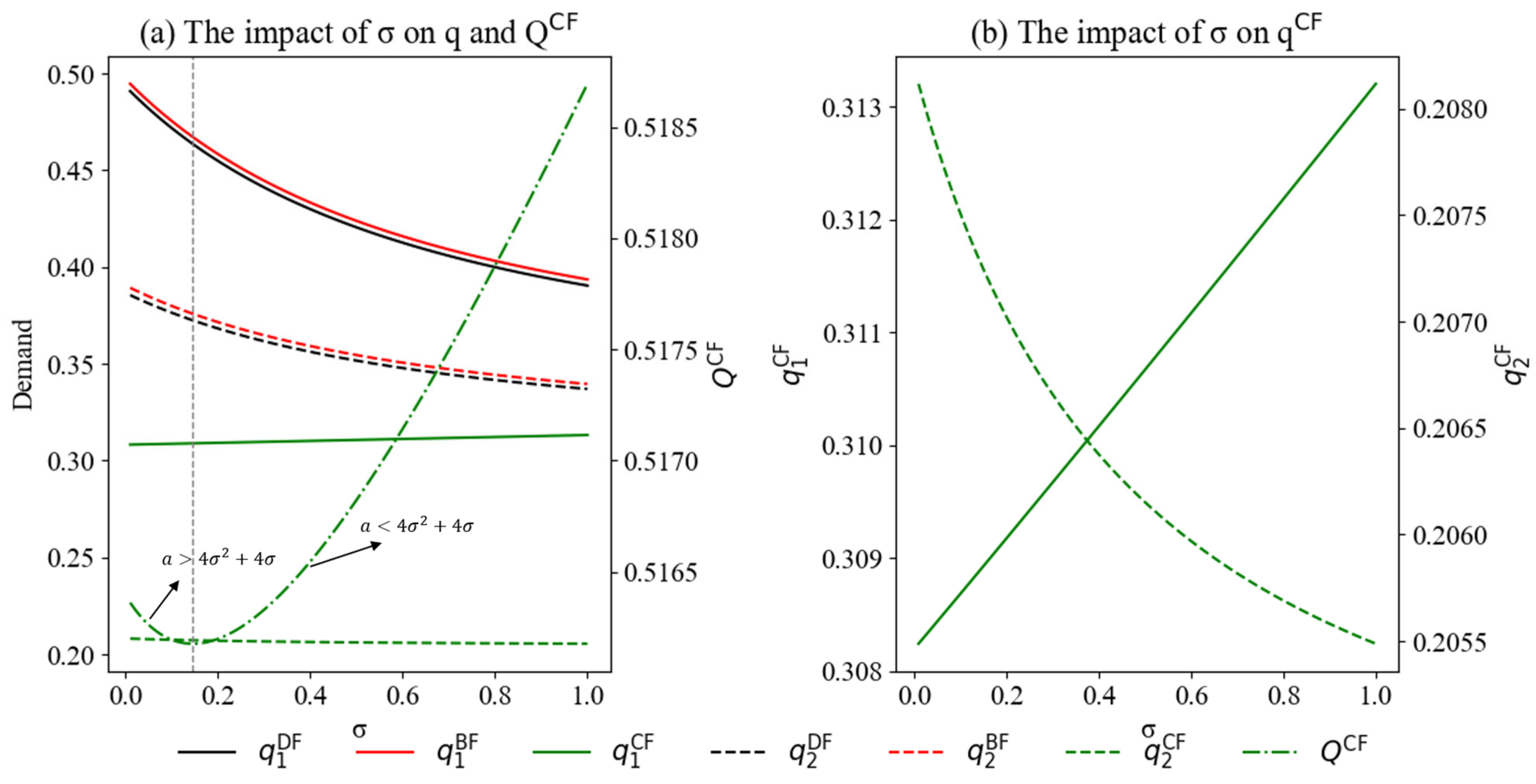
q 1 * C F σ > 0 ; q 2 * C F σ < 0 ; when  a > 4 σ 2 + 4 σ , q 1 * C F σ < q 2 * C F σ , Q * C F σ < 0 ; when  a < 4 σ 2 + 4 σ , q 1 * C F σ > q 2 * C F σ , Q * C F σ > 0 .
(3)
q 1 * B F σ < 0 q 2 * B F σ < 0 q 1 * B F σ > q 2 * B F σ Q * B F σ < 0 .
(4)
q 1 * B F σ > q 1 * D F σ > q 1 * C F σ q 2 * B F σ > q 2 * D F σ > q 2 * C F σ Q * B F σ > Q * D F σ > Q * C F σ .
The proof is detailed in Appendix G.
Proposition 5(1) shows that under Model DF, an increase in ICH reduces the demand for both manufacturers, with a more pronounced decline for the strong manufacturer. GPI efforts lead to higher production costs and, consequently, increased product prices. However, the demand-boosting effect of GPI is insufficient to offset the demand loss resulting from higher prices, leading to an overall decline in market demand. Furthermore, when the strong manufacturer charges a higher price, consumers may shift their purchases to the lower-priced product offered by the weaker manufacturer.
Proposition 5(2) shows that under Model CF, an increase in ICH leads to higher market demand for the strong manufacturer, while demand for the weak counterpart declines. The overall market demand depends on the interplay between the weak manufacturer’s market share and the level of ICH. When the weak manufacturer holds a relatively small market share, the decline in its demand has limited impact on the total market, and the increased demand for the strong manufacturer may dominate, leading to overall demand growth. However, if the weak manufacturer holds a large market share, the negative impact of its demand decline may offset the gains of the strong manufacturer. This weakens the overall effectiveness of GPI in expanding market demand and may hinder its broader diffusion. This dynamic resembles a Gresham-like effect in product markets, where low-innovative offerings crowd out higher-quality green innovations, ultimately discouraging long-term sustainability efforts.
Proposition 5(3) indicates that under Model BF, the effect of ICH on market demand is consistent with that under Model DF. However, Proposition 5(4) shows that this effect is most pronounced in Model BF, where complex interactions and pricing competition intensify the impact of ICH on market positioning and consumer preferences, leading to greater demand fluctuations. In contrast, Model DF exhibits milder effects due to the absence of cooperation, while Model CF, characterized by unified control, suppresses competitive dynamics, limiting the transmission of heterogeneity to market outcomes. Accordingly, manufacturers may adopt appropriate strategies to enhance market demand.
Proposition 6. 
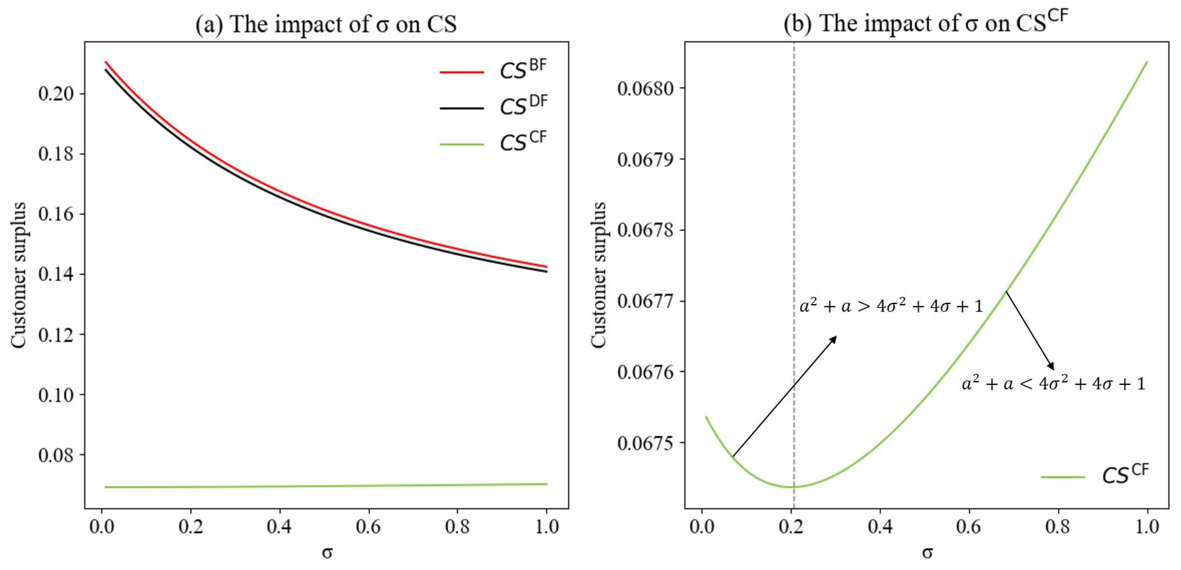
Given that μ is large enough, we have C S * D F σ < 0 ; C S * B F σ < 0 ; C S * C F σ > 0 if a 2 + a < 4 σ 2 + 4 σ + 1 , otherwise C S * C F σ < 0 .
The proof is detailed in Appendix H.
Proposition 6 shows that under the DF and BF Models, increased ICH leads to a decline in CS, primarily due to higher selling prices that narrow the gap between consumers’ willingness to pay and actual prices. Manufacturers should adopt marketing strategies, such as branding and promotions, to raise consumers’ willingness to pay, thereby offsetting the negative impact of higher ICH on CS. Under Model CF, the effect depends on the market size of the weak manufacturer. When the weak manufacturer holds a large market share, increased ICH widens the price gap between manufacturers, allowing the weak manufacturer to attract more consumers and enhance overall CS. In contrast, when the weak manufacturer’s market share is small, rising ICH leads to higher average prices, thereby reducing CS. These results highlight the interaction between ICH, pricing strategies, and market structure.
Proposition 7. 
Given μ is large enough, t i * C F > t i * B F > t i * D F holds.
The proof is detailed in Appendix I.
Proposition 7 shows that GPI investment is highest under Model CF, followed by BF, and lowest under DF. In Model CF, resources across the entire AlBSC are centrally planned and allocated to maximize overall benefit. By reducing unnecessary competition and resource fragmentation, Model CF efficiently integrates capital and technology, thereby maximizing GPI investment. This makes Model CF the ideal framework for fostering GPI. Model BF combines features of both CF and DF. It allows partial central allocation of resources while leaving some decisions to individual participants. As a result, although there is some degree of coordination and resource sharing, residual competition among manufacturers limits integration efficiency compared to Model CF. Thus, GPI investment under BF is lower than in CF but higher than in DF. In Model DF, manufacturers act independently to maximize individual profits. The absence of systemic resource access and coordination leads to cautious investment behavior, especially under market uncertainty. This fragmented decision making results in the lowest level of GPI investment. In light of its potential to improve the efficiency of GPI investment through enhanced coordination and increased resource sharing while retaining operational flexibility, Model BF may represent a preferable option for the AlBSC.
Proposition 8. 
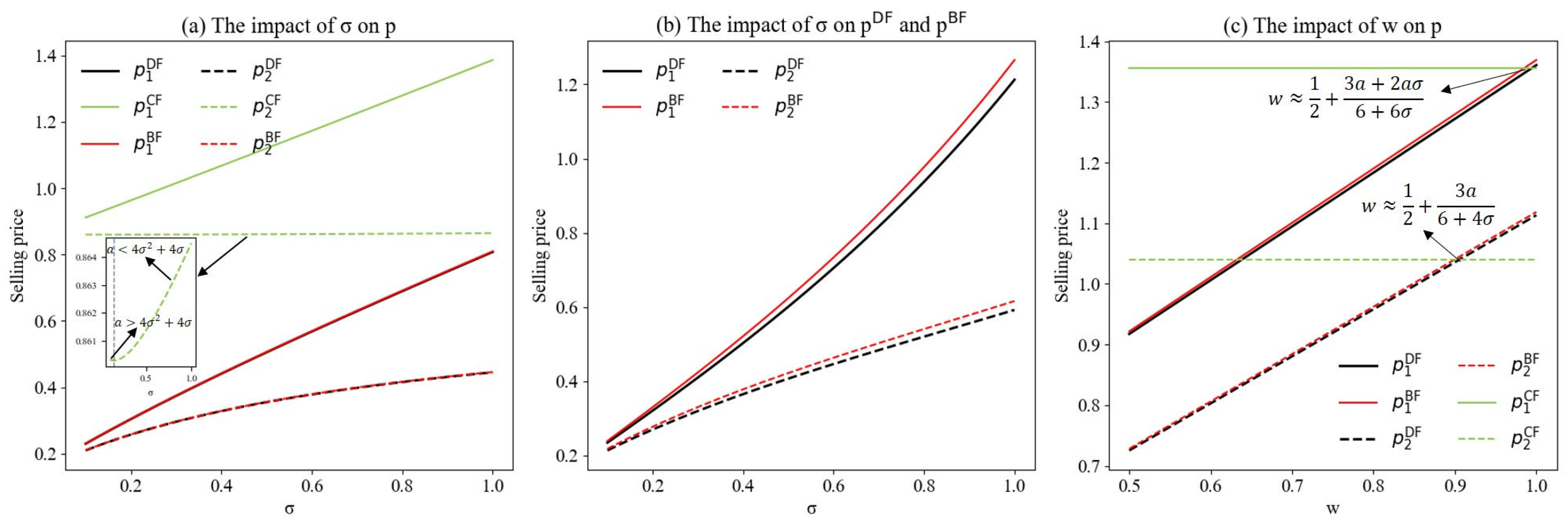
Given μ is large enough, p i * C F > p i * B F > p i * D F when w < 1 2 + 3 a 6 + 4 σ ; p i * B F > p i * D F > p i * C F generally holds when w > 1 2 + 3 a + 2 a σ 6 + 6 σ ; p 1 * B F > p 1 * D F > p 1 * C F and p 2 * C F > p 2 * B F > p 2 * D F when 1 2 + 3 a 6 + 4 σ < w < 1 2 + 3 a + 2 a σ 6 + 6 σ .
The proof is detailed in Appendix J.
Proposition 8 reveals the dynamic nature of selling price ordering across different models as w varies. Specifically, when w is relatively low, Model CF yields the highest selling prices, reflecting the stronger profit integration capability of centralized decision-making. In contrast, when w exceeds the upper threshold, Model BF results in the highest prices, while Model CF yields the lowest, as fully centralized coordination tends to suppress selling prices to mitigate demand loss under high w . Interestingly, within the intermediate range, the price hierarchy diverges between the two manufacturers: for the strong one, Model BF generates the highest price, whereas for the weak one, Model CF prevails. These findings indicate that fluctuations in the wholesale price not only trigger regime shifts in price ordering across decision models but also induce asymmetric pricing effects between competing manufacturers. Therefore, firms should establish flexible contractual and collaborative frameworks to align stakeholder interests effectively in dynamic market environments, thereby enhancing overall supply chain coordination.
Proposition 9. 
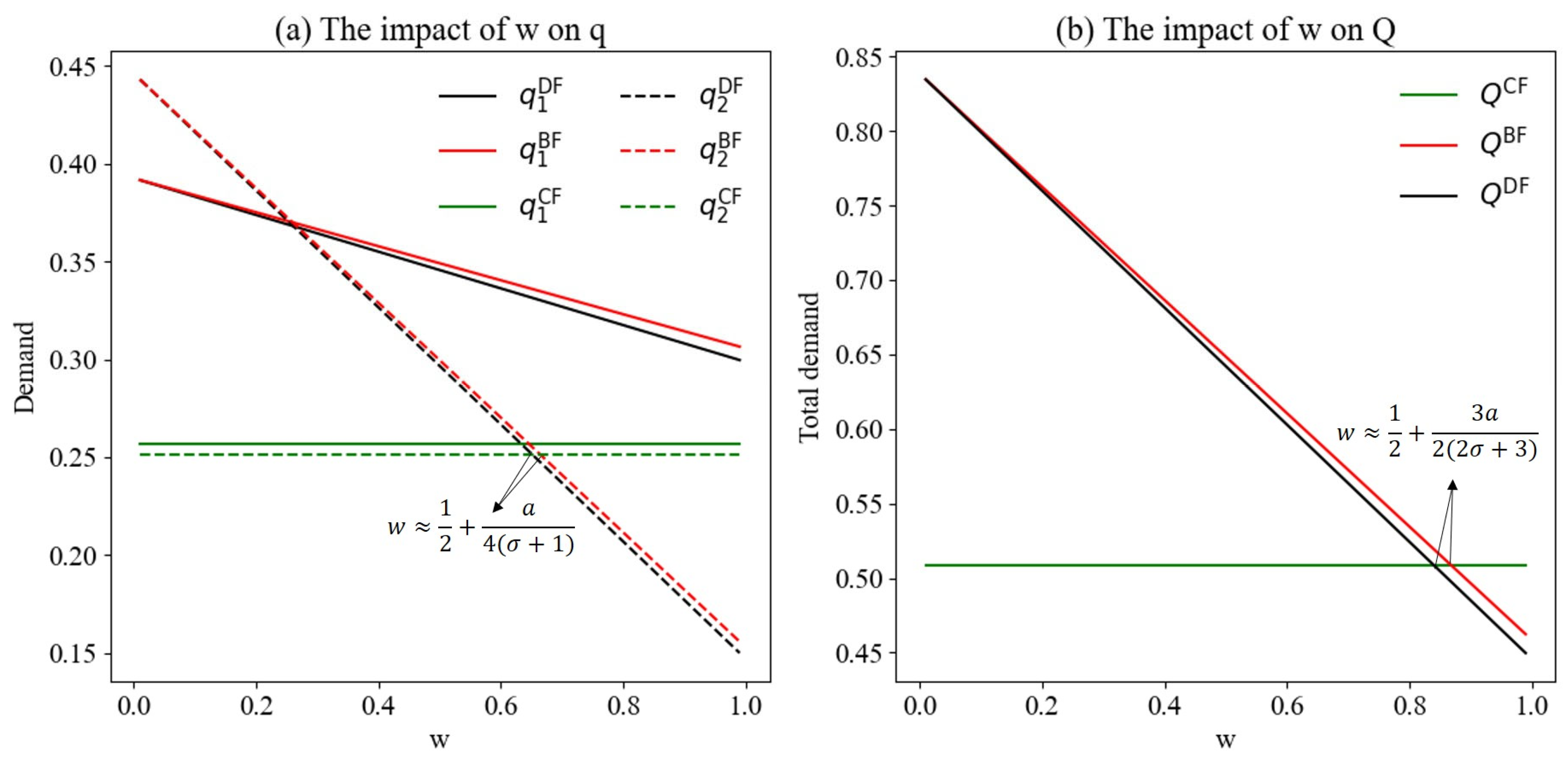
Given μ is large enough, q i * B F > q i * D F > q i * C F when w < 1 2 + a 4 ( σ + 1 ) , otherwise, q 1 * B F > q 1 * D F > q 1 * C F   and q 2 * C F > q 2 * B F > q 2 * D F generally hold. Q * B F > Q * D F > Q * C F if w < 1 2 + 3 a 2 ( 2 σ + 3 ) , otherwise, Q * C F > Q * B F > Q * D F generally holds.
The proof is detailed in Appendix K.
Proposition 9 demonstrates that market demand is generally the highest under Model BF. Although Model DF tends to induce lower prices and thereby higher demand due to intensified competition, Model CF is designed to maximize total supply chain profit, which typically leads to higher prices and reduced demand. These results align with extant literature [29,58]. Notably, Model BF achieves the highest demand in most cases due to its hybrid structure combining cooperation and competition. This arrangement supports greater GPI investment than Model DF and more competitive pricing than Model CF, thereby enhancing perceived value and expanding the consumer base. However, when the wholesale price is sufficiently high, the demand under Model CF surpasses that of BF and DF. In such cases, the centralized coordination in CF helps mitigate demand loss despite higher prices, resulting in relatively greater market demand. Model BF is generally advantageous for expanding market share, and firms should proactively explore and implement this flexible form of cooperation.
Proposition 10. 
Given μ is large enough, if w < 1 2 + a 4 ( σ + 1 ) , C S * B F > C S * D F > C S * C F holds.
The proof is detailed in Appendix L.
Proposition 10 shows that CS is the highest under Model BF when w is not excessively high. Typically, intense competition in decentralized decision making leads to lower selling prices, resulting in higher CS in Model DF compared to Model CF. Model CF entails the highest GPI investment but sets a higher sales price that suppresses demand, resulting in lower CS compared to Model BF. This suggests that price competition between manufactures benefits consumers. However, in Model BF, the combination of cooperation and competition increases market demand and, consequently, CS. The interplay of price competition and innovation cooperation enables consumers to obtain greater value at lower prices than in Model CF, while benefiting from higher market demand, thus further enhancing CS. Hence, it is recommended that the supply chain adopt Model BF, balancing cooperation and competition to enhance market efficiency and customer satisfaction.

5. Extension

As demonstrated above, Model BF achieves a more effective balance across environmental and CS dimensions compared to Model DF. However, given that the supplier actively bears part of the costs associated with downstream GPI, its profitability may be adversely affected [11]. In addition, GPI often incurs high upfront costs and may not generate sharable returns in the short term, rendering revenue-sharing contracts ineffective.
To address this issue, a promotion compensation contract is introduced to offset the supplier’s potential losses. Instead of directly transferring profits to the supplier, the two manufacturers increase their investment in the promotion of green products to stimulate market demand. This demand expansion indirectly enhances the supplier’s profitability, thereby achieving compensation. Let y 1 and y 2 denote the promotion efforts of the two manufacturers, respectively, with a unit promotion cost normalized to 1 for simplicity. Let b denote the demand-boosting effect of promotion. We consider three decision-making scenarios for y 1 and y 2 within a biform game framework: (1) exogenous (Model PBF), (2) endogenous under a cooperative strategy (Model CPBF), and (3) endogenous under a competitive strategy (Model DPBF). In the following, we model each scenario. The profit functions for the three agents are given by Equations (18)–(20).
π S = w 1 + a p 2 1 + a + δ t 1 + δ t 2 + b y 1 + b y 2 μ 2 t 1 2 λ 1 μ 2 1 + σ 1 + σ t 2 2 λ 2
π M f 1 = p 1 w 1 1 + a 1 p 1 p 2 σ + δ t 1 + b y 1 1 2 y 1 2 μ 2 t 1 2 1 λ 1
π M f 2 = p 2 w 1 1 + a a p 2 + p 1 p 2 σ + δ t 2 + b y 2 μ 2 1 + σ 1 + σ t 2 2 1 λ 2 1 2 y 2 2
When y 1 and y 2 are exogenous variables influenced by the external environment or industry conditions, the calculation process, similar to that of Model BF, is omitted for brevity.
When the promotion strategies are treated as endogenous variables, the biform game framework allows y 1 and y 2 to serve as cooperative strategies in the cooperative game part or as competitive strategies in the non-cooperative game part. As the calculation process is similar to Model BF, it is not elaborated further.

6. Numerical Results

To reinforce the empirical validity of the findings, this study conducts further analysis using the aluminum alloy building materials supply chain as a case, comprising one aluminum ingot supplier upstream and two aluminum alloy manufacturers downstream.
Model parameters are set based on publicly available macro-level industry statistics and firm-level data from the aluminum sector. After reasonable simplifications consistent with model assumptions, the simulations capture the behaviors of key supply chain agents and market conditions. Given the difficulty of obtaining complete micro-level data, this approach offers a practical way to demonstrate the model’s applicability and decision-making relevance in real supply chain contexts [59].

6.1. Parameter Setting

The parameters used in the simulation are estimated based on publicly available industry data, patent databases, and relevant literature. To ensure representativeness, aluminum alloy building material is selected as a case study. Although the demand enhancement effect of GPI cannot be directly measured, the growth rate of the Al Alloy sector [60] and related studies [59,61] inform the setting of the demand enhancement coefficient δ   =   0.2 . The wholesale price of aluminum ingots is based on the mode of the London Metal Exchange aluminum closing prices from 1 May 2024, to 1 May 2025, after min–max normalization. The wholesale price is set at 0.15, corresponding to the lower end of the normalized price range and representing a low-price market condition. Additionally, to comprehensively capture wholesale price fluctuations, very low (0.05), medium (0.3), and high (0.6) values are included in the sensitivity analysis to verify the robustness of the model’s conclusions across different market scenarios.
The innovation capability data are sourced from the CSMAR database, which is widely used in finance and industrial research and covers financial, market, and industry-related information of listed companies in China. The data preparation involved the following steps:
Step 1: Sample selection. Given the focus on aluminum building material manufacturers, A-share listed companies in the aluminum rolling and processing industry (Industry Code: C3252) from 2001 to 2021 were selected. A total of 26 companies primarily engaged in the production of architectural aluminum profiles were identified as the sample.
Step 2: Data collection. The number of green patents held by each sample firm was collected to measure their innovation capability.
Step 3: Grouping and calculation. Firms were categorized into high- and low-innovation groups using a threshold of 10 green patents. This grouping does not affect the main findings, as sensitivity analyses on ICH have been conducted to ensure the robustness of results. The ICH was calculated as the ratio of the patent difference between groups to the number in the higher group, with σ = 0.6 and σ   ϵ   [ 0.1 , 1 ] .
According to the market concentration of China’s aluminum processing industry, with a CR10 of 57.46% [62], the market share of the weaker manufacturer is assumed to be 0.4, resulting in the parameter a = 2 / 3 . Based on this baseline, lower (0.25) and higher (0.75) values of a are selected to examine the model’s robustness against market structure variations.
Guided by the Green Manufacturing Project Implementation Guidelines issued by the Ministry of Industry and Information Technology of the People’s Republic of China in 2016, this study sets 2015 as the base year for traditional product innovation (TPI), with its unit innovation cost normalized to 1. The unit cost multiplier for GPI is then measured for 2016 and subsequent years. Drawing on data from A-share listed companies in the aluminum smelting and rolling processing industry that consistently disclosed R&D investment from 2007 to 2024, this study incorporates China’s core inflation rate into the empirical analysis to perform time discounting, thereby controlling for the effect of time. According to data from 2008 to 2025, the average annual core inflation rate is 1.19% [63]. Based on this, it is estimated that the actual unit cost multiplier of GPI relative to TPI falls within the range of [ 1.1 ,   3.7 ] , with an average value of 2.1. This range is also consistent with previous studies [59,61], which set the cost multiplier at 2 or 2.5, serving as a representative value within this interval. Accordingly, we set μ = 2.1 . Sensitivity analysis considers lower (1.5) and higher (3.5) values of μ , representing typical GPI unit costs in the aluminum building materials sector.
Next, we perform sensitivity analyses on the performance of the coordination mechanism, which incorporates the innovative promotion compensation contract, and examine the impact of ICH on the corresponding equilibrium solutions.

6.2. The Impact of ICH on GPI Decisions

The relevant conclusions are obtained by propositional derivation in Section 4. This section is verified by numerical analysis. Figure 3 illustrates the impact of ICH on GPI investment, which corroborates Propositions 3 and 7. As shown in Figure 3a, the difference between t i * B F σ and t i * D F σ is minor. However, compared with Model CF, Model BF significantly enhances how sensitive both manufacturers’ GPI investment is to ICH.
Figure 4 supports Propositions 4 and 8. The empirical results further indicate that the manufacturers’ selling prices under Models BF and DF are nearly identical. However, when δ is relatively high ( δ = 0.9 ), as shown in Figure 4b, Model BF tends to yield slightly higher selling prices than Model DF. Figure 4c further reveals that when the wholesale price is high and within a narrow range, the selling price under Model CF may fall between those of the BF and DF models. This indicates a mild transitional effect near the high-price threshold. Although this does not affect the overall conclusions, it underscores the need for firms to carefully calibrate pricing and cooperation strategies within this sensitive range.
Figure 5 confirms Proposition 5, while Figure 5 supports Proposition 9. As shown in Figure 5a, the demand under Model BF is slightly higher than that under Model DF. Moreover, Figure 6 shows that within certain low wholesale price intervals, demand under Model CF may fall between that of Models BF and DF. Overall, Model BF demonstrates higher demand across most wholesale price ranges, whereas Model CF outperforms the others only under extremely high wholesale prices.
Figure 7 lends support to Propositions 6 and 10. Empirical findings reveal that Model BF results in a marginally higher CS than Model DF, but significantly higher than Model CF.

6.3. The Impact of ICH on Profit Allocation and Profits

Given the complexity of the expressions, we examine the impact of ICH on the cost-sharing ratio and profits through numerical simulations.
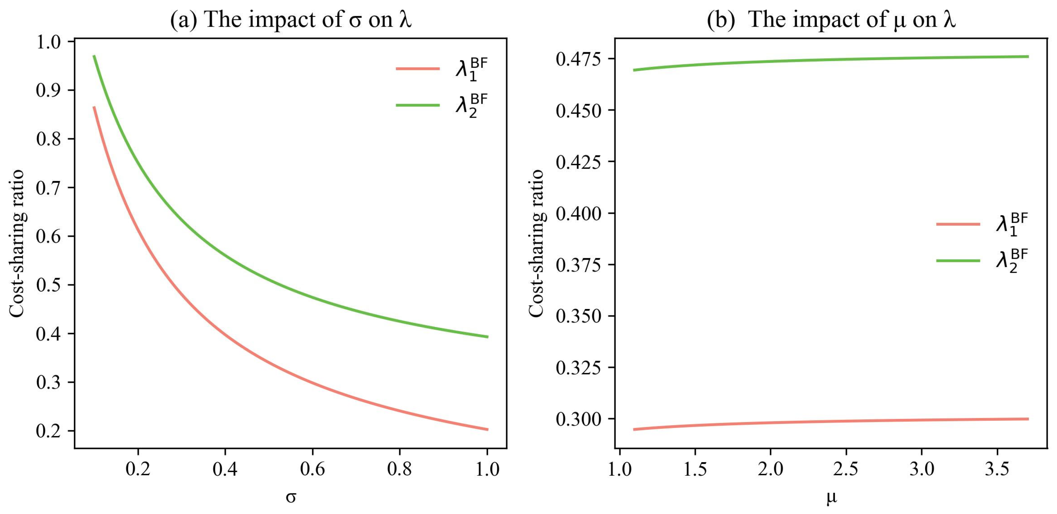
Regarding the cost-sharing ratio, Figure 8 reveals the following key findings: (1) The cost-sharing ratios are positive, indicating that Model BF can incentivize suppliers to share the cost of GPI with manufacturers in the early stages [11]. (2) The supplier shares a higher ratio with the weak manufacturer than with the strong one. This is mainly because the weak manufacturer has limited resource endowments, making the cost of GPI exceed its own capability. (3) Greater ICH leads to lower cost-sharing ratios. For the strong manufacturer, this typically implies less dependence on the supplier. In contrast, the weak manufacturer tends to rely more on supplier support to remain competitive. However, as ICH increases, the supplier may perceive diminishing returns from supporting the weak manufacturer and thus becomes less willing to share the innovation costs. (4) A higher unit cost of innovation leads to an increase in the cost-sharing ratio, but the magnitude of this increase is relatively small. This occurs because the supplier considers the diminishing marginal returns and increased investment risks associated with higher innovation costs, making them less willing to significantly raise the cost-sharing ratio. Therefore, when ICH among downstream manufacturers is high, it is advisable for the supplier to adopt a relatively low cost-sharing ratio. Moreover, as unit innovation costs increase, the supplier should exercise greater prudence in cost-sharing decisions and consider providing technical support to mitigate potential risks.
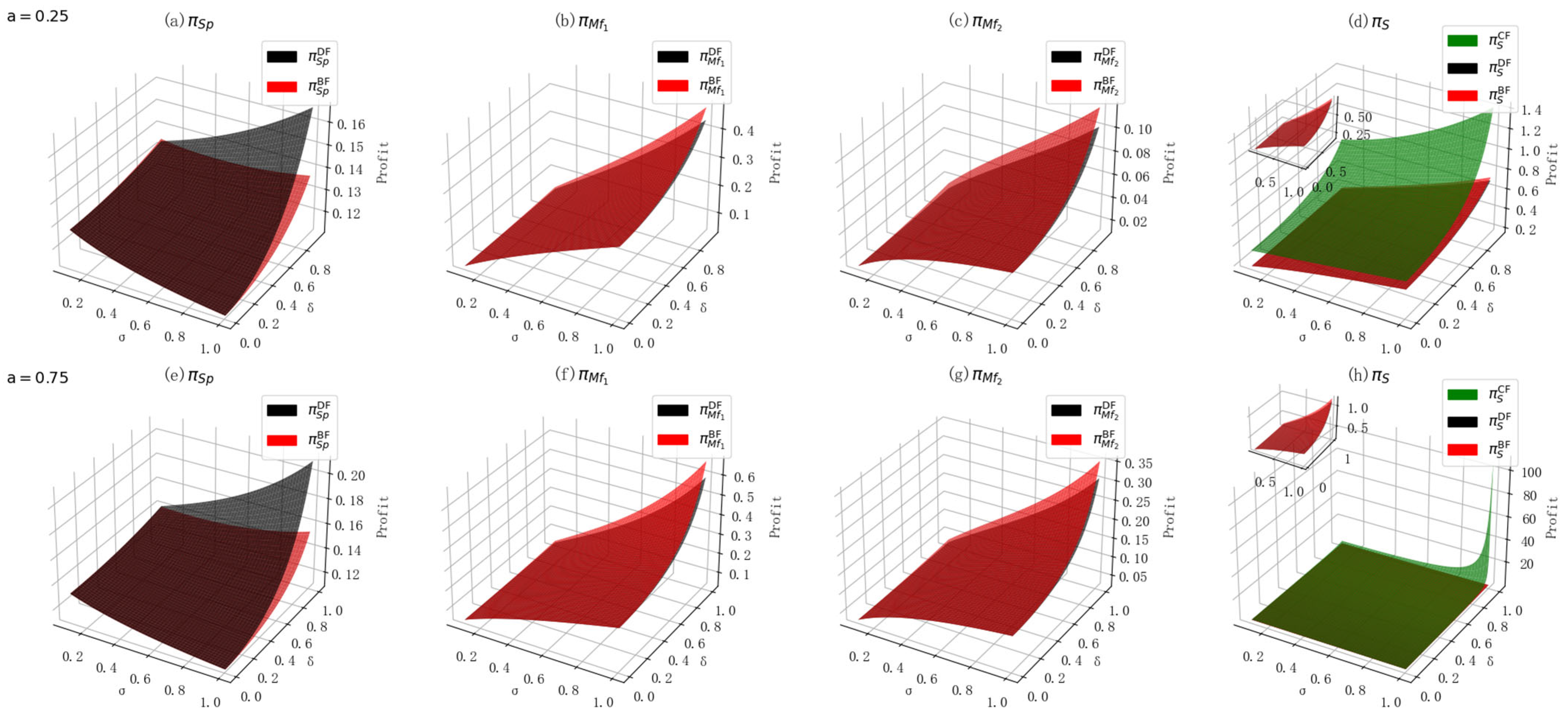
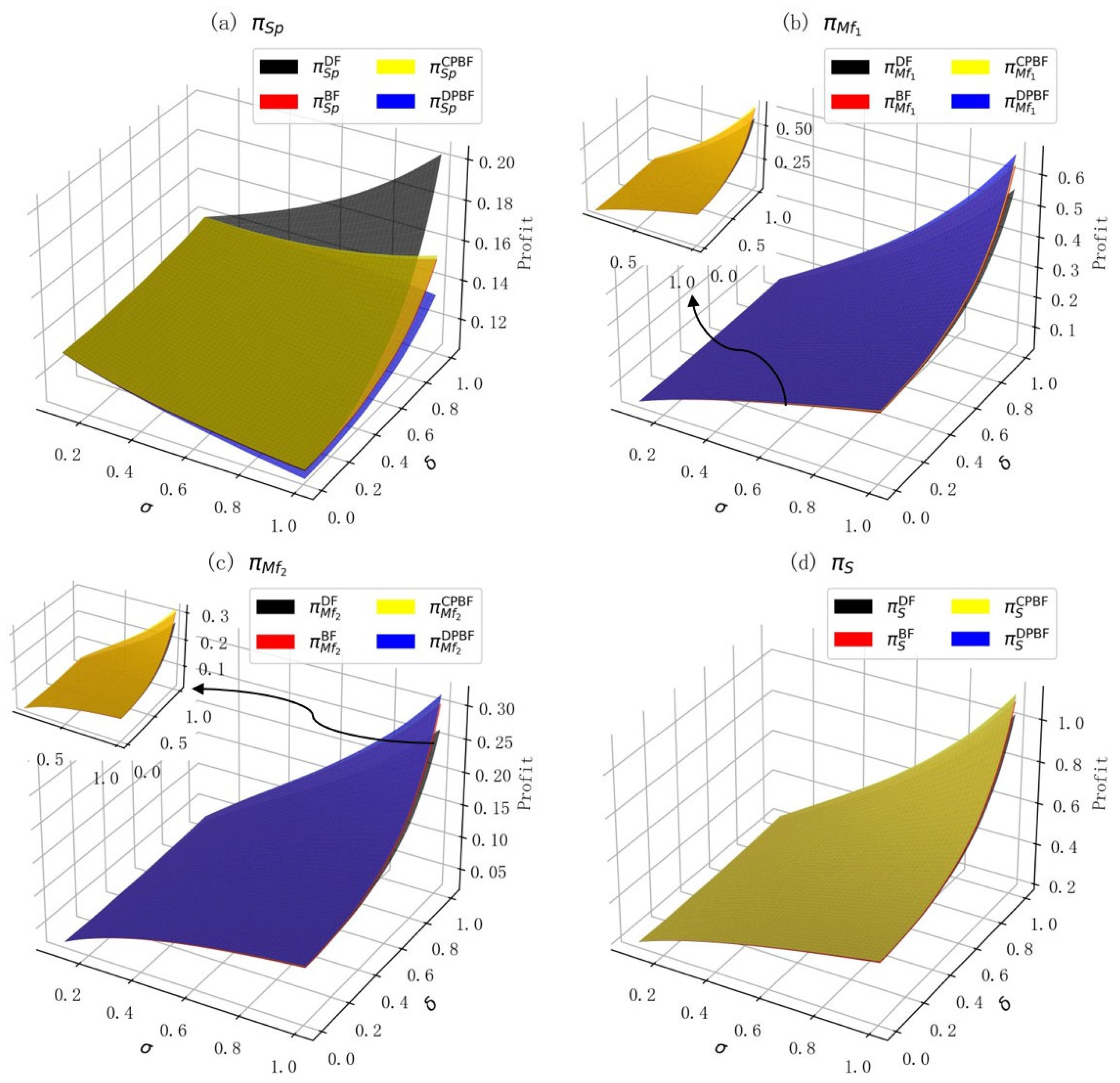
Concerning profits, Figure 9 presents the following key findings: (1) The demand-boosting effect of GPI moderates the impact of ICH on the supplier’s profit, with distinct mechanisms observed under the DF and BF Models. Specifically, when GPI yields limited returns, ICH amplifies competitive imbalance: strong manufacturers are unable to fully capitalize on their capabilities, while the weaker one struggle to remain competitive, leading to weakened realization of green premiums and suppressed supplier profitability. In contrast, when GPI generates substantial market returns, ICH facilitates effective differentiation and market segmentation under Model DF, enhancing channel vitality and enabling the supplier to benefit from a diversified downstream structure. Under Model BF, however, ICH contributes to supplier profit growth only when both ICH and the demand-enhancing effect of GPI are sufficiently high, highlighting the importance of coordinated market strength and innovation capability for realizing upstream profitability.
(2) An increase in ICH leads to increase in the profits of the manufacturers and the supply chain. As the ICH increases, the strong manufacturer can capitalize on its innovation outcomes to strengthen product differentiation, thereby attracting greater market demand. The enhanced competitive advantage enables both manufacturers to command higher retail prices, thereby improving their profitability. However, despite the reduced cost-sharing ratios due to increased heterogeneity, the overall market demand contracts slightly. Since the supplier’s wholesale price remains unchanged, the decline in demand ultimately diminishes the supplier’s profit.
(3) The profits of the two manufacturers and the supply chain are marginally higher in Model BF than in Model DF, indicating that Model BF enhances benefits through cooperation in GPI. This finding aligns with the results of literature [11], further validating the effectiveness of Model BF.
(4) ICH significantly affects the relative advantage of supplier profits under Models BF and DF. When ICH is low, the cooperative nature of Model BF leads to slightly higher supplier profits through more balanced profit sharing. However, when ICH is high, supplier profits under Model DF surpass those in Model BF, as greater ICH creates natural barriers that reduce competition. The competitive strategy in Model DF allows suppliers to capture more profits from differentiation. This indicates that the effectiveness of cooperative versus competitive strategies depends on the degree of ICH, which directly impacts supplier profitability. When incentivizing downstream manufacturers to engage in GPI, suppliers should assess the level of manufacturers’ ICH. Under low ICH, collaboration through Model BF may lead to a more balanced profit distribution. However, when ICH is high, suppliers should carefully evaluate the potential profit constraints imposed by Model BF and consider implementing compensation contracts or adjusting cooperation terms to mitigate possible losses. (5) The profit of the supply chain is maximized under Model CF, which is a well-established result in the existing literature, as it eliminates double marginalization [61].
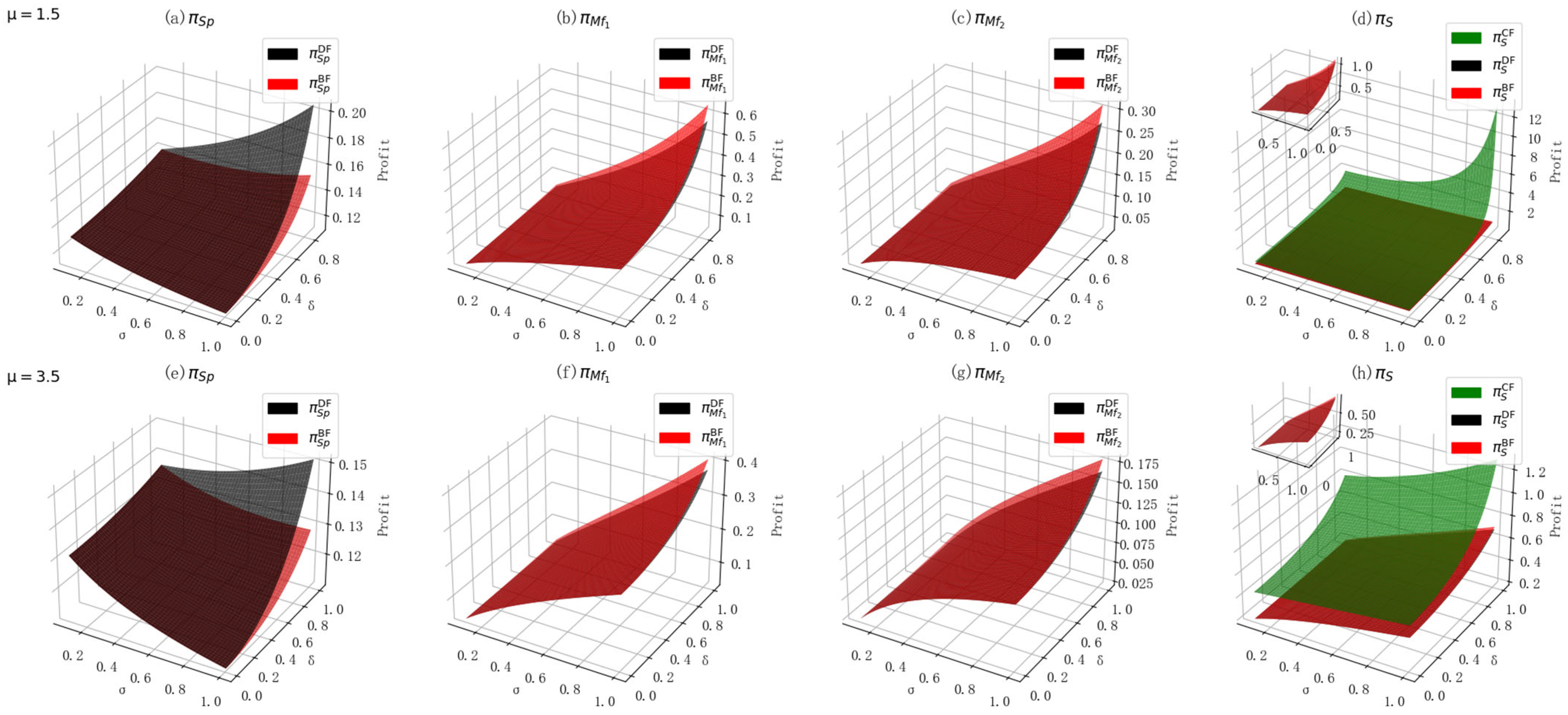
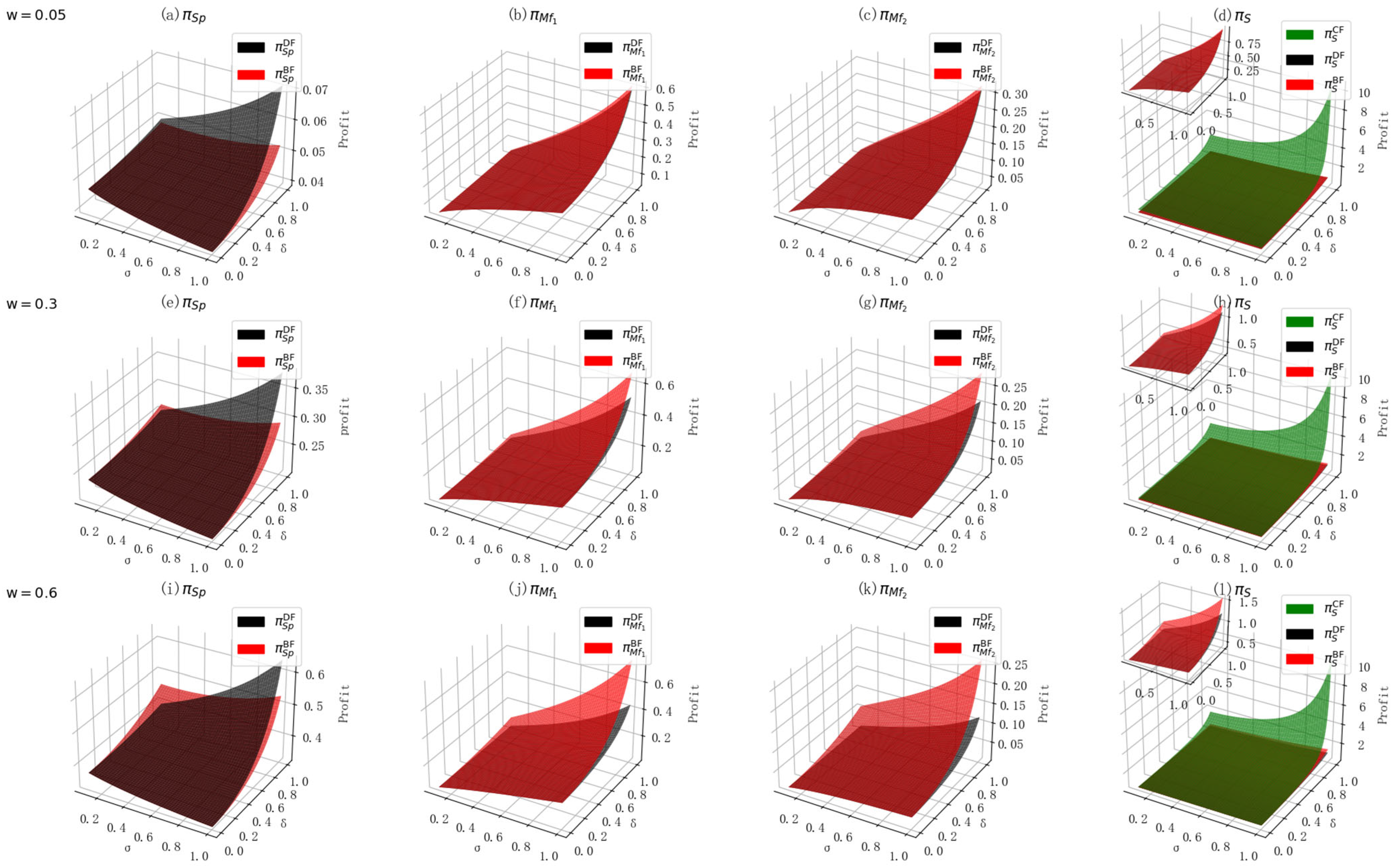
To further validate and enrich the robustness of the findings, sensitivity analyses were conducted on parameters a , w , and μ . The results (see Appendix M) support the main conclusions, while also revealing that when w is relatively high and ICH is low, supplier profits under Model BF exceed those under Model DF. This occurs because higher wholesale prices allocate a greater share of supply chain profits to the supplier. Consequently, even when the supplier bears part of the downstream GPI costs, its own profit is not adversely affected.

6.4. The Impact of ICH on SW

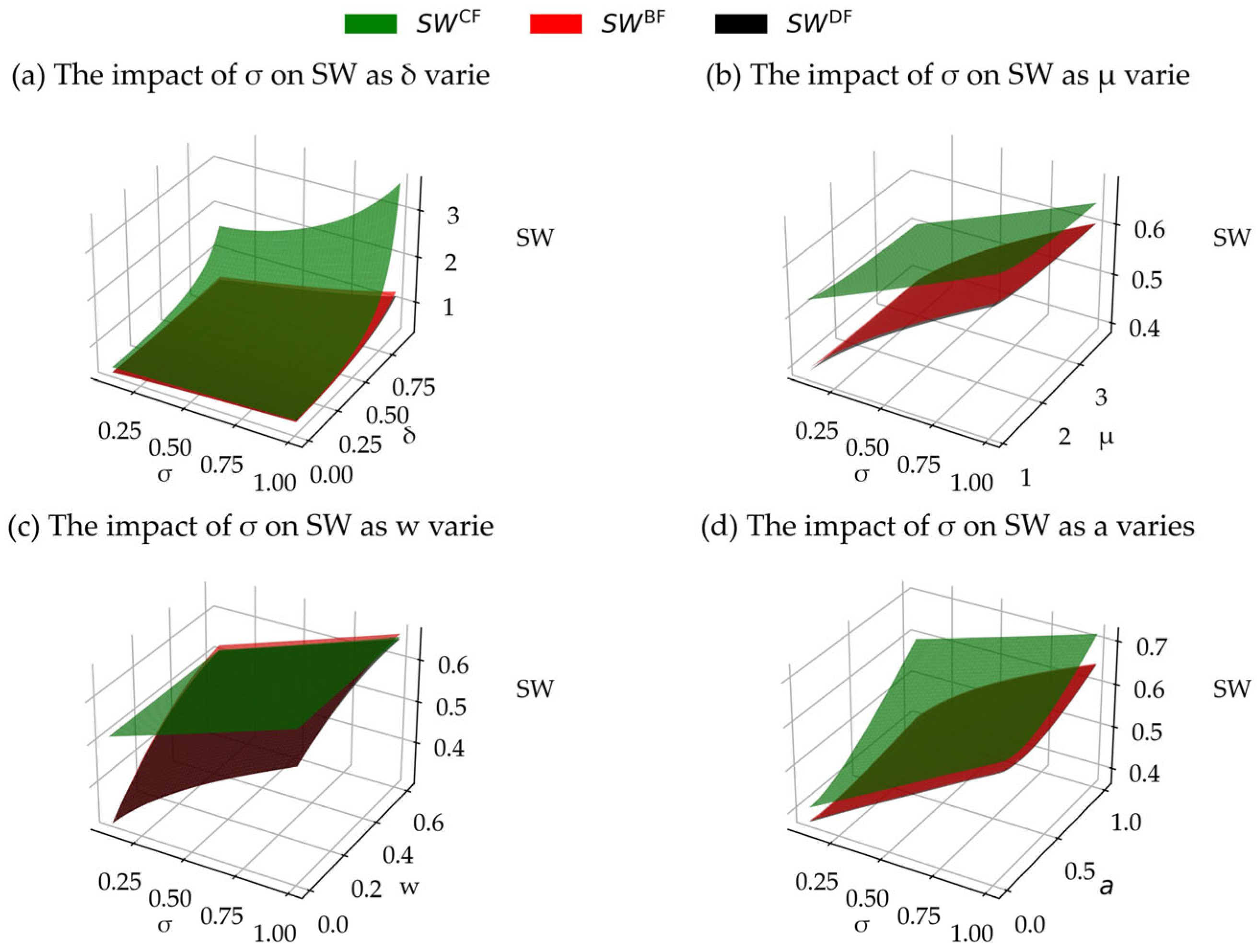
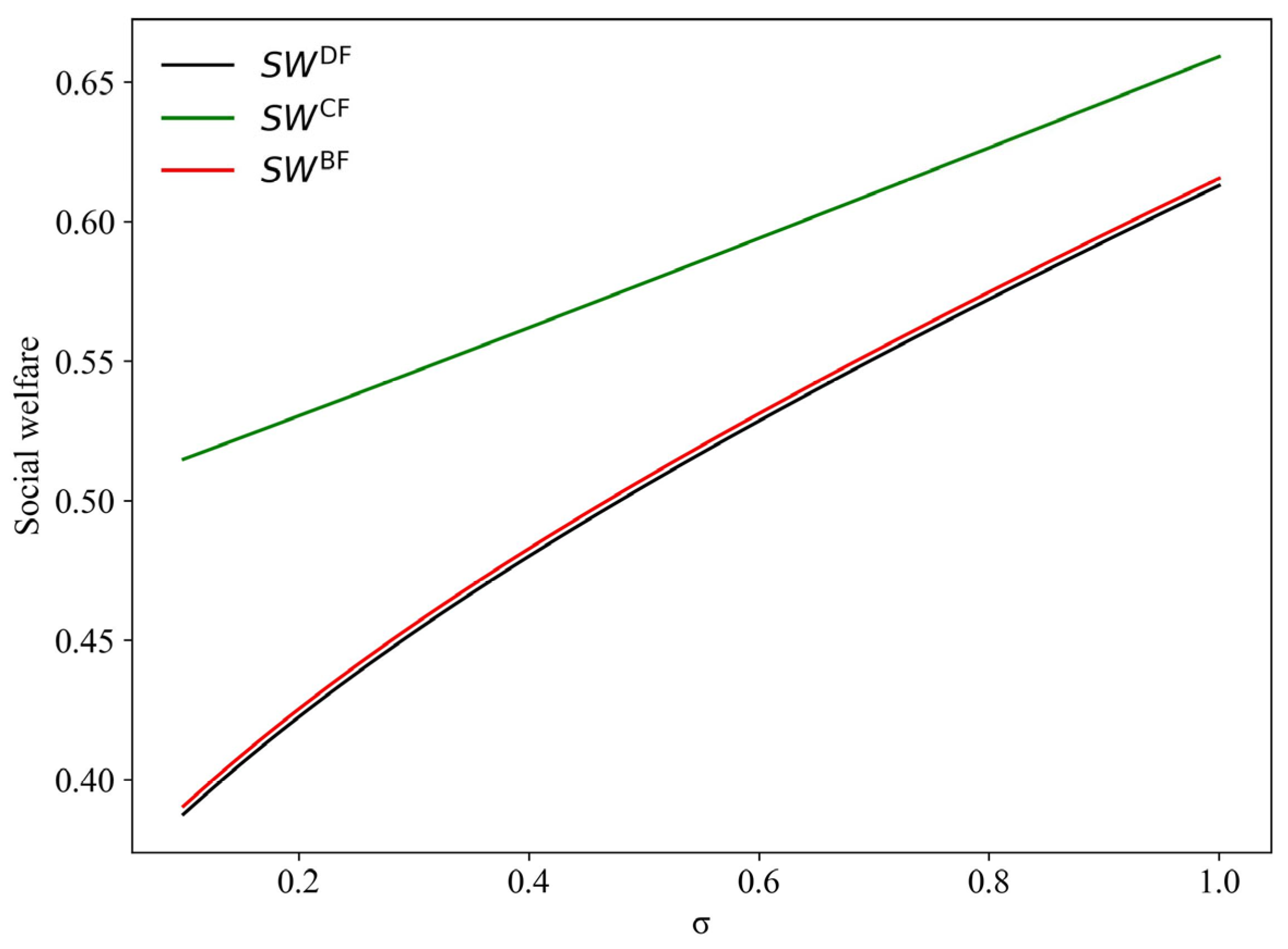
According to ref. [64], social welfare (SW) is defined as S W = π s + C S . As shown in Figure 10, the main conclusions can be drawn and are discussed as follows. (1) The inequality S W * C F > S W * B F > S W * D F indicates that cooperation contributes positively to SW. Model CF primarily enhances overall SW from the perspective of the supply chain, while Model BF better balances CS. For the aluminum industry, this suggests a greater degree of supply chain integration, such as enhanced collaboration between upstream and downstream agents, which can reduce inefficiencies, improve incentive alignment, and ultimately generate higher overall value. (2) With the increase in ICH, SW gradually improves. This suggests that greater heterogeneity promotes a more efficient allocation of resources by directing them toward more innovative and productive entities, which in turn enhances SW. Therefore, the AlBSC incorporates Model BF, thereby enhancing CS and SW. Meanwhile, ICH promotes efficient resource allocation, achieving mutual benefits for both supply chain value and social welfare.
To verify the robustness of the above conclusions, sensitivity analyses were conducted on key parameters δ , a , w , and μ . The results indicate that the conclusions remain consistent, thereby demonstrating robustness (see Appendix M). Only when w is relatively high does SW under Model BF potentially exceed that under Model CF.

6.5. The Coordination Effect of the Promotion Compensation Contract

6.5.1. Exogenous Promotion Compensation

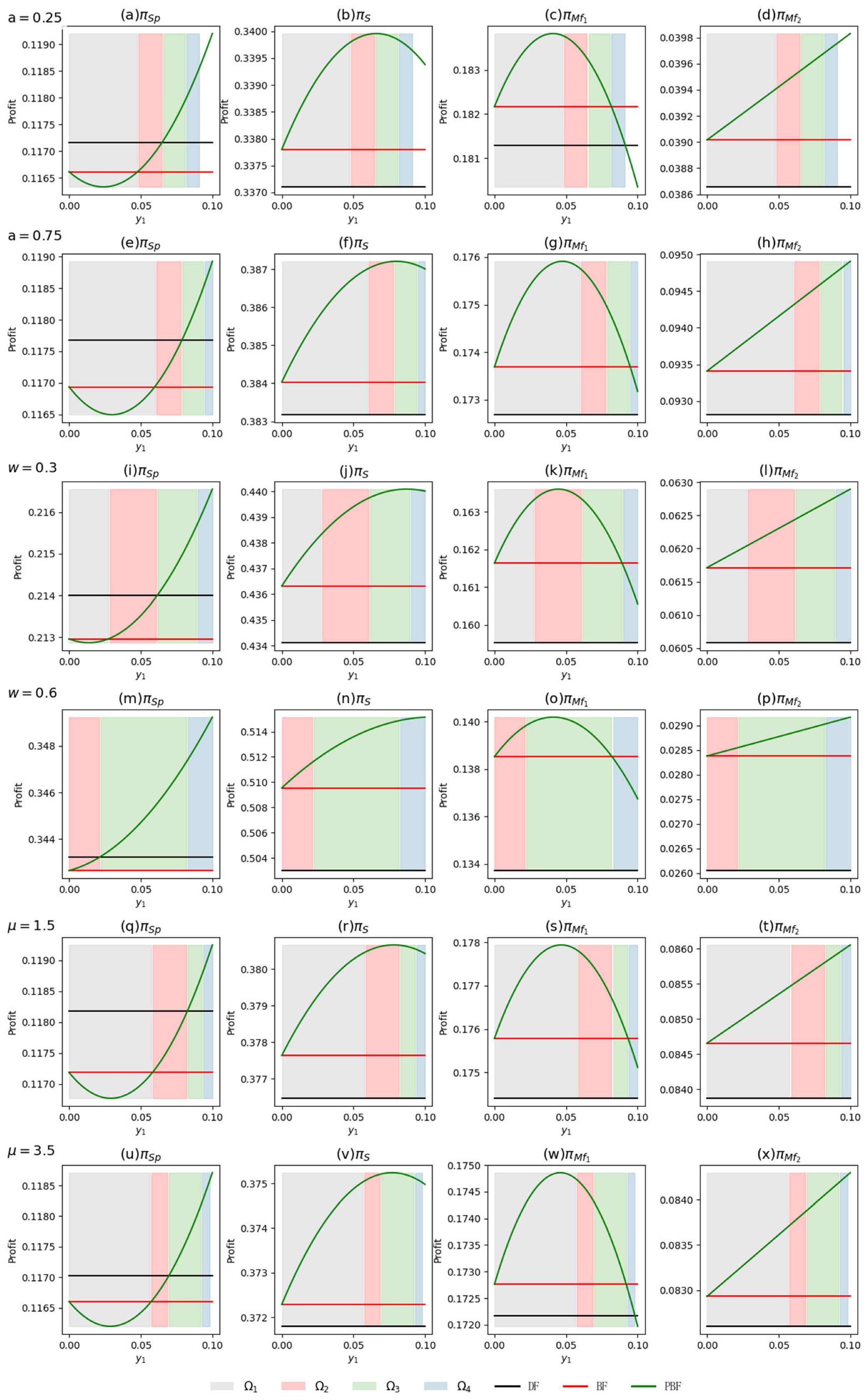
To investigate the effect of the strong manufacturer’s compensation strategy on profits, we set y 2 = 0 . Against the backdrop of a projected 6.21% CAGR for the aluminum alloy industry from 2024 to 2034 [65], it is assumed that promotional investment will lead to a 10% demand enhancement effect. Considering the diminishing marginal returns of promotion efforts, the strong manufacturer, assuming rational behavior, would not increase its promotional investment indefinitely. Based on the analysis of annual reports from the non-ferrous light metal industry for the period 2022–2024, the maximum observed ratio of selling expenses to profits is approximately 11.33%. Given the previously established parameter values, the strong manufacturer’s profit is estimated to be around 0.17. According to the cost function, the maximum value of y 1 is thus inferred to be approximately 0.2. Taking into account that λ i > 0 and the presence of loss aversion among manufacturers, the parameter y 1 is set within the interval ( 0 ,   0.1 ) .
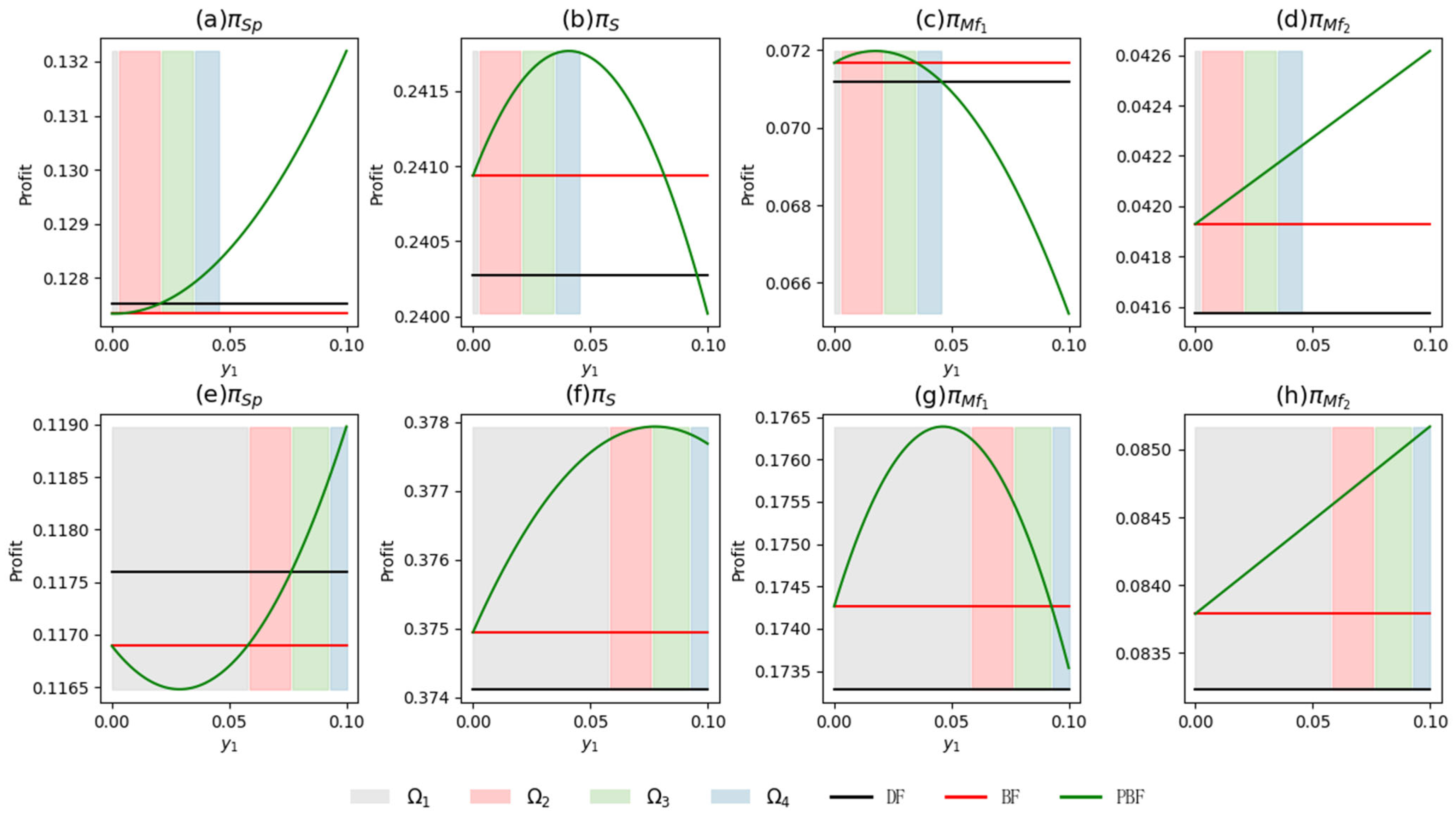
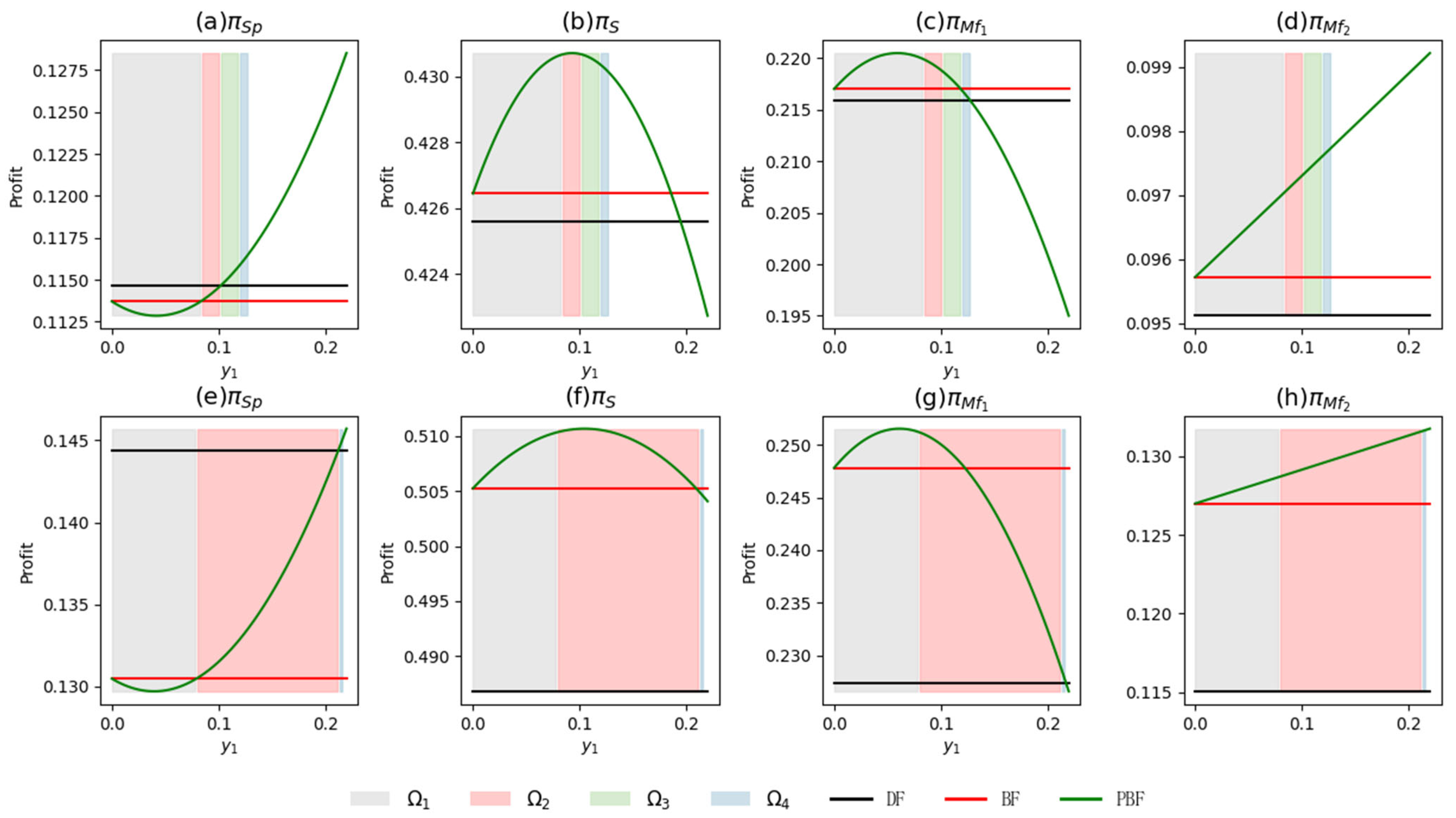
As illustrated in Figure 11, the range of the compensation coefficient can be divided into four distinct zones. Ω 1 : Ineffective zone; the supplier’s profit is lower than that in Models BF and DF. Ω 2 : BF-Dominant Pareto Optimal Zone; both the collective and individual profits exceed those under Model BF. Ω 3 : Strong Pareto Optimal Zone; both the collective and individual profits exceed those under Models BF and DF. Ω 4 : DF-Dominant Pareto Optimal Zone; both the collective and individual profits exceed those under Model DF. Therefore, manufacturers can adopt a low-promotion investment strategy to improve their own profitability as well as that of the supply chain and supplier.
Through a sensitivity analysis of the above conclusions (see Appendix M), the results indicate the following: (1) the core conclusions remain consistent; (2) when ICH and δ are at lower levels, the findings still hold, although the required promotional compensation ratio for achieving Pareto improvements decreases as ICH declines; (3) when ICH is higher, the exogenous mechanism continues to yield Pareto improvements over Model BF, but achieving improvements over both BF and DF requires a higher compensation ratio; and (4) when δ is high, Pareto improvements can only be attained relative to Model BF.
As shown in Figure 12, in all compensation zones, both the level of GPI investment and the SW under Model PBF exceed those under Model BF. While promotion compensation generally enhances investment in GPI, it does not always lead to higher SW. This is because excessively high compensation coefficients can reduce the overall profit of the supply chain, thereby diminishing SW.

6.5.2. Endogenous Promotion Compensation

The following key findings can be drawn from Figure 13: (1) GPI’s demand-enhancing effect significantly moderates the influence of ICH on supplier profitability, aligning with the findings in Section 6.2 and holding under both promotional and non-promotional conditions. (2) Endogenous strategies can yield equilibrium solutions and, under certain conditions, achieve Pareto improvements. Specifically, equilibria exist under both cooperative and competitive strategies; when cooperation is adopted and the demand enhancement effect is relatively weak, the system can realize a Pareto improvement. (3) Cooperative strategies benefit the supplier, while competitive strategies favor the manufacturer. Specifically, the supplier earns slightly more under Model CPBF than Model BF, while Model DPBF results in lower profits than BF. For the manufacturer, endogenous promotional compensation contracts better coordinate the supply chain and increase both manufacturers’ profits, with Model DPBF yielding higher manufacturer profits than Model CPBF. This is attributed to the higher promotional investment under cooperation compared to competition. Firms should adjust contract strategies based on market conditions. Under high market risk, they should prioritize CPBF to share risks and promote collaborative innovation. Conversely, when increased manufacturer profits favor cooperation, firms should adopt DPBF while balancing overall supply chain performance.
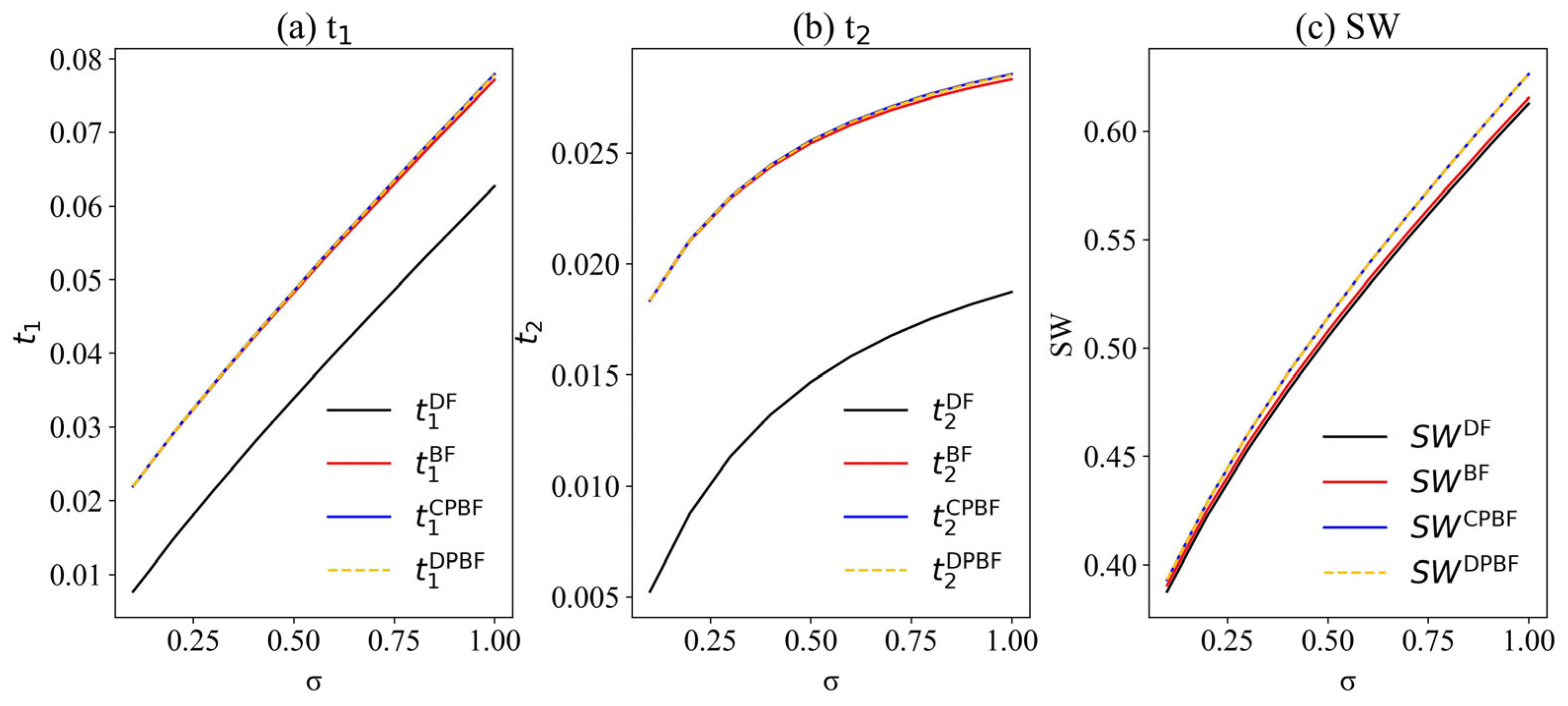
Figure 14 further illustrates the following key finding: decisions based on biform game, with or without promotional compensation mechanisms, are beneficial to the environment and society. Specifically, compared to Models DF and BF, CPBF and DPBF lead to increased GPI investment and higher SW. Moreover, the difference between cooperative and competitive strategies in their impact on GPI and SW is marginal.

6.5.3. Comparison of the Coordination Results Across Different Decision-Making Mode

We further compare the coordination outcomes across the three decision-making modes. Table 4 presents three key findings: (1) The promotion-compensation contracts based on biform game are characterized by multi-perspective coordination, as variations in their design can strategically favor different agents. (2) Exogenous decision making provides higher coordination effectiveness, as it is not influenced by the strategic interactions between agents, whereas endogenous decision making may lead to a weakening or loss of coordination due to game dynamics. This approach bypasses the equilibrium dilemma, achieving system-wide optimal coordination. (3) In endogenous games, cooperation facilitates coordination, while competition exacerbates divergences, particularly disadvantaging the supplier. Supply chain agents should adopt a multi-perspective promotional compensation contract that balances the interests of all parties and facilitates effective coordination. Priority should be given to exogenous decision making mechanisms to avoid coordination failures caused by strategic games.

7. Conclusions

This paper develops an AlBSC model involving a supplier and two manufacturers with ICH investing in GPI. We introduce a novel biform game that jointly optimizes both the GPI investment cooperation strategy and the profit-maximizing strategy to develop a decision-making model, and compare it with the DF and CF Models. Furthermore, we introduce a promotion-compensation contract based on the biform game considering the supplier’s profit loss under Model BF, which incorporates three decision-making modes, enabling multi-perspective coordination paradigm to achieve effective supply chain coordination.
This paper develops an AlBSC model involving a supplier and two manufacturers with ICH, both of whom invest in GPI. A novel biform game is proposed to jointly determine the GPI cooperation strategies and profit-maximizing decisions, and its outcomes are compared with those under DF and CF Models. Furthermore, a promotion-compensation contract is designed based on the biform game to address the supplier’s potential profit loss under Model BF. This framework incorporates three decision-making modes and provides a multi-perspective coordination mechanism to achieve effective AlBSC coordination.

7.1. Key Findings

We summarize the core findings as follows. Table 5 addresses RQ1. As ICH increases, strong manufacturers consistently increase GPI investment. In contrast, weak manufacturers’ GPI investment rises under Model DF but declines under Model CF. In Model BF, GPI investment may either increase or decrease, depending on the interaction among wholesale prices, market size, and ICH. Selling prices rise under both Models DF and BF. Under Model CF, prices for strong manufacturers increase, while those for weak manufacturers may either increase or decrease, depending on the relationship between market size and ICH. Overall, while greater ICH promotes supply chain coordination and delivers economic and social benefits, it complicates the alignment of supplier profits. Nevertheless, higher ICH may cause a decline in supplier profit but does not diminish its willingness to cooperate, as collaboration helps avoid greater losses resulting from inaction.
As for RQ2, Model BF consistently outperforms Model DF across all key indicators, though it does not surpass Model CF. Notably, BF yields higher market demand and CS than CF, suggesting greater market responsiveness and enhanced consumer welfare. As full centralization is often impractical due to organizational and contractual constraints, BF provides a more feasible and effective alternative. By balancing coordination and competitive autonomy, it offers a practical compromise between theoretical optimality and real-world applicability.
While Model BF improves the overall supply chain performance compared to Model DF, it fails to achieve a Pareto improvement, as it leads to supplier losses. This finding is consistent with the results reported by ref. [11]. To address this, we propose a promotion compensation contract based on the biform game framework, which facilitates a multi-perspective coordination paradigm. Specifically, when the compensation coefficient is treated as an exogenous variable, different intervals of its value lead to coordination outcomes that favor either the manufacturer or the supplier, or achieve a globally balanced result. Endogenous cooperative strategies can yield a Pareto improvement, under specific conditions, relative to the outcomes of Models BF and DF. Notably, endogenous compensation reveals the principle of ‘cooperation to benefit the supplier, competition to benefit the manufacturer.’ In uncertain environments, this contract offers a more flexible and resilient mechanism, enhancing adaptability to market fluctuations and policy changes.

7.2. Managerial Implications

Our results unveil the following managerial insights, which are synthesized and visually presented in Figure 15. Based on this summary, the key managerial implications are as follows.
(1) Suppliers are advised to adopt differentiated cooperation strategies based on downstream manufacturers’ innovation capabilities and market-driving power. Rather than passively relying on manufacturers’ GPI efforts or exclusively favoring dominant partners, suppliers should proactively identify those able to convert innovation into market performance. Investment in green collaboration is justified only when both technological and commercial potential are evident. Moreover, the supplier can motivate downstream manufacturers by designing a win–win promotional compensation contract. When contract parameters are exogenous, the supplier should aim to secure the highest possible compensation within a reasonable range; when parameters are endogenous, choosing a cooperative decision will lead to more favorable outcomes for the themselves. In practice, tools such as customer analytics, innovation records, and third-party green certifications can assist in partner evaluation. For the AlBSC, adopting Model BF is recommended, as it generally leads to more optimal environmental, economic, and social outcomes compared to Model DF.
(2) For manufacturers, forming partnerships is the optimal decision, as appropriate collaboration supports their green transition. While compensating suppliers may result in some profit loss, as long as compensation is not excessive, the manufacturer’s profit will always exceed that of non-cooperation. Regarding supply chain coordination mechanisms, it is recommended that AlBSC adopt a multi-perspective promotion compensation contract based on biform game. To effectively implement the promotional compensation contract, manufacturers may utilize diversified marketing channels, such as participating in large-scale trade fairs and industry exhibitions. Promotion investment strategies should be based on actual conditions. Specifically, firms can flexibly adjust incentive structures and cost-sharing ratios in response to external changes, thereby maintaining the effectiveness of both coordination and incentives. Moreover, when certain environmental factors (e.g., unfavorable policies or intensified market competition) disadvantage one party, the contract can be adapted to favor the disadvantaged party through multi-promotion compensation strategies to maintain stable cooperation. This flexibility helps stabilize cooperation and fosters more resilient, sustainable supply chain collaborations.
(3) In addition, this study offers valuable insights for policymaking. Given manufacturers’ ICH, policymakers should adopt differentiated strategies tailored to firms’ innovation capacity and market transformation potential. For manufacturers with strong innovation capabilities and commercialization prospects, targeted incentives such as R&D subsidies, tax relief, or technical support can accelerate the adoption and diffusion of GPI. For suppliers whose profits may be adversely affected by participating in GPI collaboration, supportive policies should facilitate fairness. Furthermore, policy interventions should be dynamically adjusted based on demand-side conditions. When green product demand is strong, supply-side support (e.g., innovation grants or production incentives) should be prioritized. Conversely, under weak demand, greater emphasis should be placed on consumer-side measures such as subsidies, public awareness campaigns, or green public procurement to stimulate market development and prevent resource misallocation.
(4) Although this study assumes a relatively stable policy environment, in reality, carbon tax policies, green subsidies, and environmental regulations often experience significant fluctuations and uncertainties. Sudden policy changes may substantially affect firms’ GPI investment and pricing strategies. Specifically, when environmental policies become more stringent, such as through increased carbon taxes, supply chain agents face greater external pressures. Models CF and BF can more effectively foster upstream–downstream collaboration, enabling firms to share policy-related risks, enhance GPI investment, and improve overall supply chain performance. Conversely, when environmental policies are relaxed, external pressure for GPI weakens. Nevertheless, under Model BF, the AlBSC can still maintain a certain level of collaboration, strengthening green resilience and its capacity for continuous improvement.

7.3. Limitations and Possible Directions

This study is not exempt from limitations. It is based on a simplified supply chain structure, which facilitates broad applicability of the results. However, real-world supply chains are often more complex, involving multiple tiers and diverse actors. Future research could extend the model to multi-tier supply chains to improve the generalizability of the findings. Moreover, bounded rationality and information asymmetry, which commonly occur in practice, may affect GPI coordination and could be incorporated into future models. Finally, this paper analyzes scenarios under known market demand conditions, while future studies could consider uncertainty in supply and demand by incorporating stochastic variables.

Author Contributions

Data curation, M.W.; Formal analysis, M.W.; Investigation, M.W.; Methodology, M.W.; Supervision, R.K. and J.L.; Writing—original draft, M.W.; Writing—review and editing, M.W. and J.L. All authors have read and agreed to the published version of the manuscript.

Funding

This research received no external funding.

Data Availability Statement

Data and material will be made available on request.

Acknowledgments

The authors appreciate the valuable comments of the editors and reviewers.

Conflicts of Interest

The authors declare no conflicts of interest.

Appendix A

To derive the equilibrium pricing and green product innovation levels of the two manufacturers under Model DF, the Hessian matrices of their profit functions, π m f 1 and π m f 2 , are first calculated, resulting in H m f 1 and H m f 2 , as shown in Equations (A1) and (A2).
H m f 1 = 2 a σ + σ δ δ μ
H m f 2 = 2 2 σ a σ + σ δ δ μ 2 σ + 1 σ + 1
The Hessian matrices have negative leading principal minors of the first order and positive ones of the second order, indicating that the matrices are negative definite and that a maximum exists. Based on the profit functions of the two manufacturers, the first-order derivatives of π M f 1 with respect to p 1 and t 1 , and of π m f 2 with respect to p 2 and t 2 , are taken and set to zero, yielding the following:
π m f 1 p 1 = a t 1 δ σ 2 p 1 + p 2 + t 1 δ σ + w + σ a σ + σ = 0 π m f 1 t 1 = p 1 δ t 1 μ w δ = 0 π m f 2 p 2 = a t 2 δ σ + a σ + p 1 2 p 2 σ 2 p 2 + t 2 δ σ + w σ + w a σ + σ = 0 π m f 2 t 2 = p 2 δ σ + p 2 δ 2 t 2 μ σ t 2 μ w δ σ w δ σ + 1 = 0
The equilibrium solution of Model DF is derived by solving Equation (A3), as presented in Equations (A4)–(A7). The profits of each agent can be obtained by bringing Equations (A4)–(A7) into Equations (3)–(5).
p 1 * N F = ( a 2 w δ 4 σ 3 + a 2 w δ 4 σ 2 + 2 a w δ 4 σ 3 + 2 a w δ 4 σ 2 4 a w δ 2 μ σ 3 8 a w δ 2 μ σ 2 4 a w δ 2 μ σ a δ 2 μ σ 3 a δ 2 μ σ 2 + 2 a μ 2 σ 2 + a μ 2 σ + w δ 4 σ 3 + w δ 4 σ 2 4 w δ 2 μ σ 3 8 w δ 2 μ σ 2 4 w δ 2 μ σ + 6 w μ 2 σ 2 + 3 w μ 2 δ 2 μ σ 3 δ 2 μ σ 2 + 9 w μ 2 σ + 4 μ 2 σ 3 + 6 μ 2 σ 2 + 2 μ 2 σ ) / a 2 δ 4 σ 3 + a 2 δ 4 σ 2 + 2 a δ 4 σ 3 + 2 a δ 4 σ 2 4 a δ 2 μ σ 3 8 a δ 2 μ σ 2 4 a δ 2 μ σ + δ 4 σ 3 + δ 4 σ 2 4 δ 2 μ σ 3 8 δ 2 μ σ 2 4 δ 2 μ σ + 8 μ 2 σ 2 + 10 μ 2 σ + 3 μ 2
p 2 * N F = ( a 2 w δ 4 σ 3 + a 2 w δ 4 σ 2 2 a 2 δ 2 μ σ 3 a 2 δ 2 μ σ 2 + 2 a w δ 4 σ 3 + 2 a w δ 4 σ 2 2 a w δ 2 μ σ 3 7 a w δ 2 μ σ 2 4 a w δ 2 μ σ 2 a δ 2 μ σ 3 2 w δ 2 μ σ 3 7 w δ 2 μ σ 2 a δ 2 μ σ 2 + 2 a μ 2 σ + w δ 4 σ 3 + w δ 4 σ 2 4 w δ 2 μ σ + 4 w μ 2 σ 2 + 8 w μ 2 σ + 4 a μ 2 σ 2 + 3 w μ 2 + 2 μ 2 σ 2 + μ 2 σ ) / ( a 2 δ 4 σ 3 + a 2 δ 4 σ 2 + 2 a δ 4 σ 3 + 2 a δ 4 σ 2 4 a δ 2 μ σ 3 8 a δ 2 μ σ 2 4 a δ 2 μ σ + δ 4 σ 3 + δ 4 σ 2 4 δ 2 μ σ 3 8 δ 2 μ σ 2 4 δ 2 μ σ + 8 μ 2 σ 2 + 10 μ 2 σ + 3 μ 2 )
t 1 * N F = 2 a δ μ σ 2 a δ 3 σ 3 a δ 3 σ 2 + a δ μ σ 2 w δ μ σ 2 w δ μ σ δ 3 σ 3 δ 3 σ 2 + 4 δ μ σ 3 + 6 δ μ σ 2 + 2 δ μ σ / ( a 2 δ 4 σ 3 + a 2 δ 4 σ 2 + 2 a δ 4 σ 3 + 2 a δ 4 σ 2 4 a δ 2 μ σ 3 8 a δ 2 μ σ 2 4 a δ 2 μ σ + δ 4 σ 3 + δ 4 σ 2 4 δ 2 μ σ 3 8 δ 2 μ σ 2 4 δ 2 μ σ + 8 μ 2 σ 2 + 10 μ 2 σ + 3 μ 2 )
t 2 * N F = a w δ 3 σ 3 + a w δ 3 σ 2 a 2 δ 3 σ 3 a 2 δ 3 σ 2 a δ 3 σ 3 a δ 3 σ 2 + 2 a δ μ σ + w δ 3 σ 3 + w δ 3 σ 2 2 w δ μ σ 2 2 w δ μ σ + δ μ σ 2 + δ μ σ / ( a 2 δ 4 σ 3 + a 2 δ 4 σ 2 + 2 a δ 4 σ 3 + 2 a δ 4 σ 2 4 a δ 2 μ σ 3 8 a δ 2 μ σ 2 4 a δ 2 μ σ + δ 4 σ 3 + δ 4 σ 2 4 δ 2 μ σ 3 8 δ 2 μ σ 2 4 δ 2 μ σ + 8 μ 2 σ 2 + 10 μ 2 σ + 3 μ 2 )

Appendix B

To derive the equilibrium pricing and green product innovation levels under Model CF, the profit function of the supply chain is first formulated, as shown in Equation (A8).
π s = p 1 1 1 + a 1 p 1 p 2 σ + δ t 1 + p 2 1 1 + a a p 2 + p 1 p 2 σ + δ t 2 μ 2 t 1 2 μ 2 1 + σ 1 + σ t 2 2
To ensure the existence of an equilibrium solution, the Hessian matrix of π s is first derived, as shown in Equation (A9).
H s = 2 a + 1 σ δ 2 a + 1 σ 0 δ μ 0 0 2 a + 1 σ 0 2 1 + σ a + 1 σ δ 0 0 δ μ 2 + σ 1 + σ
The diagonal elements of H s are negative, implying that all eigenvalues are negative. Therefore, the Hessian matrix is negative definite, and the function has a maximum.
Based on Equation (A8), the first-order derivatives of π S C F with respect to p 1 , t 1 , p 2 , and t 2 are taken and set to zero, yielding the following:
π s p 1 = a t 1 δ σ 2 p 1 + p 2 + t 1 δ σ + w + σ a σ + σ = 0 π s t 1 = p 1 δ t 1 μ w δ = 0 π s p 2 = a t 2 δ σ + a σ + p 1 2 p 2 σ 2 p 2 + t 2 δ σ + w σ + w a σ + σ = 0 π s t 2 = p 2 δ σ + p 2 δ 2 t 2 μ σ t 2 μ w δ σ w δ σ + 1 = 0
By solving Equation (A10), the equilibrium solution under Model CF is obtained, as shown in Equations (A11)–(A14). The total profit of the supply chain can be obtained by bringing Equations (A11)–(A14) into Equation (A8).
p 1 * C F = μ 4 a μ σ + 2 a μ a δ 2 σ 2 a δ 2 σ δ 2 σ 2 δ 2 σ + 4 μ σ 2 + 6 μ σ + 2 μ / a 2 δ 4 σ 2 + a 2 δ 4 σ + 2 a δ 4 σ 2 + 2 a δ 4 σ 4 a δ 2 μ σ 2 8 a δ 2 μ σ + δ 4 σ 2 4 a δ 2 μ + δ 4 σ 4 δ 2 μ σ 2 8 δ 2 μ σ 4 δ 2 μ + 8 μ 2 σ + 4 μ 2
p 2 * C F = μ a + 1 2 σ + 1 2 μ a δ 2 σ / a 2 δ 4 σ 2 + a 2 δ 4 σ + 2 a δ 4 σ 2 + 2 a δ 4 σ 4 a δ 2 μ σ 2 8 a δ 2 μ σ 4 a δ 2 μ + δ 4 σ 2 + δ 4 σ 4 δ 2 μ σ 2 8 δ 2 μ σ 4 δ 2 μ + 8 μ 2 σ + 4 μ 2
t 1 * C F = δ 4 a μ σ + 2 a μ a δ 2 σ 2 a δ 2 σ δ 2 σ 2 δ 2 σ + 4 μ σ 2 + 6 μ σ + 2 μ / a 2 δ 4 σ 2 + a 2 δ 4 σ + 2 a δ 4 σ 2 + 2 a δ 4 σ 4 a δ 2 μ σ 2 8 a δ 2 μ σ 4 a δ 2 μ + δ 4 σ 2 + δ 4 σ 4 δ 2 μ σ 2 8 δ 2 μ σ 4 δ 2 μ + 8 μ 2 σ + 4 μ 2
t 2 * C F = δ a + 1 σ + 1 2 μ a δ 2 σ / a 2 δ 4 σ 2 + a 2 δ 4 σ + 2 a δ 4 σ 2 + 2 a δ 4 σ 4 a δ 2 μ σ 2 8 a δ 2 μ σ 4 a δ 2 μ + δ 4 σ 2 + δ 4 σ 4 δ 2 μ σ 2 8 δ 2 μ σ 4 δ 2 μ + 8 μ 2 σ + 4 μ 2

Appendix C

Drawing on the profit functions of the supplier and the two manufacturers, the characteristic values of all possible coalitions are derived.
(1)
V p 1 , p 2 ϕ = 0 .
(2)
V p 1 , p 2 S
S acts as a single-player coalition, with the alliance { M f 1 , M f 2 } acting as its opponent. The maximum profit of S acting alone needs to be determined. Assuming the competitive environment in the non-cooperative game is given by ( p 1 ,   p 2 ) , the value function V p 1 ,   p 2   S   depends on the strategy ( λ 1 , λ 2 ) of S , and the strategy t 1 , t 2 of the alliance { M f 1 , M f 2 } . By applying the max-min principle, the following expression is obtained as Equation (A15).
V p 1 , p 2   S   = max λ 1 , λ 2   min t 1 , t 2 { w 1 + a p 2 1 + a + δ t 1 + δ t 2 μ 2 t 1 2 λ 1       μ 2 1 + σ 1 + σ t 2 2 λ 2 } = min t 1 , t 2   max λ 1 , λ 2 { w 1 + a p 2 1 + a + δ t 1 + δ t 2 μ 2 t 1 2 λ 1 μ 2 1 + σ 1 + σ t 2 2 λ 2 }
Since the coefficients of λ 1 and λ 2 are both non-positive, the internal function reaches its maximum value when both are equal to zero. In this case, V p 1 ,   p 2   S   = min t 1 , t 2 { w 1 + a p 2 1 + a + δ t 1 + δ t 2 } . Given that the coefficients of t 1 and t 2 are non-negative, the function value is minimized when both are zero. Consequently, the characteristic value for the supplier acting alone is V p 1 ,   p 2   S   = w ( 1 + a p 2 1 + a ).
(3)
V p 1 ,   p 2   M f 1
When M f 1 forms a singleton coalition, the alliance { S , M f 2 } acts as its opponent. The maximum profit of M f 1 acting alone is given by Equation (A16).
V p 1 , p 2 M f 1 = max t 1 min t 2 , λ 1 , λ 2 { p 1 w 1 1 + a 1 p 1 p 2 σ + δ t 1 μ 2 t 1 2 ( 1 λ 1 ) }
The above expression is clearly independent of t 2 and λ 2 , and the coefficient of λ 1 is non-negative. The internal function reaches its minimum value only when λ 1 = 0 . This leads to the expression in Equation (A17).
V p 1 , p 2 M f 1 = max t 1 { p 1 w 1 1 + a 1 p 1 p 2 σ + δ t 1 μ 2 t 1 2 }
To obtain the maximum value of the above expression, the first-order derivative with respect to t 1 is calculated, yielding Equation (A18).
t 1 = p 1 δ w δ μ
Substituting this into Equation (A17), the characteristic value of the coalition when M f 1 acts alone is obtained, as shown in Equation (A19).
V p 1 , p 2   M f 1   = a p 1 2 δ 2 σ 2 a p 1 w δ 2 σ + a w 2 δ 2 σ + p 1 2 δ 2 σ + 2 p 1 p 2 μ 2 p 1 2 μ 2 p 1 w δ 2 σ + 2 p 1 w μ + 2 p 1 μ σ 2 p 2 w μ + w 2 δ 2 σ 2 w μ σ / 2 a μ σ + 2 μ σ
(4)
V p 1 ,   p 2   M f 2
Following the same logic as the calculation of Equation (A19), we can obtain the coalition characteristic value using Equation (A20).
V p 1 , p 2 M f 2   = ( a p 2 2 δ 2 σ 2 + a p 2 2 δ 2 σ 2 a p 2 w δ 2 σ 2 2 a p 2 w δ 2 σ + 4 a p 2 μ σ 2 + 2 a p 2 μ σ + a w 2 δ 2 σ 2 + a w 2 δ 2 σ 4 a w μ σ 2 2 a w μ σ + p 2 2 δ 2 σ + p 2 2 δ 2 σ 2 + 4 p 1 p 2 μ σ + 2 p 1 p 2 μ 4 p 1 w μ σ 2 p 1 w μ 4 p 2 2 μ σ 2 6 p 2 2 μ σ 2 p 2 2 μ 2 p 2 w δ 2 σ 2 2 p 2 w δ 2 σ + 4 p 2 w μ σ 2 + 6 p 2 w μ σ + 2 p 2 w μ + w 2 δ 2 σ 2 + w 2 δ 2 σ ) / ( 4 a μ σ 2 + 2 a μ σ + 2 μ σ + 4 μ σ 2 )
(5)
V p 1 ,   p 2 S , M f 1
{ S , M f 1 } form a coalition, with M f 2 acting as their opponent. { S , M f 1 } will maximize their own profit based on M f 2 ’s decision. According to the max–min principle, Equation (A21) can be derived.
V ( p 1 , p 2 ) ( S , M f 1 ) = max t 1 , λ 1 , λ 2 min t 2 { p 1 1 1 + a 1 p 1 p 2 σ + δ t 1 μ 2 t 1 2 μ 2 1 + σ 1 + σ t 2 2 λ 2 + w 1 1 + a a p 2 + p 1 p 2 σ + δ t 2 }                                                                   = min t 2 max t 1 , λ 1 , λ 2 { p 1 1 1 + a 1 p 1 p 2 σ + δ t 1 μ 2 t 1 2 μ 2 1 + σ 1 + σ t 2 2 λ 2 + w 1 1 + a a p 2 + p 1 p 2 σ + δ t 2 }
It is evident that the above expression is independent of λ 1 , and λ 2 is non-positive. The internal function reaches its maximum value when λ 2 = 0 . This leads to Equation (A22).
V p 1 , p 2 S , M f 1 = min t 2   max t 1 { p 1 1 1 + a 1 p 1 p 2 σ + δ t 1 + w 1 1 + a a p 2 + p 1 p 2 σ + δ t 2 μ 2 t 1 2 }
To obtain the maximum value of the internal function, the first derivative of the internal function with respect to t 1 is calculated and set to zero, yielding Equation (A23).
t 1 = p 1 δ μ
Since 2 V p 1 ,   p 2 S , M f 1 2 t 1 = μ < 0 , it follows that t 1 is the unique optimal solution. Substituting into V p 1 ,   p 2 S , M f 1 results in Equation (A24).
V p 1 , p 2 S , M f 1 = min { t 2 a p 1 2 δ 2 σ + 2 a t 2 w δ μ σ + 2 a w μ σ + p 1 2 δ 2 σ + 2 p 1 p 2 μ 2 p 1 2 μ + 2 p 1 w μ + 2 p 1 μ σ 2 p 2 w μ σ 2 p 2 w μ + 2 t 2 w δ μ σ / 2 a μ σ + 2 μ σ }
Since the coefficients of t 2 are all non-negative, the minimum value of the function is achieved only when t 2 = 0 . Therefore, the eigenvalue of the alliance { S , M f 1 } is given by Equation (A25).
V p 1 , p 2 S , M f 1 = a p 1 2 δ 2 σ + 2 a w μ σ + p 1 2 δ 2 σ 2 p 1 2 μ + 2 p 1 p 2 μ + 2 p 1 w μ + 2 p 1 μ σ 2 p 2 w μ σ 2 p 2 w μ / 2 a μ σ + 2 μ σ
(6)
V p 1 ,   p 2 S , M f 2
Following the same logic as the calculation of Equation (A25), we can obtain the coalition characteristic value V p 1 ,   p 2 S , M f 2 , as follows Equation (A26).
V p 1 , p 2 S , M f 2 = ( a p 2 2 δ 2 σ 2 + a p 2 2 δ 2 σ + 4 a p 2 μ σ 2 + 2 a p 2 μ σ + 4 p 1 p 2 μ σ + 2 p 1 p 2 μ 4 p 1 w μ σ 2 p 1 w μ + p 2 2 δ 2 σ 2 + p 2 2 δ 2 σ 4 p 2 2 μ σ 2 6 p 2 2 μ σ 2 p 2 2 μ + 4 p 2 w μ σ + 2 p 2 w μ + 4 w μ σ 2 + 2 w μ σ ) / 4 a μ σ 2 + 2 a μ σ + 4 μ σ 2 + 2 μ σ }
(7)
V p 1 ,   p 2 M f 1 , M f 2
{ M f 1 , M f 2 } acts as an alliance, with S acting as their competing counterpart. M f 1 and M f 2 maximize their respective profits in response to S ’s decisions, as shown in Equation (A27).
V p 1 , p 2 M f 1 , M f 2 = max t 1 , t 2   min λ 1 , λ 2 p 1 w 1 1 + a 1 p 1 p 2 σ + δ t 1 + p 2 w 1 1 + a a p 2 + p 1 p 2 σ + δ t 2 μ 2 1 λ 2 1 + σ 1 + σ t 2 2 μ 2 t 1 2 1 λ 1
Clearly, the coefficients of λ 1 and λ 2 are non-negative. The minimum of the inner function is achieved if and only if both λ 1 and λ 2 are equal to zero, from which Equation (A28) is derived.
V p 1 , p 2 M f 1 , M f 2 = max t 1 , t 2 p 1 w 1 1 + a 1 p 1 p 2 σ + δ t 1 μ 2 t 1 2 + p 2 w 1 1 + a a p 2 + p 1 p 2 σ + δ t 2 μ 2 1 + σ 1 + σ t 2 2
By computing the first-order derivatives of Equation (A28) with respect to t 1 and t 2 , and then equating them to zero, the equilibrium values are obtained through simultaneous equations, resulting in Equations (A29) and (A30).
t 1 = p 1 δ w δ μ
t 2 = p 2 δ σ + p 2 δ w δ σ w δ 2 μ σ + μ
The Hessian matrix of Equation (A28) is given by H m f 12 = μ 0 0 μ ( 1 + 2 σ ) 1 + σ . This confirms that the above solution is the unique equilibrium. Substituting it into V p 1 ,   p 2 M f 1 , M f 2 yields Equation (A31).
V p 1 , p 2 M f 1 , M f 2 = ( 2 a p 1 2 δ 2 σ 2 + a p 1 2 δ 2 σ 4 a p 1 w δ 2 σ 2 2 a p 1 w δ 2 σ + a p 2 2 δ 2 σ 2 + a p 2 2 δ 2 σ 2 a p 2 w δ 2 σ 2 2 a p 2 w δ 2 σ + 4 a p 2 μ σ 2 + 2 a p 2 μ σ + 3 a w 2 δ 2 σ 2 + 2 a w 2 δ 2 σ 4 a w μ σ 2 2 a w μ σ + 2 p 1 2 δ 2 σ 2 + p 1 2 δ 2 σ 4 p 1 2 μ σ 2 p 1 2 μ + 8 p 1 p 2 μ σ + 4 p 1 p 2 μ 4 p 1 w δ 2 σ 2 2 p 1 w δ 2 σ + 4 p 1 μ σ 2 + 2 p 1 μ σ + p 2 2 δ 2 σ 2 + p 2 2 δ 2 σ 4 p 2 2 μ σ 2 6 p 2 2 μ σ 2 p 2 2 μ 2 p 2 w δ 2 σ 2 2 p 2 w δ 2 σ + 4 p 2 w μ σ 2 + 2 p 2 w μ σ + 3 w 2 δ 2 σ 2 + 2 w 2 δ 2 σ 4 w μ σ 2 2 w μ σ ) / 4 a μ σ 2 + 2 a μ σ + 4 μ σ 2 + 2 μ σ
(8)
V p 1 ,   p 2 S , M f 1 , M f 2
In the case of the grand coalition, no opposing coalition exists. The three parties jointly determine λ 1 ,   λ 2 , t 1 and t 2 to maximize their total profit, as shown in Equation (A32).
V p 1 , p 2 S , M f 1 , M f 2 = max λ 1 , λ 2 , t 1 , t 2 p 1 1 1 + a 1 p 1 p 2 σ + δ t 1 + p 2 1 1 + a a p 2 + p 1 p 2 σ + δ t 2 μ 2 t 1 2 μ 2 1 + σ 1 + σ t 2 2
It can be observed from the profit function of the grand coalition that the profit is independent of the decisions on λ 1 and λ 2 , but depends on t 1 and t 2 . Taking the first-order derivatives of the profit function with respect to t 1 and t 2 , and then setting them to zero, yields the equilibrium solutions, as shown in Equations (A33) and (A34).
t 1 = p 1 δ μ
t 2 = p 2 δ σ + p 2 δ 2 μ σ + μ
By deriving the Hessian matrix of the grand coalition’s profit function, we obtain H s m f 12 = μ 0 0 μ ( 2 σ + 1 σ + 1 ) . This matrix is negative definite, indicating that the profit function is strictly concave and admits a unique optimal solution. Substituting t 1 and t 2 into the profit function yields the eigenvalue of the grand coalition, as shown in Equation (A35).
V p 1 , p 2 S , M f 1 , M f 2 = ( 2 a p 1 2 δ 2 σ 2 + a p 1 2 δ 2 σ + a p 2 2 δ 2 σ 2 + a p 2 2 δ 2 σ + 4 a p 2 μ σ 2 + 2 a p 2 μ σ + 2 p 1 2 δ 2 σ 2 + p 1 2 δ 2 σ 4 p 1 2 μ σ 2 p 1 2 μ + 8 p 1 p 2 μ σ + 4 p 1 p 2 μ + 4 p 1 μ σ 2 + 2 p 1 μ σ + p 2 2 δ 2 σ 2 + p 2 2 δ 2 σ 4 p 2 2 μ σ 2 6 p 2 2 μ σ 2 p 2 2 μ ) / 4 a μ σ 2 + 2 a μ σ + 4 μ σ 2 + 2 μ σ

Appendix D. Proof for Proposition 1

According to cooperative game theory, if the characteristic function of a cooperative game is super-modular, then the game is necessarily convex and super-additive. Following the approach of Driessen, it is required to demonstrate that the characteristic function satisfies Equation (A36) for any coalitions C 1 N and C 2 N , where N = { S , M f 1 , M f 2 } .
V 1 + V 2 V 1 2 + V 1 2
Therefore, the proof proceeds by considering the following six cases.
(1)
C 1 = S , C 2 = M f 1 V C 1 C 2 + V C 1 C 2 V C 1 V C 2 = V S , M f 1 + V V S V M f 1 = 2 p 1 w δ 2 w 2 δ 2 2 μ > 0
(2)
C 1 = S , C 2 = M f 2 , V C 1 C 2 + V C 1 C 2 V C 1 V C 2 = V S , M f 2 + V V S V M f 2 = 2 p 2 w δ 2 σ + 2 p 2 w δ 2 w 2 δ 2 σ w 2 δ 2 4 μ σ + 2 μ > 0
(3)
C 1 = M f 1 , C 2 = M f 2 , V C 1 C 2 + V C 1 C 2 V C 1 V C 2 = V M f 1 , M f 2 + V V M f 1 V M f 2 = 0
(4)
C 1 = S , M f 1 , C 2 = S , M f 2 , V C 1 C 2 + V C 1 C 2 V C 1 V C 2 = V S , M f 1 , M f 2 + V S V S , M f 1 V S , M f 2 = 0
(5)
C 1 = S , M f 1 , C 2 = M f 1 , M f 2 , V C 1 C 2 + V C 1 C 2 V C 1 V C 2 = V S , M f 1 , M f 2 + V M f 1 V S , M f 1 V M f 1 , M f 2 = 2 p 2 w δ 2 σ + 2 p 2 w δ 2 w 2 δ 2 σ w 2 δ 2 4 μ σ + 2 μ > 0
(6)
C 1 = S   M f 2 , C 2 = M f 1 , M f 2 , V C 1 C 2 + V C 1 C 2 V C 1 V C 2 = V S , M f 1 , M f 2 + V M f 2 V S , M f 2 V M f 1 , M f 2 = 2 p 1 w δ 2 w 2 δ 2 2 μ > 0
As shown above, the characteristic function of this game is super-modular; therefore, the game is convex and super-additive.
This proves Proposition 1.

Appendix E. Proof for Proposition 3

Given that μ is a relatively large value, the terms with lower powers of μ in both the numerator and denominator can be neglected. By retaining the higher-order terms, the proof proceeds as follows.
(1)
The proof of t 1 * D F σ > 0 , t 2 * D F σ > 0 , t 1 * D F σ > t 2 * D F σ .
Taking the first-order derivative of t 1 * D F and t 2 * D F with respect to σ , we can obtain
t 1 * N F σ 3 a δ + 8 δ σ 2 + 12 δ σ + 3 δ 2 w 16 σ 2 + 24 σ + 9 μ
t 2 * N F σ δ 2 σ 2 + 6 σ + 3 1 + 2 a 2 w 64 σ 4 + 160 σ 3 + 148 σ 2 + 60 σ + 9 μ
Since w < a , Equations (A37) and (A38) are positive, indicating t i * D F σ > 0 .
By comparing t 1 * D F σ and t 2 * D F σ , we can obtain
t 1 * D F σ t 2 * D F σ 8 a δ σ 2 + 3 w δ + 32 δ σ 4 + 80 δ σ 3 + 30 δ σ + δ σ 2 78 8 w + 3 δ 1 a 64 σ 4 + 160 σ 3 + 148 σ 2 + 60 σ + 9 μ
Since w < a and 0 < a < 1 , Equation (A39) is positive, indicating t 1 * D F σ > t 2 * D F σ .
(2)
The proof of t 1 * C F σ > 0 , t 2 * C F σ < 0 , t 1 * C F σ > t 2 * C F σ .
Taking the first-order derivative of t 1 * C F and t 2 * C F with respect to σ , we can obtain
t 1 * C F σ δ 2 μ
t 2 * C F σ a δ δ 8 σ 2 + 8 σ + 2 μ
Obviously, Equation (A40) is positive and Equation (A41) is negative, indicating t 1 * C F σ > 0 , t 2 * C F σ < 0 and t 1 * C F σ > t 2 * C F σ .
(3)
The proof of t 1 * B F σ > 0 , t 2 * B F σ > 0 holds if w < a ( 4 δ σ 2 + 12 δ σ + 6 δ ) + 2 δ σ 2 + 6 δ σ + 3 δ 20 δ σ 2 + 36 δ σ + 15 δ and t 2 * B F σ < 0 holds otherwise, t 1 * B F σ > t 2 * B F σ .
Taking the first-order derivative of t 1 * B F and t 2 * B F with respect to σ , we can obtain
t 1 * B F σ 3 a δ + 8 δ σ 2 + 12 δ σ + 3 δ 2 w 16 σ 2 + 24 σ + 9 μ
t 2 * B F σ a 4 δ σ 2 + 12 δ σ + 6 δ + 2 δ σ 2 + 6 δ σ + 3 δ w 20 δ σ 2 + 36 δ σ + 15 δ 64 σ 4 + 160 σ 3 + 148 σ 2 + 60 σ + 9 μ
According to 0 < w < a , Equation (A42) is positive. The sign of Equation (A43) depends on the numerator.
By comparing t 1 * B F σ and t 2 * B F σ , we can obtain
t 1 * B F σ t 2 * B F σ [ 8 a δ σ 2 + 8 w δ σ 2 + 24 w δ σ + 12 w δ + 32 δ σ 4 + 80 δ σ 3 + 78 δ σ 2 + 30 δ σ + 3 δ 1 a ] / ( 64 μ σ 4 + 160 μ σ 3 + 148 μ σ 2 + 60 μ σ + 9 μ )
Since 0 < a < 1 , Equation (A44) is positive, indicating t 1 * B F σ > t 2 * B F σ .
(4)
The proof of t 1 * B F σ > t 1 * D F σ > t 1 * C F σ ; t 2 * D F σ > t 2 * B F σ > t 2 * C F σ .
By comparing t 1 * B F σ and t 1 * D F σ , we can obtain
t 1 * B F σ t 1 * D F σ 2 a w δ 3 σ 2 + 2 a w δ 3 σ + a w δ 3 + 2 w δ 3 σ 2 + 2 w δ 3 σ + w δ 3 8 μ 2 σ 2 + 8 μ 2 σ + 2 μ 2
Obviously, Equation (A45) is positive, indicating t 1 * B F σ > t 1 * D F σ .
By comparing t 1 * C F σ and t 1 * D F σ , we can obtain
t 1 * D F σ t 1 * C F σ 6 δ ( a w ) + 3 δ 32 μ σ 2 + 48 μ σ + 18 μ
Since w < a , Equation (A46) is positive, indicating t 1 * D F σ > t 1 * C F σ .
By comparing t 2 * B F σ and t 2 * D F σ , we can obtain
t 2 * B F σ t 2 * D F σ w δ 4 μ σ 2 + 4 μ σ + μ
Obviously, Equation (A47) is negative, indicating t 2 * D F σ > t 2 * B F σ .
By comparing t 2 * B F σ and t 2 * C F σ , we can obtain
t 2 * B F σ t 2 * C F σ [ δ σ 2 ( 24 a 20 w + 20 20 w ) + δ σ ( 48 a 36 w + 36 36 w ) + δ ( 21 a 15 w + 15 15 w ) ] / ( 128 μ σ 4 + 320 μ σ 3 + 296 μ σ 2 + 120 μ σ + 18 μ )
Since w < a , Equation (A48) is positive, indicating t 2 * B F σ > t 2 * C F σ .
This proves Proposition 3.

Appendix F. Proof for Proposition 4

(1)
The proof of p 1 * D F σ > 0 , p 2 * D F σ > 0 , p 1 * D F σ > p 2 * D F σ .
Taking the first-order derivative of p 1 * D F and   p 2 * D F with respect to σ , we can obtain
p 1 * D F σ 8 σ 2 + 12 σ + 3 ( a w ) + 3 1 w 16 σ 2 + 24 σ + 9
p 2 * D F σ 6 a + 3 1 2 w 16 σ 2 + 24 σ + 9
Since w < a , Equations (A49) and (A50) are positive, indicating p 1 * D F σ > 0 and p 2 * D F σ > 0 .
By comparing p 1 * D F σ and p 2 * D F σ , we can obtain
p 1 * D F σ p 2 * D F σ 8 σ 2 + 12 σ + 3 3 a + 3 w 16 σ 2 + 24 σ + 9
Since 0 < a < 1 , Equation (A51) is positive, indicating p 1 * D F σ > p 2 * D F σ .
(2)
The proof of p 1 * C F σ > 0 , p 2 * C F σ < 0 holds if a > 4 σ 2 + 4 σ and p 2 * C F σ > 0 otherwise, p 1 * C F σ > p 2 * C F σ .
Taking the first-order derivative of p 1 * C F and   p 2 * C F with respect to σ , we can obtain
p 1 * C F σ 1 2
p 2 * C F σ δ 2 a + 1 4 σ 2 + 4 σ a 16 σ 2 + 16 σ + 4 μ
Evidently, Equation (A52) is positive, indicating p 1 * C F σ > 0 . According to Equation (A53), p 2 * C F σ < 0 holds if a > 4 σ 2 + 4 σ , and p 2 * C F σ > 0 otherwise.
By comparing p 1 * C F σ and p 2 * C F σ , we can obtain
p 1 * C F σ p 2 * C F σ 2 μ 4 σ 2 + 4 σ + 1 δ 2 a + 1 4 σ 2 + 4 σ a 16 μ σ 2 + 16 μ σ + 4 μ
Given 0 < a < 1 , it follows that a + 1 < 2 . Since μ > δ 2 and it is evident that 4 σ 2 + 4 σ + 1 > 4 σ 2 + 4 σ a , we have 2 μ 4 σ 2 + 4 σ + 1 δ 2 ( a + 1 ) ( 4 σ 2 + 4 σ a ) > 0 , which implies Equation (A54) is positive.
(3)
The proof of p 1 * B F σ > 0 , p 2 * B F σ > 0 , p 1 * B F σ > p 2 * B F σ .
Taking the first-order derivative of p 1 * B F and   p 2 * B F with respect to σ , we can obtain
p 1 * B F σ 3 a + 8 σ 2 + 12 σ + 6 3 w 16 σ 2 + 24 σ + 9
p 2 * B F σ 6 ( a w ) + 3 16 σ 2 + 24 σ + 9
Since w < a , Equations (A55) and (A56) are positive, indicating p i * B F σ > 0 .
By comparing p 1 * B F σ and p 2 * B F σ , we can obtain
p 1 * B F σ p 2 * B F σ 8 σ 2 + 12 σ + 3 1 a + 3 w 16 σ 2 + 24 σ + 9
Since 0 < a < 1 , Equation (A57) is positive, indicating p 1 * B F σ > p 2 * B F σ .
(4)
The proof of p i * B F σ > p i * D F σ > p i * C F σ .
By comparing p 1 * B F σ and p 1 * D F σ , we can obtain
p 1 * D F σ p 1 * B F σ w δ 2 ( 2 a σ 2 + 2 a σ + a + 2 σ 2 + 2 σ + 1 ) 8 μ σ 2 + 8 μ σ + 2 μ
Obviously, Equation (A58) is negative, indicating p 1 * D F σ < p 1 * B F σ .
By comparing p 1 * C F σ and p 1 * D F σ , we can obtain
p 1 * D F σ p 1 * C F σ 6 ( a w ) + 3 32 σ 2 + 48 σ + 18
Since 0 < w < a , Equation (A59) is positive, indicating p 1 * D F σ > p 1 * C F σ .
By comparing p 2 * B F σ and p 2 * D F σ , we can obtain
p 2 * D F σ p 2 * B F σ a w δ 2 w δ 2 8 μ σ 2 + 8 μ σ + 2 μ
Obviously, Equation (A60) is negative, indicating p 2 * D F σ < p 2 * B F σ .
By comparing p 2 * C F σ and p 2 * D F σ , we can obtain
p 2 * D F σ p 2 * C F σ 6 ( a w ) + 3 16 σ 2 + 24 σ + 9
Since 0 < w < a , Equation (A61) is positive, indicating p 2 * D F σ > p 2 * C F σ .
This completely proved Proposition 4.

Appendix G. Proof for Proposition 5

Given that μ is a sufficiently large parameter.
(1)
The proof for q 1 * D F σ < 0 , q 2 * D F σ < 0 , q 1 * D F σ > q 2 * D F σ .
The demand functions of manufacturers are given by
q 1 = 1 1 + a 1 p 2 p 1 σ + δ t 1
q 2 = 1 1 + a a p 2 p 1 p 2 σ + δ t 2
Taking the first-order derivative of Equations (A62) and (A63) with respect to σ yields Equations (A64) and (A65), respectively.
q 1 * D F σ 4 a + 4 w 2 16 a σ 2 + 24 a σ + 9 a + 16 σ 2 + 24 σ + 9
q 2 * D F σ 2 ( w a ) 1 16 a σ 2 + 24 a σ + 9 a + 16 σ 2 + 24 σ + 9
Since w < a , it follows that Equations (A64)and (A65) are negative. So, q 1 * D F σ < 0 , q 2 * D F σ < 0 .
By comparing q 1 * D F σ and q 2 * D F σ , we can obtain
q 1 * D F σ q 2 * D F σ 2 ( a w ) + 1 16 a σ 2 + 24 a σ + 9 a + 16 σ 2 + 24 σ + 9
Since w < a , Equation (A66) is positive, indicating that q 1 * D F σ > q 2 * D F σ .
Q * D F σ = q 1 * D F σ + q 2 * D F σ
Since q 1 * D F σ < 0 and q 2 * D F σ < 0 , so Equation (A67) is negative, indicating Q * D F σ < 0 . This proves Proposition 6 (1).
(2)
The proof for q 1 * C F σ > 0 , q 2 * C F σ < 0 holds if a > 4 σ 2 + 4 σ , q 1 * C F σ < q 2 * C F σ holds if a < 4 σ 2 + 4 σ , q 1 * C F σ > q 2 * C F σ .
Taking the first-order derivative of q 1 * C F and q 2 * C F with respect to σ yields Equations (A68) and (A69), respectively.
q 1 * C F σ δ 2 4 μ
q 2 * C F σ a δ 2 δ 2 4 μ 4 σ 2 + 4 σ + 1
Obviously, Equation (A68) is positive and Equation (A69) is negative, indicating q 1 * C F σ > 0 and q 2 * C F σ < 0 . Then we comparing q 1 * C F σ and q 2 * C F σ , we can obtain Equation (A70).
Q * C F σ = q 1 * C F σ + q 2 * C F σ δ 2 4 σ 2 + 4 σ a 16 μ σ 2 + 16 μ σ + 4 μ
According to Equation (A70), q 1 * C F σ + q 2 * C F σ < 0 holds if a > 4 σ 2 + 4 σ , indicating q 1 * C F σ < q 2 * C F σ and Q * C F σ < 0 , q 1 * C F σ + q 2 * C F σ > 0 holds if a < 4 σ 2 + 4 σ , indicating q 1 * C F σ > q 2 * C F σ and Q * C F σ > 0 . This proves Proposition 6 (2).
(3)
The proof for q 1 * B F σ < 0 , q 2 * B F σ < 0 , q 1 * B F σ > q 2 * B F σ .
Taking the first-order derivative of q 1 * B F and q 2 * B F , we obtain
q 1 * B F σ 4 ( w a ) 2 16 a σ 2 + 24 a σ + 9 a + 16 σ 2 + 24 σ + 9
q 2 * B F σ 2 ( w a ) 1 16 a σ 2 + 24 a σ + 9 a + 16 σ 2 + 24 σ + 9
Since w < a , we can obtain both Equations (A71) and (A72) are negative, indicating q 1 * B F σ < 0 and q 2 * B F σ < 0 .
By comparing q 1 * B F σ and q 2 * B F σ , we can obtain
q 1 * B F σ q 2 * B F σ 2 ( a w ) + 1 16 a σ 2 + 24 a σ + 9 a + 16 σ 2 + 24 σ + 9
Since w < a , Equation (A73) is positive, indicating q 1 * B F σ > q 2 * B F σ .
Q * B F σ = q 1 B F σ + q 2 * B F σ
Since q 1 * B F σ < 0 and q 2 * B F σ < 0 , Equation (A74) is negative, indicating Q * B F σ < 0 . This proves Proposition 6 (3).
(4)
The proof for q 1 * B F σ > q 1 * D F σ > q 1 * C F σ ; q 2 * B F σ > q 2 * D F σ > q 2 * C F σ .
By comparing q 1 * D F σ and q 1 * B F σ , we can obtain
q 1 * D F σ q 1 * B F σ w δ 2 8 μ σ 2 + 8 μ σ + 2 μ
Obviously, Equation (A75) is positive. Given q 1 * D F σ < 0 and q 1 * B F σ < 0 , q 1 * D F σ < q 1 * B F σ holds.
By comparing q 1 * D F σ and q 1 * C F σ , and noting that q 1 * D F σ < 0 and q 1 * C F σ > 0 , we can obtain
q 1 * C F σ + q 1 * D F σ 4 ( w a ) 2 16 a σ 2 + 24 a σ + 9 a + 16 σ 2 + 24 σ + 9
Because of w < a , Equation (A76) is negative, indicating q 1 * C F σ < q 1 * D F σ .
By comparing q 2 * B F σ and q 2 * D F σ , we can obtain
q 2 * D F σ q 2 * B F σ w δ 2 4 μ σ 2 + 4 μ σ + μ
Obviously, Equation (A77) is positive. Given q 2 * D F σ < 0 and q 2 * B F σ < 0 , q 2 * D F σ < q 2 * B F σ holds.
By comparing q 2 * D F σ and q 2 * C F σ , we can obtain
q 2 * C F σ q 2 * D F σ 2 ( a w ) + 1 16 a σ 2 + 24 a σ + 9 a + 16 σ 2 + 24 σ + 9
Since w < a , Equation (A78) is positive. Given that q 2 * D F σ < 0 and q 2 * C F σ < 0 , it follows that q 2 * C F σ < q 2 * D F σ . This completely proves Proposition 5.

Appendix H. Proof for Proposition 6

In the following section, based on C S = 1 2 ( q 1 2 + q 2 2 ) , the consumer surplus under the three decision-making scenarios is derived. Taking the first-stage derivative with respect to σ yields Equations (A79)–(A81).
C S * D F σ q 1 * D F q 1 * D F σ + q 2 * D F q 2 * D F σ
According to Proposition 6, since q 1 * D F σ < 0 and q 2 * D F σ < 0 , and given that q 1 * D F > 0 and q 2 * D F > 0 , it follows that Equation (A79) is negative, that is, C S * D F σ < 0 .
C S * C F σ q 1 * D F q 1 * C F σ + q 2 * N F q 2 * C F σ   δ 2 4 σ 2 + 4 σ + 1 a 2 a 32 a μ σ 2 + 32 a μ σ + 8 a μ + 32 μ σ 2 + 32 μ σ + 8 μ
According to Equation (A80), C S * C F σ > 0 holds if a 2 + a < 4 σ 2 + 4 σ + 1 , C S * C F σ < 0 holds if a 2 + a > 4 σ 2 + 4 σ + 1 .
C S * B F σ q 1 * D F q 1 * B F σ + q 2 * N F q 2 * B F σ
According to Proposition 6, since q 1 * B F σ < 0 and q 2 * B F σ < 0 , and given that q 1 * B F > 0 , q 2 * B F > 0 , it follows that Equation (A81) is negative, that is, C S * B F σ < 0 .
This proves Proposition 6.

Appendix I. Proof for Proposition 7

By comparing t 1 * C F and t 1 * B F , we obtain the following results:
t 1 * C F t 1 * B F 2 a δ σ + 3 a δ + 3 δ σ 6 w δ σ + 3 δ 6 w δ 8 σ + 6 μ
By comparing t 1 * B F and t 1 * D F , we can obtain
t 1 * B F t 1 * D F w δ μ > 0
Given that 0 < w < a , Equation (A82) is positive, and Equation (A83) is evidently positive as well. Therefore, it follows that t 1 * C F > t 1 * B F > t 1 * D F .
By employing the difference method to compare t 2 * C F , t 2 * B F and t 2 * D F , we obtain the following results:
t 2 * C F t 2 * B F 3 a δ σ + 3 a δ + 2 δ σ 2 4 w δ σ 2 + 5 δ σ 10 w δ σ + 3 δ 6 w δ 16 σ 2 + 20 σ + 6 μ
t 2 * B F t 2 * D F w δ σ + w δ 2 σ + 1 μ > 0
Given that 0 < w < a , Equation (A84) is positive, and Equation (A85) is evidently positive as well. Therefore, it follows that t 2 * C F > t 2 * B F > t 2 * D F .
This proves Proposition 7.

Appendix J. Proof for Proposition 8

Firstly, by comparing p i * B F and p i * D F , we can obtain Equations (A86) and (A87).
p 1 * B F p 1 * D F a w δ 2 σ 2 + a w δ 2 σ + w δ 2 σ 2 + w δ 2 σ 4 μ σ + 2 μ
p 2 * B F p 2 * D F a w δ 2 σ + w δ 2 σ 4 μ σ + 2 μ
Obviously, Equations (A86) and (A87) and are positive, so p i * B F > p i * D F .
Secondly, by comparing p i * C F and p i * B F , we can obtain Equations (A88) and (A89).
p 1 * C F p 1 * B F σ ( 2 a + 3 6 w ) + 3 ( 1 + a 2 w ) 8 σ + 6
p 2 * C F p 2 * B F 2 σ ( 1 2 w ) + 3 ( 1 + a 2 w ) 8 σ + 6
Given that w < a and 0 < a < 1 , the signs of Equations (A88) and (A89) cannot be directly determined. However, it can be inferred that their signs are entirely dependent on their numerators. Therefore, by setting the numerators of both equations greater than zero, we obtain
w < w 1 , w < w 2
where w 1 = 1 2 + 3 a + 2 a σ 6 + 6 σ , w 2 = 1 2 + 3 a 6 + 4 σ . By taking the difference between w 1 and w 2 , it can be observed that w 1 > w 2 ; therefore, the following is true:
When w < w 2 , both Equations (A88) and (A89) are positive, indicating that p i * C F > p i * B F .
When w 2 < w < w 1 , Equation (A88) is negative while Equation (A89) remains positive, implying that p 1 * C F < p 1 * B F and p 2 * C F > p 2 * B F .
When w > w 1 , both Equations (A88) and (A89) become negative, suggesting that p i * C F < p i * B F .
Lastly, by comparing p i * C F and p i * D F , we can obtain Equations (A90) and (A91).
p 1 * C F p 1 * D F σ ( 2 a + 3 6 w ) + 3 ( 1 + a 2 w ) 8 σ + 6
p 2 * C F p 2 * D F 2 σ ( 1 2 w ) + 3 ( 1 + a 2 w ) 8 σ + 6
The results of Equations (A90) and (A91) are identical to those of Equations (A88) and (A89); therefore, the following is true:
When w < w 2 , p i * C F > p i * D F .
When w 2 < w < w 1 , p 1 * C F < p 1 * D F and p 2 * C F > p 2 * D F .
When w > w 1 , p i * C F < p i * D F .
So, p i * C F > p i * B F > p i * D F , if w < 1 2 + 3 a 6 + 4 σ ; p i * B F > p i * D F > p i * C F , if w > 1 2 + 3 a + 2 a σ 6 + 6 σ ; p 1 * B F > p 1 * D F > p 1 * C F and p 2 * C F > p 2 * B F > p 2 * D F if 1 2 + 3 a 6 + 4 σ < w < 1 2 + 3 a + 2 a σ 6 + 6 σ .
This proves Proposition 8.

Appendix K. Proof for Proposition 9

By comparing q 1 * B F and q 1 * D F , we can obtain
q 1 * B F q 1 * D F 3 w δ 2 σ + 2 w δ 2 4 μ σ + 2 μ
By comparing q 1 * C F and q 1 * D F , we can obtain
q 1 * D F q 1 * C F 2 ( a w ) + 1 8 a σ + 6 a + 8 σ + 6
Clearly, since Equation (A92) > 0, it follows that q 1 * B F > q 1 * D F . Given that w < a , we know that Equation (A93) > 0, which implies q 1 * D F > q 1 * C F . Therefore, it can be concluded that q 1 * B F > q 1 * D F > q 1 * C F .
By comparing q 2 * B F and q 2 * D F , we can obtain
q 2 * B F q 2 * D F w δ 2 σ + w δ 2 2 μ σ + μ
By comparing q 2 * D F and q 2 * C F , we can obtain
q 2 * D F q 2 * C F a + 2 ( σ + 1 ) ( 1 2 w ) 8 a σ + 6 a + 8 σ + 6
By comparing q 1 * B F and q 1 * C F , we can obtain
q 2 * B F q 2 * C F a + 2 ( σ + 1 ) ( 1 2 w ) 8 a σ + 6 a + 8 σ + 6
Clearly, since Equation (A94) > 0, it follows that q 2 * B F > q 2 * D F . Given that w < a , we cannot judge whether Equations (A95) and (A96) are positive or negative, but we can know both depend on a + 2 σ + 1 1 2 w .
Let a + 2 σ + 1 1 2 w > 0 , we obtain w < 1 2 + a 4 ( σ + 1 ) , and then Equation (A95) > 0, Equation (A96) > 0, which implies q 2 * B F > q 2 * D F > q 2 * C F . Otherwise, Equation (A95) < 0 and Equation (A96) < 0, which implies q 2 * C F > q 2 * B F > q 2 * D F .
Q = q 1 + q 2
Drawing from q i * B F > q i * D F , we can obtain q 1 * B F + q 2 * B F > q 1 * D F + q 2 * D F . Combined with Equation (A97), Q * B F > Q * D F is concluded.
By comparing Q * B F and Q * C F , we obtain
Q * B F Q * C F 3 a + ( 2 σ + 3 ) ( 1 2 w ) 8 a σ + 6 a + 8 σ + 6
By comparing Q * D F and Q * C F , we obtain
Q * D F Q * C F 3 a + ( 2 σ + 3 ) ( 1 2 w ) 8 a σ + 6 a + 8 σ + 6
Evidently, the differences between Q * C F and Q * B F and between Q * C F and Q * D F are identical. The signs of Equations (A98) and (A99) depend on their numerators. When the numerators are greater than zero, they yield w < 1 2 + 3 a 2 ( 2 σ + 3 ) , under which both Equations (A98) and (A99) are positive; otherwise, both are negative.
So, Q * B F > Q * D F > Q * C F if w < 1 2 + 3 a 2 ( 2 σ + 3 ) ; otherwise, Q * C F > Q * B F > Q * D F can concluded.
This proves Proposition 9.

Appendix L. Proof for Proposition 10

By comparing C S * B F and C S * N F , we can obtain
C S * B F C S * D F = 1 2 q 1 * B F 2 + q 2 * B F 2 1 2 q 1 * B F 2 + q 2 * D F 2 = 1 2 q 1 * B F + q 1 * D F q 1 * B F q 1 * D F + 1 2 q 2 * B F + q 2 * D F q 2 * B F q 2 * D F
According to q i * B F > q i * D F , we can obtain Equation (A100) > 0. Therefore, C S * B F > C S * D F holds.
Similarly, if w < 1 2 + a 4 ( σ + 1 ) , q i * D F > q i * C F , so, C S * D F > C S * C F . Then, C S * B F > C S * D F > C S * C F under w < 1 2 + a 4 ( σ + 1 ) can be concluded.
This proves Proposition 10.

Appendix M

To test the robustness of the impact of ICH on profits, market size parameters a = { 0.25,0.75 } , unit GPI cost μ = { 1.5,3.5 } , and wholesale price w = { 0.05,0.3,0.6 } were set to simulate scenarios under different market structures, technical barriers, and suppliers’ bargaining power. Thus, the sensitivity and stability of the research conclusions can be systematically examined.
The first is the sensitivity analysis of the results of the impact of ICH on profits, as shown in Figure A1, Figure A2 and Figure A3. The second is the sensitivity analysis of the results of ICH on social welfare, as shown in Figure A4.
Figure A1. Sensitivity analysis of the impact of ICH on profit with respect to a .
Sustainability 17 07377 g0a1
Figure A2. Sensitivity analysis of the impact of ICH on profit with respect to μ .
Sustainability 17 07377 g0a2
Figure A3. Sensitivity analysis of the impact of ICH on profit with respect to w .
Sustainability 17 07377 g0a3
Figure A4. Sensitivity analysis of the impact of ICH on SW with respect to δ , μ , w and a .
Sustainability 17 07377 g0a4
To test the coordination effect of the exogenous promotion compensation coefficient y 1 , we conducted a sensitivity analysis on the impact of the promotion compensation coefficient on profits under different parameter values. The results are detailed in Figure A5, Figure A6 and Figure A7.
Figure A5. Sensitivity analysis of the impact of y 1 on profit with respect to a , μ and w .
Sustainability 17 07377 g0a5
Figure A6. Sensitivity analysis of the impact of y 1 on profit when δ and σ are low (both are set to 0.2).
Sustainability 17 07377 g0a6
Figure A7. Sensitivity analysis of the impact of y 1 on profit when δ and σ are high (both are set to 0.8).
Sustainability 17 07377 g0a7

References

  1. Aluminum China. The “Dual Carbon” Goals Bring New Opportunities for the Development of Recycled Aluminum. Available online: https://www.aluminiumchina.com/zh-cn/media-center/hyzxdt/2024/4/2.html (accessed on 4 July 2025).
  2. Li, Y.; Wang, S.; Wang, N.; Liu, Y.; Xin, H.; Sun, H.; Zhang, R. Exploring the Paths of Energy Conservation and Emission Reduction in Aluminum Industry in Henan Province, China. J. Clean. Prod. 2024, 467, 142997. [Google Scholar] [CrossRef]
  3. Olanrewaju, O.I.; Enegbuma, W.I.; Donn, M. Challenges in Life Cycle Assessment Implementation for Construction Environmental Product Declaration Development: A Mixed Approach and Global Perspective. Sustain. Prod. Consum. 2024, 49, 502–528. [Google Scholar] [CrossRef]
  4. Dong, H.; Yu, F.; Bi, Z.; Zhang, C.; Liu, X.; Geng, Y.; Ohnishi, S.; Li, H. Life Cycle Environmental and Economic Assessment of Tetra Pak Recycling Technologies. Resour. Conserv. Recycl. 2024, 202, 107355. [Google Scholar] [CrossRef]
  5. Godja, N.; Munteanu, F.D. Environmentally Friendly Solutions as Potential Alternatives to Chromium-Based Anodization and Chromate Sealing for Aeronautic Applications. Coatings 2025, 15, 439. [Google Scholar] [CrossRef]
  6. Li, M.; Gao, F.; Jin, M.; Sun, B.; Liu, Y.; Gong, X.; Nie, Z. Integrating Sustainability into Material Design and Selection through Eco-Design: A Case Study on Aluminum Alloy Plates. J. Clean. Prod. 2024, 482, 144191. [Google Scholar] [CrossRef]
  7. Cheng, C.H.; Tang, B.J.; Cheng, Y.R. Strategies and Tools for Small- and Medium-Sized Enterprises (SMEs) to Move toward Green Operations: The Case of the Taiwan Metal Industry. Sustainability 2024, 16, 4705. [Google Scholar] [CrossRef]
  8. Panigrahi, S.S.; Mishra, S.; Sahu, B. What Hinders the Green Supply Chain Management Adoption in the Indian Aluminium Sector? Environ. Dev. Sustain. 2025, 27, 14469–14495. [Google Scholar] [CrossRef]
  9. Fontoura, P.; Coelho, A. How to Boost Green Innovation and Performance through Collaboration in the Supply Chain: Insights into a More Sustainable Economy. J. Clean. Prod. 2022, 359, 132005. [Google Scholar] [CrossRef]
  10. Almeida Costa, A.; Zemsky, P. The Choice of Value-Based Strategies under Rivalry: Whether to Enhance Value Creation or Bargaining Capabilities. Strateg. Manag. J. 2021, 42, 2020–2046. [Google Scholar] [CrossRef]
  11. Zheng, X.; Li, D. A New Biform Game-Based Investment Incentive Mechanism for Eco-Efficient Innovation in Supply Chain. Int. J. Prod. Econ. 2023, 258, 108795. [Google Scholar] [CrossRef]
  12. Soho. Committed to Green Practices: Yunnan Aluminum Co., Ltd.’s Comprehensive Development of a Green Supply Chain. Available online: https://www.sohu.com/a/www.sohu.com/a/906186300_121613636 (accessed on 31 July 2025).
  13. Asghari, T.; Taleizadeh, A.A.; Jolai, F.; Moshtagh, M.S. Cooperative Game for Coordination of a Green Closed-Loop Supply Chain. J. Clean. Prod. 2022, 363, 132371. [Google Scholar] [CrossRef]
  14. Jia, F.; Zhang, S.; Zheng, X.-X.; Choi, T.-M. A Novel Coordination Mechanism to Coordinate the Multi-Agent Reverse Supply Chain with Fairness Concerns. Int. J. Prod. Econ. 2023, 265, 108973. [Google Scholar] [CrossRef]
  15. Zhao, D.; Zhao, T.; Du, R. TFP Shocks and Endogenous Innovation Ability in Manufacturing Industry: From the Perspective of Structural Stickiness. Technol. Econ. Dev. Econ. 2025, 31, 211–243. [Google Scholar] [CrossRef]
  16. Barney, J. Firm Resources and Sustained Competitive Advantage. J. Manag. 1991, 17, 99–120. [Google Scholar] [CrossRef]
  17. Sun, J.; Long, Q.; Teng, C. Indigenous Innovation VS. Technology Outsourcing: R&D Strategy and Contract Design for Green Supply Chain Considering R&D Capability. Chin. J. Manag. Sci. 2024, 32, 1–23. [Google Scholar] [CrossRef]
  18. Alshammari, K.H.; Alshammari, A.F. Green Innovation and Its Effects on Innovation Climate and Environmental Sustainability: The Moderating Influence of Green Abilities and Strategies. Sustainability 2023, 15, 15898. [Google Scholar] [CrossRef]
  19. Fadavi, A.; Jolai, F.; Taleizadeh, A.A. Green Product Design in a Supply Chain with Considering Marketing under Competition and Coordination. Environ. Dev. Sustain. 2022, 24, 11721–11759. [Google Scholar] [CrossRef]
  20. Camel, A.; Belhadi, A.; Kamble, S.; Tiwari, S.; Touriki, F.E. Integrating Smart Green Product Platforming for Carbon Footprint Reduction: The Role of Blockchain Technology and Stakeholders Influence within the Agri-Food Supply Chain. Int. J. Prod. Econ. 2024, 272, 109251. [Google Scholar] [CrossRef]
  21. Ministry of Industry and Information Technology of the People’s Republic of China. Notice on the Issuance of the “14th Five-Year Plan for Industrial Green Development”; Ministry of Industry and Information Technology of the People’s Republic of China: Beijing, China, 2021.
  22. Ministry of Industry and Information Technology of the People’s Republic of China (MIIT) and Nine Other Departments. Notice on the Issuance of the Implementation Plan for the High-Quality Development of the Aluminum Industry (2025–2027); Ministry of Industry and Information Technology of the People’s Republic of China (MIIT) and Nine Other Departments: Beijing, China, 2025.
  23. Guangdong Guangxin Holdings Group Ltd. Guangdong State-Owned Enterprises’ New “Smart” Manufacturing|Advancing Toward Innovation and Intelligent Manufacturing, Xingfa Aluminum Accelerates Digitalization to Promote Global Development. Available online: https://www.gdghg.com/xwzx/ztjj/content/post_92912.html (accessed on 31 July 2025).
  24. Zhongya Aluminum. Achieving New Success: Zhongya Alumnum Listed Among the “Top 500 Manufacturing Enterprises in Guangdong Province 2024”. Available online: https://www.zhongya-alum.com/news_detail.php?id=674 (accessed on 4 August 2025).
  25. Wang, M.; Li, Y.; Li, J.; Wang, Z. Green Process Innovation, Green Product Innovation and Its Economic Performance Improvement Paths: A Survey and Structural Model. J. Environ. Manag. 2021, 297, 113282. [Google Scholar] [CrossRef]
  26. Zhan, H.; Zeng, G.; Wang, Q.; Wang, C.; Wang, P.; Wang, Z.; Xu, Y.; Hess, D.; Crepeau, P.; Wang, J. Unified Casting (UniCast) Aluminum Alloy—A Sustainable and Low-Carbon Materials Solution for Vehicle Lightweighting. J. Mater. Sci. Technol. 2023, 154, 251–268. [Google Scholar] [CrossRef]
  27. Cheng, W.; Li, Q.; Wu, Q.; Jiang, Y.; Ye, F. Cooperative Promotion and Wholesale Price Discount Incentives in a Closed-Loop Supply Chain with Dynamic Returns. Sage Open 2024, 14, 21582440241264378. [Google Scholar] [CrossRef]
  28. Xu, C.; Wang, Y.; Yao, D.; Qiu, S.; Li, H. Research on the Coordination of a Marine Green Fuel Supply Chain Considering a Cost-Sharing Contract and a Revenue-Sharing Contract. Front. Mar. Sci. 2025, 12, 1552136. [Google Scholar] [CrossRef]
  29. Qu, Y.; Guan, Z.; Li, J.; Liu, T. Cooperative or Noncooperative? Green Innovation, Pricing Decisions, and Collaborative Mechanisms in a Supply Chain with Manufacturer’s Disappointment Aversion. IEEE Trans. Eng. Manag. 2024, 71, 9588–9603. [Google Scholar] [CrossRef]
  30. Cao, K.; Mei, Y. Green Supply Chain Decision and Management under Manufacturer’s Fairness Concern and Risk Aversion. Sustainability 2022, 14, 16006. [Google Scholar] [CrossRef]
  31. Forward. [Industry Insight] Outlook 2025: Competitive Landscape of China’s Aluminum Profiles Industry. Available online: https://cn.investing.com/news/economy-news/article-2829674 (accessed on 31 July 2025).
  32. Brandenburger, A.; Stuart, H. Biform Games. Manag. Sci. 2007, 53, 537–549. [Google Scholar] [CrossRef]
  33. Summerfield, N.S.; Dror, M. Biform Game: Reflection as a Stochastic Programming Problem. Int. J. Prod. Econ. 2013, 142, 124–129. [Google Scholar] [CrossRef]
  34. Stuart, H.W. Biform Analysis of Inventory Competition. Manuf. Serv. Oper. Manag. 2005, 7, 347–359. [Google Scholar] [CrossRef]
  35. Feess, E.; Thun, J.-H. Surplus Division and Investment Incentives in Supply Chains: A Biform-Game Analysis. Eur. J. Oper. Res. 2014, 234, 763–773. [Google Scholar] [CrossRef]
  36. Li, M.; Li, D.; Nan, J. Competition of Green Supply Chains and R&D Cost-sharing within a Chain--Based on Noncooperative-Cooperative Biform Game Approach. Chin. J. Manag. Sci. 2023, 31, 1–13. [Google Scholar] [CrossRef]
  37. Liang, K.; Li, D. A Noncooperative-Cooperative Biform Game Analysis of Pricing and Investment Decisions in a Low-Carbon Supply Chain. J. Syst. Sci. Math. Sci. 2023, 43, 1389–1412. [Google Scholar]
  38. Kirchoff, J.F.; Falasca, M. Environmental Differentiation from a Supply Chain Practice View Perspective. Int. J. Prod. Econ. 2022, 244, 108365. [Google Scholar] [CrossRef]
  39. Tian, C.; Xiao, T.; Shang, J. Channel Differentiation Strategy in a Dual-Channel Supply Chain Considering Free Riding Behavior. Eur. J. Oper. Res. 2022, 301, 473–485. [Google Scholar] [CrossRef]
  40. Xiao, Y.; Niu, W.; Zhang, L.; Xue, W. Store Brand Introduction in a Dual-Channel Supply Chain: The Roles of Quality Differentiation and Power Structure. Omega 2023, 116, 102802. [Google Scholar] [CrossRef]
  41. Wang, J.; Zhang, B.; Liu, J. Pricing and Sourcing Strategies for a Combination of Products with Quality Differentiation under the Supply Disruption Risk. Syst. Eng. Theory Pract. 2024, 44, 1068–1084. [Google Scholar]
  42. Zhang, J.; Mu, J.; Kang, L. Research on decision-making of e-commerce logistics model considering brand differences and power structure. Oper. Res. Manag. Sci. 2024, 33, 1–8. [Google Scholar]
  43. Lin, Y.; Wu, L.-Y. Exploring the Role of Dynamic Capabilities in Firm Performance under the Resource-Based View Framework. J. Bus. Res. 2014, 67, 407–413. [Google Scholar] [CrossRef]
  44. ChinaIRN. Current Status, Competitive Landscape, and Future Trends and Prospects of the Aluminum Processing Industry in 2024. Available online: https://www.chinairn.com/hyzx/20250121/101309531.shtml (accessed on 31 July 2025).
  45. Su, J.; Xu, B.; Li, L.; Wang, D.; Zhang, F. A Green Supply Chain Member Selection Method Considering Green Innovation Capability in a Hesitant Fuzzy Environment. Axioms 2023, 12, 188. [Google Scholar] [CrossRef]
  46. Sun, W.; Jiang, L.; Dong, K. Research on Supply Chain Coordination Decision Model Based on Green Technology. Sage Open 2023, 13, 21582440231190799. [Google Scholar] [CrossRef]
  47. Nishino, N.; Okazaki, M.; Akai, K. Effects of Ability Difference and Strategy Imitation on Cooperation Network Formation: A Study with Game Theoretic Modeling and Multi-Agent Simulation. Technol. Forecast. Soc. Change 2018, 136, 145–156. [Google Scholar] [CrossRef]
  48. Zhou, J.; Zhu, J.; Wang, H. Strategic Cooperation with Differential Suppliers’ Ability under Downstream Competition in Complex Products Systems. J. Syst. Sci. Syst. Eng. 2019, 28, 449–477. [Google Scholar] [CrossRef]
  49. Chen, J.; Huang, H.; Liu, L.; Xu, H. Price Delegation or Not? The Effect of Heterogeneous Sales Agents. Prod. Oper. Manag. 2021, 30, 1350–1364. [Google Scholar] [CrossRef]
  50. Helfat, C.E.; Kaul, A.; Ketchen, D.J., Jr.; Barney, J.B.; Chatain, O.; Singh, H. Renewing the Resource-Based View: New Contexts, New Concepts, and New Methods. Strateg. Manag. J. 2023, 44, 1357–1390. [Google Scholar] [CrossRef]
  51. Jing, F.; Lin, J.; Zhang, Q.; Qian, Y. New Technology Introduction and Product Rollover Strategies. Eur. J. Oper. Res. 2022, 302, 324–336. [Google Scholar] [CrossRef]
  52. Bloom, N.; Jones, C.I.; Van Reenen, J.; Webb, M. Are Ideas Getting Harder to Find? Am. Econ. Rev. 2020, 110, 1104–1144. [Google Scholar] [CrossRef]
  53. Aluminum China. Chinalco Yunnan Aluminum Co., Ltd.: Strengthening the Green Aluminum Industry Chain. Available online: http://www.sasac.gov.cn/n4470048/n26915116/n29140421/n29140461/c29281680/content.html (accessed on 31 July 2025).
  54. Qin, L.; Zhu, Y.; Liu, S.; Zhang, X.; Zhao, Y. The Shapley Value in Data Science: Advances in Computation, Extensions, and Applications. Mathematics 2025, 13, 1581. [Google Scholar] [CrossRef]
  55. Von Neumann, J.; Morgenstern, O. Theory of Games and Economic Behavior, 2nd ed.; Princeton University Press: Princeton, NJ, USA, 1947. [Google Scholar]
  56. Shapley, L.S. A Value for N-Person Games; RAND Corporation: Santa Monica, CA, USA, 1952. [Google Scholar]
  57. Knott, A.M. Persistent Heterogeneity and Sustainable Innovation. Strateg. Manag. J. 2003, 24, 687–705. [Google Scholar] [CrossRef]
  58. Chen, J.; Liang, L.; Yao, D.-Q.; Sun, S. Price and Quality Decisions in Dual-Channel Supply Chains. Eur. J. Oper. Res. 2017, 259, 935–948. [Google Scholar] [CrossRef]
  59. Sun, R.; He, D.; Yan, J. Dynamic analysis of green technology innovation in products and processes under supply chain competition scenarios—A study based on stochastic differential game model. J. Environ. Manag. 2025, 373, 123545. [Google Scholar] [CrossRef]
  60. Li, B. China Aluminum Alloy Market 2025: Aluminum Hydrogen Fuel Bipolar Plate Raid, Aluminum Demand for New Energy Vehicles “Intercepted” by Sodium Battery? Available online: https://www.chinairn.com/hyzx/20250307/152901967.shtml (accessed on 6 May 2025).
  61. Liu, L.; Han, T.; Jin, H. Differential Game Study of Green Supply Chain Based on Green Technology Innovation and Manufacturer Competition. J. Manag. Bus. Res. 2023, 20, 116–126. [Google Scholar]
  62. Forward. 2025–2030 Global and Chinese Aluminum Processing Industry Market Research and Investment Outlook Analysis Report. Available online: https://bg.qianzhan.com/report/detail/2012021116312203.html?v=title (accessed on 6 May 2025).
  63. Trading Economics. China—Core Inflation. Available online: https://zh.tradingeconomics.com/china/core-inflation-rate (accessed on 8 May 2025).
  64. Zhang, Z.; Yu, L. Differential Game Analysis of Recycling Mode and Power Structure in a Low-Carbon Closed-Loop Supply Chain Considering Altruism and Government’s Compound Subsidy. Ann. Oper. Res. 2024, 1–51. [Google Scholar] [CrossRef]
  65. Al-Adwan, A.S.; Al-Debei, M.M.; Dwivedi, Y.K. E-Commerce in High Uncertainty Avoidance Cultures: The Driving Forces of Repurchase and Word-of-Mouth Intentions. Technol. Soc. 2022, 71, 102083. [Google Scholar] [CrossRef]
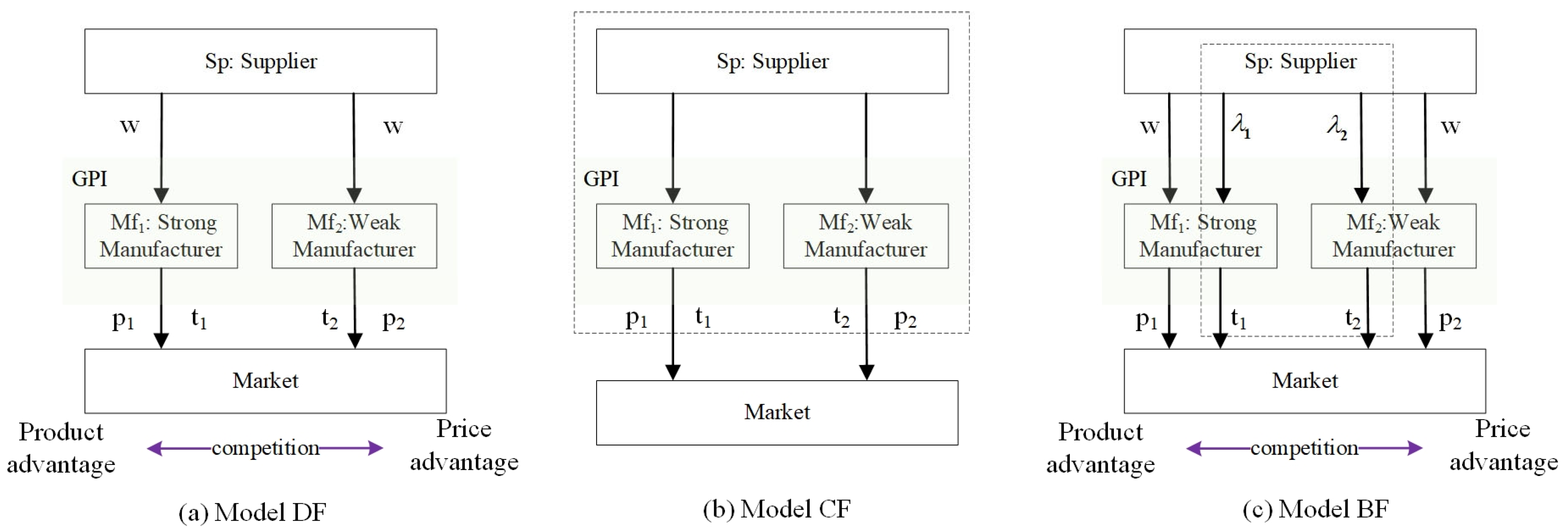
Figure 1. Models DF, CF and BF of the AlBSC.
Sustainability 17 07377 g001
Figure 2. Decision framework of Model BF.
Sustainability 17 07377 g002
Figure 3. The impact of σ on GPI investment.
Sustainability 17 07377 g003
Figure 4. The impact of σ and w on selling prices.
Sustainability 17 07377 g004
Figure 5. The impact of σ on demand.
Sustainability 17 07377 g005
Figure 6. The impact of w on demand.
Sustainability 17 07377 g006
Figure 7. The impact of σ on CS.
Sustainability 17 07377 g007
Figure 8. The impact of σ and μ on λ i .
Sustainability 17 07377 g008
Figure 9. The impact of σ and δ on profit.
Sustainability 17 07377 g009
Figure 10. The impact of σ on SW.
Sustainability 17 07377 g010
Figure 11. The impact of y 1 on profits.
Sustainability 17 07377 g011
Figure 12. The impact of y 1 on GPI investment and SW.
Sustainability 17 07377 g012
Figure 13. The impact of σ and δ on profits.
Sustainability 17 07377 g013
Figure 14. The impact of σ on GPI investment and SW.
Sustainability 17 07377 g014
Figure 15. A strategic managerial decision tree for multi-perspective coordination.
Sustainability 17 07377 g015
Table 1. Summary of reviewed literature.
Ref.Research ObjectSupply Chain StructureCoordinate StrategyMethodsHeterogeneity Setting
[21]Power battery recycling supply chain1 manufacturer, 1 retailerPromotion/wholesale price contractsNon-cooperative gameNo
[22]General supply chain1 manufacturer, 1 retailerRevenue-sharing/cost-sharing contractsNon-cooperative gameNo
[13]Green closed-loop supply chain1 manufacturer, 1 recycler, 1 retailerCooperative allianceCooperative gameNo
[29]General supply chain1 supplier, 2 manufacturersContracts and cooperative gamesNon-cooperative and cooperative gamesNo
[11]Eco-innovation supply chain1 supplier, 2 manufacturersCooperative allianceBiform gameNo
[32]General supply chain1 supplier, 2 manufacturers-Biform gameNo
[37]Low-carbon supply chain1 manufacturer, 1 retailerCooperative allianceBiform gameNo
[40]Retail supply chainDual channels: 1 supplier, 1 retailer-Non-cooperative gameBrand
[41]Retail supply chain2 suppliers, 1 retailer-Non-cooperative gameProduct quality
[42]E-commerce logistics supply chain1 supplier, 2 logistics service providers-Non-cooperative gameBrand
Table 2. Key features of this paper.
ItemSubitemExtant LiteratureThis Paper
2.1 Decision making and coordination of supply chain on green innovationNumber of agents2 or 33
MethodsNon-cooperative game and/or cooperative gameNon-cooperative game and biform game
Number of decision-making methods for contract parameters13 (Section 5)
2.2 The application of biform game in SCMNon-cooperative gameProfit maximization strategiesProfit maximization strategies
Cooperative gameThe core or Shapley valueShapley value
2.3 The operational research on firm heterogeneityHeterogeneous agentsSuppliersManufacturers
Dimensions of heterogeneityProduct, quality or firm abilityInnovation capability
Table 3. Notations of parameters, subscript, superscripts and variables.
CategoryNotionsDescriptions
Parameters a The size of the market for the weak manufacturer, and 0 < a < 1
δ The demand-boosting effect of GPI
σ ICH
μ The cost per unit of GPI for the strong manufacturer
w Wholesale price
Subscript i i { 1,2 } , subscripts 1 and 2 distinguish the two manufactures.
Superscripts D F Decentralized decision making
C F Centralized decision making
B F Biform game-based decision making
P B F Biform game-based decision making under exogenous promotion compensation contract
C P B F Biform game-based decision making under cooperative endogenous promotion compensation contract
D P B F Biform game-based decision making under competitive endogenous promotion compensation contract
Decision variables t i Manufacturer’s GPI efforts
p i Manufacturer’s selling price
λ i Cost-sharing ratio for GPI investment
Variables q i The manufacturer’s market demand
Q Total market demand
π S Supply chain’s profits
π S p Supplier’s profits
π M f i Manufacturer’s profits
C S Consumer surplus
Table 4. Coordination outcomes under different decision-making modes.
How decisions are madeCoordinate the results
ExogenousPareto improvement over Models BF or DF
( Ω 2 : Manufacturer-biased, Ω 3 : Balanced, Ω 4 : Supplier-biased)
Endogenous cooperationPareto improvement over Models BF or DF
(Supplier-biased)
Endogenous competitionNo Pareto improvement
(Manufacturer-biased)
Table 5. The impact of ICH on decisions and coordination.
ModelEnvironmentEconomicsSociety
GPIPricesSupplier’s ProfitManufacturers’ ProfitSupply Chain’s ProfitSW
DF↓↑
CF M f 1 ↑, M f 2 M f 1 ↑, M f 2 ↓↑--
BF M f 1 ↑, M f 2 ↓↑↓↑
Note: ↑ monotonic increase; ↓ monotonic decrease.
Disclaimer/Publisher’s Note: The statements, opinions and data contained in all publications are solely those of the individual author(s) and contributor(s) and not of MDPI and/or the editor(s). MDPI and/or the editor(s) disclaim responsibility for any injury to people or property resulting from any ideas, methods, instructions or products referred to in the content.