Research on the Characteristics and Influencing Factors of Virtual Water Trade Networks in Chinese Provinces

Abstract

Promoting the sustainable development of virtual water trade is of great significance to safeguarding China’s water resource security and balanced regional economic growth. This study analyzes the virtual water trade network among 31 Chinese provinces based on multi-regional input–output tables from 2012, 2015, and 2017, using total trade decomposition, social network analysis, and exponential random graph models. The key findings are as follows: (1) The total virtual water trade volume remains stable, with Xinjiang, Jiangsu, and Guangdong as the core regions, while remote areas such as Shaanxi and Gansu have lower trade volumes. The primary industry dominates, and it is driven by simple value chains. (2) Provinces such as Xinjiang, Heilongjiang, and Jiangsu form the network’s core. Network density and symmetry increased from 2012 to 2015 but declined slightly in 2017, with efficiency peaking and then dropping, and the clustering coefficient decreased annually. Four economic sectors exhibit distinct interactions: frequent two-way flows in Sector 1, significant inflows in Sector 2, prominent net spillovers in Sector 3, and key brokers in Sector 4. (3) The network evolved from a core-periphery structure with weak ties to a stable, heterogeneous, and resilient system. (4) Influencing factors, such asper capita water resources, economic development, and population, significantly impact trade. Similarities in economic levels, population, and water endowments promote trade, while spatial distance has a limited effect, with geographic proximity showing a significant negative impact on long-distance trade.

1. Introduction

In China, the distribution of water resources exhibits a basic pattern:” many people, little water, and abundance in the south and scarcity in the north”. This water resource pattern has become a key factor restricting sustainable economic and social development and the construction of an ecological civilization. The theory of virtual water trade, as an innovative regional water resource allocation strategy, realizes the optimal allocation of water resources in the spatial dimension by embedding water resources into the trade of goods and services in the form of “virtual” resources. In the current national water resource management system, the virtual water mechanism has gradually established its strategic position and become an important policy tool for alleviating conflicts between regional water supply and demand and improving the water resource utilization efficiency.

The construction of a unified national market aims to break the geographical division, promote the free flow and optimal allocation of resource factors, and provide a broad space for the efficient utilization of key production factors, such as water resources. However, the scientific allocation of water resources still faces many difficulties, such as uneven geographical distribution of water resources, low per capita possession, and differences in the efficiency of water resource use and management capacities in different regions. Tony Allan first proposed the concept of “virtual water” in 1997 to characterize the amount of water used in the production of agricultural products [1]. Virtual water refers to the amount of water used in the production and service of a product, and it is characterized by authenticity, convenience, implied value, and social transactions. It can realize the indirect transfer and efficient use of water resources through inter-regional products or service flows and provide new solutions for areas with water shortages. The literature has shown that the net virtual water within China mainly flows from the less developed western regions to the developed coastal regions [2].

In the context of globalized production, it has become common for a product’s different production processes to be distributed in different countries or regions. As a result, intermediate products often cross multiple national borders, which has led to significant double-counting in total trade statistics. This also creates a false impression that the exporting country creates all the value of the exported product. The value added of trade refers to the domestic value incorporated in export products, which measures the economic gains of a country or region participating in the global value chain, i.e., the value created by the production process of export products is decomposed into the countries (or regions) involved, the value produced (created) by the country is accounted for, and the benefits gained by each country in international trade, especially in bilateral trade, are more accurately reflected. Trade value-added accounting is a reconstruction of total trade statistics that objectively reflects the true nature of bilateral trade, while leaving a country or region’s overall trade balance unchanged. American scholars proposed that due to the vertical specialization division of labor in industries and the labor force, etc., the production process of a certain product may span many countries and regions [3]. Based on Koopman’s [3] study, some scholars decomposed total bilateral exports into 16 parts based on the origin of the exported products and the destinations where they were ultimately absorbed, and a new trade statistics rule based on value added was established [4]. Some experts have proposed decomposing a country’s total production activities—at the national, sectorial, or industry-by-country level—into four different types of frameworks: purely domestic demand, traditional international trade, simple Global Value Chain (GVC) activities, and complex GVC activities [5]. Therefore, to advance economic globalization led by China’s domestic demand and promote synergistic and interconnected regional development, it is essential to accelerate the construction and optimization of China’s National Value Chain (NVC) and its division of labor system [6].

Currently, the most mainstream trade accounting method is the input–output analysis method. Some scholars, based on the global multi-regional input–output model (MRIO), have found that developed countries gain significant economic benefits from global trade while bearing low environmental costs. In contrast, developing countries exhibit the opposite phenomenon [7]. By combining the multi-region input–output model to track the implied carbon emissions and value added of six regions from 2010 to 2015, scholars have found that there is a global carbon inequality problem, with major carbon-exporting countries being at a disadvantage in global trade [8]. Researchers have utilized China’s multi-regional input–output tables to track processing exports, demonstrating significant heterogeneity in the nation’s virtual water exports [9,10,11]. Social network analysis has been widely adopted across economic and management research domains. Some scholars have used social network analysis to construct the value-added trade networks of 42 countries from 2008 to 2014, and the impact of trade facilitation on value-added trade networks was investigated from different perspectives [12]. Through the application of social network analysis, scholars have developed network models to examine export trade flows, embedded carbon emissions in exports, domestic value-added contributions, and carbon emissions associated with foreign value-added components. Empirical investigations reveal China’s substantial GVC participation, demonstrating a strategic repositioning from peripheral involvement to a central position within international production networks [13] (Wang et al., 2021).To propel the advancement in carbon neutrality, a group of experts has constructed a sophisticated network model depicting carbon emission transfers within the framework of the global value chain. Through this model, they delved into the pivotal factors influencing such transfers and subsequently formulated a series of effective carbon emission reduction strategies [14]. Some scholars explored the characteristics of virtual water trade networks in 19 major countries between 2006 and 2015, and they found that the density and asymmetry of virtual water trade networks have continued to rise in all industries and in three major industries [15]. Their study shows that in China’s cross-regional and cross-sectoral virtual water trade networks, the most significant virtual water flows are from agriculture to the food industry, and the construction industry has seen a rise in the amount of virtual water due to the growth of domestic demand [16]. With the penetration and integration of the virtual water concept in multiple sectors, it was observed that geospatial proximity, the level of economic development, and openness to the outside world had a positive effect on China’s multi-regional water transfer relationship network [17].

Throughout existing research results, the relevant studies on the network characteristics of virtual water trade in Chinese provinces have become mature, but there is a lack of research on network resilience and influencing factors. Therefore, this study employs a multi-regional input–output framework (MRIO) to systematically assess inter-provincial virtual water transfers across 31 provincial-level administrative units in China. The primary theoretical advancements in this research are threefold: (1) Starting from the perspective of value-added trade, this study not only combines traditional total trade decomposition methods and social network analysis but also introduces a new dimension of structural network resilience analysis in order to comprehensively analyze the characteristics and resilience of virtual water trade transfer networks in each province of China. (2) An advanced exponential random graph model (ERGM) is adopted to explore the impacts of endogenous network structural variables, such as reciprocity in the virtual water trade network, connectivity in the virtual water trade network, and attribute and relational variables such as economic levels and water resource endowments on virtual water trade. These innovations aim to reveal the development status of China’s virtual water trade more realistically and objectively, and the research results have important theoretical value for the scientific cognition of China’s cross-regional water resource allocation efficiency, identifying the stability evolution of the trade network and perfecting the national water resource security strategy. Simultaneously, it is an important tool for constructing a green, low-carbon, and circular economy, which covers the “production–trade–consumption” chain. Moreover, it has significant practical significance for the in-depth coupling of the regional economy and the sustainable development of water resources.

2. Research Methodology and Data Sources

2.1. Multi-Regional Input–Output Modeling

In China’s multi-regional input–output structure, there are m regions and n sectors, with s and r representing exporting and importing regions and i and j representing exporting and importing sectors. x and y are vectors of $mn\times 1$, for which their elements are ${x_i}^s$ and ${y_i}^{sr}$, denoting the output of the sector i in regions due to domestic consumption and the products of the sector i in regions that are finally consumed in region r, respectively. $A$ is a matrix of the direct consumption coefficients of $mn\times mn$, and element ${a_{ij}}^{sr}$ represents the demand of sector i in the regions for the product per unit of the output of sector j in region r. $L=(1-A{)}^{-1}$ is the inverse matrix of Leontief (Leontief). Thus, we have the following:

$$\left[\begin{array}{c}{x}^s\\ x^r\\ ⋮\hfill \\ x^m\end{array}\right]={\left[\begin{array}{c}1-A^{ss}-A^{sr}\cdots -A^{sm}\\ -A^{rs} 1-A^{rr}\cdots -A^{rm}\\ ⋮⋮\ddots ⋮\hfill \\ -A^{ms}-A^{mr}\cdots 1-A^{mm}\end{array}\right]}^{-1}\left[\begin{array}{c}{y}^{ss}+y^{sr}+\cdots y^{sm}\\ y^{rs}+y^{rr}+\cdots y^{rm}\\ ⋮\hfill \\ y^{ms}+y^{mr}+\cdots y^{mm}\end{array}\right]$$

(1)

That is, the simplified formula is as follows:

$$x=(1-A{)}^{-1}y$$

(2)

2.2. Cross-Provincial and Cross-Sectoral Virtual Water Trade Decomposition Models

This study applies the Chinese multi-regional input–output model to study the input–output relationship between different provinces and industries in China. According to the existing literature [4,18,19], the paths in this study are mainly divided in terms of their origins and final absorption destinations; these paths are divided into five parts.

The multi-regional input–output table in China includes n industrial sectors in m provinces, where $W^s$ is the virtual water trade volume of n sectors in s province (n × 1 order), $w^s=W^s/x^s$ is the virtual water trade coefficient vector (n × 1 order), ${\widehat{w}}^s$ is the diagonal matrix of the virtual water trade coefficient of $w^s$ (n × n order), and $L^{ss}=(1-A^{ss}{)}^{-1}$ is the inverse matrix of the Leontief of region s (n × n order), $A^{sr}\mathrm{a}\mathrm{n}\mathrm{d}{ A}^{st}$ are the n-order intermediate demand coefficient matrices of region s to region r and region s to region t, $B^{ru }\mathrm{a}\mathrm{n}\mathrm{d}{B}^{tu}$ are the chunking matrices (n × n order) in the Leontief inverse matrix, and $Y^{ss}$, $Y^{rr}\mathrm{a}\mathrm{n}\mathrm{d}{Y}^{sr}$ are the column vectors of the final demand for the n industry sectors of regions, region r, and region s to region r, respectively (similarly for $Y^{us}$, $Y^{ur}$, etc.).

The decomposition equation of the virtual water trade volume $W^s$ for n sectoral industry levels in province s is as follows:

$$W^s=\underset{W_1}{\underbrace{{\widehat{w}}^s{L}^{ss}{Y}^{ss}}}+\underset{W_2}{\underbrace{{\widehat{w}}^s{L}^{ss}\sum _{\begin{array}{c}r=1\\ r\ne s\end{array}}^G{Y}^{sr}}}+\underset{W_3}{\underbrace{{\widehat{w}}^s{L}^{ss}\sum _{\begin{array}{c}r=1\\ r\ne s\end{array}}^G{A}^{sr}{L}^{rr}{Y}^{rr}}}+\underset{W_4}{\underbrace{{\widehat{w}}^s{L}^{ss}\sum _{\begin{array}{c}r=1\\ r\ne s\end{array}}^G{A}^{sr}\sum _{u=1}^G{B}^{ru}{Y}^{us}}}+\underset{W_5}{\underbrace{{\widehat{w}}^s{L}^{ss}\left(\sum _{\begin{array}{c}r=1\\ r\ne s\end{array}}^G\sum _{\begin{array}{c}t=1\\ t\ne s\end{array}}^G{A}^{st}\sum _{u=1}^G{B}^{tu}{Y}^{ur}-\sum _{\begin{array}{c}r=1\\ r\ne s\end{array}}^G{A}^{sr}{L}^{rr}{Y}^{rr}\right)+\underset{W_6}{\underbrace{{\delta }^s}}}}$$

(3)

Equation (3) represents the decomposition of the virtual water trade at the national sectoral level into five components, which are as follows: W₁ is the amount of virtual water implied in the local demand for final products; W₂ is the amount of virtual water implied in the final demand and exported to other regions; W₃ is the amount of virtual water implied in intermediate products and exported to other regions; W₄ is the amount of virtual water implied in intermediate products that is exported to other regions and then returned to the local area and used to satisfy the local demand for final products; W₅ is the amount of virtual water implicit in intermediate products and re-exported to other regions by the place of import. Since this paper focuses on the 31 provinces of China, Equation (3) disregards the implied value-added W₆ of export products.

According to the number of cross-border trips, region s provides final products, direct intermediates, and indirect intermediates to region r. These are categorized into domestic traditional, simple, and complex trade value chains, which correspond to the second, third, and fifth terms of Equation (3), respectively.

Based on the above and drawing on related studies [19], the formula for the virtual water trade transfer $W^{sr}$ generated by the value-added flow from region s to region r is obtained as follows:

$$W^s=\underset{W_1}{\underbrace{{\widehat{w}}^s{L}^{ss}{Y}^{ss}}}+\underset{W_2}{\underbrace{{\widehat{w}}^s{L}^{ss}\sum _{\begin{array}{c}r=1\\ r\ne s\end{array}}^G{Y}^{sr}}}+\underset{W_3}{\underbrace{{\widehat{w}}^s{L}^{ss}\sum _{\begin{array}{c}r=1\\ r\ne s\end{array}}^G{A}^{sr}{L}^{rr}{Y}^{rr}}}+\underset{W_4}{\underbrace{{\widehat{w}}^s{L}^{ss}\sum _{\begin{array}{c}r=1\\ r\ne s\end{array}}^G{A}^{sr}\sum _{u=1}^G{B}^{ru}{Y}^{us}}}+\underset{W_5}{\underbrace{{\widehat{w}}^s{L}^{ss}\left(\sum _{\begin{array}{c}r=1\\ r\ne s\end{array}}^G\sum _{\begin{array}{c}t=1\\ t\ne s\end{array}}^G{A}^{st}\sum _{u=1}^G{B}^{tu}{Y}^{ur}-\sum _{\begin{array}{c}r=1\\ r\ne s\end{array}}^G{A}^{sr}{L}^{rr}{Y}^{rr}\right)+\underset{W_6}{\underbrace{{\delta }^s}}}}$$

(4)

Similarly, the virtual water trade transfer $W^{rs}$ from region r to region s can be calculated. From this, the bilateral net virtual water trade transfer $\mathsf{\Delta }{W}^{sr}$ from region s to region r can be calculated as follows:

$$\mathsf{\Delta }{W}^{sr}=W^{sr}-W^{rs}$$

(5)

As can be seen from the above equation, $\mathsf{\Delta }{W}^{sr}=-\mathsf{\Delta }{W}^{rs}$. If $\mathsf{\Delta }{W}^{sr}>0$, this means that region s is in the net virtual water outflow position in the trans-regional value-added flow between region sand region r. Along with the value-added flow, region s provides a portion of virtual water to region r and vice versa.

2.3. Social Network Analysis Methods

As a practical method based on the cross-fertilization of multiple disciplines—such as mathematics, management, sociology, psychology, and statistics—social network analysis is widely used in political, academic, and economic circles. In layman’s terms, a social network is a collection of multiple points (the individuals of the study object) and the connecting lines between the points (the relationships between the individuals of the study object). In this study, 31 provinces in China are used as nodes, and the virtual water transfer relationships between provinces are used as edges to construct a virtual water transfer relationship network G = (M, P, W) for the 31 provinces in China, where M denotes the set of vertices of the network, P denotes the set of edges, and W is the set of weights.

We define the adjacency matrix of network $H=\left(h_{ij}\right)$ to represent the virtual water transfer relationship between the provinces in the network. When the virtual water transfer from province $i$ to $j$ is strictly greater than the average of the total amount of transfer from each province, there exists an edge $p_{ij}$ pointed by node $i$ to node $j$. In this case, $h_{ij}=1$; otherwise, $h_{ij}=0 (i,j=1, 2,\cdots , 31)$. The weight $w_{ij}$ of the edge ${ p}_{ij}$ takes the value of the virtual water transfer from province $i$ to $j$.

2.3.1. Indicators Related to the Overall Characteristics of the Network

According to the existing research, the overall characterization of the network was selected to portray four indicators: network density, symmetry, clustering coefficient, and average path length of the virtual water trade network [20].

• Network Density

Network density is the ratio of the number of edges that are actually present to the maximum number of edges possible, and it is used to measure the closeness of network connections. Denoting the number of edges in the network by $\left|P\right|$ and letting n be the number of nodes in the network, the network density U is calculated as follows:

$$U={\displaystyle \frac{\left|P\right|}{n(n-1)}}$$

(6)

2.

Symmetry (Reciprocity)

Symmetry is commonly used in directed networks to measure the degree of interconnection between two nodes in the network. It is mainly quantified by the reciprocity coefficient. A directed edge pointing from node X to node Y is randomly selected in a directed network, and the probability of the existence of a directed edge pointing from node Y to node X is computed, where R denotes the number of edges of the reversed edge, and symmetry is computed via the following formula:

$$\phi ={\displaystyle \frac{R}{\left|P\right|}}$$

(7)

3.

Average Clustering Coefficient

The clustering coefficient refers to the degree of interconnection between neighboring nodes of a node, and itis used to measure the aggregation degree of nodes in our virtual water transfer network. The global clustering coefficient (GC) is computed by averaging the local clustering coefficients of every node. Node ${ m}_i$ has ${ k}_{i }$ neighboring nodes, and the number of edges connected to the neighboring nodes is $P_i$; then, the clustering coefficient $G{C}_i$ of node ${ m}_i$ and the average clustering coefficient $GC$ are calculated via the following formula:

$$G{C}_i={\displaystyle \frac{P_i}{k_i(k_i-1)}}$$

(8)

$$GC={\displaystyle \frac{\sum G{C}_i}{n}}$$

(9)

4.

Average Path Length

The average path length is used to measure the virtual water transfer efficiency of our virtual water transfer network by calculating the average value of the shortest path between nodes in the network. The smaller the average path length, the more convenient and close the connection between a certain node. Using $d_{ij}$ to denote the weighted shortest path length between nodes $m_i$ and $m_j$, the average path length GL is calculated as follows:

$$GL={\displaystyle \frac{{\sum }_{i,j}{d}_{ij}}{n(n-1)}}$$

(10)

2.3.2. Indicators Related to Individual Characteristics of the Network

According to the existing research, the individual characteristics of the network are portrayed by three indexes: point centrality, proximity centrality, and intermediate centrality of the virtual water trade network [20].

• Degree Centrality

Degree centrality is the number of points directly connected to a node; it is an important indicator of the centrality, importance, and activity of a node in the network. In directed graphs, it is equal to the sum of out-degree centrality and in-degree centrality, where out-degree centrality is the number of edges directed from the node to other nodes, and in-degree centrality is the number of edges directed to the node from other nodes. Nodes with high degree centrality usually occupy a core position in the network, and they have more connectivity and greater influence. In China’s virtual water transfer network, the outgoing degree centrality ${{ d}_i}^{out}$ and incoming degree centrality ${{ d}_i}^{in}$ of node $m_i$ reflect the number of virtual water outflow and inflow relationships from province i to other provinces, respectively, and the sum of outgoing and incoming degrees is recorded as $d_i$. Considering the effect of weights, the weighted outward centrality ${w_i}^{out}$ and weighted inward centrality ${{ w}_i}^{in}$ of node $m_i$ are defined as the virtual water outflow and inflow transfers from province $i$ to other provinces, and the sum of weighted outward centrality and weighted inward centrality is denoted as ${ w}_i$:

$${d_i}^{out}=\sum _{P_{ij}\in P}{h}_{ij},{d_i}^{in}=\sum _{P_{ij}\in P}{h}_{ji}$$

(11)

$${w_i}^{out}=\sum _{P_{ij}\in P}{w}_{ij},{w_i}^{in}=\sum _{P_{ij}\in P}{w}_{ji}$$

(12)

$$d_i={d_i}^{out}+{d_i}^{in},w_i={w_i}^{out}+{w_i}^{in}$$

(13)

2.

Closeness Centrality

Closeness centrality is the sum of the shortest path distances of a particular node from all other nodes in the network, and it is used to measure the degree to which a particular node is not controlled by others. If the distance between a node and all other nodes in the network is very short, this means that the node has a high closeness centrality. In our virtual water transfer network, a higher closeness centrality value indicates that a province is farther from the core of the network and has a weaker influence in terms of resources, rights, and other aspects. Assuming that ${d_i}^{short}$ is the length of the shortcut between node $m_i$ and other nodes, the formula for calculating the closeness centrality $P{C}_i$ of node ${ m}_i$ is as follows:

$$P{C}_i={\displaystyle \frac{n-1}{\sum {d_i}^{short}}}$$

(14)

3.

Betweenness Centrality

The betweenness centrality portrays the strength of the research individual’s control over resources. If a node is located on the shortest path (shortcut) of many other pairs of points, this means that the point has a high betweenness centrality, and the corresponding province of this node plays a strong mediating role in the virtual water transfer network of our country. To calculate the probability that node $m_{i }$ is on a shortcut between nodes $m_i$ and ${ m}_k$, such that the number of shortcuts that exist between nodes ${ m}_j$ and $m_k$ is ${ g}_{jk}$, and the number of shortcuts proceeding through the node $m_i$ and connecting nodes $m_{j }$ and ${ m}_k$ is ${ g}_{jk}\left(i\right), j\ne k\ne i$, the betweenness centrality $I{C}_i$ of node $m_i$ is calculated via the following formula:

$$I{C}_i={\displaystyle \frac{2{\sum }_j{\sum }_k\frac{g_{jk}\left(i\right)}{g_{jk}}}{n^2-3n+2}}$$

(15)

2.3.3. Block Model Analysis

White proposed the block model theory as early as 1976, which divides individual nodes into blocks based on structural information, focusing mainly on the relationship between individual locations rather than the research object itself [20]. Firstly, the iterative correlation convergence method CONCOR (convergent correlations) is utilized to partition each province corresponding to the virtual water transfer network in China according to its structural similarity; this is carried out to simplify the data. Then, each Chinese province’s network position is assessed using virtual water flow data, considering transfers both within and across segments.

Assuming that the number of provinces included in plate q is ${ S}_q$, the total number of possible relationships included within plate q is $S_q(S_q-1)$, a total of $S$ provinces are included in our virtual water transfer network, and there is $S_q\left(S-1\right)$ for all possible relationships for each member of plate q. Therefore, the expected proportion of virtual water transfer relationships within plate q as a p of the whole can be derived as ${\displaystyle \frac{S_q(S_q - 1)}{S_q(S - 1)}}={\displaystyle \frac{(S_q - 1)}{(S - 1)}}$. Combined with the calculated expected proportion, the virtual water transfer network in China can be categorized into four location relationship types, as shown in

Table 1. Classification method for positional relationships in the global virtual water trade net transfer network.

Proportion of Intra-Plate Relationships	Ratio of Virtual Water Outflow to Inflow Relationship between the Plate and the External Plate
	≥1	<1
$⩾{\displaystyle \frac{(S_q-1)}{(S-1)}}$	Two-way spillover plates	Main beneficiary sectors
$<{\displaystyle \frac{(S_q-1)}{(S-1)}}$	Net overflow sector	Brokerage board

.

2.3.4. Methods for Assessing Network Structural Resilience

Based on existing research, this study comprehensively measures the structural resilience of virtual water transfer relationship networks in 31 provinces of China through the following indicators [21,22,23,24]:

• Clustering: Average clustering coefficient; see Equations (8) and (9) for details.
• Transmissibility: Average path length; see Equation (10) for details.
• Hierarchical Nature: Degree distribution.

The hierarchical nature of the network structure is mainly expressed through the network degree distribution, and the slope of the degree distribution is positively correlated with the hierarchical nature among the nodes. The larger the slope, the more obvious the hierarchical nature and the more stable the network structure. Hierarchical structure can be measured using the probability distribution of the degree of each node within the network. Using the degree value of the node to draw a power law curve, the degree distribution of the formula is as follows:

$$\mathit{ln}(w_i)=\mathit{ln}(C)+\alpha \mathit{ln}({w_i}^{\mathrm{*}})$$

(16)

Here, $w_i$ denotes the total degree (sum of in-degree and out-degree) of node i, and ${w_i}^{\mathrm{*}}$ represents its rank-ordered degree (nodes sorted by descending degree). C is a proportionality constant. $\alpha$ is the slope ofthe curve of the degree distribution, and the magnitude of $\alpha$ is directly proportional to the hierarchical structure.

4.

Matchability: Degree correlation.

Matchability reflects the tendency to establish trade relationships between individuals in a trade network. This tendency is mainly categorized into matchability and non-matchability. Matchability refers to the tendency of nodes in a network to establish trade relationships with nodes that are similar to their own strength (the number of trade relationships they already have). Non-matchability refers to the tendency of nodes in the network to establish trade relations with some nodes directly connected to node $i$. It is first calculated as $\overline{W_i}$. Then, the linear relationship between degrees $w_i$ and $\overline{{ W}_i}$ of node $i$ is estimated as a curve:

$$\overline{W_i}={\displaystyle \frac{{\sum }_{i\in V}^n{w}_h}{w_i}}$$

(17)

$$\overline{W_i}=D+b{w}_i$$

(18)

Here,${ w}_h$ is the degree of the neighboring node h of node $i$. V is the set of all neighboring nodes of node $i$. D is a constant. bis a coefficient that measures the size of the degree correlation change. When b < 0, the network is designated as non-matching, which indicates that nodes with higher degrees tend to be connected to nodes with lower degrees of connectivity. When b > 0, the network is designated as matching, which indicates that nodes with higher degrees tend to be connected to nodes with similar degrees of connectivity, and the absolute value of b can be used to measure the strength of network matching.

5.

Network Structural Resilience Index.

In this study, agglomeration, transferability, hierarchy, and matching indicators are selected to comprehensively measure the network structural resilience of virtual water transfer relationships in 31 provinces of China [21]. This study considers these four indicators to have the same effectiveness with respect to network structural resilience; thus, the weight of each indicator is set to 0.25, and the formula for calculating the network structural resilience of virtual water transfer relationships in China’s 31 provinces is as follows:

$$K=\sum _{i=1}^4{Z}_i{I}_i$$

(19)

Here, K is the network structural resilience index, ${ Z}_i$ is the weight of thei-th indicator, and $I_{i }$ is the value of thei-th indicator.

6.

Network Resilience Structural Determination.

Combining hierarchical and matching properties, network structural resilience is classified into three categories, as shown in

Table 2. Types of network structural resilience.

Typology	Randomized Network T1	Isomorphic Core–Edge Network T2	Resilience Network T3
Distribution degree	$\left|\alpha \right|\approx 0$	$\left|\alpha \right|>0$	$\left|\alpha \right|>0$
Association characteristics	The network structure is flat and resistant to external damage, but it lacks cohesion and core points.	The network structure is three-dimensional and cohesive, but the phenomenon of homogeneous clustering is significant and tends to weaken the resilience of the network structure.	The network structure is more resilient, and innovative behavior can easily spread from peripheral to core members.

.

2.4. Exponential Random Graph Model

An exponential random graph is a statistical framework for analyzing network data that describes the probability of connections between network nodes by means of an exponential function form. The model is capable of capturing complex dependencies in networks and is widely used in social network analysis [25,26,27,28,29,30].

The standard form of a known directed ERGM model is as follows:

$$\mathit{Pr}\left(\left.Y=y\right|\theta \right)=P_{\theta }\left(y\right)={\displaystyle \frac{1}{l_{\theta }}}\mathit{exp}\left\{{\theta }_a^T{Z}_a\left(y\right)+{\theta }_b^T{Z}_b\left(y,m\right)+{\theta }_c^T{Z}_c\left(y,n\right)\right\}$$

(20)

Equation (20) represents the probability of the occurrence of the observed network structure y given the model parameter θ, where ${ Z}_a\left(y\right)$ is an endogenous network structure variable used to capture dependencies and structural effects in the network, describing how the connectivity patterns in the network y are affected by the network’s own structure, e.g., reciprocity, transitivity, etc. $Z_b\left(y,m\right)$ denotes information about actor attributes associated with network nodes that can influence the pattern of connectivity and strength of relationships between nodes, e.g., level of economic development, population size, etc. [31]. $Z_c\left(y,n\right)$ denotes exogenous network covariates that are not influenced by the internal structure of the network but are determined by factors external to the network, such as the distance factor. ${ \theta }_a,{\theta }_b,{\mathrm{a}\mathrm{n}\mathrm{d} \theta }_c$ indicate the magnitude and direction of the influence of each network statistic on the network, respectively.

The simplification of Equation (20) yields the following general form of ERGM:

$$\mathit{Pr}\left(\left.Y=y\right|\theta \right)=P_{\theta }\left(y\right)={\displaystyle \frac{1}{l_{\theta }}}\mathit{exp}\left\{{\theta }_1{Z}_1\left(y\right)+{\theta }_2{Z}_2\left(y\right)+\dots +{\theta }_p{Z}_p\left(y\right)\right\}$$

(21)

The ERGM model employs Markov chain Monte Carlo maximum likelihood estimation (MCMC MLE), which aims to achieve a high degree of matching between the simulated and observed networks through a continuous simulation process and parameter adjustment strategy. This method can properly handle complex and interdependent relationships among observations, effectively avoiding the difficulties of heteroscedasticity, autocorrelation, and endogeneity, which are often encountered in traditional econometric regression models, thus ensuring the reliability and stability of the analysis results. In addition, the ERGM model can be constructed and estimated with the help of the Stat net module in R software, and the Akaike Information Criterion (AIC) and Bayesian Information Criterion (BIC) are used as assessment tools to evaluate the model’s goodness-of-fit and simplicity [32].

This study employs an exponential random graph model (ERGM) to identify the factors influencing China’s annual virtual water trade networks in 2012, 2015, and 2017. The ERGM framework simulates the effects of both internal and external factors on the formation of virtual water trade transfer networks by integrating endogenous structure, actor attribute variables, and exogenous network covariates. The ERGM statistics are shown in

Table 3. Explanation of ERGM variables.

Variable Type	Statistical Measure	Explanation
Endogenous Network Variables	Edges	Serves as the constant term, not interpreted
	Mutual	Tendency to form mutually interactive trade relationships
	Two path	Whether a node region has many outgoing and incoming relationships
	Balance	Whether the relationship patterns in the network conform to an expected consistency or stability level
	Gwesp	Phenomenon where nodes tend to form tightly connected clusters or cliques
Actor Attribute Variables	Sender-nodeocov	Tendency for provinces with certain attributes to become senders
	Receiver-nodeicov	Tendency for provinces with certain attributes to become receivers
	Absdiff	Tendency for network relationships to form between provinces with dissimilar attributes
Exogenous Network Covariates	Edgecov	Influence of external environmental factors on the formation of virtual water trade networks

.

Based on existing studies, this study selects edges, mutual, balance, and gwesp as endogenous network structure indicators to observe the impact of the network’s own structure on the virtual water trade transfer network. Considering the influence of economic level, population flow, and water resource volume on the overall development of each region, economic development level (gdp), population volume level (popu), and per capita water resource possession (pwater) are selected as explanatory variables, and three actor attributes, namely, the sender effect (sender), the receiver effect (receiver), and the anisotropy (absdiff), are used as explanatory variables for systematic research. Since geographic distance has a strong impact on regional trade development, the geographic proximity network (D[0,500], D[500,1000], D[1000,1500], D[1500,2000]) and the spatial distance network (spadis) were selected as exogenous network covariates [33,34].

Based on the content of the aforementioned formula, the specific form of the ERGM model for this study is obtained as follows:

$$P_{\theta }\left(y\right)={\displaystyle \frac{1}{l_{\theta }}}\mathit{exp}\left\{\begin{array}{c}{\theta }_a^T{Z}_a\left(y\left(edges,mutual,twopath,balance,gwesp\right)\right)+\\ {\theta }_b^T{Z}_b\left(y,m\left(gdp,popu,pwater\right)\right)+\\ {\theta }_c^T{Z}_c\left(y,n\left(D\left[0-500\right],D\left[500-1000\right],D\left[1000-1500\right],D\left[1500-2000\right],spadis\right)\right)\end{array}\right\}$$

(22)

2.5. Datasources

This paper’s research data mainly covers the years 2012, 2015, and 2017. This study primarily utilizes China’s multi-regional input–output (MRIO) tables for 2012, 2015, and 2017, which were obtained from the China Carbon Accounting Database (CEADs), alongside corresponding data from the China Statistical Yearbook. Due to compilation complexities, China’s multi-regional input–output tables are currently only available up to 2017. These time periods coincided with major adjustments in the global trade pattern and the recovery phase following the international financial crisis. During this time, China’s economy gradually transitioned from high-speed growth to medium-high-speed growth and began to focus more on the quality and efficiency of economic development. The mechanism for collecting and releasing relevant data was relatively mature during this period, and the officially released data had a high degree of continuity and consistency, allowing access to relatively complete, stable, and high-quality data. Between 2012 and 2017, the Chinese government introduced important policies on environmental protection, energy conservation, and emission reduction. Examples include the 2013 Action Plan for the Prevention and Control of Air Pollution and the Green Manufacturing Concept of Made in China 2025, introduced in 2015. 2016 marked the beginning of the 13th Five-Year Plan, which emphasized green development and ecological civilization goals and guided the economic development model and environmental protection strategy in subsequent years. This plan emphasizes green development and ecological civilization construction goals, which guide the economic development model and environmental protection strategy in subsequent years. Around 2017, construction of China’s carbon trading market accelerated, and some provinces and cities started piloting carbon emissions trading. During this period, the Chinese government also launched a series of regional development strategies, such as the “Belt and Road” initiative and the development of the Yangtze River Economic Belt. Implementing these strategies and policies has had a far-reaching impact on value chain integration and regional carbon emissions. This study covers all 31 Chinese provinces, consolidating the original 42 sectors into 3 aggregated sectors: agriculture, industry, and services. According to the essential characteristics of economic activities, the rules of consolidation are as follows: agriculture is engaged in the production of primary agricultural products; industry is centered on processing raw materials and manufacturing products; and services provide non-material production services. This is in line with the basic logic of the industrial division of the national economy. Thus, the agricultural sector is directly categorized as agriculture; the remaining 39 sectors, ranging from coal mining to water production and supply, are unified into the industrial category; and the last four sectors—construction, wholesale and retail trade, transportation and storage, and postal services—are grouped into the services category. Supplementary variables were sourced from the China Water Resources Bulletin, China Population and Employment Statistics Yearbook, China Labor Statistics Yearbook, and corresponding provincial statistical yearbooks.

3. Results and Discussion

3.1. Measurement of China’s Inter-Provincial Virtual Water Trade and Analysis of Results

3.1.1. Analysis of the Results of China’s Inter-Provincial (Industry) Virtual Water Trade

(1) Analysis of inter-provincial virtual water trade results

As observed in Figure 1, the total virtual water trade of 31 provinces in China remained relatively stable in 2012, 2015, and 2017, fluctuating between 494.1 billion and 509.9 billion cubic meters. During this period, Xinjiang occupied the top of the list for total virtual water trade, with an average value of 46.019 billion cubic meters, accounting for about 9.2%. This is closely related to its positioning as a national, high-quality cotton production base. Through agricultural subsidies, irrigation facility investments, and other policies, the state ensures the production and output scale of cotton and other agricultural products that require large amounts of water, despite the relative scarcity of local water resources. This supports a sustained huge virtual water outflow. Jiangsu, Guangdong, and other economically developed regions with relatively abundant water resources generally have higher total virtual water trade, showing the activity and influence of these regions in the water resource market. Heilongjiang, Hunan, and Hubei are also prominent in the virtual water trade due to their developed agriculture and abundant water resources. Among them, Heilongjiang’s outstanding performance is attributed to improvements in grain logistics infrastructure and the strategy of strengthening the agricultural province. As an important grain production region, the province’s corn, soybean, and other grain output is accompanied by a large amount of virtual water flow. The well-developed warehousing and railroad transportation networks improve the efficiency of cross-regional deployment. Superimposed on the national food security policy, the province is able to maintain a significant volume of virtual water trade during its economic transition. Simultaneously, the total volume of trade in “Shaanxi, Gansu, Ningxia, and Tibet” is relatively low due to multiple factors, such as geographic location, climatic conditions, industrial structure, and policy orientation. Beijing and Tianjin, on the other hand, have a low volume of virtual water trade due to the relative scarcity of water resources and high demand for water resources due to their developed economies. In these three years, the sum of the average virtual water trade of Qinghai, Beijing, and Tianjin accounted for about 1.54%, which is only 1/6 of that of Xinjiang.

(2) Analysis of the results of the virtual water trade in three industries

As observed in Figure 2, between 2012 and 2017, the virtual water trade volume of the primary industry always occupied an absolutely dominant position, far exceeding that of the secondary and tertiary industries, reflecting the central role of agriculture in China’s water consumption and trade. Simultaneously, the virtual water trade volume of the secondary industry, though not as large as that of the primary industry, also occupies a considerable share, and its change shows a trend that first decreased and then increased. In contrast, the virtual water trade volume of the tertiary industry is always at the lowest level and shows an increasing trend year by year. The formation of these characteristics and changing trends is caused by multiple reasons. Firstly, the year-on-year increase in the virtual water trade volume of the primary industry may be closely related to the acceleration of agricultural modernization and the scaling-up of agricultural production. Secondly, the initial decline followed by a subsequent increase in the virtual water trade volume of the secondary industry may be related to the adjustment of industrial structures, the strengthening of the water resource management policy, and the promotion of water-saving technology. Finally, the rising virtual water trade in services is associated with accelerated sectoral development, optimized industrial structure, and improved water resource utilization efficiency.

3.1.2. Analysis of Net Virtual Water Trade Flows Between Chinese Provinces Along the Three Major Value Chains

As observed in

Table 4. Net flows of virtual water trade among Chinese provinces on three major value chains in 2012.

Province	Traditional Value Chain			Simple Value Chain			Complex Value Chain
	Inflow	Outflow	Net flow	Inflow	Outflow	Net flow	Inflow	Outflow	Net flow
Beijing (BJ)	58.781	17.253	−41.528	47.923	12.835	−35.088	64.732	7.670	−57.062
Tianjin (TJ)	45.427	13.302	−32.125	34.972	14.017	−20.955	41.734	4.191	−37.543
Hebei (HB)	98.924	104.665	5.741	116.723	126.800	10.077	41.019	56.405	15.386
Shanxi (SX)	68.857	56.043	−12.815	56.556	50.410	−6.145	25.781	10.058	−15.723
Inner Mongolia (NM)	89.779	82.992	−6.787	103.048	116.024	12.977	37.639	52.991	15.352
Liaoning (LN)	97.825	93.142	−4.683	145.973	119.664	−26.309	56.498	25.222	−31.276
Jilin (JL)	70.663	82.028	11.364	95.244	107.594	12.351	19.190	30.205	11.015
Heilongjiang (HLJ)	153.017	203.846	50.829	110.760	162.396	51.636	33.318	106.457	73.139
Shanghai (SH)	176.912	65.609	−111.303	75.216	56.468	−18.748	62.774	17.444	−45.330
Jiangsu (JS)	267.540	321.857	54.317	400.823	407.721	6.897	73.200	85.873	12.673
Zhejiang (ZJ)	149.166	118.312	−30.855	154.229	117.778	−36.451	74.820	24.642	−50.178
Anhui (AH)	99.107	143.304	44.197	125.580	160.826	35.245	41.648	101.512	59.864
Fujian (FJ)	136.284	128.511	−7.774	172.659	165.051	−7.607	30.830	15.851	−14.979
Jiangxi (JX)	118.242	142.257	24.015	175.101	198.932	23.832	23.971	64.642	40.671
Shandong (SD)	179.849	135.787	−44.062	389.632	270.415	−119.217	149.122	20.362	−128.760
Henan (HEN)	128.577	133.562	4.986	216.216	216.855	0.638	69.466	66.678	−2.788
Hubei (HUB)	235.035	248.496	13.461	389.360	383.632	−5.728	28.207	18.837	−9.370
Hunan (HUN)	177.097	212.219	35.122	247.200	283.853	36.654	27.280	81.339	54.059
Guangdong (GD)	413.602	318.695	−94.907	321.388	250.157	−71.231	134.277	23.099	−111.178
Guangxi (GX)	174.963	198.810	23.847	195.224	225.718	30.495	23.702	65.422	41.720
Hainan (HN)	22.014	23.349	1.335	13.137	17.147	4.010	10.255	15.832	5.577
Chongqing (CQ)	49.510	52.075	2.565	59.160	55.816	−3.344	26.763	22.089	−4.674
Sichuan (SC)	189.261	196.732	7.471	288.370	285.903	−2.466	28.667	24.851	−3.816
Guizhou (GZ)	58.131	59.224	1.092	51.545	60.985	9.440	14.028	27.524	13.496
Yunnan (YN)	111.077	108.010	−3.067	93.026	96.421	3.395	29.688	29.075	−0.613
Xizang (XZ)	27.531	26.588	−0.943	15.386	14.200	−1.187	2.911	0.603	−2.308
Shaanxi (SHX)	46.923	42.679	−4.244	45.506	42.038	−3.468	37.227	26.375	−10.853
Gansu (GS)	55.044	69.823	14.779	50.985	66.798	15.813	12.294	36.091	23.797
Qinghai (QH)	21.655	20.964	−0.691	13.773	14.540	0.768	3.454	3.847	0.393
Ningxia (NX)	45.064	48.876	3.812	40.075	43.384	3.309	5.520	10.745	5.225
Xinjiang (XJ)	227.597	324.445	96.848	218.163	318.573	100.410	18.033	172.116	154.083
Total flow	3793.453			4462.953			1248.048

,

Table 5. Net flows of virtual water trade among Chinese provinces on three major value chains in 2015.

Province	Traditional Value Chain			Simple Value Chain			Complex Value Chain
	Inflow	Outflow	Net flow	Inflow	Outflow	Net flow	Inflow	Outflow	Net flow
Beijing (BJ)	36.653	28.792	−7.861	35.830	11.178	−24.652	50.981	8.686	−42.295
Tianjin (TJ)	38.721	12.885	−25.836	32.452	13.383	−19.069	43.729	7.153	−36.576
Hebei (HB)	99.621	102.851	3.230	95.775	106.673	10.898	42.430	67.612	25.181
Shanxi (SX)	59.599	49.840	−9.759	53.793	49.226	−4.567	30.398	19.401	−10.997
Inner Mongolia (NM)	72.007	70.572	−1.435	92.874	116.973	24.100	31.715	82.186	50.470
Liaoning (LN)	79.989	83.730	3.742	124.781	125.160	0.379	41.998	43.164	1.165
Jilin (JL)	71.316	78.889	7.573	81.871	97.900	16.029	22.196	44.899	22.703
Heilongjiang (HLJ)	128.281	185.085	56.805	89.058	154.771	65.713	324.544	161.854	−162.690
Shanghai (SH)	112.159	46.549	−65.610	66.042	60.064	−5.978	40.920	31.121	−9.798
Jiangsu (JS)	252.299	330.104	77.805	360.704	382.343	21.639	84.299	145.060	60.761
Zhejiang (ZJ)	135.719	114.658	−21.061	148.086	93.970	−54.117	105.453	29.129	−76.324
Anhui (AH)	138.361	150.957	12.597	132.385	133.722	1.337	82.710	120.554	37.844
Fujian (FJ)	112.424	111.457	−0.967	141.792	142.214	0.422	32.087	43.727	11.640
Jiangxi (JX)	139.945	152.132	12.187	153.367	167.185	13.818	34.910	78.131	43.221
Shandong (SD)	155.433	135.388	−20.046	279.092	222.643	−56.449	90.652	30.203	−60.449
Henan (HEN)	137.133	128.585	−8.548	195.773	168.882	−26.891	105.592	78.946	−26.646
Hubei (HUB)	262.540	261.564	−0.977	316.568	288.149	−28.419	62.822	28.705	−34.117
Hunan (HUN)	196.092	220.048	23.957	206.553	233.350	26.797	41.933	98.328	56.395
Guangdong (GD)	397.924	286.825	−111.098	298.440	218.903	−79.537	157.331	51.291	−106.039
Guangxi (GX)	166.578	188.983	22.405	156.541	190.960	34.419	29.130	95.728	66.598
Hainan (HN)	19.875	21.755	1.880	11.842	16.571	4.729	11.792	22.490	10.698
Chongqing (CQ)	79.474	54.879	−24.595	61.239	33.812	−27.426	62.626	17.763	−44.863
Sichuan (SC)	208.129	218.568	10.439	268.455	262.733	−5.721	37.906	33.540	−4.366
Guizhou (GZ)	62.496	62.370	−0.126	36.303	41.046	4.743	21.878	31.827	9.949
Yunnan (YN)	113.570	104.612	−8.958	77.550	71.877	−5.673	46.057	32.952	−13.105
Xizang (XZ)	28.483	27.149	−1.333	9.989	10.228	0.239	1.989	2.192	0.203
Shaanxi (SHX)	53.102	46.297	−6.805	41.900	40.314	−1.586	42.708	39.091	−3.617
Gansu (GS)	53.327	67.451	14.125	42.210	56.331	14.122	16.754	47.744	30.990
Qinghai (QH)	27.139	22.199	−4.940	12.307	11.486	−0.821	5.708	3.977	−1.731
Ningxia (NX)	48.304	50.927	2.623	34.582	36.251	1.669	7.878	13.448	5.570
Xinjiang (XJ)	251.521	322.109	70.588	166.100	265.952	99.852	21.608	221.832	200.224
Total flow	3738.210			3824.249			1732.734

and

Table 6. Net flows of virtual water trade among Chinese provinces on three major value chains in 2017.

Province	Traditional Value Chain			Simple Value Chain			Complex Value Chain
	Inflow	Outflow	Net flow	Inflow	Outflow	Net flow	Inflow	Outflow	Net flow
Beijing (BJ)	51.839	14.189	−37.650	29.533	9.188	−20.345	50.791	7.184	−43.607
Tianjin (TJ)	23.528	13.334	−10.194	24.672	13.156	−11.515	21.652	4.663	−16.989
Hebei (HB)	106.929	110.294	3.365	130.652	127.485	−3.167	50.481	44.050	−6.431
Shanxi (SX)	90.025	58.736	−31.289	53.525	39.905	−13.620	35.042	9.690	−25.351
Inner Mongolia (NM)	89.156	104.139	14.983	56.934	73.422	16.488	26.951	50.083	23.132
Liaoning (LN)	86.741	79.047	−7.693	69.181	65.475	−3.706	38.756	32.079	−6.677
Jilin (JL)	47.393	63.524	16.131	62.707	65.159	2.453	37.106	47.263	10.157
Heilongjiang (HLJ)	113.946	161.704	47.757	109.767	159.784	50.016	31.119	160.906	129.788
Shanghai (SH)	62.722	46.402	−16.320	37.039	43.991	6.952	27.750	33.360	5.610
Jiangsu (JS)	320.543	339.320	18.777	495.265	509.970	14.705	91.553	121.082	29.530
Zhejiang (ZJ)	139.257	99.254	−40.003	137.787	94.268	−43.520	112.690	35.438	−77.251
Anhui (AH)	161.715	191.790	30.075	243.301	253.034	9.733	44.630	62.130	17.501
Fujian (FJ)	144.273	133.159	−11.113	189.669	174.352	−15.317	42.327	24.252	−18.075
Jiangxi (JX)	132.866	143.558	10.692	155.218	174.947	19.728	36.320	69.542	33.221
Shandong (SD)	146.763	133.789	−12.975	314.123	292.700	−21.424	59.378	22.559	−36.819
Henan (HEN)	147.691	140.835	−6.856	211.536	192.025	−19.510	100.574	55.476	−45.098
Hubei (HUB)	254.886	242.423	−12.464	381.535	363.640	−17.896	50.687	24.778	−25.910
Hunan (HUN)	235.350	246.276	10.926	310.229	314.046	3.817	52.040	55.810	3.770
Guangdong (GD)	279.545	247.738	−31.807	241.957	223.876	−18.081	117.185	74.802	−42.383
Guangxi (GX)	163.906	191.951	28.045	157.176	174.268	17.093	32.943	58.635	25.692
Hainan (HN)	24.357	24.313	−0.045	9.155	13.849	4.694	9.131	15.317	6.186
Chongqing (CQ)	65.087	46.938	−18.149	52.782	37.404	−15.377	49.107	18.956	−30.151
Sichuan (SC)	217.162	222.389	5.226	305.724	287.951	−17.773	54.426	27.705	−26.721
Guizhou (GZ)	73.360	61.334	−12.026	46.143	47.507	1.364	29.681	29.165	−0.516
Yunnan (YN)	107.430	107.465	0.035	112.147	105.714	−6.433	51.293	31.001	−20.292
Xizang (XZ)	28.987	28.211	−0.776	12.941	11.353	−1.588	4.502	1.760	−2.742
Shaanxi (SHX)	59.612	42.980	−16.632	51.941	41.448	−10.493	54.953	38.213	−16.740
Gansu (GS)	67.858	70.250	2.392	49.957	58.869	8.912	15.007	34.529	19.522
Qinghai (QH)	18.287	17.955	−0.332	21.296	21.763	0.467	5.187	5.427	0.240
Ningxia (NX)	45.250	42.990	−2.260	38.731	39.535	0.804	11.289	10.246	−1.042
Xinjiang (XJ)	243.186	323.364	80.178	195.972	278.509	82.538	31.031	169.477	138.446
Total flow	3749.648			4308.591			1375.578

, in the years 2012, 2015, and 2017, China’s virtual water flows exhibited significant value chain differences. The simple value chain accounted for the largest share of total virtual water flow, followed by the traditional value chain, while the complex value chain contributed the least. Simple value chains are usually composed of more direct production and consumption links, which reduce the loss of intermediate links and make water flows more concentrated. Traditional value chains are slightly inferior in terms of the total amount. Complex value chains are more dispersed due to multi-layer nesting and extensive geographical coverage, which results in the smallest total volume of virtual water flow. This distribution pattern reflects a gradual transition towards a more direct and efficient flow pattern in the integration of value chains and the utilization of water resources in the various regions of China, with simple value chains becoming the main channel for the flow of water resources because of their directness and low complexity.

In traditional value chains, Xinjiang has become an important exporter of water-intensive agricultural products by virtue of its rich agricultural resources and unique geographic location, with its inflows and outflows topping the list and continuing to maintain a net outflow trend. Heilongjiang and Jiangsu are both large provinces with net virtual water outflows, and their trade situation exhibits some stability. Anhui, Jiangxi, Hunan, Guangxi, Gansu, and other central and western provinces are limited by the level of economic development and agricultural production capacity. The net outflow of virtual water is small, but with the increase in regional support, their trade capacity is expected to increase. In contrast, Beijing, Shanghai, Guangdong, and other regions are economically developed and densely populated, with a high demand for water resources. As local water resources are relatively limited, they rely heavily on the input of external resources and are the main recipient regions of net virtual water inflow.

In simple value chains, Xinjiang, a major agricultural province, consistently showed net virtual water outflows during this period, with values stabilizing between 8 and 10 billion m³. This is primarily due to the region’s abundant output of agricultural products, which drives significant outward virtual water flows. Provinces such as Heilongjiang, Anhui, Jiangxi, Guangxi, and Gansu, on the other hand, show positive net virtual water flows, especially Heilongjiang, for which its net outflow is second only to that of Xinjiang, suggesting that these regions have a strong outward orientation in water resource utilization. However, the more economically developed provinces, such as Beijing, Zhejiang, Shandong, and Guangdong, show net virtual water inflows. This is mainly due to the rapid economic development and dense population in these regions, which results in a high demand for water resources. Simultaneously, as China’s economic towns or agricultural provinces, Jiangsu, Guangdong, Shandong, Hubei, and Sichuan also exhibit substantial virtual water outflows and inflows, reflecting their highly active water resource utilization, which is closely related to their geographic locations, climatic conditions, industrial structures, and water resource management policies.

In complex value chains, Xinjiang has consistently maintained the highest net virtual water outflows, ranging from 13.8 to 20.3 billion cubic meters, a phenomenon that reflects Xinjiang’s role as a net exporter in the allocation of virtual water resources. Meanwhile, the provinces of Anhui, Jiangxi, Guangxi, and Gansu also show positive net flows during the three-year period, although the values are relatively small, suggesting that these regions also play a similar role as exporters. The net virtual water flow in Heilongjiang fluctuated slightly, showing net outflows in 2012 and 2017, similar to Xinjiang, but shifted to a net inflow in 2015.Thismay be closely related to local changes in agricultural production, water resource management policies, and climate change, among other factors. In contrast, economically developed regions such as Beijing, Shanghai, Zhejiang, Shandong, and Guangdong show net virtual water inflows with larger net flow values. With the acceleration of industrialization and urbanization, these regions, as centers of economic activities, have sustained growth in the demand for virtual water, driving the flow of virtual water from less economically developed regions to economically developed regions.

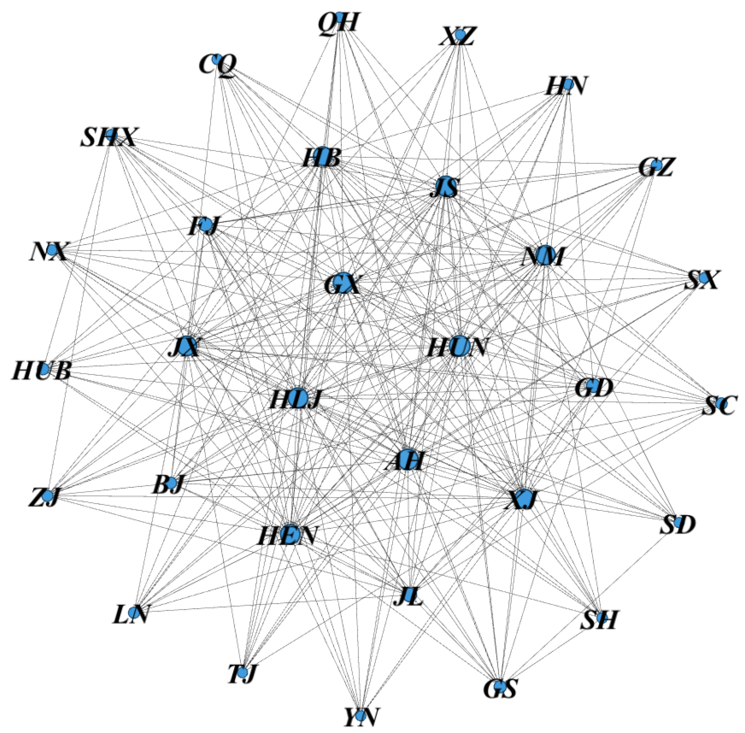
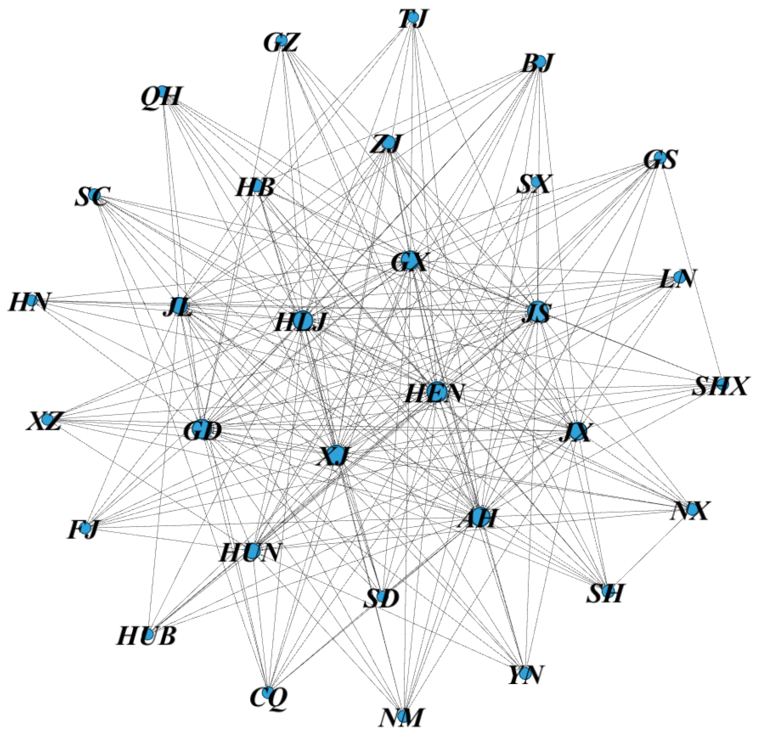
3.2. Analysis of Inter-Provincial Virtual Water Trade Transfer Networksin China

3.2.1. Overall Network Characterization

In order to analyze virtual water transfers in each region of China, this study adopts the social network analysis method to construct a virtual water trade transfer network of 31 provinces in China for visualization and analysis. As shown in Figure 3, Figure 4 and Figure 5, each province is represented as a node in the network, and the size of the node directly reflects the degree of connectivity (node degree) of the province in the network. A larger node indicates that the province engages in more frequent and influential virtual water trade with other provinces. Among them, the nodes in Xinjiang, Heilongjiang, Jiangsu, Guangxi, and Guangdong were more significant in all three years, which indicates that these provinces occupy a central position in the virtual water trade network.

In terms of the overall characteristics of the network, it can be observed in

Table 7. Overall characteristics of the network.

Year	Node	Edge	Network Density	Symmetry	Average Clustering Coefficient	Average Path Length
2012	31	320	0.344	0.331	0.703	1.541
2015	31	330	0.355	0.342	0.646	1.446
2017	31	283	0.304	0.322	0.645	1.686

that the network density and symmetry showed an upward trend from 2012 to 2015. The increase in network density indicates that virtual water trade connections have strengthened, which may be related to the deepening of global economic integration, the construction of a unified national market, and the optimization of water resource management strategies. Meanwhile, the increased symmetry implies an improved balance in virtual water trade relations, and regions are more equal in trade. However, by 2017, both network density and symmetry declined. Declining network density suggests that, in the face of global challenges such as water scarcity and climate change, some regions may have adopted more conservative trade policies and reduced virtual water exports to protect local water security. Among them, China’s Action Plan for the Prevention and Control of Water Pollution (Water Ten), released in April 2015, is a national-level water resource control policy that imposes strict pollution prevention and water conservation requirements on water-intensive industries, including upgraded wastewater discharge standards and regional discharge restriction policies. These industries include the chemical, printing and dyeing, and coal sectors. Implementing this policy has disrupted the original cost-based inter-provincial trade balance. Some provinces have withdrawn from the production chain of high-water-consuming products. This has directly reduced the number of connections of inter-provincial virtual water flows and ultimately led to a decrease in network density. A decrease in symmetry, on the other hand, suggests that the equilibrium of virtual water trade relations has been disrupted, and individual regions have become more prominent in trade. In addition, the yearly decrease in the average clustering coefficient reveals the gradual disintegration of the clique structure in the network, probably due to the diversification of trading partners, the intensification of competition in the market, and the lowering of trade barriers as a result of technological advances. In contrast, the initial decrease followed by an increase in the average pathlength shows a tendency for the efficiency of the network to rise and then fall, which may be related to factors such as the simplification of trade processes, advances in information technology, and the subsequent increase in the number of trade barriers.

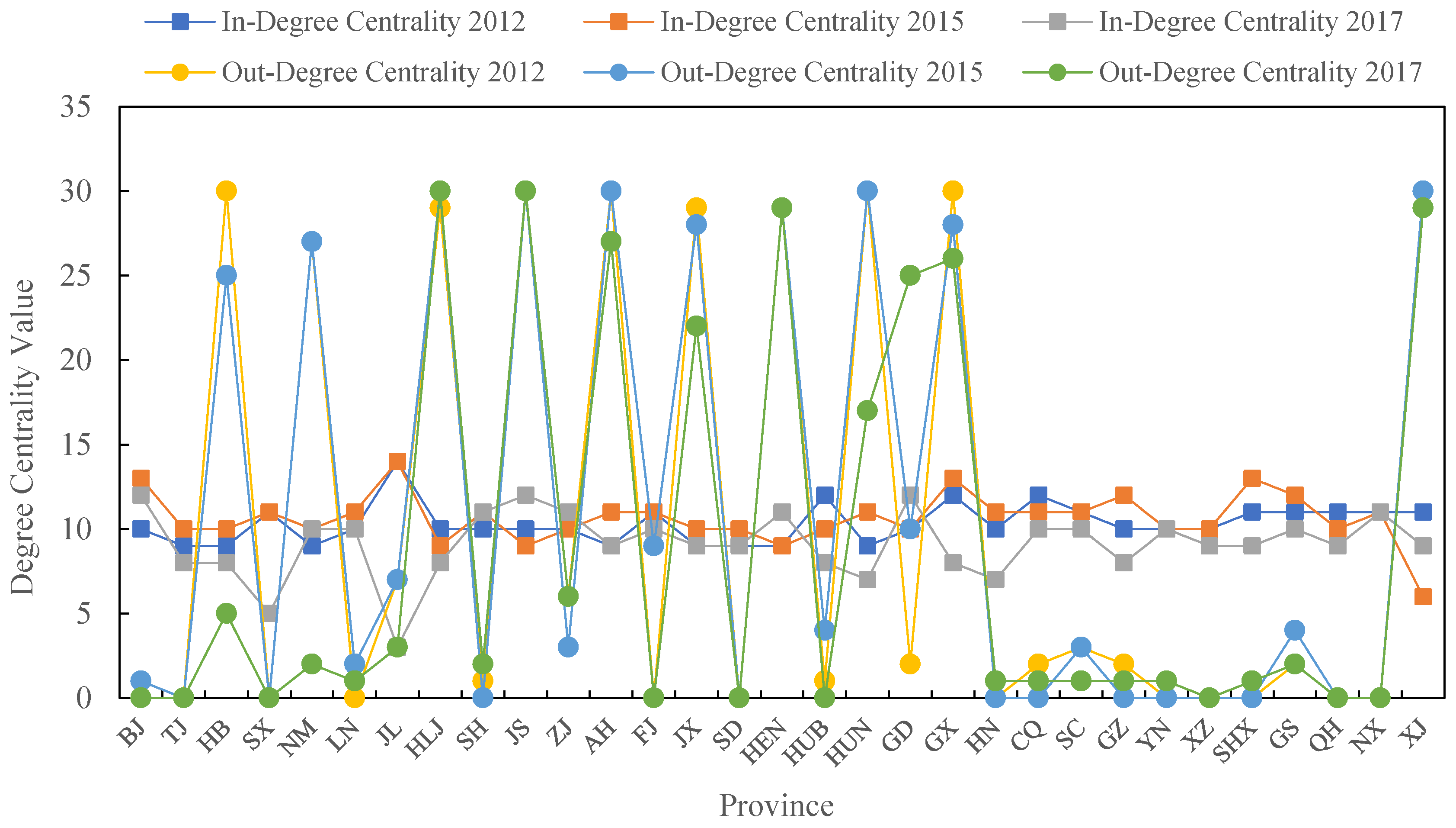
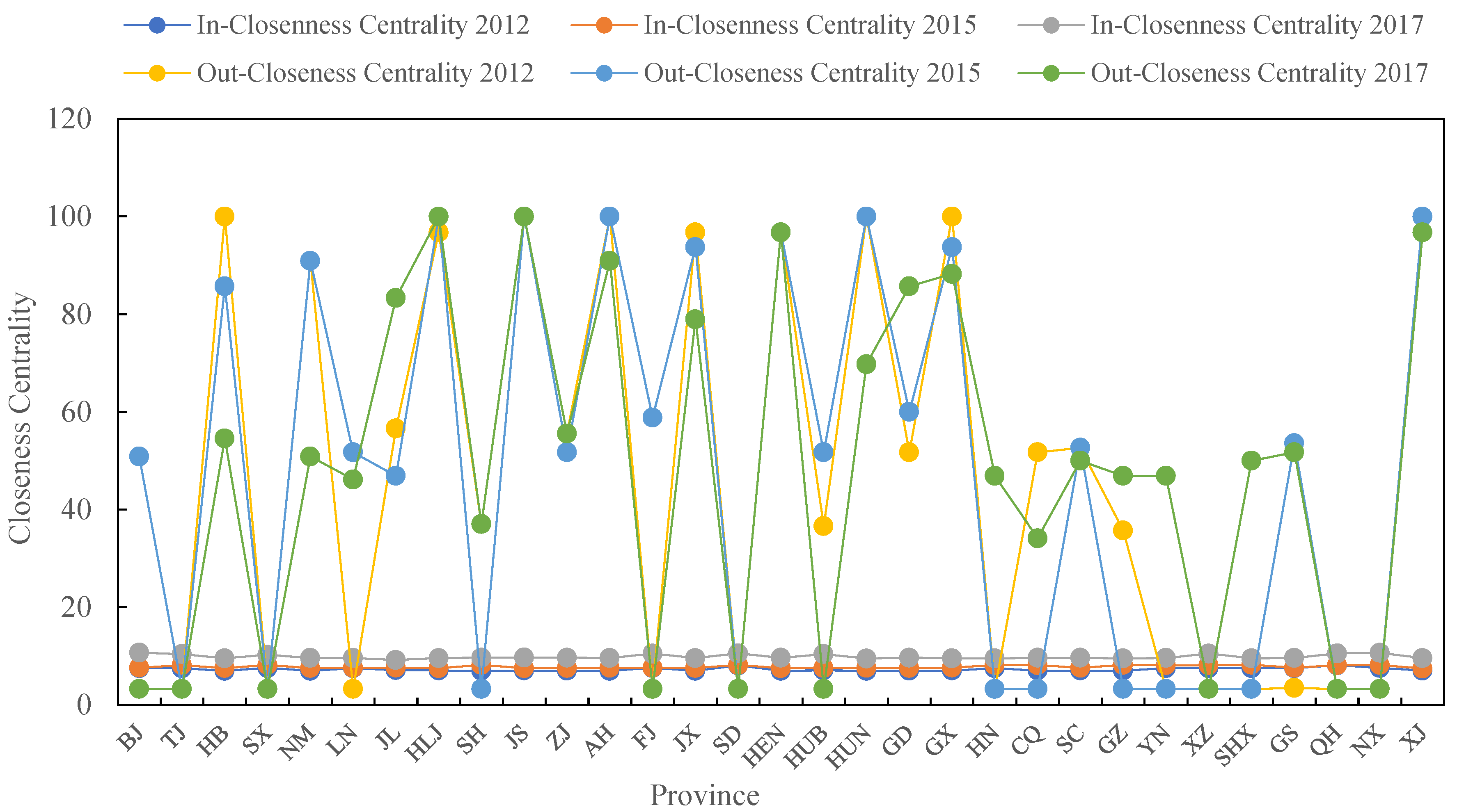
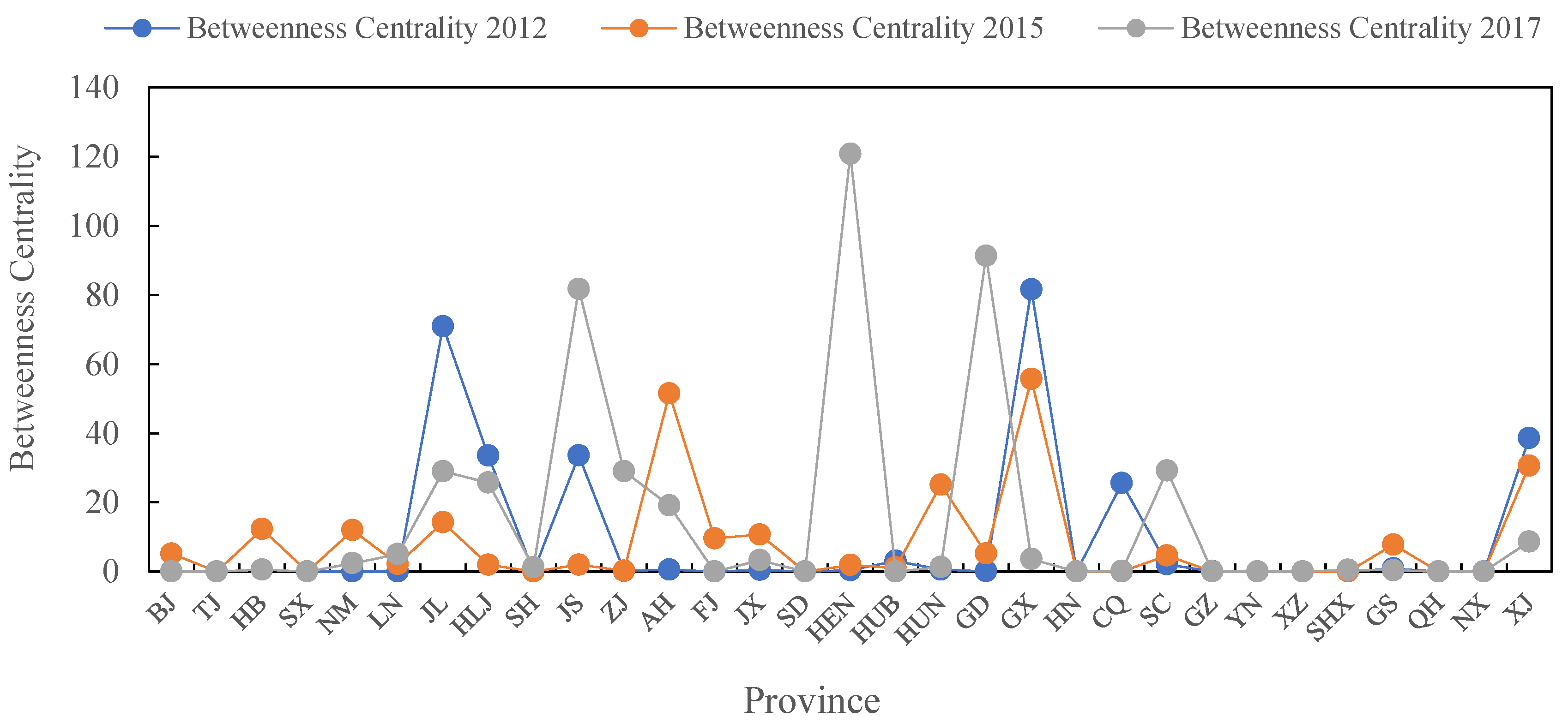
3.2.2. Individual Network Characterization

To gain a deeper understanding of the individual characteristics of the network, this study calculates the degree centrality, proximity centrality, and intermediate centrality in the virtual water trade transfer network of 31 provinces in China (for 2012, 2015, and 2017), and the results are shown in Figure 6, Figure 7 and Figure 8.

In terms of degree centrality, provinces such as Jiangsu, Xinjiang, Heilongjiang, and Guangxi exhibited higher degree centrality with respect to out-degrees during this period, playing the role of water exporters. The number of virtual water export objects in water-intensive provinces such as Hebei and Jiangxi decreased year by year, indicating a gradual weakening of their network centrality. This may be related to the strengthening of the national policy on water resource protection, and these regions have effectively reduced unnecessary virtual water outflow through refined water resource management. The out-degree centrality of municipalities such as Beijing and Tianjin remains zero, reflecting their minimal activity in water outflows, which is closely related to their water scarcity and strict water management policies. Simultaneously, provinces such as Beijing, Zhejiang, Fujian, and Shanghai have high in-degree centrality, indicating that virtual water mainly flows to economically developed regions. These regions have frequent economic activities, high water demand, and stronger economic strength and technology levels, and they are able to utilize virtual water resources more efficiently.

In terms of closeness centrality, Heilongjiang, Jiangsu, Anhui, Xinjiang, and other provinces have high out-degree closeness centrality and strong virtual water resource “radiation” capacity. In contrast, the out-degree closeness centrality of Hunan and Guangxi declined in 2017, probably due to increasing water scarcity and insufficient deployment capacities. At the same time, improvements in water resource management and water infrastructure in other provinces may have weakened the dependence on virtual water resources in Hunan and Guangxi. In contrast, Shanxi, Fujian, Shandong, Qinghai, and Ningxia show a very high in-degree closeness centrality, implying that they have a strong ability to integrate resources in the network. In addition, the provinces of Beijing, Tianjin, Shanghai, Hainan, Chongqing, Tibet, Guizhou, Yunnan, and Shanxi show a significant increase in in-degree closeness centrality over time, thanks to the optimization of water resource management policies and the improvement in water infrastructure, which enhances their attractiveness and integrative power in the network.

In terms of betweenness centrality, the provinces of Guangxi, Jilin, Xinjiang, and Jiangsu played an important intermediary role in the network in 2012 by virtue of their rich resources and convenient transportation networks. In 2015, Anhui significantly increased the influence of their network by improving regional economic cooperation and transportation infrastructure. By 2017, Henan, Guangdong, and Jiangsu provinces had become the core intermediaries in the network by virtue of their economic strength, efficient logistics systems, and strategic locations in the national network. Simultaneously, the betweenness centrality of Sichuan and Zhejiang provinces was relatively low in 2012 and 2015. However, by 2017, through deepened regional cooperation and improved internal transportation and logistics systems, the connectivity and radiation capacity of these provinces within the national network were significantly enhanced, leading to a significant increase in their betweenness centrality.

3.2.3. Analysis of Block Model Results

Between 2012 and 2017, the interactions among the four major economic sectors in China showed remarkable features and changes, and these data profoundly revealed the diversity and complexity of regional economic cooperation, as shown in

Table 8. Spatial correlation relationships in China’s virtual water trade transfer network in 2012.

	Plate I	Plate II	Plate III	Plate IV
Plate I	5	5	0	3
Plate II	3	6	2	2
Plate III	132	30	56	16
Plate IV	34	8	16	2
Number of Section Provinces	17	4	8	2
Number of Spillover Relationships	8	7	178	58
Number of Receiving Relationships	169	43	18	21
Expected Internal Relationship Ratio (%)	53.33	10	23.33	3.33
Actual Internal Relationship Ratio (%)	38.46	46.15	23.93	3.33
Section Type	Bidirectional Spillover Section	Main Beneficiary Section	Net Spillover Section	Broker Section
Section Names	Beijing, Tianjin, Yunnan, Shanxi, Shaanxi, Liaoning, Qinghai, Shandong, Shanghai, Guizhou, Zhejiang, Guangdong, Fujian, Hainan, Gansu, Ningxia, Tibet	Hubei, Sichuan, Chongqing, Jilin	Anhui, Hunan, Henan, Hebei, Inner Mongolia, Heilongjiang, Jiangsu, Jiangxi	Guangxi, Xinjiang

,

Table 9. Spatial correlation relationships in China’s virtual water trade transfer network in 2015.

	Plate I	Plate II	Plate III	Plate IV
Plate I	2	8	0	2
Plate II	20	1	6	4
Plate III	18	38	6	18
Plate IV	56	89	21	41
Number of Section Provinces	8	13	3	7
Number of Spillover Relationships	10	30	74	166
Number of Receiving Relationships	94	135	27	24
Expected Internal Relationship Ratio (%)	23.33	40	6.67	20
Actual Internal Relationship Ratio (%)	16.67	3.23	7.5	19.81
Section Type	Bidirectional Spillover Section	Main Beneficiary Section	Net Spillover Section	Broker Section
Section Names	Beijing, Guizhou, Yunnan, Jilin, Shaanxi, Hainan, Gansu, Chongqing	Tianjin, Shanxi, Zhejiang, Guangdong, Hubei, Qinghai, Sichuan, Ningxia, Shanghai, Liaoning, Tibet, Shandong, Fujian	Guangxi, Hebei, Inner Mongolia	Hunan, Henan, Anhui, Jiangsu, Jiangxi, Heilongjiang, Xinjiang

and

Table 10. Spatial correlation relationships in China’s virtual water trade transfer network in 2017.

	Plate I	Plate II	Plate III	Plate IV
Plate I	7	1	10	0
Plate II	2	2	2	0
Plate III	122	34	49	15
Plate IV	27	0	11	1
Number of Section Provinces	16	5	8	2
Number of Spillover Relationships	11	4	171	23
Number of Receiving Relationships	151	35	23	15
Expected Internal Relationship Ratio (%)	50	13.33	23.33	3.33
Actual Internal Relationship Ratio (%)	38.89	33.33	22.27	2.56
Section Type	Bidirectional Spillover Section	Main Beneficiary Section	Net Spillover Section	Broker Section
Section Names	Beijing, Hubei, Yunnan, Zhejiang, Inner Mongolia, Liaoning, Chongqing, Sichuan, Shanghai, Guizhou, Qinghai, Shaanxi, Fujian, Ningxia, Tibet, Gansu	Shanxi, Hebei, Shandong, Tianjin, Hainan	Guangxi, Henan, Jiangsu, Jilin, Guangdong, Anhui, Xinjiang, Heilongjiang	Jiangxi, Hunan

.

In 2012, Plate I, which covers a large number of eastern and central–western provinces, exhibited strong two-way spillover characteristics, illustrating its central position in regional economic interactions and its dual role inactively exporting resources and extensively absorbing external influences. In contrast, Plate II, despite its limited number of provinces, exhibits strong internal ties and plays more of a beneficiary role, with a significantly higher number of receiving relationships than spillovers and a regional economy strongly influenced by external factors. Plate III, on the other hand, shows significant net spillover effects and is a strong representative of resource-exporting regions. Plate IV, despite having the fewest provinces, plays a key connection role between the plates, exhibiting a balanced pattern of exchanges, and it isa broker plate that promotes regional economic connectivity.

In 2015, despite its low number of provinces, Plate I had frequent exchanges with other plates, and the number of receiving ties was substantially higher than the number of spillovers, reflecting its role as a resource absorber. Its internal ties are slightly lower, but its diverse economic characteristics, including the coexistence of municipalities and western provinces, allow this plate to occupy an important position in the regional economy. Plate II has a large number of provinces covering the east, central, and west regions, but it is characterized by loose internal links and a high dependence on external resource inputs, with significant main beneficiary characteristics. Simultaneously, Plate III has become a net spillover region in the regional economy due to its strong resource-exporting ability. Its provinces are mostly located in the resource-rich north, which provides strong support for regional economic development. Plate IV, on the other hand, continues to play its role as a broker plate, with extensive, balanced exchanges with other plates and stable internal connections. Its provinces cover the central and eastern parts of the country and the border areas, with significant geographic advantages.

In 2017, Plate I, as a large integrated plate, had a high number of both spillover and receiving relationships but a slightly lower proportion of internal connections. This reflects its two-way interaction within the regional economy, some capacity for resource exports, and a broad composition of provinces with diversified economies. Plate IIhas fewer provinces but is located in a key position, with a higher number of receiving relationships than spillovers and a relatively high proportion of internal connections, indicating that it benefits from external resource inputs and is highly dependent on economic development. Plate III has further increased its resource-exporting capacity and has become a stable net spillover region in the national economy. Most of its provinces are either large resource provinces or economically powerful provinces, providing significant momentum for regional economic development. Plate IV, on the other hand, with its balanced number of spillovers and receiving relationships, plays an indispensable role as a bridge in regional economic cooperation despite its weak internal connections.

Analyzing the density and image matrices of the spatial associations of the virtual water trade transfer network in China for the 2012, 2015, and 2017 periods, we can observe that the associations between the plates show significant changes between years, as shown in

Table 11. Density and image matrices of spatial correlation blocks in China’s virtual water trade transfer network in 2012.

Tectonic Plate	Density Matrix				Image Matrix
	Plate I	Plate II	Plate III	Plate IV	Plate I	Plate II	Plate III	Plate IV
Plate I	0.018	0.074	0.000	0.088	0	0	0	0
Plate II	0.044	0.500	0.063	0.250	0	1	0	0
Plate III	0.971	0.938	1.000	1.000	1	1	1	1
Plate IV	1.000	1.000	1.000	1.000	1	1	1	1

,

Table 12. Density and image matrices of spatial correlation blocks in China’s virtual water trade transfer network in 2015.

Tectonic Plate	Density Matrix				Image Matrix
	Plate I	Plate II	Plate III	Plate IV	Plate I	Plate II	Plate III	Plate IV
Plate I	0.036	0.077	0.000	0.036	0	0	0	0
Plate II	0.192	0.006	0.154	0.044	0	0	0	0
Plate III	0.750	0.974	1.000	0.857	1	1	1	1
Plate IV	1.000	0.978	1.000	0.976	1	1	1	1

and

Table 13. Density and image matrices of spatial correlation blocks in China’s virtual water trade transfer network in 2017.

Tectonic Plate	Density Matrix				Image Matrix
	Plate I	Plate II	Plate III	Plate IV	Plate I	Plate II	Plate III	Plate IV
Plate I	0.029	0.013	0.078	0.000	0	0	0	0
Plate II	0.025	0.100	0.050	0.000	0	0	0	0
Plate III	0.953	0.850	0.875	0.938	1	1	1	1
Plate IV	0.844	0.000	0.688	0.500	1	0	1	1

. In 2012, the density matrix values of both Plate III and Plate IV reached 1.000, indicating that the virtual water trade connections within these two plates and among other plates are extremely strong. This may be related to the fact that most provinces within Plate III and Plate IV are large agricultural provinces with high water demands, and they are geographically close to each other, which facilitates water trade. In contrast, Plate I and Plate II are not as geographically close to one another, reflecting the relative isolation of these plates in the virtual water trade network. Entering 2015, Plate III still maintained a high degree of correlation, while Plate IV’s correlation with other plates weakened, especially its correlation with Plate I, which dropped significantly to 0.036. This change may stem from the fact that provinces in Plate IV, such as Xinjiang, have weakened their trade linkages with other regions due to their remoteness and the high cost of trading water resources. On the other hand, the correlation within Plate II plummeted to 0.006, probably because provinces within the plate, such as Jilin and Hubei, have significant differences in their economic development levels and water resource distributions, resulting in relatively weak internal trade connections. In particular, the correlation between Plate II and Plates III and IV increased, reflecting the positive role played by national policies in promoting regional water resource cooperation. By 2017, the connections of Plate III were high, but the connections observed in Plate IV continued to decline, particularly with respect to Plate II and its own internal connections, which dropped to a lower level. This may be attributed to industrial restructuring in provinces such as Jiangxi and Hunan within Plate IV, which has reduced their demand for water resources and thus weakened their trade links with other plates. Meanwhile, the linkage between Plate I and Plate III increased to 0.078. This can be attributed to provinces, such as Shaanxi and Chongqing in Plate I, strengthening their water resource management and improving their utilization efficiency, which in turn led to greater dependence on external water resources. In addition, internal correlations within Plate II also increased, but they remained low overall, indicating that the relative isolation of this plate in the virtual water trade network did not fundamentally change.

3.2.4. Network Structural Resilience Analysis

In this study, the Gephi software 0.10.1 was used to calculate the network structure’s resilience-related indexes, as shown in

Table 14. Characteristics of network structural resilience.

Year	K1	K2	K3	K4	K	T
2012	0.703	1.541	−0.838	−0.225	0.827	T3
2015	0.646	1.446	−0.600	−0.268	0.740	T3
2017	0.645	1.686	−0.800	−0.303	0.857	T3

Note: K₁ denotes agglomeration, K₂ denotes transmissibility, K₃ denotes hierarchy, K₄ denotes matching, and K denotes the network structural resilience index. T denotes the type of network structural resilience, T₁ denotes a stochastic network, T₂ denotes a homoscedastic core–edge network, and T₃ denotes a resilience network.

.

• Network Agglomeration and Transmission

During 2012 and 2015, agglomeration decreased from 0.703 to 0.646, indicating weaker connections between nodes and a sparser local network structure. This is likely due to the weakening of certain existing relationships and the delayed formation of new ones as the network evolved. Transmissibility decreased from 1.541 to 1.446, indicating a reduction in the efficiency of transmission between nodes and a decline in overall connectivity. By 2017, the agglomeration indexes remained relatively stable, while the transmissibility index appeared to increase significantly. This suggests that the information transmission efficiency increased significantly while the network structure was stable, likely resulting from network optimization measures and the general application of new technologies.

2.

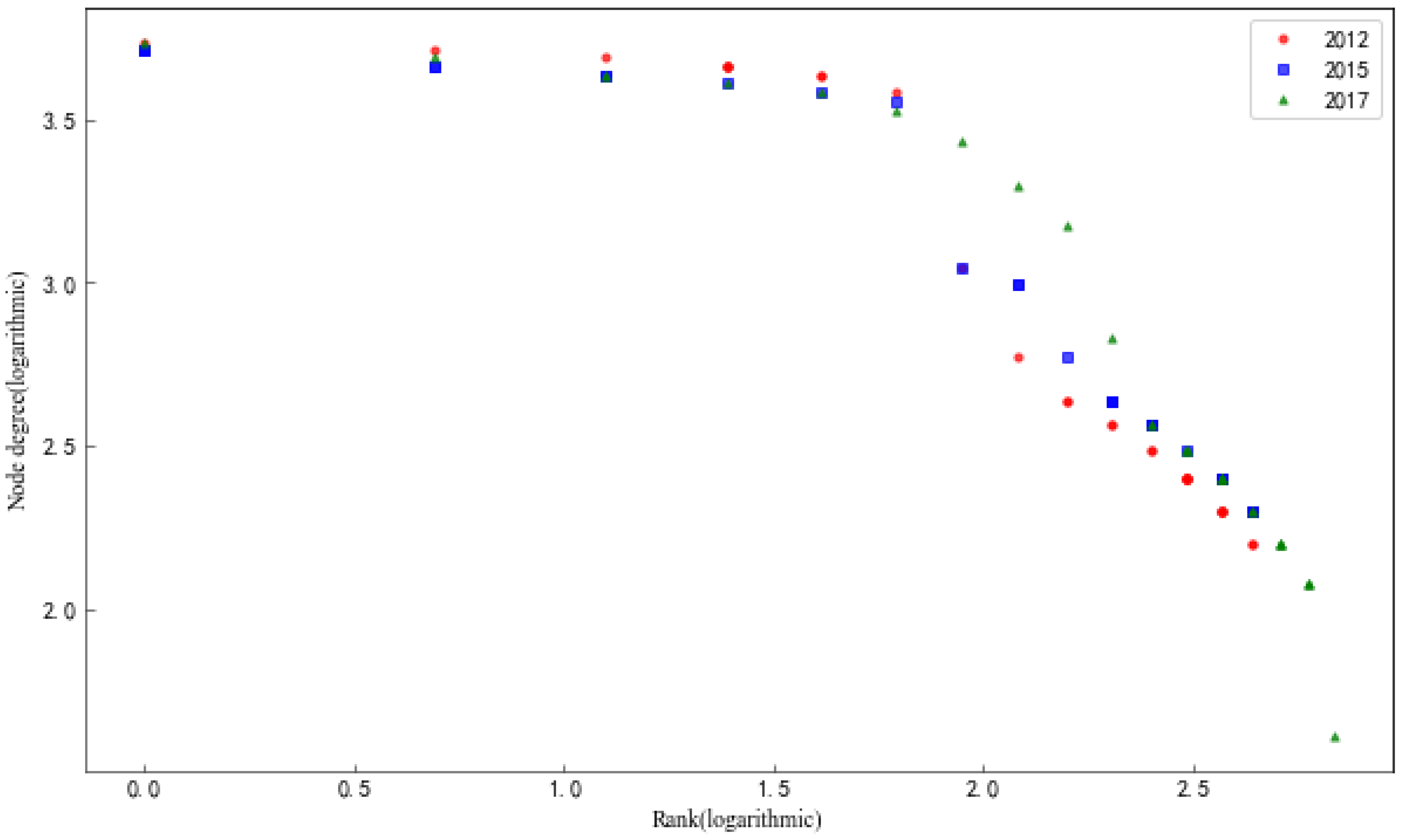
Network Hierarchy—Degree Distribution

According to Equation (16), we measured the hierarchical nature of the virtual water trade transfer network in 2012, 2015, and 2017, and the results of the degree distribution are shown in Figure 9. The hierarchical nature of the network was significant in 2012, and the slope of the curve was 0.84, indicating the existence of a clear core–edge structure, with a few core provinces occupying an important position in virtual water trade by virtue of their high connectivity, while most edge and marginal provinces had relatively weak connectivity. By 2015, the slope declined to 0.60, reflecting a weakening of the network hierarchy and a reduction in the difference in connectivity. This suggests a more balanced distribution and an increase in the number of provinces involved in virtual water trade transfers. This may be attributed to factors such as policy adjustments or technological advances that have facilitated the widespread dissemination and balanced development of the virtual water trade. The slope of the curve rebounded to 0.80 in 2017, indicating a restoration of the hierarchical structure and a renewed increase in imbalance within the degree distribution. However, compared to 2012, the curve was smoother that year, indicating that, under the combined influence of policy guidance and market mechanisms, the key roles of some provinces in virtual water trade were reinforced, while the overall network structure became more stable.

3.

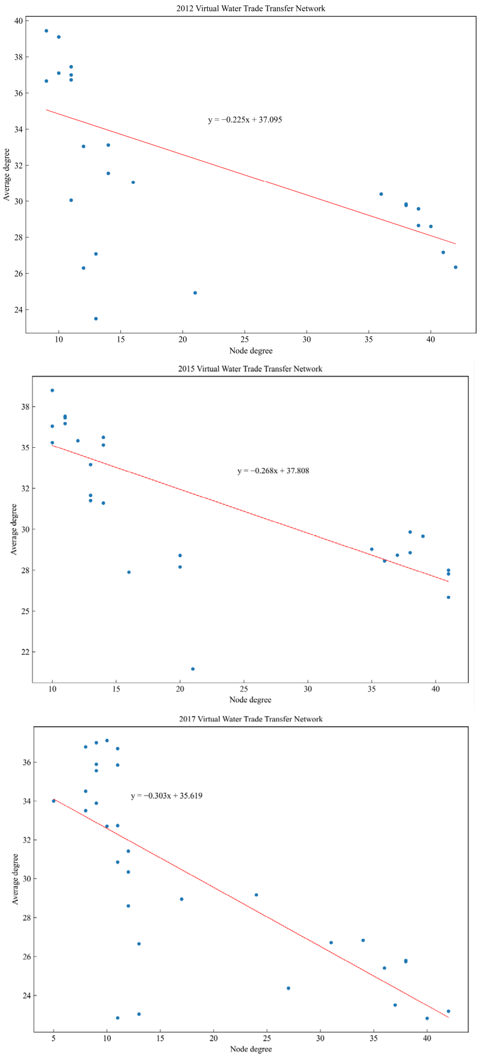
Network Matchability—Degree Correlation

In order to gain insight into the matching between the nodes of the network, a degree correlation diagram is drawn based on Equations (17) and (18), as shown in Figure 10 and Figure A1.

The degree correlation coefficient b is an important indicator for measuring the size of changes in the degree correlation of nodes in a network. In the three 2012, 2015, and 2017 time points, the degree correlation coefficient b is less than 0, indicating that China’s virtual water trade transfer network is characterized by heterogeneity, i.e., provinces with a higher number of connections are more inclined to establish trade links with provinces with a lower number of connections. Meanwhile, the absolute value of the degree connection coefficient increased each year over this three-year period, which indicates that the matching intensity of the virtual water trade transfer network increased year by year. That is, trade links between high-connectivity provinces and low-connectivity provinces became stronger and more frequent over time, and this heterogeneous matching characteristic became increasingly significant in the network. Highly connected provinces have more resources and market advantages, while low-connectivity provinces obtain the required virtual water resources by establishing trade links with these provinces. This complementary resource mechanism and benefit sharing became more effective and stable as the matching strength of the network increased.

4.

Network structural resilience index and type determination

According to the data in Table 14, the network structural resilience index decreased from 0.827 in 2012 to 0.740 in 2015, which may be related to external challenges or internal structural adjustments faced by some provinces. However, in 2017, the index rebounded to 0.857, showing that the network was effectively enhanced with respect to resilience by means of optimal resource allocation, enhanced node connectivity, or the adoption of new management mechanisms. In terms of the type of network structural resilience, during this period, the virtual water trade transfer networks acrossChina’s31 provinces were all classified as resilient networks. This implies that the networks were more structurally resilient and that innovative behaviors were able to smoothly diffuse from peripheral members to core members. This characteristic helps promote resource flow and information sharing within a network, thus enhancing the stability and adaptive capacity of the entire network.

3.3. Analysisof Actors Influencing Inter-Provincial Virtual Water Trade Networksin China

3.3.1. Analysis of ERGM Results

In this study, the annual average virtual water trade in 2012, 2015, and 2017 is used as the benchmark sample for the ERGM estimation of virtual water trade transfer networks, and the results are shown in

Table 15. Estimation results of the exponential random graph model.

Variable	Model1	Model2	Model3	Model4
Edges	−0.64883 ***	−6.54569 ***	−2.12634 ***	−4.13970 ***
	(0.07280)	(1.61944)	(0.24242)	(1.17647)
Mutual		4.92591 ***		4.43934 ***
		(0.48709)		(0.77318)
Twopath		−0.19600 ***		−0.14295 ***
		(0.02704)		(0.03454)
Balance		−0.50945 ***		−0.50399 ***
		(0.05690)		(0.08453)
Gwesp.OTP.fixed.0.2		6.16043 ***		3.49659 ***
		(1.36829)		(0.97630)
Sender(gdp)			−0.00004 ***	0.00000
			(0.00001)	(0.00001)
Sender(popu)			−0.00047 ***	0.00003
			(0.00006)	(0.00008)
Sender(pwater)			0.00010 **	0.00011 *
			(0.00004)	(0.00004)
Receiver (gdp)		−	0.00000	−0.00002 *
			(0.00001)	(0.00001)
Receiver(popu)			−0.00000	0.00031 ***
			(0.00005)	(0.00006)
Receiver(pwater)			0.00012 **	0.00009 *
			(0.00004)	(0.00004)
Absdiff(gdp)			0.00001	0.00002 *
			(0.00001)	(0.00001)
Absdiff(popu)			−0.00008	−0.00019 ***
			(0.00005)	(0.00005)
Absdiff(pwater)			−0.00012 **	−0.00012 *
			(0.00004)	(0.00005)
Edgecov(spadis)		0.39487		0.33584
		(0.32151)		(0.32276)
Edgecov(D[0,500])		0.05104		−0.87246
		(0.35631)		(0.46656)
Edgecov(D[500,1000])		−0.41625		−1.40761 ***
		(0.23908)		(0.35269)
Edgecov(D[1000,1500])		−0.41320 *		−1.18609 ***
		(0.19906)		(0.29878)
Edgecov(D[1500,2000])		−0.69705 *		−1.61553 ***
		(0.30585)		(0.35041)
AIC	−92.09426	−282.96777	−223.26979	−369.92227
BIC	−87.25907	−234.61592	−174.91794	−278.05376

Note: *, **, and *** represent significance at the 5%, 1%, and 0.1% levels, respectively.

. Among them, Model 1 is a benchmark model containing only node attribute effects, Model 2 is a composite mechanism model containing endogenous structural variables and exogenous network covariates, Model3 is an attribute model containing only actor attribute variables, and Model 4 isa composite test model containing endogenous structural, actor attribute, and exogenous network covariates.

In Model 1, the edges’ estimated parameters are all presented with negative values, a result that suggests that the network structure of the virtual water trade transfer relationship is not randomly constructed.

In Model 2, the arc, reciprocity, connectivity, stability, and agglomeration coefficients are all significant at the 0.1% level, confirming the existence of a real and stable correlation between the endogenous structural variables and the model. Specifically, the coefficient of reciprocity is significantly positive, revealing a high degree of interdependence with respect to virtual water trade transfers among provinces. The connectivity coefficient is significantly negative, indicating that the number of active provinces with both sending and receiving capacities is relatively scarce. The stability indicator is significantly negative, reflecting the asymmetry, instability, or unbalanced network structure of the virtual water trade relationship among provinces. In addition, the geographic proximity network, which is an exogenous covariate, is not significant at the distance intervals [0,500] and [500,1000], while the distance intervals [1000,1500] and [1500,2000] are significantly negative at the 5% level, indicating that the trade relations between provinces at closer geographical distances experience interference with non-geographic factors and that longer distances are susceptible to factors such as trade costs and logistics constraints. In contrast, the spatial distance network is insignificant with a positive coefficient, probably because its effect is masked by other, more critical, structural variables.

In Model 3, in terms of the sending effect, both gdp and population size are significantly negative at the 0.1% level, probably because the economic development and population growth in the relevant regions result in an increase in the demand for local water resources, which reduces the amount of virtual water available for export. The amount of water resources per capita is significantly positive at the 1% level, suggesting that the imbalance in the distribution of water resources plays a key role in virtual water trade. The richer a region’s water resources per capita, the relatively lower its costs of agricultural production and water utilization, and therefore the more likely it is to be a virtual water exporter. Second, in terms of the reception effect, although the gdp and population size do not reach a significant level, a positive gdp coefficient implies that economically developed regions have a stronger demand for virtual water imports, and a negative popu coefficient implies that the direct demand for virtual water in densely populated regions is mitigated by other factors (such as water resource management policies, water conservation technologies, etc.). In particular, water per capita is significantly positive at the 1% level, further confirming the strong link between the two. In addition, the analysis of dissimilarity (Absdiff) reveals that water resources per capita are significantly negative at the 1% level, indicating that when the difference in water resources per capita between the two regions is smaller, the likelihood of forming a trade transfer relationship between them is higher. In other words, there is a convergence effect between different provinces in terms of per capita water resource ownership, possibly because similar water resource endowment promotes mutual water resource demand and supply in trade.

In Model 4, the arc, reciprocity, connectivity, stability, and agglomeration coefficients continue to be highly significant. On the sending effect, the gdp and population size coefficients are positive, but neither reaches the significance level, implying that the influence of traditional economic factors is overshadowed by other, more critical water-related factors in determining virtual water exports. However, the amount of water per capita is positive at the 5% significance level, emphasizing the advantage of water-rich regions as virtual water exporters. In the reception effect, gdp is negative at the 5% significance level, which may be related to the more efficient use of water resources in economically developed regions and their natively lower demand for virtual water imports. In contrast, population size is positive at the 0.1% significance level, indicating that the demand for virtual water is more urgent in densely populated areas. Water per capita (p water) is positive at the 5% significance level, further confirming the important role of water scarcity in driving virtual water imports. Heteroscedasticity analysis, on the other hand, reveals the impact of attribute differences between provinces on virtual water trade. Differences in gdp are positive at the 5% significance level, indicating that trade relationships are more likely to be formed between provinces with similar levels of economic development. The difference in population size is negative at the 0.1% significance level, indicating that there are fewer trade relationships between provinces with similar population sizes, which may be related to differences in population distribution, consumption habits, and other factors. The difference in water resources per capita is negative at the 5% significance level, emphasizing that trade relations are more likely to be established between provinces with similar water resource endowments. In addition, among the exogenous covariates, the spatial proximity network is insignificant and has a positive coefficient, suggesting that spatial proximity has a relatively weak effect on virtual water trade. The geographic proximity network is insignificant and has a negative coefficient in the distance interval [0,500]. In contrast, it is negative at the0.1% significance level in the distance intervals [500,1000], [1000,1500], and [1500,2000], suggesting that the cost of long-distance trade, logistics, and other factors limits the formation of trade relationships.

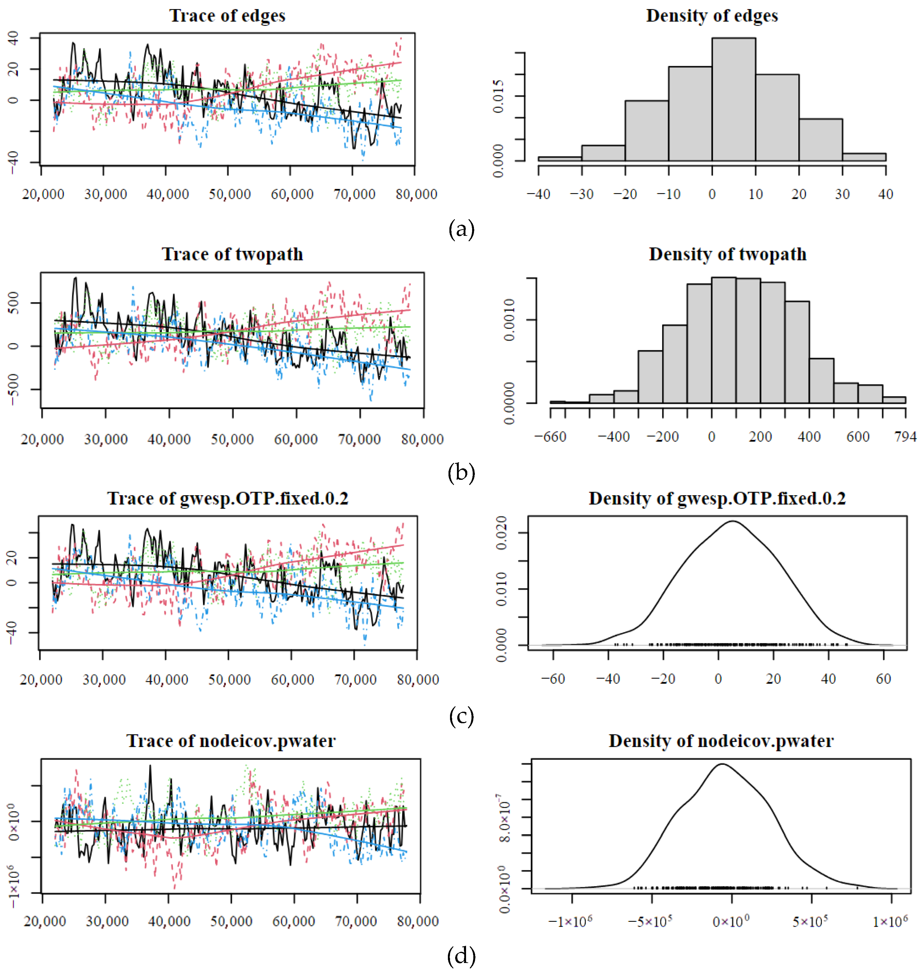
3.3.2. Model Diagnostics

Validation was carried out using the Markov chain Monte Carlo (MCMC) method. Moreover, using the composite test model described in Table 15 as an example, we analyzed the actual network in comparison with the simulated network. Figure 11 depicts the performance of the statistics of the exponential random graph model during the composite model’s final iteration phase. Specifically, the left figure plots the changes in the MCMC chain for each statistic in the model separately using time series, visualizing the dynamic fluctuation in the statistic with the iterative process. The right figure further shows the distribution pattern of these MCMC chains corresponding to the statistics. After model diagnosis, we find that the graphs of all statistics basically show the characteristics of random fluctuation centered on 0, which indicates that the model has good stability. In short, the composite model is confirmed to be stable under the MCMC test.

3.3.3. Model Fitting

The goodness-of-fit test is the core aspect of measuring the quality of model fit, and in exponential random graph models, fit is assessed by comparing the statistical properties of the simulated network with the actual network. Specifically, the magnitude of the values of AIC (Akaike Information Criterion) and BIC (Bayesian Information Criterion) is an important measure of the goodness-of-fit of a model, with smaller values indicating a better fit. The results in the comparison table show that Model 4 had the lowest AIC and BIC values among the mean models in 2012, 2015, and 2017. In addition, we can further judge the model’s fitting effect by the GOF (goodness-of-fit) test results. The black solid line represents real network parameters; the box-and-line plot with a gray solid line indicates the range of simulated network sizes within the 95% confidence interval. By observing the box range of the box plot and the proximity of the black solid line to the gray solid line, we can judge the fitting effect of ERGM to the real network. According to the GOF test results, we find that the simulated network is able to fit the structural features of the real network better on the whole, but there still exists a certain difference between the simulated network and the real network in terms of the incidence and edge-sharing partner features.

4. Conclusions and Recommendations

4.1. Conclusions

This study adopted China’s multi-regional input–output tables and water resource use data from2012, 2015, and 2017 to decompose and account for the volume of virtual water trade from the perspective of value-added trade. We constructed a virtual water trade transfer network for each province in China based on the results of the calculations, and we analyzed network characteristics and network resilience accordingly, ultimately using the exponential random graph model (ERGM) to explore the impact of virtual water trade factors. The main conclusions are as follows:

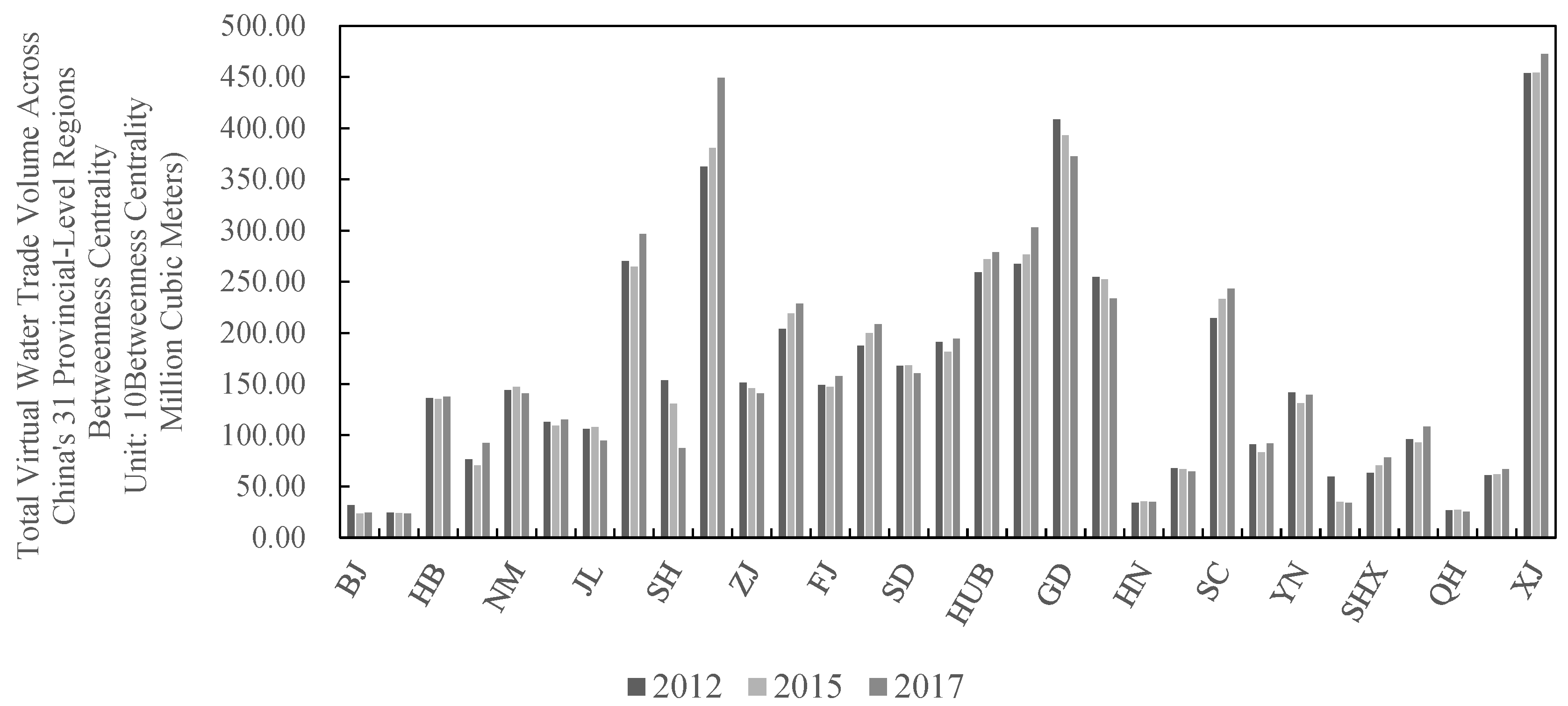
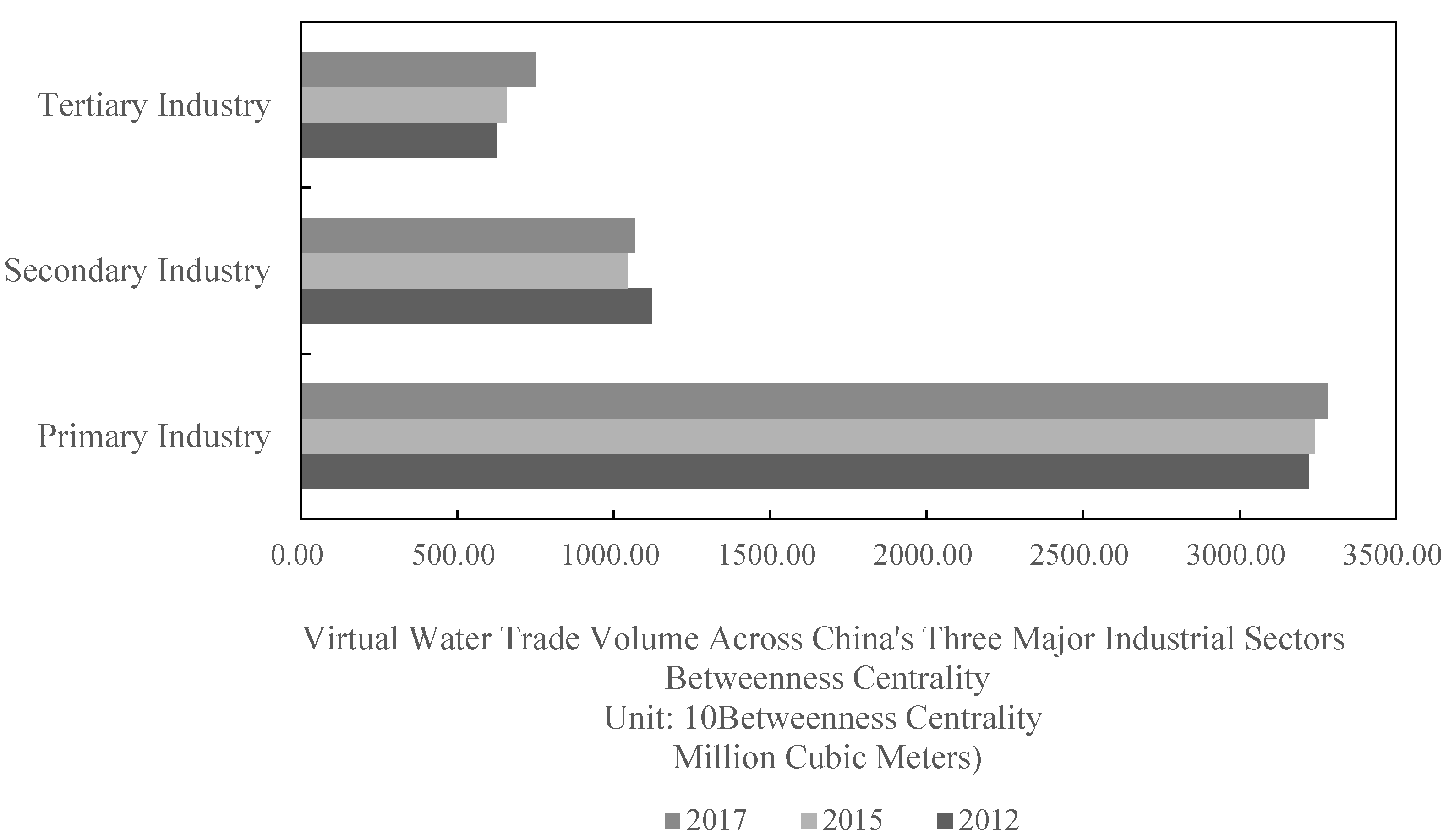
• The total volume of virtual water trade in China’s 31 provinces has stabilized at 494.1–509.9 billion cubic meters. Xinjiang is in the first place due to huge agricultural demand, developed provinces such as Jiangsu and Guangdong are strong, while remote areas such as Shaanxi and Gansu, and water-scarce but high-demand areas such as Beijing and Tianjin have lower trade volumes. The primary sector occupies a central position in the virtual water trade, with the secondary sector declining and then rising, and the tertiary sector decreasing year by year. Water flows are mainly driven by simple value chains, followed by traditional value chains, with small contributions from complex value chains.
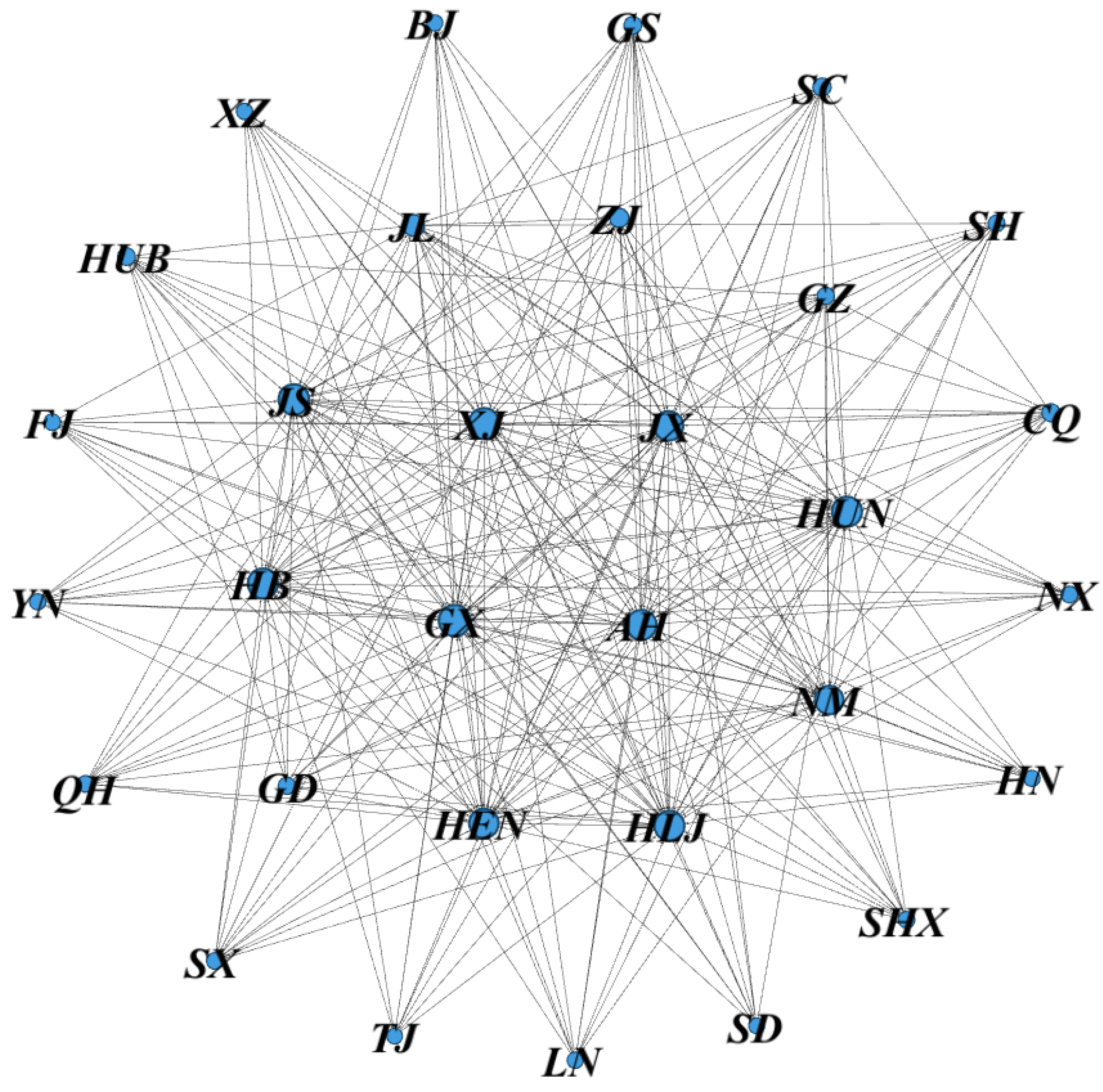
• Social network analysis shows that Xinjiang, Heilongjiang, Jiangsu, Guangxi, and Guangdong are at the core of the virtual water trade network. Network density and symmetry increased in 2012–2015, and slightly decreased in 2017; network efficiency first rises and then falls, and the average clustering coefficient decreases. Jiangsu, Xinjiang, and Heilongjiang continuously export virtual water, and Beijing and Zhejiang are the main receivers. Heilongjiang and Jiangsu have strong radiation capacity; Shanxi and Fujian have strong integration capacity; Guangxi, Jiangsu, Henan, and Guangdong play an intermediary role. Sichuan and Zhejiang have improved their connectivity and radiation capacity through regional cooperation and logistics optimization. The four major economic sectors interact differently: sector 1 has frequent two-way interaction; sector 2 receives significantly; sector 3 has an outstanding net spillover; and sector 4 is the key broker.
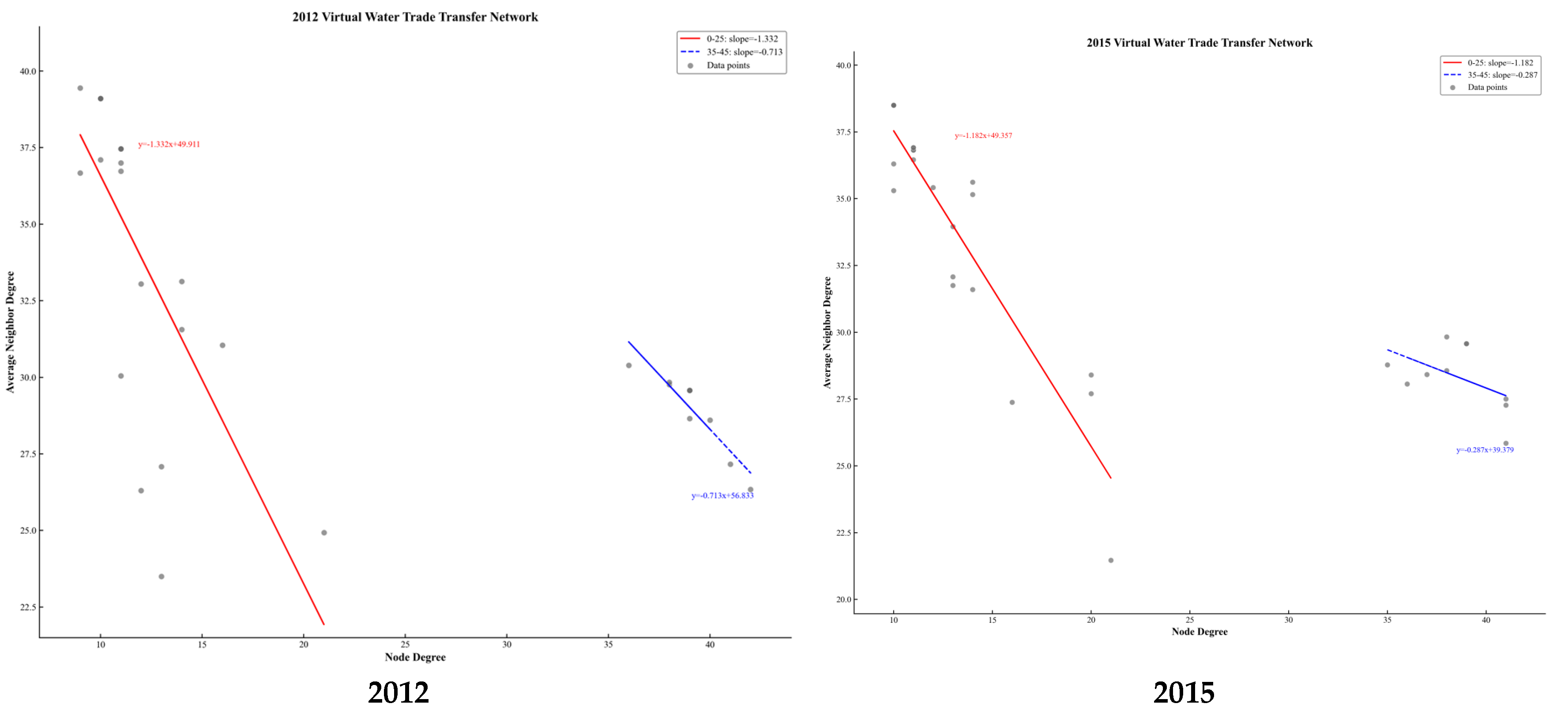
• The structure of the virtual water trade transfer network changes significantly and improves its effectiveness: At the initial stage, the network agglomeration and transferability decrease, presenting a core-edge structure. Then the hierarchical nature of the network is weakened, the degree of connectivity is balanced, and the links between nodes are weakened, resulting in a decrease in connectivity. By 2017, the network hierarchy is restored, the structure is stabilized, and the information transmission efficiency is greatly improved. The degree correlation coefficient continues to be negative and the absolute value increases, indicating that the network heterogeneity characteristics are enhanced. The network structural resilience index rebounded significantly in 2017 after declining in 2015, indicating that the network enhanced its resilience through means such as resource optimization and allocation. During these three years, the network has always been a resilient network with strong structural toughness, which promotes resource flow and information sharing within the network and enhances network stability and adaptability.
• ERGM results show that endogenous structural variables such as arc, reciprocity, connectivity, stability, and agglomeration are highly significant in the annual average virtual water trade transfer network model in 2012, 2015, and 2017. In the sending effect, water resources per capita are significantly positive (water-rich regions are more likely to become virtual water exporters); in the receiving effect, economic development level is significantly negative, population size, and water resources per capita are significantly positive (densely populated and water-scarce regions have a strong demand for virtual water). Heteroscedasticity analysis suggests that similarity in economic development level, population size, and water resource endowment among provinces facilitates virtual water trade. In addition, among the exogenous covariates, the spatial distance network has a weak effect on virtual water trade, and the geographic proximity network is significantly negative in the long-distance interval.

4.2. Recommendations

• Optimizing the layout of the virtual water trade and promoting regional water balance

(1) Regional Differentiated Support: We recommend implementing industrial upgrades in large virtual water-exporting provinces such as Xinjiang and Heilongjiang, and the application of water-saving irrigation(e.g., investment in drip irrigation reduces virtual water runoff), agricultural mechanization, and other technologies should be promoted to improve the efficiency of water resource utilization. Guidance should be provided to developed regions such as Jiangsu and Guangdong in order to reduce water resource consumption through industrial structural adjustment (such as restricting the expansion of high-water-consuming industries) and water-saving technological transformation (such as industrial recycling systems).At the same time, they should be encouraged to safeguard economic water demand through cross-regional cooperation (such as joint construction of water resource allocation projects with remote areas such as Shaanxi and Gansu).

(2) Infrastructure and Policy Synergies: For remote areas such as Shaanxi and Gansu, accelerating the construction of water conservancy infrastructure (e.g., the South-to-North Water Diversion Project) and utilizing the intermediary sector (Sector 4) can facilitate inter-basin water transfers and enhance water resource development capacity. Moreover, a nationwide virtual water trade information platform should be established to share trade data in real time and promote inter-regional water resource cooperation.

(3) Regional Adjustment of High-Water-Consuming Industries: Based on the characteristics of virtual water trade networks, the transfer of high water-consuming industries (such as textile and paper) to areas with abundant water resources and large environmental capacity (such as Xinjiang and Heilongjiang) should be promoted. Simultaneously, the adoption of water-conserving technologies should be guided via policy incentives (such as tax incentives and subsidies).

2.

Strengthening the virtual water trade network and enhancing its effectiveness

(1) Leading Role of Core Nodes: We recommend strengthening the trade hub function of core nodes, such as Xinjiang, Heilongjiang, Jiangsu, etc., and promoting their trade cooperation with inland provinces through policy guidance (such as setting up virtual water trade demonstration zones) and market mechanisms (such as water resource trading platforms). Water resource management should also be strengthened (such as popularizing rainwater harvesting and the reuse of water) in receiving provinces such as Beijing and Zhejiang to minimize wastage.

(2) Optimization of the Function of Intermediary Nodes: Guangxi, Henan, Guangdong, and other provinces are encouraged fully use their geographical advantages, build regional water resources allocation centers, strengthen trade links with upstream and downstream provinces, and promote the rational allocation of water resources through inter-regional cooperation (such as linking the South-to-North Water Diversion Project with local water transfer projects).

(3) Synergy Among the Four Major Economic Sectors: Two-way interactions between Sector 1 (such as the Yangtze River Delta and Pearl River Delta) and Sector 3 (such as the Chengdu–Chongqing region) should be promoted. Resource complementarity between Sector 2 (such as Beijing–Tianjin–Hebei) and Sector 4 (such as Central Plains Urban Agglomeration) should be supported. Inter-sectoral water sharing should be implemented through policy coordination (such as trans-regional water resource compensation mechanisms).

3.

Promoting the optimization of the structure of virtual water trade networks and enhancing their resilience

(1) Network Structure Monitoring and Early Risk Warning: A dynamic monitoring system should be established for the virtual water trade network. The real-time characteristics of the network should be assessed, such as hierarchy and heterogeneity, and contingency plans for high-risk nodes should be formulated (such as provinces that are dependent on a single trading partner).

(2) Cooperation Between High-Connectivity and Low-Connectivity Provinces: The establishment of long-term trade relations between high-connectivity provinces (such as Jiangsu and Guangdong) and low-connectivity provinces (such as Tibet and Qinghai) should be promoted to achieve resource complementarity through technology transfer (such as water-saving irrigation technology) and financial support (such as a water resource protection fund).

(3) Inter-regional Water Resource Allocation Mechanism: In view of the obstacles to long-distance trade caused by geographical proximity, coordination at the national level should be strengthened to promote the interconnection of the eastern and central routes of the South-to-North Water Diversion Scheme and local water transfer projects in order to build a nationwide water resource allocation network.

4.

Optimizing virtual water trade networks and strengthening regional cooperation and resource allocation strategies

(1) Network Construction and Optimization: Based on the results of the ERGM estimation, policies should focus on the reciprocity (such as the establishment of cross-regional water sharing alliances), connectivity (such as improvements in transportation and logistics systems or addressing long-distance trade barriers by subsidizing inter-provincial agro-logistics), and stability (such as signing long-term trade agreements) of virtual water trade.

(2) Resource Endowment-Driven Cooperation: Water resource-rich regions (such as Xinjiang and Heilongjiang) and water-resource-poor and densely populated regions (such as Beijing–Tianjin–Hebei and the Yangtze River Delta) should be encouraged to realize resource complementarity through virtual water trade (such as the export of agricultural products from Xinjiang to Beijing–Tianjin–Hebei).Simultaneously, deeper exchanges of experience and cooperation should be promoted among provinces, especially with respect to water resource management, water conservation technology, ecological protection, and cross-regional synergistic governance.

(3) Policy Synergies and Guarantees: Laws and regulations on inter-regional water resource allocation should be formulated, and the rights and responsibilities of all parties should be clarified. A water resource trading market can be set up to allow transfers of water resource utilization rights between different regions, and international cooperation (such as establishing a cross-border water resource protection mechanism with Central Asian countries) should be encouraged and strengthened to ensure the security of national water resources.

4.3. Limitations

The study also has some limitations, mainly in the following three dimensions: at the data level, it is difficult to completely track the dynamic evolution of the virtual water trade network after 2017 due to the lag in updating China’s multi-region input-output tables; at the scope level, the framework focusing on the 31 provinces in China fails to incorporate the potential impacts of the international virtual water trade on the domestic landscape, and lacks a correlation analysis with the policies of the new development pattern, such as the “double cycle”. In addition, in the face of dynamic factors such as public health emergencies, geopolitical conflicts, and national industrial policy adjustments, the study fails to systematically assess their impact on short-term fluctuations and long-term trends in trade. Future research needs to integrate time-sensitive data, international factors, and policy dynamics in order to reveal the complex features of virtual water trade more comprehensively.

References

1. Allan, J.A. ‘Virtual Water’: A Long Term Solution for Water Short Middle Eastern Economies? School of Oriental and African Studies, University of London: London, UK, 1997; Volume 5145. [Google Scholar]
2. Liu, X.; Du, H.; Zhang, Z.; Lahr, M.L.; Moreno-Cruz, J.; Guan, D.; Mi, Z.; Zuo, J. Can virtual water trade save water resources? Water Res. 2019, 163, 114848. [Google Scholar] [CrossRef]
3. Koopman, R.; Wang, Z.; Wei, S. Tracing value-added and double counting in gross exports. Am. Econ. Rev. 2014, 104, 459–494. [Google Scholar] [CrossRef]
4. Wang, Z.; Wei, S.; Zhu, K. Gross trade accounting method: Official trade statistics and measurement of the global value chain. Soc. Sci. China 2015, 9, 108–127+205–206. (In Chinese) [Google Scholar]
5. Wang, Z.; Wei, S.J.; Yu, X.; Zhu, K. Measures of participation in global value chains and global business cycles. Natl. Bur. Econ. Res. 2017, 23222. [Google Scholar] [CrossRef]
6. Deng, G.; Hou, S.; Liu, Y. Study on the Impact of National Value Chain Embeddings on the Embodied Carbon Emissions of Chinese Provinces. Sustainability 2024, 16, 10186. [Google Scholar] [CrossRef]
7. Chen, W.; Kang, J.; Han, M. Global environmental inequality: Evidence from embodied land and virtual water trade. Sci. Total Environ. 2021, 783, 146992. [Google Scholar] [CrossRef]
8. Wang, Y.; Xiong, S.; Ma, X. Carbon inequality in global trade: Evidence from the mismatch between embodied carbon emissions and value added. Ecol. Econ. 2022, 195, 107398. [Google Scholar] [CrossRef]
9. Liu, H.; Du, H.; Zhang, Z.; Wang, H.; Zhu, K.; Lu, Y.; Liu, X. Trade heterogeneity and virtual water exports of China. Econ. Syst. Res. 2023, 35, 397–416. [Google Scholar] [CrossRef]
10. Yang, H.; Wang, Y.; Peng, B.; Zhang, X.; Zou, H. Re-examining virtual water transfer in the Yellow River Basin, China. J. Hydrol. Reg. Stud. 2024, 56, 101971. [Google Scholar] [CrossRef]
11. Li, Y.; Zhang, L.; Shi, Z.; Li, X.; Hao, Y.; Zhang, P.; Pang, M. Diversified physical and virtual water flows in affecting water scarcity in the Beijing-Tianjin-Hebei region, China. J. Hydrol. Reg. Stud. 2025, 59, 102369. [Google Scholar] [CrossRef]
12. Dong, H. The impact of trade facilitation on the networks of value-added trade—Based on social network analysis. Emerg. Mark. Financ. Trade 2022, 58, 2290–2299. [Google Scholar] [CrossRef]
13. Wang, Y.; Wang, Z.; Zameer, H. Structural characteristics and evolution of the “international trade-carbon emissions” network in equipment manufacturing industry: International evidence in the perspective of global value chains. Environ. Sci. Pollut. Res. 2021, 28, 25886–25905. [Google Scholar] [CrossRef] [PubMed]
14. Wang, Y.; Yao, J. Complex network analysis of carbon emission transfers under global value chains. Environ. Sci. Pollut. Res. 2022, 29, 47673–47695. [Google Scholar] [CrossRef]
15. Deng, G.; Lu, F.; Wu, L.; Xu, C. Social network analysis of virtual water trade among major countries in the world. Sci. Total Environ. 2021, 753, 142043. [Google Scholar] [CrossRef]
16. Wang, H.; Yang, X.; Hou, H.; Liu, T.; Zhang, Y.; Xu, H. Temporal dynamics, driving factor and mutual relationship analysis for the holistic virtual water trade network in China (2002–2017). Environ. Impact Assess. Rev. 2023, 101, 107127. [Google Scholar] [CrossRef]
17. Qin, T. Characteristics deconstruction and evolution factors of cross-regional water transfer network. China Rural Water Hydropower 2022, 5, 157–163. (In Chinese) [Google Scholar]
18. Wang, A.; Meng, B.; Feng, Z.; Liu, Y. Research on China’s regional carbon emission transfers from the perspective of value added trade. J. Xi’an Jiaotong Univ. Soc. Sci. 2020, 40, 85–94. (In Chinese) [Google Scholar] [CrossRef]
19. Li, H.; Liu, W.D.; Tang, Z. Spatial correlation network of net carbon transfer in global trade. Resour. Sci. 2021, 43, 682–692. (In Chinese) [Google Scholar] [CrossRef]
20. Liu, J. Lecture Notes on Whole Network Approach: A Practical Guide to UCINET; Truth & Wisdom Press: Shanghai, China, 2009. (In Chinese) [Google Scholar]
21. Ji, Y.; Yin, J. Structure resilience of tourism cooperation linkage network of countries along the Belt and Road Initiative: Comprehensive evaluation and motivation identification. Hum. Geogr. 2023, 38, 176–185. (In Chinese) [Google Scholar] [CrossRef]
22. Yu, Y.; Ma, D.; Qian, Y. A resilience measure for the international nickel trade network. Resour. Policy 2023, 86, 104296. [Google Scholar] [CrossRef]
23. Song, Y.; Bai, W.; Zhang, Y. Resilience assessment of trade network in copper industry chain and the risk resistance capacity of core countries: Based on complex network. Resour. Policy 2024, 92, 105034. [Google Scholar] [CrossRef]
24. Shahnazi, R.; Sajedianfard, N.; Melatos, M. Import and export resilience of the global oil trade network. Energy Rep. 2023, 10, 2017–2035. [Google Scholar] [CrossRef]
25. Contractor, N.; Wasserman, S.; Faust, K. Testing multi-theoretical multilevel hypotheses about organizational networks: An analytic framework and empirical example. Acad. Manag. Rev. 2006, 31, 681–703. [Google Scholar] [CrossRef]
26. Hunter, D.R.; Handcock, M.S.; Butts, C.T.; Goodreau, S.M.; Morris, M. ERGM: A package to fit simulate and diagnose exponential-family models for networks. J. Stat. Softw. 2008, 24, 1–29. [Google Scholar] [CrossRef] [PubMed]
27. Xiong, J.; Feng, X.D.; Tang, Z.W. Understanding user-to-user interaction on government microblogs: An exponential random graph model with the homophily and emotional effect. Inf. Process. Manag. 2020, 57, 102229. [Google Scholar] [CrossRef]
28. Holland, P.W.; Leinhardt, S. An exponential family of probability distributions for directed graphs. J. Am. Stat. Assoc. 1981, 76, 33–50. [Google Scholar] [CrossRef]
29. Frank, O.; Strauss, D. Markov graphs. J. Am. Stat. Assoc. 1986, 81, 832–842. [Google Scholar] [CrossRef]
30. Monge, P.R.; Contractor, N.S. Theories of Communication Networks; Oxford University Press: Oxford, UK, 2003. [Google Scholar]
31. Kilduff, M.; Krackhardt, D. Interpersonal Networks in Organizations: Cognition Personality Dynamics and Culture; Cambridge University Press: Cambridge, UK, 2008. [Google Scholar]
32. Hunter, D.R.; Goodreaua, S.M.; Handcock, M.S. Goodness of fit of social network models. J. Am. Stat. Assoc. 2008, 103, 248–258. [Google Scholar] [CrossRef]
33. Shi, X.; Huang, X.; Liu, H. Research on the structural features and influence mechanism of the low-carbon technology cooperation network based on temporal exponential random graph model. Sustainability 2022, 14, 12341. [Google Scholar] [CrossRef]
34. Shao, S.; Xu, L.L.; Yang, L.L. Structural characteristics and formation mechanism of carbon emission spatial association networks within China. Syst. Eng.—Theory Pract. 2023, 43, 958–983. [Google Scholar] [CrossRef]
Figure 1. Total virtual water trade volume of 31 provinces in China. Note: The horizontal axis provides the English abbreviation of each province, corresponding to “Beijing” and other provinces in Table 4.
Sustainability 17 06972 g001
Figure 2. Total virtual water trade volume of three industrial sectors in China.
Sustainability 17 06972 g002
Figure 3. Virtual water trade transfer network in 2012. Note: The horizontal axis provides the English abbreviation of each province, corresponding to “Beijing” and other provinces in Table 4.
Sustainability 17 06972 g003
Figure 4. Virtual water trade transfer network in 2015.
Sustainability 17 06972 g004
Figure 5. Virtual water trade transfer network in 2017.
Sustainability 17 06972 g005
Figure 6. Degree Centrality of China’s virtual water trade transfer network.
Sustainability 17 06972 g006
Figure 7. Closeness Centrality of China’s virtual water trade transfer network.
Sustainability 17 06972 g007
Figure 8. Betweenness Centrality of China’s virtual water trade transfer network.
Sustainability 17 06972 g008
Figure 9. Degreedistribution of the virtual water trade transfer network.
Sustainability 17 06972 g009
Figure 10. Degree correlation in the virtual water trade transfer network.
Sustainability 17 06972 g010
Figure 11. MCMC tests for average values in 2012, 2015, and 2017. (a) Performance status of the edges statistic, (b) Performance status of the Two path statistic, (c) Performance status of the Gwesp. OTP.fixed.0.2 statistic, (d) Performance status of the nodeicov.pwater statistic.
Sustainability 17 06972 g011