Spatial Sustainability of Agricultural Rural Settlements: An Analysis of Rural Spatial Patterns and Influencing Factors in Three Northeastern Provinces of China

Abstract

With accelerating urbanization and agricultural modernization, the scale, structure, and land use conditions of rural settlements in China’s three northeastern provinces (TNPs) have changed dramatically, impacting regional food production and sustainable rural development. Based on multitemporal land use datasets and socioeconomic statistics, we used spatial pattern analysis, machine learning models, and the Shapley additive explanation (SHAP) method to investigate the spatial evolutionary characteristics and driving factors of rural settlements in China’s TNPs from 1980 to 2020. The results show that (1) the spatial evolution of rural settlements followed a four-stage “expansion–stabilization–re-expansion–restabilization” trend; arable land conversion was the primary source of expansion, with limited conversion from forests, grasslands, and water bodies. (2) Rural settlements demonstrated marked agglomeration, with the spatial distribution evolving from “single-center clustering” to “multiregional contiguous clustering”. Rural settlements in the Sanjiang Plain evolved into large patch clusters, while those in the lower Liaohe River Basin became small patch clusters. (3) Rural settlements at low elevations and near roads and waterways presented a large-scale, agglomerative distribution, while settlements at high elevations and far from rivers and roads showed a small-scale, high-agglomeration pattern. (4) The rural population, total power of agricultural machinery, total grain output, and primary industry value added predominantly drove settlement spatial expansion, with an “initial suppression, then promotion” trend, while the urbanization rate and GDP per capita had a negative impact, with the opposite trend. The interaction effects among high-contributing factors transitioned from suppressive to promoting. Our results provide theoretical insights for spatial planning and sustainable development in agricultural rural settlements.

1. Introduction

Rural settlements serve as critical carriers for the aggregation of diverse development elements and the execution of socioeconomic activities within specific geographic regions [1,2]. The formation and evolution of rural settlements are closely intertwined with natural environmental conditions and socioeconomic development. Their spatial patterns and morphological characteristics not only reflect the production and living conditions of rural areas [3] but also embody the interactions between human activities and the natural and social environments [4,5]. Since the implementation of the policy of reform and opening up, China has undergone profound transformations in its land use structure, alongside a transition in rural development from being agriculture-led to being increasingly driven by urbanization and industrialization [6,7]. From 1978 to 2001, rural development entered a stage characterized by the household responsibility system, with smallholder farming as the dominant model [8]. During this period, national policies primarily focused on stimulating household-level productivity and establishing a market-oriented rural economy, while systematic spatial planning for rural areas was relatively inadequate. Against this backdrop, the expansion of rural settlements mainly took the form of spontaneous, scattered expansion by individual farmers [9,10]. After 2002, rural development in China progressed from a stage of urban–rural integration to the current phase of rural revitalization. During this period, the government introduced a series of policies, including land consolidation and the New Countryside Construction program, which gradually enhanced spatial planning and structural guidance in rural areas [11]. However, the problems left over from the previous period of relaxed expansion, combined with the siphoning effect of cities, have led to issues such as monocultural land use structures, rural hollowing, and fragmentation of arable land, all of which hinder the intensive and sustainable development of rural space [12,13]. Therefore, understanding the spatial evolutionary characteristics of rural settlements under the policy contexts of different stages in China since the reform era and identifying the key driving forces are highly important for optimizing rural spatial structures and providing theoretical support for sustainable rural development [7,14].

In recent years, the spatial evolution of rural settlements has attracted extensive attention from scholars both in China and abroad. Studies have focused primarily on three major aspects. First, studies on the spatial evolutionary process of rural settlements have explored their locational attributes, spatial scale, morphological characteristics, and overall spatial patterns to reveal their dynamic trends and transformation mechanisms [15,16]. Second, studies have investigated land use changes during the evolution of rural settlements, including the encroachment of urban construction land on rural built-up areas [17,18], the conversion of rural residential land into arable land [12], and the impact of rural land use changes on forestland and water bodies [19,20]. Third, studies have examined the influencing factors and driving mechanisms of rural settlement spatial evolution, highlighting the combined effects of physical geography and socioeconomic conditions [21,22]. The dominant driving factors vary significantly across different regions [23,24]; therefore, it is essential to conduct a detailed analysis of these driving forces [16]. Early studies often emphasized natural factors, population size, and cultural elements [25,26]. However, with ongoing socioeconomic development, the constraints imposed by natural conditions have gradually diminished, while the influence of socioeconomic factors has become increasingly prominent and diversified [27]. This trend has been reflected in international research. For example, studies in the Catalonia region of Spain have revealed that tourism, second-home expansion, and infrastructure development are reshaping traditional rural spatial patterns [28]. Long-term analyses in Italy’s agricultural and forestry regions show that, under the combined influence of climate, policy, and market forces, socioeconomic variables have emerged as the dominant driving force of rural spatial evolution [29]. In addition, research on Australia indicates that agricultural overcapacity, growing rural consumption demands, and sustainability goals are collectively promoting a transition from production-dominated to multifunctional rural spatial structures [30]. In recent years, under the impetus of urban-rural integration and the rural revitalization strategy, China’s rural spatial patterns have also been increasingly influenced by socioeconomic factors. Jian, Y.Q. et al. emphasized the dominant influence of socio-economic factors such as grain yield and agricultural output on the spatial pattern of rural areas in Guangdong Province [2], while Lyu, L. highlighted the impact of social structure and economic factors on the spatial pattern of traditional villages along the Grand Canal in Jiangsu [31]. However, existing research in China still has some limitations. In China, rural settlement space has long evolved spontaneously. Most research has focused on specific geographic regions, including loess hilly areas in the west [32], hilly and mountainous areas in the south [25], the central plains [16], and economically developed areas in the east [33,34], often at the provincial or municipal scale. In contrast, limited attention has been paid to the rural settlement dynamics in TNPs of China, particularly at the county scale [35]. In particular, the three northeastern provinces are not only major grain-producing regions in China but also pilot areas for advancing agricultural and rural modernization. However, the region is currently experiencing rapid rural population loss and facing prominent spatial challenges in rural areas [36]. Moreover, recent studies in this region have focused primarily on the layout optimization and reconstruction of tourism-oriented or culturally significant villages [37,38,39,40,41], whereas theoretical and methodological research on the transformation and restructuring of agriculturally oriented rural settlements from the perspective of rural modernization remains insufficient [42,43]. Therefore, investigation of the spatial evolution and driving factors of rural settlements in this region is crucial for optimizing rural spatial layouts and industrial structures and for promoting the modernization and sustainable development of agriculture and rural areas in TNPs of China.

Regarding research methodology, scholars have employed a variety of quantitative analytical techniques to investigate the spatial evolution of rural settlements, including spatial autocorrelation analysis [44,45], nearest neighbor analysis [46], GIS–based spatial overlay, and kernel density analysis [47,48]. Additionally, studies on the factors influencing rural settlement evolution often utilize regression models [49], the Geodetector model [50], and factor analysis [51]. However, conventional quantitative methods that rely on indicator systems and predefined weight allocations often lack objectivity in factor weighting [52], which limits their ability to reveal the complex interrelationships between settlement evolution and its driving forces [34]. With the advent of big data, machine learning techniques have emerged as powerful tools that are capable of objectively identifying the relative importance of various driving factors and capturing nonlinear relationships [53]. These methods have been widely applied in geography and land science research, particularly in studies of spatial evolution and land-use dynamics. Algorithms such as Support Vector Machines (SVM), Random Forests (RF), Gradient Boosting Regression Trees (GBRT), and Extreme Gradient Boosting (XGBoost) have demonstrated significant potential in spatial studies [54]. Among them, XGBoost is particularly effective at handling nonlinear relationships and interaction effects among variables [55]. However, the complex structures of nonlinear models often pose challenges for intuitive interpretation, which makes it difficult to understand how input variables influence predictions [56]. The development of Explainable Machine Learning (XML) methods offers new methodological solutions to this issue. In particular, the Shapley additive explanation (SHAP) method can provide both global and local interpretability for model predictions, which enhances the transparency and credibility of results. Moreover, SHAP is capable of revealing intricate interactions between variables and offers precise theoretical guidance for spatial optimization [57]. On this basis, this study adopts the XGBoost–SHAP framework to explore the driving factors behind rural settlement spatial evolution and examine the interactions among these factors.

In this study, we select the three northeastern provinces of China as the study area and analyze the spatial pattern and dynamic evolution of rural settlements from 1980 to 2020. Using GIS–based spatial analysis and the XGBoost 2.1.3–SHAP interpretive framework, we investigate the natural and socioeconomic factors driving spatial changes in rural settlements and identify the interaction mechanisms among these factors. We aim to answer the following questions: (1) How have rural settlements in Northeast China evolved over the decades since the reform and opening up?, and (2) What are the driving forces behind the spatial evolution of rural settlements in this region? This study holds great significance for ensuring national food security and promoting sustainable rural development.

2. Materials and Methods

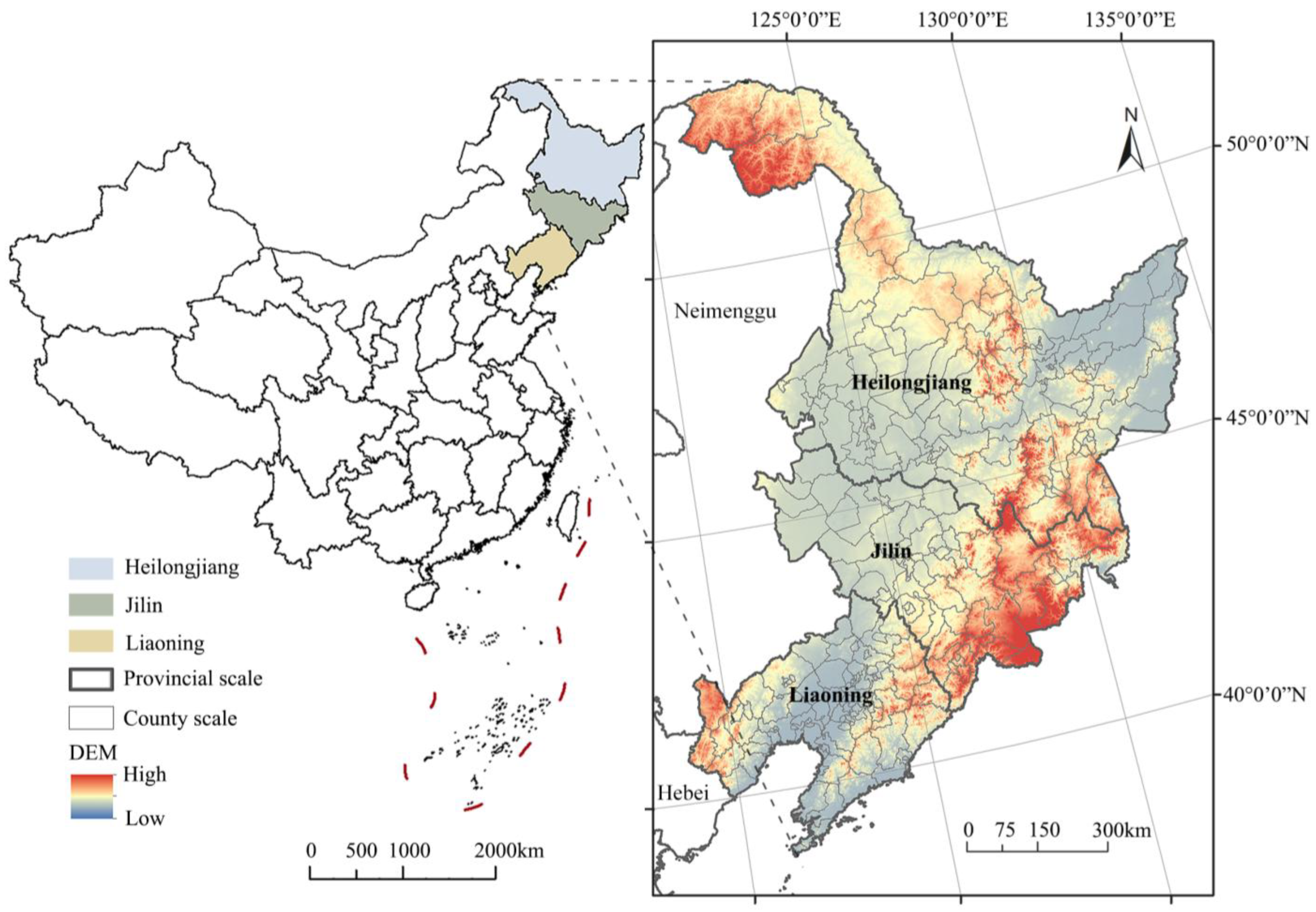
2.1. Study Area

The three northeastern provinces of China are located between 38°43′ N–53°30′ N and 115°30′ E–135°20′ E (Figure 1). As one of the country’s major grain-producing regions, the area covers approximately 787,000 km² and features a temperate monsoon climate: hot and rainy summers, and cold, dry winters. The terrain is dominated by plains and mountains, with the Changbai Mountains and the Greater and Lesser Khingan Mountains serving as natural ecological barriers. The Songnen Plain, Sanjiang Plain, and Liaohe Plain are key agricultural zones, and the region possesses the country’s most extensive black soil resources. In 2024, the total grain output of the region reached 147.68 million tons, accounting for 25% of China’s overall grain production. Meanwhile, as a traditional industrial base with a relatively high urbanization level, the region has in recent years experienced serious rural population loss and sluggish economic development. By 2024, the total GDP of the three northeastern provinces was approximately 6.345 trillion yuan, representing 4.71% of the national GDP, while the total population stood at 97.21 million—about 6.9% of the national total—marking a decrease of 12.31 million compared to 2010.

2.2. Data

The data used in this study mainly include land use datasets, provincial and county–level administrative boundary data, road and water system data, digital elevation model (DEM) data, and socio-economic data. The land use dataset was obtained from the Resource and Environment Science and Data Center of the Chinese Academy of Sciences (http://www.resdc.cn/, accessed on 11 November 2024), with a spatial resolution of 30 m. The study covers the period from 1980 to 2020, with data available at 10-year intervals (excluding 1985), resulting in four study periods. The dataset is classified into six major categories and 25 subcategories. Among them, rural settlements are a subcategory under urban, rural, industrial, and residential land, and are distinguished from urban construction land. Rural settlement patches were extracted using the ArcGIS 10.8 platform. The provincial and county administrative boundary data, as well as the transportation and river data, were obtained from the Resource and Environment Science and Data Center. The digital elevation model (DEM) data was sourced from the Geospatial Data Cloud Platform (http://www.gscloud.cn, accessed on 11 November 2024), with a spatial resolution of 30 m. Relevant socio-economic data were derived from the statistical yearbooks of the three northeastern provinces and the “China County Statistical Yearbook”. Due to data availability constraints, the socio-economic data cover the period from 2000 to 2020 and were collected at five-year intervals, including five time points: 2000, 2005, 2010, 2015, and 2020.

2.3. Methods

2.3.1. Changes in Rural Settlements

This study uses Rural Settlement Dynamics based on map overlay analysis and land use transition matrices to analyze the scale and rate of change of rural land use in the study area. The Rural Settlement Dynamics method provides the rate of change of rural settlement land use for each time period. The land use transition matrix is used to calculate the area of mutual conversion between rural settlement land and other land use types. The formulas are as follows:

$$R={\displaystyle \frac{S_{t+1}-S_t}{S_t}}\times {\displaystyle \frac{1}{T}}\times 100\%$$

(1)

In the above formula, $R$ represents the rate of change in rural settlements within the study area, $S$ denotes the area of rural settlements, $S_{t+1}$ represents the area of rural settlements at time $t+1$, $S_t$ represents the area of rural settlements at time $t$, and $T$ indicates the time interval from time $t$ to time $t+1$.

$$S_{ij}=\left[\begin{array}{ccc}a11& \dots & a1n\\ ⋮& \ddots & ⋮\\ an1& \dots & ann\end{array}\right]$$

(2)

In the above formula, $i$, $j$ ($i$, $j$ = 1, 2, …, n) represent the six major land use categories in the land use dataset, such as cultivated land, forest land, grassland, etc. $S_{ij}$ denotes the area of land converted from category $i$ to category $j$.

2.3.2. Average Nearest Neighbor Analysis and Kernel Density Analysis

(1)

Average nearest neighbor index

The Average Nearest Neighbor Index is a statistical measure used to assess the degree of spatial clustering in point data. It evaluates the distribution pattern of points by calculating the distance from each point to its nearest neighbor and then averaging these distances. This method can be implemented using the spatial analysis tools in ArcGIS. The corresponding formula is as follows:

$$ANN={\displaystyle \frac{\overline{D_0}}{\overline{D_e}}}={\displaystyle \frac{{\sum }_{i=1}^n{d}_i/n}{\sqrt{A/n}/2}}$$

(3)

In the formula above, $\overline{D_0}$ represents the observed mean distance between the centroids of each rural settlement patch and its nearest neighbor, $\overline{D_e}$ denotes the expected mean distance under a random distribution pattern, $n$ is the total number of rural settlement patches, $d_i$ is the distance from point $i$ to its nearest neighbor, $A$ is the area of the minimum bounding rectangle encompassing all settlement patches. When the ANN value is less than 1, the distribution pattern is considered clustered; when the ANN value is greater than 1, the pattern tends toward dispersion.

(2)

Kernel density analysis

Kernel density analysis is a commonly used non-parametric method for estimating the probability density function of a random variable. In spatial analysis, it is primarily used to calculate the density of target features (such as point or line features) within their surrounding neighborhood, thereby reflecting the spatial distribution characteristics of the data. The formula is as follows:

$$f(x)={\displaystyle \frac{1}{nh}}{\displaystyle \sum }_{i=1}^{n}k\left({\displaystyle \frac{x-x_i}{h}}\right)$$

(4)

In the formula above, $f\left(x\right)$ is the kernel function, which estimates the density at location $x$. $n$ is the total number of sample points; $x_i$ indicates the coordinate of the i-th observation; $h$ is the smoothing parameter that reflects the distance between individual elements, and ($x-x_i$) represents the distance between the estimation point $x$ and the observation point $x_i$.

2.3.3. Spatial Correlation Index

(1)

Spatial Autocorrelation Tool (Global Moran’s I)

Spatial autocorrelation analysis is a statistical method used to assess whether the spatial distribution pattern of a given variable is clustered, dispersed, or random. The formula is as follows:

$$I={\displaystyle \frac{n}{S_0}}{\displaystyle \frac{{\sum }_{i=1}^n{\sum }_{j=1}^n{w}_{i,j}{z}_i{z}_j}{{\sum }_{i=1}^n{z}_i^2}}$$

(5)

In the above formula, $n$ represents the total number of features, $S_0$ denotes the sum of all spatial weights, $z_i$ is the deviation of the attribute value of feature $i$ from the mean, and $w_{i,j}$ represents the spatial weight between features $i$ and $j$.

(2)

Hotspot/Coldspot Analysis (Getis–Ord General G)

The Getis–Ord General G statistic is used to measure the clustering of high or low values within the study area, helping to analyze the global spatial distribution patterns of rural settlements. The formula is as follows:

$$G(d)={\displaystyle \frac{{\sum }_{i=1}^n{\sum }_{j=1}^n{w}_{ij}(d)x_i{x}_j}{{\sum }_{i=1}^n }}$$

(6)

In the formula, $w_{ij}$ represents the spatial weight between features $i$ and $j$ based on a distance-based rule, $x_i$ and $x_j$ are the observed values of features $i$ and $j$, and $n$ denotes the number of features in the dataset.

(3)

Hot Spot Analysis

Hot spot analysis visualizes the spatial locations of high–or low–value features within the study area, allowing for the significant identification of the scale differentiation characteristics of rural settlement clustering. The calculation is based on the following formula:

$$G*(d)={\displaystyle \frac{{\sum }_{j=1}^n{w}_{ij}(d)x_i{x}_j}{{\sum }_{j=1}^n{x}_j}}$$

(7)

In the above formula, the meanings of $w_{ij}$, $x_i$, $x_j$, and $n$ are consistent with those in Formula (6). By standardizing G*(d) to obtain Z(G*), a positive Z–score indicates a high–value clustering of rural settlements within the area, while a negative Z–score suggests a low-value clustering.

2.3.4. Morphology Characteristics Based on Landscape Pattern Index

Landscape pattern indices are a set of quantitative metrics used to analyze the spatial structural characteristics of landscapes. They reflect the morphology, scale, and spatial distribution of land cover types within a given area. Based on existing literature [15,26], this study explores the scale and morphological evolution of rural settlements in the three northeastern provinces of China from 1980 to 2020 using eight selected indices from two dimensions: scale and shape. These indices include class area (CA), number of patches (NP), patch density (PD), mean patch size (MPS), largest patch index (LPI), area-weighted mean shape index (AWMSI), area-weighted mean patch fractal dimension (AWMPFD), and aggregation index (AI). The definitions and explanations of these indices are shown in

Table 1. Landscape indices and ecological significance.

Dimension	Index Names	Abbreviations	Significance
Scale characteristics	Class area	CA	Overall area of a particular patch type.
	Number of patches	NP	The total number of patches (NP) for a specific patch type within the landscape
	Patch density	PD	The density of specific patch types provides insights into landscape heterogeneity and fragmentation, serving as a key indicator of heterogeneity per unit area.
	Largest patch index	LPI	The Largest Patch Index quantifies the percentage of total landscape area occupied by the largest patch of a specific patch type, serving as a crucial indicator of landscape dominance and fragmentation patterns.
	Mean patch size	MPS	The Mean Patch Size, calculated as the total area of a specific patch type divided by its number of patches, serves as a fundamental metric for quantifying landscape fragmentation and habitat connectivity
Morphological characteristics	Area–weighted mean shape index	AWMSI	The Area-Weighted Mean Shape Index quantifies the complexity of patch shapes by considering both the geometric form and relative area contribution of individual patches, providing a comprehensive assessment of landscape configuration
	Area–weighted mean patch fractal dimension	AWMPFD	The Area-Weighted Mean Patch Fractal Dimension quantifies the geometric complexity of landscape patterns by incorporating both the shape irregularity and area contribution of individual patches, providing a robust measure of spatial heterogeneity across multiple scales
	Aggregation index	AI	The Aggregation Index examines the connectivity between patches of each landscape type. The smaller the value, the more discrete the landscape

.

2.3.5. Indicator Selection for Driving Factors Research

Based on previous studies [22,38,58], and considering the regional context of the three northeastern provinces as a major grain-producing area dominated by agricultural rural settlements [20], this study selects 12 influencing factors from two dimensions—natural factors and socio-economic factors—to explore the driving mechanisms behind rural settlement evolution. Descriptions of the selected factors are provided in

Table 2. Description of selected factors.

Dimension		Factors	Factor Descriptions
Natural factors		Elevation	The altitude at which the rural settlement is located
		Distance from water system	The Euclidean distance of rural settlements from the nearest water system (e.g., rivers, lakes, or reservoirs)
		Distance from road networks	The Euclidean distance of rural settlements from the nearest main roads or transportation networks
Socioeconomic factors	Demographic factors	Rural population (RP)	The total number of residents living in rural areas within the region
		Urbanization rate (UR)	The ratio of the urban population to the total population of the region, indicating the level of urbanization
	Agricultural productivity factors	Total power of agricultural machinery (TPAM)	The combined power capacity of all agricultural machinery used in the region for farming and related activities
		Total grain output (TGO)	The total yield of grains produced by agricultural producers and operators within the region
	Economic factors	Regional gross domestic product (GDP)	The total monetary value of all goods and services produced within the region in a specific time period
		Value added of primary industry (VAPI)	The value added of the primary industry refers to the newly created value during the production process of agriculture, forestry, animal husbandry, and fishery
		GDP per capita (GDP-PC)	The regional GDP divided by the permanent resident population, representing the average economic output per person.
		Total industrial output value of enterprises above designated size (TIOV-EDS)	The total production value of industrial enterprises that meet or exceed a specific size threshold
	Social factors	Administrative area (AA)	The total land area under the jurisdiction of the administrative region.

.

2.3.6. XGBoost Model and SHAP

(1)

Extreme Gradient Boosting Model (XGBoost)

XGBoost is an optimized gradient boosting decision tree algorithm that combines multiple weak learners to form a powerful ensemble model. It offers significant advantages in handling non-linear relationships, modeling interaction effects among variables, evaluating feature importance, resisting overfitting, automatically managing missing values, and allowing flexible parameter tuning. These capabilities enable XGBoost to produce accurate, efficient, and reliable analytical results while effectively capturing the complex relationships between feature variables and the target variable [49]. The objective function consists of a training loss function and a regularization term, and is defined as follows:

$$Obj={\displaystyle {\displaystyle \sum }_{i=1}^n}l(\stackrel{\wedge }{y_i},y_i)+{\displaystyle {\displaystyle \sum }_{k=1}^K}\Omega (f_k)$$

(8)

In the above formula, $l(\stackrel{\wedge }{y_i},y_i)$ represents the loss function, $\stackrel{\wedge }{y_i}$ denotes the predicted value for the sample $x_i$, and $y_i$ is the true value. The term $\Omega \left(f_k\right)$ is the regularization term, which quantifies the complexity of the weak learners. $n$ is the total number of samples, and $K$ represents the total number of trees in the model.

(2)

Shapley Additive Explanations (SHAP)

SHAP is a widely used post-hoc model-agnostic interpretability method for machine learning algorithms. Its core idea is to compute the marginal contribution of each feature to the model’s output, which is equivalent to the influence of that feature on a given sample. Based on Shapley values from cooperative game theory, SHAP decomposes the model’s prediction into the sum of the marginal contributions of each input feature. The formula is as follows:

$$\stackrel{\wedge }{y_i}=f_0+{\displaystyle \sum }_{i=1}^M{f}_i$$

(9)

In the formula, $f_0$ represents the average prediction of all samples in the training dataset, $f_i$ denotes the marginal contribution of each feature, and $M$ is the total number of features.

3. Results

3.1. Characteristics of Land Use Changes in Rural Settlements

From 1980 to 2020, the total area converted from other land use types to rural settlements reached 132,379.62 km². Among these, arable land and forests were the two major sources of conversion to rural settlements (

Table 3. Area of change between rural settlements and other land use types from 1980 to 2020.

Area of Other Land Use Types Converted to Rural Settlements			Area of Rural Settlements Converted to Other Land Use Types
Land Use Types	Area (km2)	Percentage (%)	Land Use Types	Area (km2)	Percentage (%)
Arable land	66,619.95	50.32	Arable land	28,880.08	21.21
Forests	24,157.23	18.24	Forests	41,337.38	30.36
Grassland	12,916.32	9.75	Grassland	35,277.89	25.91
Water bodies	5758.94	4.35	Water bodies	10,300.23	7.56
Urban built–ups	3725.71	2.81	Urban built-ups	311.48	0.23
Other construction land	2165.88	1.63	Other construction land	782.52	0.57
Unused land	17,035.57	12.87	Unused land	19,272.06	14.15
Total	132,379.63	100	Total	136,161.64	100

). Arable land contributed the most, with an area of 66,619.95 km², accounting for 50.32% of the total converted area, followed by forest land with an area of 24,157.23 km², accounting for 18.24%. Meanwhile, the total area of rural settlements converted to other land use types during the same period was 136,161.63 km². Forests, grassland, and arable land were the top three destinations of this outflow, accounting for 30.35%, 25.90%, and 21.21% of the total outflow, respectively. The overall mutual conversions among the eight land use types are illustrated in Figure 2.

During the study period, the scale of rural settlements in the three northeastern provinces of China exhibited significant dynamic evolution. The total settlement area increased from 17,051.37 km² to 20,837.04 km², with a net growth of 3785.66 km², demonstrating an overall stepped expansion trend. The spatial evolution of rural settlements followed a four-stage trend of “expansion–stabilization–re–expansion–restabilization”. Among them, the period from 1980 to 1990 was one of rapid expansion, with an increase of 1595.28 km² and a change rate of 0.94%, the highest among all intervals. The second most significant growth occurred between 2000 and 2010, with an expansion of 1550.36 km² and a change rate of 0.82%. In contrast, the periods of 1990–2000 and 2010–2020 saw relatively slower expansion, with area increases of 310.74 km² and 329.29 km², and corresponding change rates declining to 0.17% and 0.16%, respectively. Notably, 2010–2020 marked the lowest growth rate during the study period. Detailed statistics on rural settlement area and change rates for each time period are presented in

Table 4. Area and dynamics of rural settlements from 1980 to 2020.

Research Year	Area of Rural Settlements (km2)	Changes in Area (km2)	Rural Settlement Dynamics (%)
1980	17,051.37	-	-
1990	18,646.65	1595.28	0.94
2000	18,957.39	310.74	0.17
2010	20,507.75	1550.36	0.82
2020	20,837.04	329.29	0.16

.

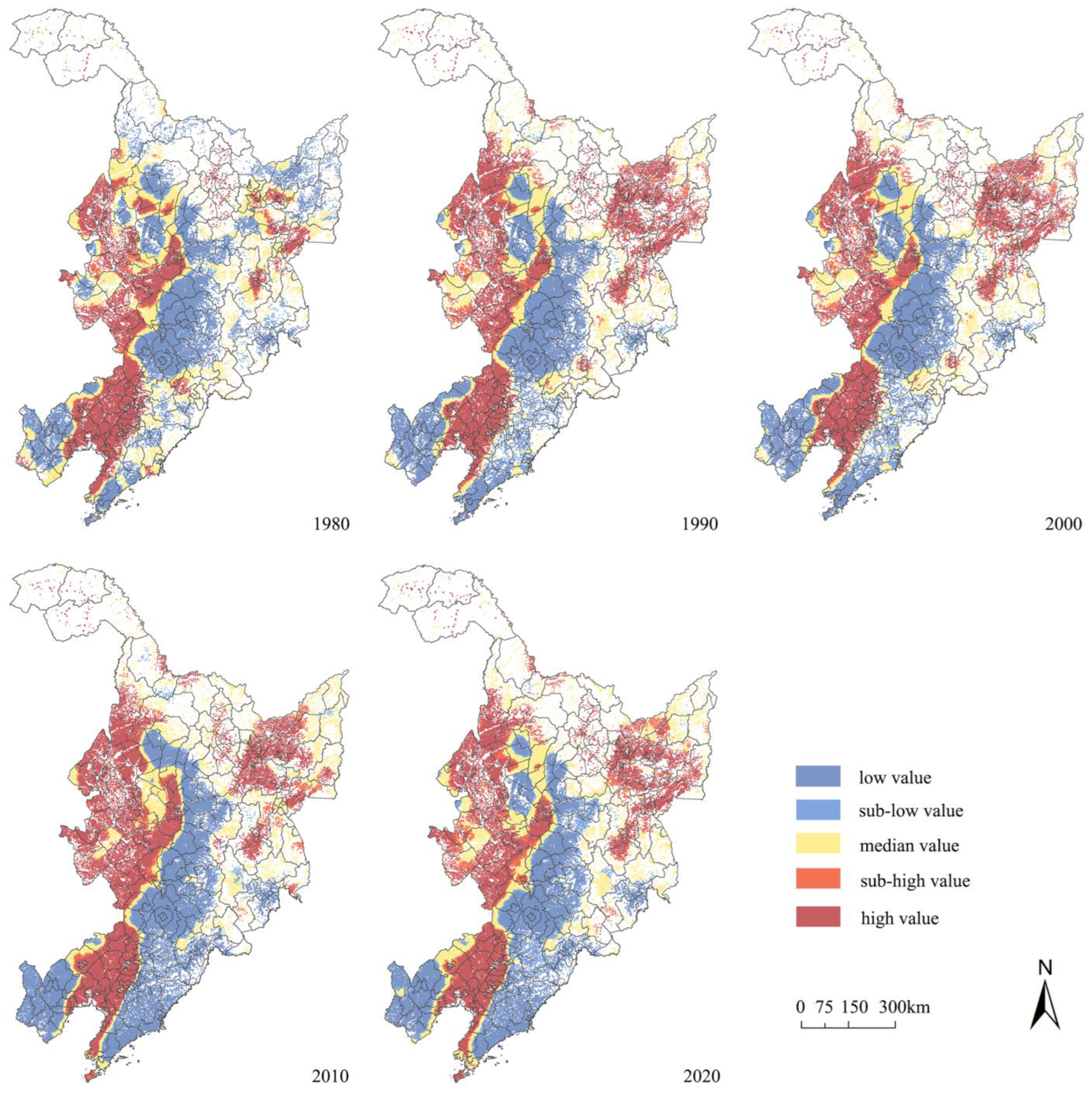
3.2. Analysis of Rural Spatial Evolution Characteristics

This study analyzes the average nearest neighbor (ANN) index of rural settlements in the three northeastern provinces from 1980 to 2020, as shown in

Table 5. ANN index of villages and towns in TNPs from 1980 to 2020.

Research Year	ANN Index	Z-Score	p
1980	0.528	−304.522	0.000
1990	0.590	−251.042	0.000
2000	0.590	−250.986	0.000
2010	0.613	−260.713	0.000
2020	0.602	−264.668	0.000

. Throughout the period, all ANN indices stayed below 1, showing that rural settlements followed a clustered spatial pattern. From 1980 to 2020, the ANN index rose from 0.528 to 0.602, which means the clustering became slightly weaker over time, but rural settlements still maintained a clear agglomeration trend.

The kernel density distribution of rural settlements in Northeast China from 1980 to 2020 is shown in Figure 3. Overall, the spatial distribution of rural settlements gradually evolved from “single–center clustering” to “multiregional contiguous clustering”. From 1980 to 2000, high-density areas of rural settlements were concentrated in the Songnen Plain, covering southern Heilongjiang and central Jilin and including Gongzhuling City, Changyi District, Chuanying District, Shuangyang District, Jiutai District, Yongji County, and Lishu County. These high-density clusters remained relatively stable in spatial location, although their kernel density values tended to decrease. From 2000 to 2020, high-density zones expanded in western and southern Liaoning, forming two new medium-to-high-density core areas involving Zhuanghe City, Pulandian District, Jianchang County, and Chaoyang County. Meanwhile, the high-density zones in the Songnen Plain experienced a continuous decline. These three high-density areas exhibited a contiguous spatial distribution. Compared with 1980, in 2020, rural settlements in the southern part of the study area presented increased clustering and continuity, whereas the clustering levels in the central and eastern regions declined. The spatial pattern of rural settlements shifted from a highly concentrated, single-center to a multicenter, regionally coordinated structure.

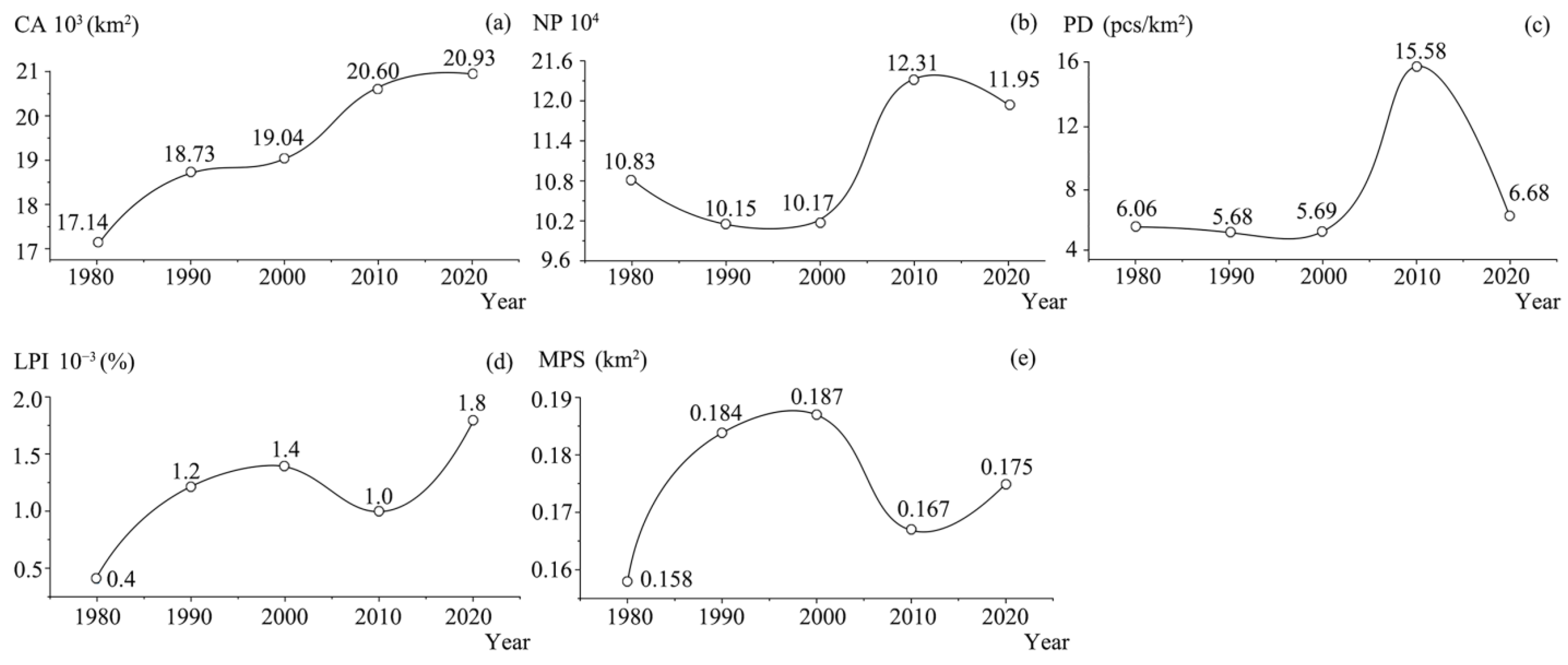
3.3. Scale Evolution Characteristics of Rural Settlements

3.3.1. Characteristics of Scale Increase and Decrease

The calculation results of the scale increase and decrease of rural settlements are shown in

Table 6. Characteristics of scale increase and decrease in TNPs from 1980 to 2020.

Research Year	CA (km2)	NP	PD (pcs/km2)	LPI	MPS (km2)
1980	17,148.36	108,390	6.06	0.0004	0.158
1990	18,738.60	101,520	5.68	0.0012	0.184
2000	19,049.71	101,784	5.69	0.0014	0.187
2010	20,602.41	123,104	15.58	0.001	0.167
2020	20,932.86	119,526	6.68	0.0018	0.175

. Combined with the Scale Change Index Map (Figure 4), it can be observed that from 1980 to 2020, CA exhibited a steady annual increase, while MPS showed a fluctuating upward trend. Overall, CA increased by 22%, and MPS increased by 13%, indicating a continuous expansion in the land area occupied by rural settlements. In addition, the LPI also displayed a general upward trend, suggesting that rural settlements tended to develop in a more clustered manner spatially. NP increased in a fluctuating pattern, peaking in 2010, with a total increase of 10.2%. The trend of PD was consistent with that of NP, ranging between 5.6 and 15.6. These two indicators collectively reflect a growing degree of fragmentation in rural settlement patterns.

3.3.2. Characteristics of Scale Differentiation

Table 7. Spatial autocorrelation analysis.

Research Year	Moran’s I	Z-Score	p
1980	0.098	243.599	0.000
1990	0.088	357.061	0.000
2000	0.084	342.691	0.000
2010	0.090	435.936	0.000
2020	0.054	230.523	0.000

presents the Moran’s I values for the standard deviation of rural settlement patch areas in the three northeastern provinces. Throughout the study period, the indices remained significantly positive, indicating a clear spatial clustering in the size distribution of rural settlements. However, since Moran’s I does not distinguish between clusters of high and low values, we further employed the Getis-Ord General G statistic to analyze the spatial patterns (

Table 8. Global spatial clustering test.

Research Year	Z-Score	p
1980	−6.213	0.000
1990	−19.909	0.000
2000	−18.491	0.000
2010	−14.651	0.000
2020	−13.117	0.000

). The results show that all Z-scores were negative during the study period, suggesting a more prominent clustering of low values. This indicates the widespread presence of low-value clusters dominated by small-scale settlement patches across the study area.

We used the “hot spot analysis” tool in ArcGIS 10.8 to visualize the spatial differentiation of rural settlement scales across the study area, which led to the generation of five-period hotspot distribution maps from 1980 to 2020 (Figure 5). The results reveal significant spatial changes in the Sanjiang Plain, northern Songnen Plain, and lower Liaohe River Basin. In 1980, rural settlements were mainly scattered as isolated points or small patches across most areas, with relatively loose spatial patterns and no large-scale clustering, except for parts of the Songnen and Liaohe Plains. Between 1980 and 1990, high-value clusters of rural settlements gradually expanded, particularly in the central Sanjiang Plain and northern Songnen Plain, forming distinct hotspots including Fujin City, Nehe City, Nenjiang City, Suibin County, Luobei County, Baoqing County, Boli County, Huachuan County, and Jixian County. After 1990, the spatial distribution of hot and cold spots remained relatively stable. From 2000 to 2010, the high-value agglomeration area further expanded to include Wangkui County, Lanxi County, Da’an City, and Taonan City. Meanwhile, low-value clusters in the lower Liaohe Plain significantly intensified in both scale and aggregation; these included Huairen County, Xinbin County, Kuandian County, Fengcheng City, Xiuyan County, Donggang City, and Zhuanghe City. From 2010 to 2020, some of the high-value agglomerations in the Songnen Plain, including Baiquan County and Hailun City, exhibited a shrinking trend. However, the overall pattern of rural settlement hot and cold spots across the study area continued to present large-scale clustering. Overall, from 1980 to 2020, rural settlements in the Sanjiang Plain and northern Songnen Plain evolved into large-scale clusters dominated by large patches, whereas those in the lower Liaohe River Basin developed into large-scale clusters composed primarily of small patches.

3.4. Analysis of the Morphological Characteristics of Rural Settlements

This study analyzes the morphological characteristics of rural settlements from two perspectives: the overall patch characteristics and the individual shape features of the settlements. AWMSI and AWMPFD represent the intrinsic morphological features of settlement patches, while AI reflects the overall spatial pattern of the settlements. The relevant calculation results are presented in

Table 9. Landscape index table of morphological characteristics in TNPs from 1980 to 2020.

Research Year	AWMSI	AWMPFD	AI (%)
1980	1.558	1.069	89.958
1990	1.526	1.065	90.747
2000	1.530	1.065	90.823
2010	1.569	1.070	90.033
2020	1.610	1.072	90.317

. Combined with the index variation shown in Figure 6, AWMSI decreased initially and then increased from 1980 to 2020. It reached its lowest value of 1.52 in 1990 and showed a continuous upward trend thereafter, reaching 1.61 in 2020. This indicates that the shapes of rural settlement patches have become increasingly irregular. AWMPFD remained close to 1 throughout the study period, with minimal fluctuations, suggesting weak fractal characteristics and a high degree of influence from anthropogenic factors. AI, which measures the degree of spatial aggregation of rural settlements, increased from 1980 to 2000, declined between 2000 and 2010, and then rose again from 2010 to 2020, peaking at 90.82 in 2000. Overall, AI exhibited a fluctuating trend, ranging from 89.9 to 90.3, indicating a slight increase in aggregation over time. These results suggest that, driven by urbanization, rural settlements in the study area have evolved toward more irregular shapes and increasingly clustered spatial patterns.

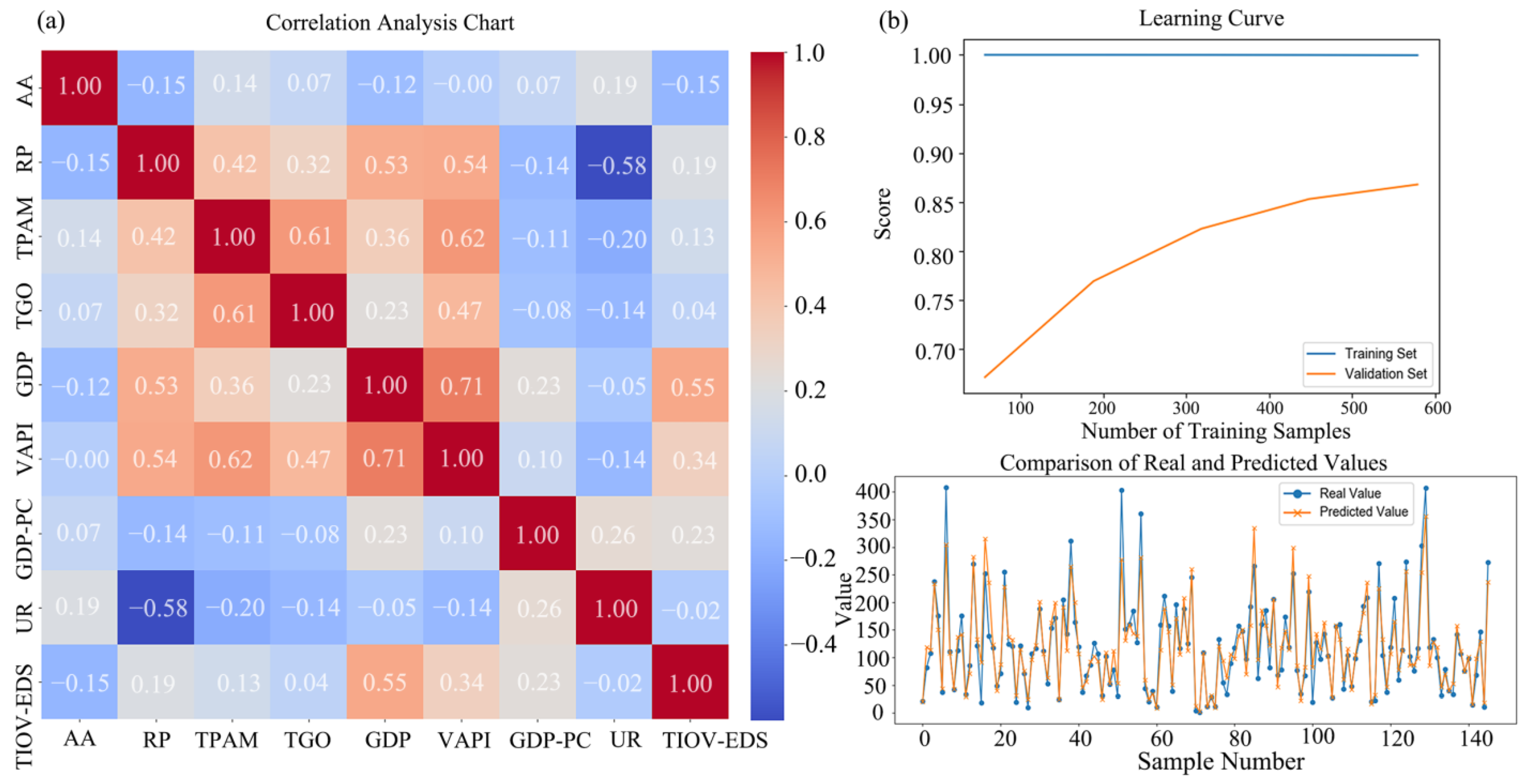
3.5. Analysis of Driving Factors of Rural Settlements

3.5.1. Natural Factors

Elevation

We categorized the region into three elevation levels, 0–500 m, 500–1000 m, and 1000–2000 m, and the results of the landscape pattern index calculations are shown in

Table 10. Settlement landscape characteristics of villages and towns at different elevations in the buffer zone of TNPs from 1980 to 2020.

Factors	0–500 m			500–1000 m			1000–2000 m
	1980	2000	2020	1980	2000	2020	1980	2000	2020
CA (km2)	16,844.99	18,703.40	20,458.01	316.47	362.85	490.36	0.81	1.15	1.92
NP	107,852	100,334	116,696	3366	3254	5084	16	11	23
PD (pcs/km2)	6.402	5.364	5.704	10.636	8.967	10.367	19.750	9.565	11.979
LPI	0.001	0.0039	0.0052	0.0001	0.0028	0.0033	0	0.002	0.0021
MPS (km2)	0.156	0.186	0.175	0.094	0.112	0.096	0.050	0.105	0.083
AWMSI	1.626	1.608	1.684	1.656	1.657	1.697	1.571	1.531	1.528
AWMPFD	1.076	1.073	1.079	1.081	1.079	1.084	1.082	1.073	1.075
AI (%)	86.287	87.400	86.827	83.400	84.871	83.196	80.611	86.569	84.448

. Among the three elevation zones, the average values of CA, NP, LPI, and MPS are highest within the 0–500 m range and show an increasing trend. In contrast, these indices decline sharply at elevations of 500–1000 m and 1000–2000 m. These findings indicate that rural settlements are more numerous and larger in scale in lower-elevation areas. PD exhibits the lowest average value in the 0–500 m elevation range, but its values significantly increase in the two higher elevation ranges. AI displays high values at 0–500 m and low values at 500–1000 m, but its values rebound to elevated levels at 1000–2000 m. These findings indicate that rural settlements in high-elevation areas adopt a small-scale, high-agglomeration pattern. AWMSI and AWMPFD present lower average values in high-elevation areas than in low-elevation zones, and AWMSI shows an expanding trend in low-elevation regions. This finding indicates that rural settlements in low-elevation areas tend to have irregular morphologies, whereas those in high-elevation areas display relatively regular shapes.

Distance from the Water System

We established multiple buffer zones at distances of 0–2 km, 2–4 km, and 4–6 km to analyze the spatial differentiation characteristics of rural settlements using landscape pattern indices (

Table 11. Settlement landscape characteristics of villages and towns with different distances from the river system buffer zones in TNPs from 1980 to 2020.

Factors	0–2 km			2–4 km			4–6 km
	1980	2000	2020	1980	2000	2020	1980	2000	2020
CA (km2)	5382.04	5875.46	6586.21	4140.02	4535.31	4963.89	2845.91	3120.24	3406.84
NP	38,659	36,964	43,841	33,661	32,308	37,830	22,397	21,483	25,021
PD (pcs/km2)	7.182	6.291	6.656	8.130	7.123	7.621	7.869	6.885	7.346
LPI	0.0031	0.0079	0.0074	0.0029	0.004	0.004	0.004	0.0048	0.0089
MPS (km2)	13.922	15.895	15.023	12.299	14.038	13.122	12.707	14.524	13.616
AWMSI	1.533	1.515	1.585	1.520	1.499	1.560	1.523	1.496	1.547
AWMPFD	1.067	1.065	1.071	1.067	1.064	1.070	1.067	1.064	1.069
AI (%)	89.578	90.303	89.787	89.044	89.803	89.206	89.198	89.979	89.444

). Across the three buffers, the average values of CA, NP, LPI, and MPS were highest within the 0–2 km buffer from the water system and tended to increase. In contrast, PD presented the lowest average value in the 0–2 km range, whereas AI presented consistently high values with minimal variation across all buffers. These results indicate that rural settlements located farther from water bodies tend to exhibit a small-scale, high-agglomeration pattern. In terms of morphological indices, AWMSI and AWMPFD showed little variation, which suggests that water systems have a limited influence on settlement shape.

Distance from Road Networks

Roads serve as crucial connectors between rural settlements. To investigate how the distance between rural settlements and roads influences the settlement spatial distribution, we established buffer zones at 0–2 km and 2–4 km and conducted an analysis using landscape pattern indices. As shown in the analysis results in

Table 12. Landscape characteristics of villages and towns with different distances from road buffer zones in TNPs from 1980 to 2020.

Factors	0–2 km			2–4 km
	1980	2000	2020	1980	2000	2020
CA (km2)	8704.31	9710.21	10,485.80	3485.36	3792.16	4141.78
NP	54,997	51,268	57,144	29,891	28,882	33,430
PD (pcs/km2)	6.318	5.279	5.449	8.577	7.616	8.072
LPI	0.0026	0.003	0.0077	0.002	0.0022	0.0054
MPS (km2)	0.158	0.189	0.183	0.116	0.131	0.123
AWMSI	1.579	1.552	1.642	1.488	1.464	1.519
AWMPFD	1.07	1.066	1.073	1.065	1.062	1.067
AI (%)	90.164	91.071	90.761	88.735	89.424	88.887

, the values of CA, NP, LPI, MPS, and AI are high within the 0–2 km buffer zone and show an increasing trend, which indicates that rural settlements located closer to roads tend to be large in scale and fairly concentrated. In contrast, the value of PD is greater in the 2–4 km buffer zone, while the decrease in AI is relatively limited; this suggests that settlements farther from roads exhibit a small-scale, high-agglomeration pattern. With respect to shape characteristics, AWMSI and AWMPFD also exhibit high values and an increasing trend within the 0–2 km buffer, which indicates that settlements close to roads tend to have irregular shapes, whereas those farther away appear more regular in form.

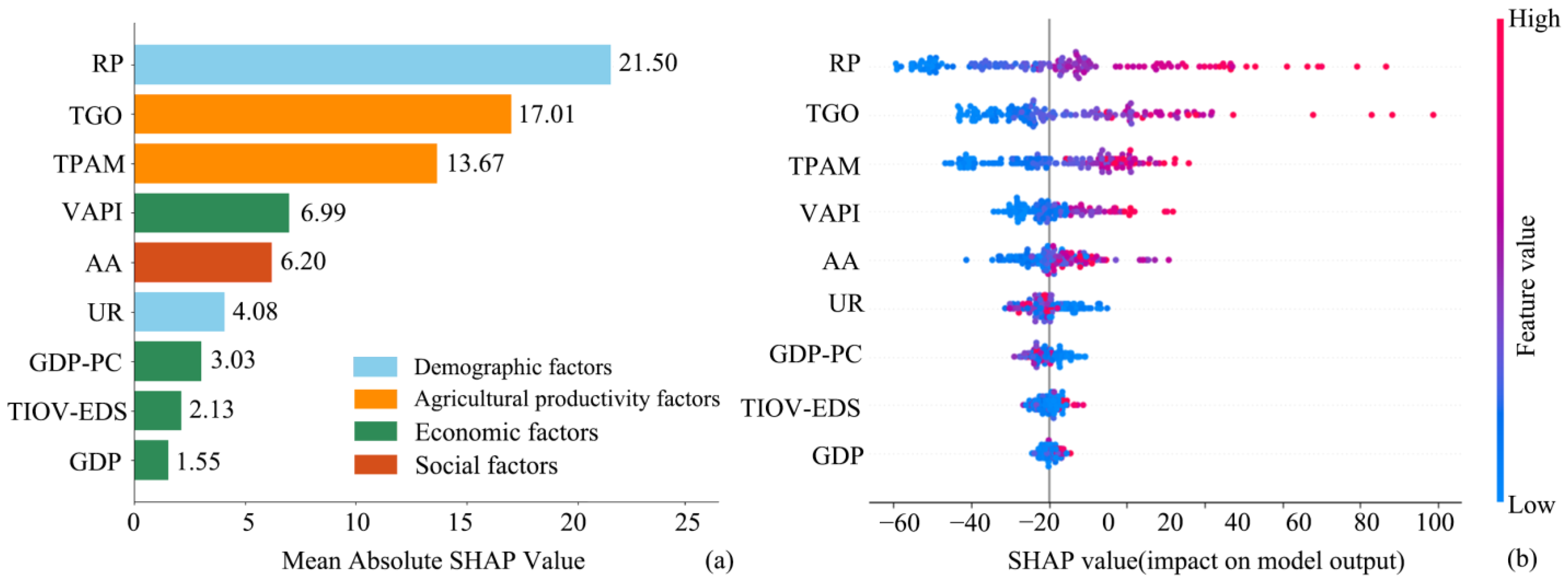
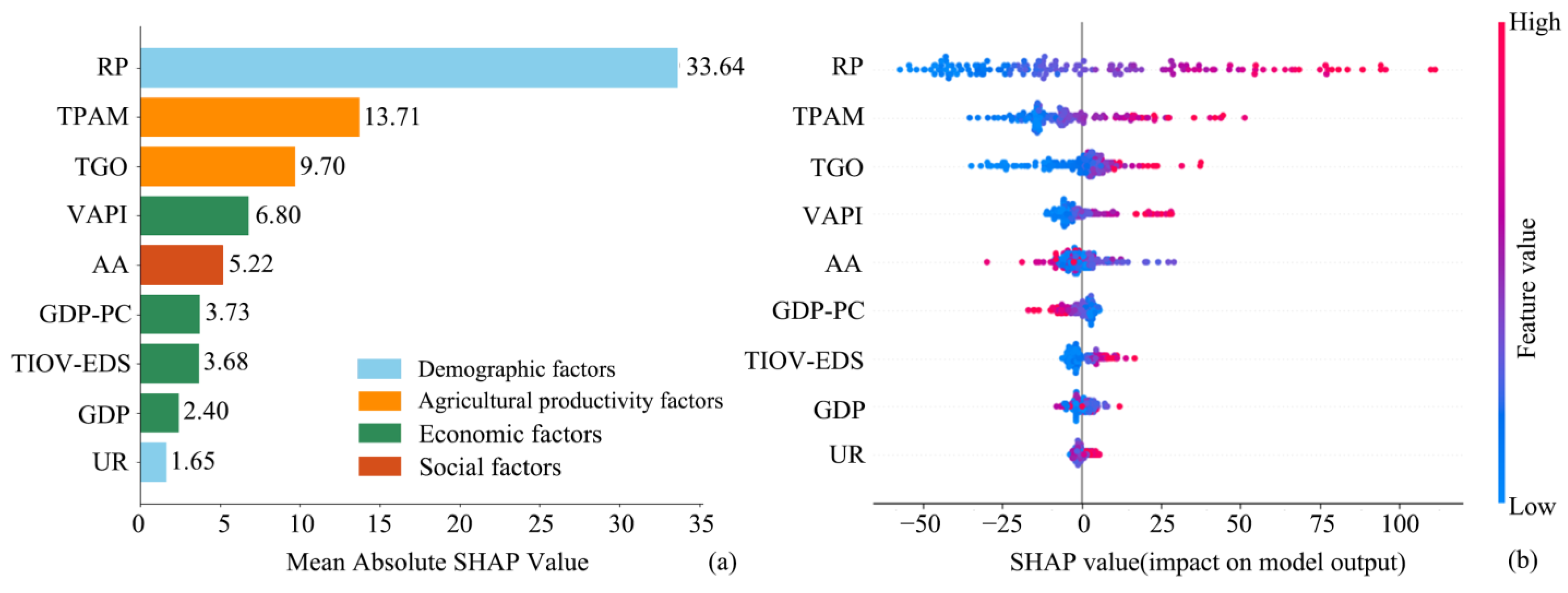
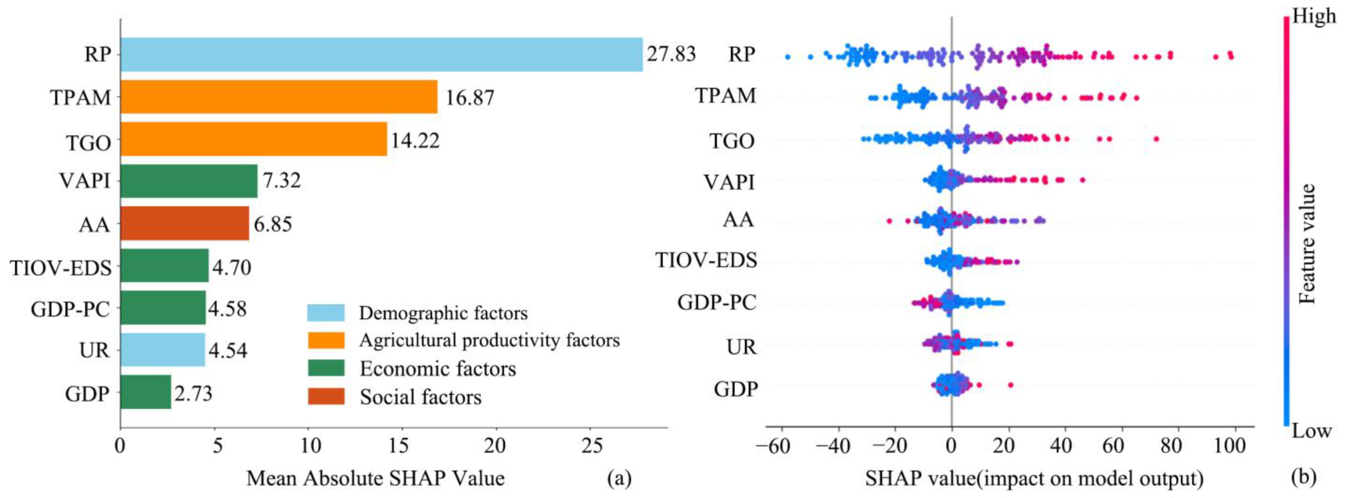
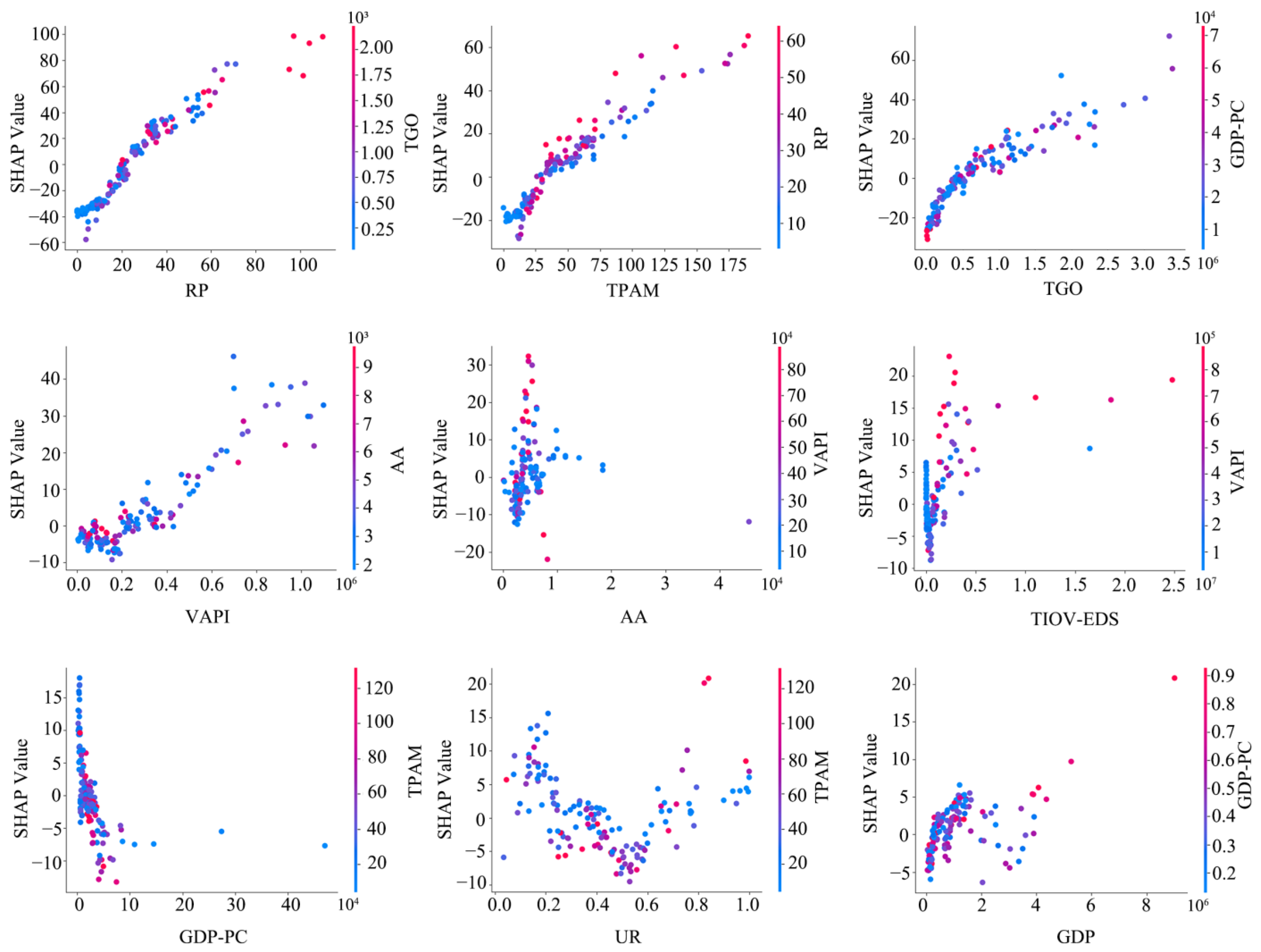
3.5.2. Socioeconomic Factors

To reveal the impact of socioeconomic factors on the spatial evolution of rural settlements in the study area as a whole and across different periods, nine socioeconomic variables were selected with consideration of the data availability and representativeness of the indicators. These variables include the administrative area (AA), the rural population (RP), the total power of agricultural machinery (TPAM), the total grain output (TGO), the regional gross domestic product (GDP), the value added of the primary industry (VAPI), GDP per capita (GDP-PC), the urbanization rate (UR), and the total industrial output value of enterprises above designated size (TIOV-EDS). After addressing missing data through linear interpolation or exclusion, we included a total of 146 county-level units in the model.

In this study, we employed the XGBoost model and divided the research period into two intervals: 2000–2010 and 2010–2020. Prior to model construction, we conducted a correlation analysis on all independent variables. The results are shown in Figure 7a, which reveals no significant collinearity issues among the variables. The prediction model was developed using the 2000–2015 dataset as the training set, which included four time points: 2000, 2005, 2010, and 2015. The 2020 dataset was used as the test set. The ratio of the training set to the test set was 4:1. Figure 7b presents the model’s training progress. To ensure robustness, three-fold cross-validation was applied. The optimal hyperparameters obtained through grid search were: colsample_bytree = 1.0, learning rate = 0.01, max depth = 7, n_estimators = 500, and subsample = 0.8.

Table 13. Performance comparison of different machine learning models.

Model	R2	RMSE (km2)	MAE (km2)
Extreme Gradient Boosting (XGBoost)	0.88	33.09	25.26
Random Forest (RF)	0.82	36.14	25.64
Support Vector Machine (SVM)	0.75	42.20	30.80

compares the performance of XGBoost with Random Forest (RF) and Support Vector Machine (SVM). Among the three models, XGBoost achieved the best performance across all evaluation metrics. It yielded the highest R² value (0.88), indicating a stronger ability to explain the variance in rural construction land area. Additionally, its RMSE (33.09 km²) and MAE (25.26 km²) were the lowest, suggesting more accurate and stable predictions. These results demonstrate that XGBoost is a more suitable model for analyzing the complex, nonlinear relationships among the driving factors of rural spatial evolution.

We conducted SHAP global and local importance analyses on all feature variables. Figure 8a, Figure 9a, and Figure 10a illustrate the global SHAP feature importance, which is calculated across all samples and ranked by the mean absolute SHAP value of each variable in descending order. Panel (b) in each figure presents the SHAP summary plot, in which the SHAP values of each feature for individual samples are visualized, indicating both the magnitude and direction of feature influence. In these plots, the x-axis represents the SHAP value, while the y-axis lists the feature variables. Each dot in the plot represents the SHAP value of a single sample, and its color indicates the original feature value—purple for high values and blue for low values. When high feature values are distributed on the positive side of the x-axis, the corresponding variable exerts a positive effect on the target variable; conversely, when they appear on the negative side, the effect is negative. Figure 8 presents the importance analysis of socioeconomic variables in the three northeastern provinces of China during the 2000–2010 period. The results indicate that the UR and GDP-PC had a negative effect on the rural settlement scale, whereas all other variables had a positive effect. Among them, the RP had the greatest influence, with an importance value of 21.50. The TGO and TPAM ranked second and third, with importance values of 17.01 and 13.67, respectively. Among the economic variables, the VAPI ranked fourth, with an importance value of 6.99, followed by the AA at 6.20, which also exerted a positive influence. The UR ranked sixth and had a notable negative effect, which may be attributed to the decrease in the rural population driven by urbanization. In addition, the remaining economic variables—GDP-PC, the TIOV-EDS, and GDP—exhibited relatively low importance, with values of 3.03, 2.13, and 1.55, respectively. Notably, GDP-PC appeared to be negatively correlated with the rural settlement scale, possibly because GDP per capita is disproportionately influenced by urban residents, whose income levels are significantly higher than those of rural residents. From 2010 to 2020, the importance of influencing factors exhibited both consistency and variation compared with the previous study period (Figure 9). The population remained the dominant influencing factor, with an importance value of the RP reaching 33.64. The importance ranking of the TPAM increased to second place, with a value of 13.71, followed by the TGO, with a value of 9.70. The rankings of the VAPI and AA remained unchanged, with importance values of 6.80 and 5.22, respectively. Notably, the AA had a certain degree of negative impact on the rural settlement scale. In addition, the UR decreased to the lowest level of importance, with a value of only 1.65. This decline may be attributed to the continued advancement of urbanization, which resulted in a relatively high level of urbanization in the region and a slowing growth rate, thus reducing the extent of urban spillover effects on rural areas. The importance values of GDP-PC, the TIOV-EDS, and GDP remained low, with GDP-PC showing a clear negative effect. This finding indicates that during the study period, the development of the secondary and tertiary sectors had a limited influence on changes in the rural settlement scale in the three northeastern provinces of China. Figure 10 presents the calculated importance of various factors influencing rural settlement scale changes from 2000 to 2020. Demographic factors and agricultural productivity factors emerged as the top two contributors, with both exerting positive effects on the rural settlement scale. Among economic factors, the VAPI stood out as the most influential. In contrast, the TIOV-EDS, GDP-PC, the UR, and GDP had relatively limited effects on rural settlement changes, with GDP-PC and the UR showing a certain degree of negative impact.

On the basis of the global and local SHAP importance analysis of the factors influencing rural settlement spatial evolution, we further employed SHAP dependence plots to investigate the marginal effects of nine selected features, with the aim of revealing how changes in feature values influence the target variable. Figure 11 presents the SHAP dependence plots for each feature. The x-axis indicates the value of the feature, the left y-axis shows the corresponding SHAP value, and the right y-axis displays the value of the feature with which the strongest interaction occurs. The color gradient from blue to red represents the increase in the value of the interacting feature. When the red points are predominantly above the blue points, this suggests a significant promoting effect of the interacting feature, whereas the reverse indicates a more suppressive effect. The results show that the RP, TPAM, TGO, and VAPI exhibit a generally positive correlation with their SHAP values, with a trend of “initial suppression, followed by promotion.” Specifically, the RP has a negative effect when its value is in the range of 0–200,000, and it shifts to a positive effect beyond that threshold. The TPAM has a suppressing effect below 500,000 kW and a promoting effect above that level, with the RP showing a clear enhancing interaction. The TGO exerts a negative effect when its value is less than 500,000 tons and becomes positive when it exceeds this threshold. The VAPI shows a negative marginal effect below 200,000 CNY and a positive effect thereafter. Additionally, the AA exhibits a “suppression–promotion–stabilization” pattern, with a negative effect when its value is less than 5000 km², a positive promoting effect between 5000 and 8000 km², and a stabilizing effect beyond 8000 km². GDP-PC demonstrates an “initial promotion, followed by suppression” pattern, with negative effects emerging when values exceed 3000 CNY. The UR displays a similar trend, with a promoting effect in the 0–20% range and a suppressing effect between 20% and 65%. GDP and the TIOV-EDS exert overall positive effects, although with relatively limited influence and narrow effective ranges.

To gain a deeper understanding of the interaction mechanisms among socioeconomic factors, we selected the top four most important features and formed six feature pairs for analysis. The interaction effects between these features are shown in Figure 12. In the figure, the X and Y axes represent the variables analyzed for their interaction, and the color of the scatter points transitions from red to blue, indicating a decreasing trend in SHAP values. The interaction mechanisms between the six feature pairs display a trend from suppression to promotion. Among the first three feature pairs, when the VAPI is in the range of approximately 0–400,000 and the RP is in the range of approximately 0–200,000, the SHAP values are negative, indicating a negative effect. Similarly, when the TGO is in the range of approximately 0–100,000 tons and the RP is in the range of approximately 0–300,000, a negative effect is observed. When the TPAM is within the range of approximately 0–1,000,000 kilowatts and the RP is in the range of approximately 0–200,000, it also negatively influences the rural settlement scale. However, in regions close to or above the trend line, the SHAP values become positive, which indicates that the feature values in these ranges have a positive impact on the rural settlement scale. For the feature pairs of the TPAM and VAPI, as well as the TGO and VAPI, the SHAP values are mostly positive, with a small range of negative influence. Negative effects are observed only when the VAPI is in the range of approximately 0–200,000 and the TPAM and TGO are in the ranges of approximately 0–500,000 kilowatts and 0–500,000 tons, respectively. For the TPAM and TGO feature pair, when the TGO is in the range of approximately 0–500,000 tons and the TPAM is in the range of approximately 0–500,000 kilowatts, a negative effect on the predicted values is observed.

4. Discussion

4.1. A Rational Land Use Structure Is Key to Ensuring Food Security and Sustainable Rural Development

The three northeastern provinces of China constitute a major grain-producing region, and their grain output has accounted for more than 20% of the national total for many years. Thus, they play a vital strategic role in ensuring national food security [59]. However, the continuous expansion of rural residential areas has led to a significant loss of arable land in the region, intensified farmland fragmentation, reduced internal connectivity, and increasingly dispersed and complex spatial patterns [60]. These changes pose severe challenges to both food security and arable land protection and undermine the prospects for sustainable land use and effective land management [61]. Therefore, in the integrated advancement of agricultural and rural modernization along with new-type urbanization, it is essential to prudently reconcile the spatial layout of rural settlements with the need for farmland preservation. Doing so requires improving the land-use regulatory system and strengthening long-term mechanisms for cultivated land protection, with the goal of achieving enhanced regional grain production capacity and the intensive, efficient, and sustainable use of land resources [27,42]. This approach is not only necessary for achieving national food security [62] but also offers critical support for breaking the urban–rural dual structure and fostering the coordinated development of rural economic, social, and ecological systems [63].

4.2. Multiple Driving Forces Behind Settlement Evolution

The research results indicate that the driving forces behind the spatial evolution of rural settlements are multifaceted and dynamic, and vary over time. On the basis of the outcomes of the integrated model, the rural population, total power of agricultural machinery, total grain output, and value added of the primary industry are identified as the principal factors influencing the spatial changes in rural settlements in the three northeastern provinces of China. The following section elaborates on the mechanisms through which these key factors exert their influence.

The first key factor is population. As the core subject of rural settlement evolution, human residential preferences and production needs directly influence land-use dynamics in rural settlements [38]. According to the SHAP analysis, changes in the rural population positively influence the spatial expansion of rural settlements. During the study period, population dynamics in rural areas can be divided into two distinct phases. From 1980 to 2000, the rural population in the study area increased steadily, which served as the primary driver of rural settlement expansion. This trend was closely related to the implementation of the household responsibility system, along with improvements in rural infrastructure and public services. This period also marked the initial phase of policy exploration toward building a new socialist countryside, with a focus on enhancing endogenous development capacity and reforming rural governance systems. In contrast, between 2000 and 2020, rural areas experienced continuous population outmigration due to the implementation of the new-type urbanization strategy and urban-rural integration [64]. Despite the decline in population, the spatial extent of rural settlements continued to expand, largely as a result of relatively lenient homestead policies and growing demand for improved housing conditions. Thus, the rural population variable not only reflects the actual process of population migration but also indirectly captures the combined effects of policies related to urban–rural integration and village improvement. The second key factor is agricultural production. The levels of agricultural mechanization and grain output are critical indicators for evaluating the influence of agricultural productivity on the spatial evolution of rural settlements. The improvement of agricultural productivity is closely associated with national agricultural modernization policies. Since 2004, the central government has issued a series of No. 1 central documents emphasizing the need to accelerate agricultural mechanization and ensure food security. In particular, the implementation of the agricultural machinery purchase subsidy policy and the continued advancement of high-standard farmland construction have significantly boosted the total power of agricultural machinery. In the process of rural modernization, an increase in the total power of agricultural machinery directly enhances production efficiency and stabilizes the food supply. This, in turn, drives a restructuring of land resource allocation patterns in response to the demands of large-scale agricultural operations. Unlike traditional smallholder farming, which is largely based on experiential knowledge, modern agriculture relies on mechanized and science-based systems. This shift promotes the consolidation of arable land into more intensive and efficient forms of use [51] while reducing the spatial constraints previously imposed by the radius of manual farming operations. As a result, the layout of rural settlements is no longer bound by proximity to farmland. This transformation not only alters the usage patterns of previously fragmented plots but also enables a reorganization of production factors, thus facilitating adjustments in the spatial morphology of rural settlements. The third factor is economic development. The level of primary industry development serves as a significant driving force behind the expansion of rural settlements in the three northeastern provinces, as it directly affects the livelihoods and living standards of rural residents and also reflects the advancement of the Rural Revitalization Strategy. Guided by agricultural restructuring policies, traditional crop and livestock production have increasingly shifted toward higher value-added and integrated industrial models, thereby promoting the economic development of rural areas. With economic growth, rural residents’ purchasing power and aspirations for improved housing conditions have increased. Consequently, many households have chosen to renovate or construct new dwellings in rural areas and thus contributed to the expansion of rural settlement areas [65]. In addition to these three major factors, the spatial evolution of rural settlements is constrained by elements such as elevation and geographical location. Therefore, for a comprehensive analysis of rural settlement evolution, the interactions among multiple factors must be considered. Such an approach is essential for deepening the understanding of the complexity of rural transformation and for formulating more effective policies and planning strategies to support the sustainable and coordinated development of rural regions.

4.3. Implications for Rural Planning and Management in Three Northeastern Provinces of China

The spatial configuration of rural areas in the three northeastern provinces has undergone a long period of transformation. However, due to the longstanding focus on urban development, rural planning and management have remained relatively underdeveloped. In recent years, national strategies such as the Rural Revitalization Policy and the Modernization Plan for Agriculture and Rural Areas have been introduced to stimulate rural development. As predominantly agriculture-based regions, rural areas in Northeast China are inherently suitable for large-scale and intensive development. Nevertheless, they are also facing significant challenges, including spatial disorder, land fragmentation, and low-quality development. These issues underscore the urgent need to reform traditional rural planning approaches [66]. In this context, concepts such as rural residential consolidation, rural spatial reconstruction, and optimization of the rural settlement system have emerged in academic discourse, offering new perspectives for rural spatial governance [67].

First, restructuring of the rural spatial system is essential. Given the current state of spatial complexity and disorder, it is necessary to establish a comprehensive evaluation system based on multiple indicators to guide scientifically informed village consolidation and reorganization. This approach will promote the integration of rural spatial structures and enhance the efficiency of construction land management through intensive land-use practices [68]. Second, the intensification of arable land use should be prioritized. In the context of large-scale agricultural production, optimizing rural land-use patterns, facilitating the rational transfer and consolidation of farmland, and adopting a spatial layout where large-scale farmland surrounds compact construction land can contribute to the spatial concentration and orderly development of rural settlements [51]. Third, the internal functional restructuring of rural settlements should be promoted. Contemporary rural settlements are no longer dominated by traditional subsistence farming and single-function spatial forms. Instead, they should be adapted to new rural social relations and emerging living needs. Such adaptation requires a transformation toward spatial configurations that distinguish between and coordinate residential and productive functions [69]. Measures may include the planning and construction of centralized residential housing within designated homestead boundaries; the acquisition and redevelopment of idle or non-agricultural land; and the provision of supporting infrastructure, public spaces, and land for emerging rural industries. These strategies aim to foster the development of multifunctional and integrated rural settlement spaces that align with the goals of rural modernization and sustainable development [70].

4.4. Limitations and Future Prospects

This study systematically examined the spatial evolution of rural settlements and their driving mechanisms in the three northeastern provinces of China from 1980 to 2020. However, there are several limitations. First, while the XGBoost–SHAP framework effectively identifies key influencing factors, it cannot capture the long-term effects of policy interventions. Policies play a significant role in shaping rural settlement development. For instance, studies by Gong et al. and Huang et al. have demonstrated the critical impact of policy implementation on the spatial evolution of rural settlements in Guangdong and Tianjin [25,38]. Similarly, Li Heping et al. emphasized the importance of policies in influencing the spatial dynamics of agricultural rural settlements [51]. However, due to the difficulty of obtaining standardized, quantifiable policy data at the county level, policy factors such as land consolidation and poverty alleviation relocation could not be directly incorporated into the modeling process. Future research should incorporate a quantitative assessment of policy impacts and explore new methodological approaches, such as constructing proxy indicators or applying NLP techniques to analyze policy texts, in order to more comprehensively reveal the driving forces behind the evolution of rural settlements. Second, this study did not differentiate between types of rural settlements when analyzing driving mechanisms. Existing research has shown that peri-urban villages are strongly influenced by locational factors [71], while remote rural villages are more affected by the availability and preservation of arable land [72]. Therefore, future studies should further classify rural settlement types and explore their distinct driving mechanisms, thereby offering more targeted and effective policy recommendations.

5. Conclusions

This study analyzes the spatial evolution characteristics of rural settlements in the three northeastern provinces of China from 1980 to 2020, while also considering the driving factors behind these changes. During the study period, the spatial scale of rural settlements exhibited an overall expansion trend, characterized by a four-stage “expansion–stabilization–re-expansion–restabilization” trend. Arable land conversion was the primary source of expansion, which intensified farmland fragmentation and highlighted the contradiction between farmland protection and residential land expansion amid the process of agricultural modernization. In terms of spatial distribution, rural settlements generally displayed a clustered distribution pattern, evolving structurally from “single-center clustering” to “multiregional contiguous clustering”. Large patch clusters emerged in the Sanjiang Plain, while small patch clusters formed in the lower Liaohe River Basin. Settlement shapes tended to become more irregular over time. Regarding influencing factors, rural settlements in low-altitude areas and in proximity to roads and water systems exhibited large-scale, highly clustered distributions, while those located in high-altitude regions and remote from rivers and roads tended to display small-scale yet highly clustered patterns. Socioeconomic factors such as rural population, total power of agricultural machinery, total grain output, and value added of primary industry were identified as dominant positive drivers of settlement spatial scale changes, generally showing an “initial suppression, then promotion” trend. In contrast, urbanization rate and GDP per capita exerted negative impacts on settlement expansion, showing an “initial promotion, then suppression” trend. The interaction mechanisms among highly influential factors transitioned from suppressive to promoting. Therefore, in the process of advancing agricultural and rural modernization and promoting sustainable rural development in the three northeastern provinces, it is essential to fully recognize the uniqueness and complexity of agriculture-oriented rural areas, particularly the tension between arable land protection and settlement expansion. Regional planning should be grounded in the driving forces behind rural spatial evolution, coordinating the dynamic relationships among population, agricultural production, and land use, while also promoting village classification, spatial layout optimization, and land transfer under policy guidance, in order to explore spatial intensification models suited to the characteristics of agriculture-oriented rural areas. In addition, future research should strengthen the quantitative identification and analysis of policy factors to provide a solid basis for rural spatial governance and sustainable development.

References

1. Chen, C.; Gao, J.L.; Cao, H. A literature review of spatial distribution and function of rural settlements and its research prospects: From urbanization to urban-rural integration in China. Geogr. Res. 2023, 42, 1480–1491. [Google Scholar]
2. Jian, Y.Q.; Gong, J.Z.; Luo, Y.H.; Li, B.H. Analysis on the land evolution of rural settlement and its main control factors in Guangdong Province. J. Ecol. Rural. Environ. 2021, 37, 155–163. [Google Scholar]
3. Lu, M.Q.; Wei, L.Y.; Ge, D.Z.; Sun, D.Q.; Zhang, Z.F.; Lu, Y.Q. Spatial optimization of rural settlements based on the perspective of appropriateness-domination: A case of Xinyi City. Habitat Int. 2020, 98, 102148. [Google Scholar] [CrossRef]
4. Bittner, C.; Sofer, M. Land use changes in the rural-urban fringe: An Israeli case study. Land Use Pol. 2013, 33, 11–19. [Google Scholar] [CrossRef]
5. Tu, S.S.; Zhou, X.Y.; Long, H.L.; Liang, X.L. Research progress and prospect of spatial evolution and optimization of rural settlements. Econ. Geogr. 2019, 39, 142–149. [Google Scholar]
6. Long, H.L.; Liu, Y.S.; Wu, X.Q.; Dong, G.H. Spatio-temporal dynamic patterns of farmland and rural settlements in Su-Xi-Chang region: Implications for building a new countryside in coastal China. Land Use Pol. 2009, 26, 322–333. [Google Scholar] [CrossRef]
7. Li, L.; Li, X.J.; Hai, B.B.; Wang, X.F.; Xu, J.W. Evolution of rural settlement in an inland nonmetropolitan region of China at a time of rapid urbanisation: The case of Gongyi. J. Rural Stud. 2020, 79, 45–56. [Google Scholar] [CrossRef]
8. Ge, D.Z.; Long, H.L.; Qiao, W.F. The transformation of China’s grain production since reform and opening-up and its prospects. J. Nat. Resour. 2019, 34, 658–670. [Google Scholar] [CrossRef]
9. Bi, G.H.; Yang, Q.Y. The spatial production of rural settlements as rural homestays in the context of rural revitalization: Evidence from a rural tourism experiment in a Chinese village. Land Use Policy 2023, 128, 106600. [Google Scholar] [CrossRef]
10. Li, Y.H.; Jia, L.R.; Wu, W.H.; Yan, J.Y.; Liu, Y.S. Urbanization for rural sustainability—Rethinking China’s urbanization strategy. J. Clean. Prod. 2018, 178, 580–586. [Google Scholar] [CrossRef]
11. Wen, Q.; Zheng, D.Y.; Shi, L.N. Themes evolution of rural revitalization and its research prospect in China from 1949 to 2019. Prog. Geogr. 2019, 38, 1272–1281. [Google Scholar] [CrossRef]
12. Li, J.; Lo, K.; Zhang, P.Y.; Guo, M. Reclaiming small to fill large: A novel approach to rural residential land consolidation in China. Land Use Policy 2021, 109, 105706. [Google Scholar] [CrossRef]
13. Li, Q.L.; Ma, X.D.; Shen, Y. Analysis of spatial pattern of rural settlements in northern Jiangsu. Geogr. Res. 2012, 31, 144–154. [Google Scholar]
14. Liu, H.H.; Martens, P. Stakeholder participation for nature-based solutions: Inspiration for rural area’s sustainability in China. Sustainability 2023, 15, 15934. [Google Scholar] [CrossRef]
15. Yu, H.; Du, S.S.; Zhang, J.Q.; Chen, J.L. Spatial Evolution and Multi-Scenario Simulation of Rural “Production–Ecological–Living” Space: A Case Study for Beijing, China. Sustainability 2023, 15, 1844. [Google Scholar] [CrossRef]
16. Song, W.; Li, H.H. Spatial pattern evolution of rural settlements from 1961 to 2030 in Tongzhou District, China. Land Use Policy 2020, 99, 105044. [Google Scholar] [CrossRef]
17. Lang, W.; Long, Y.; Chen, T.T. Rediscovering Chinese cities through the lens of land-use patterns. Land Use Policy 2018, 79, 362–374. [Google Scholar] [CrossRef]
18. Liu, Y.S.; Li, Y.H. Revitalize the world’s countryside. Nature 2017, 548, 275–277. [Google Scholar] [CrossRef]
19. Kohler, F.; Marchand, G.; Negrao, M. Local history and landscape dynamics: A comparative study in rural Brazil and rural France. Land Use Policy 2015, 43, 149–160. [Google Scholar] [CrossRef]
20. Feng, L.; Lei, G.P. The influence of rural settlements on soil erosion in the typical black soil region of Northeast China. J. Ecol. Rural Environ. 2021, 37, 1011–1021. [Google Scholar]
21. Tan, S.K.; Zhang, M.M.; Wang, A.O.; Ni, Q.L. Spatio-temporal evolution and driving factors of rural settlements in low hilly region-a case study of 17 cities in Hubei Province, China. Int. J. Environ. Res. Public Health 2021, 18, 2387. [Google Scholar] [CrossRef] [PubMed]
22. Tong, D.; Sun, Y.Y.; Tang, J.Q.; Luo, Z.Y.; Lu, J.F.; Liu, X. Modeling the interaction of internal and external systems of rural settlements: The case of Guangdong, China. Land Use Policy 2023, 132, 106830. [Google Scholar] [CrossRef]
23. Wu, K.Y.; Zhang, H. Land use dynamics, built-up land expansion patterns, and driving forces analysis of the fast-growing Hangzhou metropolitan area, eastern China (1978–2008). Appl. Geogr. 2012, 34, 137–145. [Google Scholar] [CrossRef]
24. Long, H.L.; Zhang, Y.N.; Tu, S.S. Rural vitalization in China: A perspective of land consolidation. J. Geogr. Sci. 2019, 29, 517–530. [Google Scholar] [CrossRef]
25. Gong, J.Z.; Jian, Y.Q.; Chen, W.L.; Liu, Y.S.; Hu, Y.M. Transitions in rural settlements and implications for rural revitalization in Guangdong Province. J. Rural Stud. 2022, 93, 359–366. [Google Scholar] [CrossRef]
26. Li, Y.Y.; Li, F.; Chen, C. The spatial evolution characteristics and driving forces of village and town settlements in the Qinghai-Tibet Plateau. Res. Agric. Mod. 2021, 42, 1114–1125. [Google Scholar]
27. Li, H.B.; Yuan, Y.; Zhang, X.L.; Li, Z.; Wang, Y.H.; Hu, X.L. Evolution and transformation mechanism of the spatial structure of rural settlements from the perspective of long-term economic and social change: A case study of the Sunan region, China. J. Rural Stud. 2022, 93, 234–243. [Google Scholar] [CrossRef]
28. Cuadrado-Ciuraneta, S.; Dura-Guimera, A.; Salvati, L. Not only tourism: Unravelling suburbanization, second-home expansion and “rural” sprawl in Catalonia, Spain. Urban Geogr. 2017, 38, 66–89. [Google Scholar] [CrossRef]
29. Recanatesi, F.; Clemente, M.; Grigoriadis, E.; Ranalli, F.; Zitti, M.; Salvati, L. A Fifty-Year Sustainability Assessment of Italian Agro-Forest Districts. Sustainability 2016, 8, 32. [Google Scholar] [CrossRef]
30. Holmes, J. Impulses towards a multifunctional transition in rural Australia: Gaps in the research agenda. J. Rural Stud. 2006, 22, 142–160. [Google Scholar] [CrossRef]
31. Lyu, L. Spatial morphological traits, influencing factors and implications of typical traditional villages situated along the Jiangsu section of the Grand Canal. J. Nat. Resour. 2024, 39, 1993–2007. [Google Scholar] [CrossRef]
32. Chen, Z.F.; Liu, Y.S.; Feng, W.L.; Li, Y.R.; Li, L.N. Study on spatial tropism distribution of rural settlements in the Loess Hilly and Gully Region based on natural factors and traffic accessibility. J. Rural Stud. 2022, 93, 441–448. [Google Scholar] [CrossRef]
33. Wang, J.Y.; Sun, Q.; Zou, L.L. Spatial-temporal evolution and driving mechanism of rural production-living-ecological space in Pingtan islands, China. Habitat Int. 2023, 137, 102833. [Google Scholar] [CrossRef]
34. Li, L.N.; Zhang, T.Y.; Yang, Y.Y. Unveiling nonlinear effects of transport development on rural settlement transitions along the “southern Jiangsu—Northern shaanxi” transect in China. Ecol. Indic. 2023, 159, 111712. [Google Scholar] [CrossRef]
35. Li, J.; Zhang, P.Y.; Guo, M. Spatial distribution and optimized reconstructing mode of rural settlement at the village scale of Jilin Province. Sci. Geogr. Sin. 2021, 41, 842–850. [Google Scholar]
36. Liu, J.Z.; Fang, Y.A.; Wang, R.R.; Zou, C.M. Rural typology dynamics and drivers in peripheral areas: A case of Northeast China. Land Use Policy 2022, 120, 106260. [Google Scholar] [CrossRef]
37. He, Y.G.; Gao, X.D.; Wu, R.H.; Wang, Y.H.; Choi, B.R. How does sustainable rural tourism cause rural community development? Sustainability 2021, 13, 13516. [Google Scholar] [CrossRef]
38. Huang, Q.; Song, W.; Song, C. Consolidating the layout of rural settlements using system dynamics and the multi-agent system. J. Clean. Prod. 2020, 274, 123150. [Google Scholar] [CrossRef]
39. Adamov, T.; Ciolac, R.; Iancu, T.; Brad, I.; Peț, E.; Popescu, G.; Șmuleac, L. Sustainability of agritourism activity. Initiatives and challenges in Romanian mountain rural regions. Sustainability 2020, 12, 2502. [Google Scholar] [CrossRef]
40. Gocer, O.; Boyacioglu, D.; Karahan, E.E.; Shrestha, P. Cultural tourism and rural community resilience: A framework and its application. J. Rural Stud. 2024, 107, 103238. [Google Scholar] [CrossRef]
41. Stokowski, P.A.; Kuentzel, W.F.; Derrien, M.M.; Jakobcic, Y.L. Social, cultural and spatial imaginaries in rural tourism transitions. J. Rural Stud. 2021, 87, 243–253. [Google Scholar] [CrossRef]
42. Liu, J.Z.; Fang, Y.A.; Qiao, J.J.; Rosenberg, M.W.; Wang, R.R.; Liu, X.Y.; Yu, S.H. Rural transformation and the future of China’s “granary”: A perspective on livelihood trajectories. J. Rural Stud. 2025, 114, 103524. [Google Scholar] [CrossRef]
43. Konecny, O.; Sery, O.; Zavadil, T.; Duzí, B.; Kozumplíková, A.; Trojan, J.; Martinát, S.; Novák, R.; Kotek, O.; Lehejcek, J. Adapting rural communities to climate change: The undervalued potential of agricultural land. J. Rural Stud. 2024, 111, 103391. [Google Scholar] [CrossRef]
44. Ren, P.; Hong, B.T.; Zhou, J.M. Research of spatio-temporal pattern and characteristics for the evolution of rural settlements based on spatial autocorrelation model. Resour. Environ. Yangtze Basin 2015, 24, 1993–2002. [Google Scholar]
45. Yang, R.; Xu, Q.; Long, H.L. Spatial distribution characteristics and optimized reconstruction analysis of China’s rural settlements during the process of rapid urbanization. J. Rural Stud. 2016, 47, 413–424. [Google Scholar] [CrossRef]
46. Huang, Y.P.; Zheng, Y.X. The rural settlement morphological types and spatial system characteristics in the Jianghan Plain. Sci. Geogr. Sin. 2021, 41, 121–128. [Google Scholar]
47. Conrad, C.; Rudloff, M.; Abdullaev, I.; Thiel, M.; Löw, F.; Lamers, J.P.A. Measuring rural settlement expansion in Uzbekistan using remote sensing to support spatial planning. Appl. Geogr. 2015, 62, 29–43. [Google Scholar] [CrossRef]
48. Wang, Z.L.; Ou, L.; Chen, M. Evolution characteristics, drivers and trends of rural residential land in mountainous economic circle: A case study of Chengdu-Chongqing area, China. Ecol. Indic. 2023, 154, 110585. [Google Scholar] [CrossRef]
49. Sun, Y.Y.; Gao, J.; Tong, D.; Li, G.C. Spatio-temporal evolution characteristics and influencing factors of rural settlements in Guangdong Province based on GTWR model. Sci. Geogr. Sin. 2023, 43, 1249–1258. [Google Scholar]
50. Zhao, Z.J.; Fan, B.L.; Du, X.W.; Liu, X.Q.; Xu, S.H.; Cao, Y.D.; Wang, Y.T.; Zhou, Q.B. Spatial expansion characteristics of rural settlements and its response to determinants in Hangzhou Bay urban agglomeration, China: Geospatial modeling using multiscale geographically weighted regression (MGWR). J. Clean. Prod. 2024, 484, 144339. [Google Scholar] [CrossRef]
51. Li, H.P.; He, Y.Q.; Fu, P.; Xiao, J.; Xie, X. A Research on the Dynamics of and the Spatial Responses to the Restructuring Agricultural Rural Settlements. Urban Plan. 2021, 1, 36–43. [Google Scholar]
52. Zhao, K.; Li, J.L.; Xia, Q.Q. Machine learning evaluation land ecological fitting: A case of the mountain traditional settlement location fitting evaluation. Urban Stud. 2021, 28, 84–92. [Google Scholar]
53. Fu, P.; Xiao, J.; Zhao, Z.Q.; Xie, X. The method of “space-dynamic” coupling mechanism of rural settlements based on machine learning: Taking Liyang City, Jiangsu Province as an example. J. Hum. Settl. West China 2022, 37, 1–9. [Google Scholar]
54. Jun, M.J. A comparison of a gradient boosting decision tree, random forests, and artificial neural networks to model urban land use changes: The case of the Seoul metropolitan area. Int. J. Geogr. Inf. Sci. 2021, 35, 2149–2167. [Google Scholar] [CrossRef]
55. Wang, Z.; Zhou, R.; Rui, J.; Yu, Y. Revealing the impact of urban spatial morphology on land surface temperature in plain and plateau cities using explainable machine learning. Sustain. Cities Soc. 2025, 118, 106046. [Google Scholar] [CrossRef]
56. Bansal, P.; Quan, S.J. Examining temporally varying nonlinear effects of urban form on urban heat island using explainable machine learning: A case of Seoul. Build. Environ. 2024, 247, 110957. [Google Scholar] [CrossRef]
57. Kim, Y.; Kim, Y. Explainable heat-related mortality with random forest and shapley additive explanations (SHAP) models. Sustain. Cities Soc. 2022, 79, 103677. [Google Scholar] [CrossRef]
58. Geng, B.; Tian, Y.G.; Zhang, L.H.; Chen, B. Evolution and its driving forces of rural settlements along the roadsides in the northeast of Jianghan Plain, China. Land Use Policy 2023, 129, 106658. [Google Scholar] [CrossRef]
59. Li, Y.R.; Qiao, L.Y.; Wang, Q.Y.; Karacsonyi, D. Towards the evaluation of rural livability in China: Theoretical framework and empirical case study. Habitat Int. 2020, 105, 102241. [Google Scholar] [CrossRef]
60. Du, G.M.; Zhang, Y.; Zhang, Y.Q. The spatial pattern and influencing factors of cultivated land fragmentation in typical counties of the northeast black soil region. Res. Agric. Mod. 2023, 44, 858–868. [Google Scholar]
61. Liu, S.C.; Xiao, W.; Ye, Y.M.; He, T.T.; Luo, H. Rural residential land expansion and its impacts on cultivated land in China between 1990 and 2020. Land Use Policy 2023, 132, 106816. [Google Scholar] [CrossRef]
62. Uisso, A.M.; Tanrivermis, H. Driving factors and assessment of changes in the use of arable land in Tanzania. Land Use Policy 2021, 104, 105359. [Google Scholar] [CrossRef]
63. Wu, Y.Z.; Shan, L.P.; Guo, Z.; Peng, Y. Cultivated land protection policies in China facing 2030: Dynamic balance system versus basic farmland zoning. Habitat Int. 2017, 69, 126–138. [Google Scholar] [CrossRef]
64. Zhu, S.Y.; Kong, X.S.; Jiang, P. Identification of the human-land relationship involved in the urbanization of rural settlements in Wuhan city circle, China. J. Rural Stud. 2020, 77, 75–83. [Google Scholar] [CrossRef]
65. Song, W.; Pijanowski, B.C. The effects of China’s cultivated land balance program on potential land productivity at a national scale. Appl. Geogr. 2014, 46, 158–170. [Google Scholar] [CrossRef]
66. Tang, J.J.; Hu, L.L.; Chen, X. Review on the traditional agriculture for the development of intensive rice-fish system. Res. Agric. Mod. 2020, 41, 727–736. [Google Scholar]
67. Barinaga-Rementeria, I.; Etxano, I. Weak or strong sustainability in rural land use planning? Assessing two case studies through multi-criteria analysis. Sustainability 2020, 12, 2422. [Google Scholar] [CrossRef]
68. Zhao, Q.Y.; Bao, H.X.H.; Yao, S.R. Unpacking the effects of rural homestead development rights reform on rural revitalization in China. J. Rural Stud. 2024, 108, 103265. [Google Scholar] [CrossRef]
69. Dong, Y.; Cheng, P.; Kong, X.S. Spatially explicit restructuring of rural settlements: A dual-scale coupling approach. J. Rural Stud. 2022, 94, 239–249. [Google Scholar] [CrossRef]
70. Zang, D.; Xie, Y.M.; Barbero, S.; Pereno, A. How does systemic design facilitate the sustainability transition of rural communities? A comparative case study between China and Italy. Sustainability 2023, 15, 10202. [Google Scholar] [CrossRef]
71. Duvernoy, I.; Zambon, I.; Sateriano, A.; Salvati, L. Pictures from the other side of the fringe: Urban growth and peri-urban agriculture in a post-industrial city (Toulouse, France). J. Rural Stud. 2018, 57, 25–35. [Google Scholar] [CrossRef]
72. Liu, J.; Jin, X.B.; Xu, W.Y.; Zhou, Y.K. Evolution of cultivated land fragmentation and its driving mechanism in rural development: A case study of Jiangsu Province. J. Rural Stud. 2022, 91, 58–72. [Google Scholar] [CrossRef]
Figure 1. Map of the study area. The base map data is sourced from the resource and environmental science data center, available at www.resdc.cn.
Sustainability 17 05597 g001
Figure 2. Land-use transfer matrix chord diagram in TNPs from 1980 to 2020.
Sustainability 17 05597 g002
Figure 3. Changes in kernel density of rural settlements in TNPs from 1980 to 2020.
Sustainability 17 05597 g003
Figure 4. Changes in the characteristics of scale increases and decreases from 1980 to 2020. (a) Changes in CA between 1980 and 2020; (b) Changes in NP between 1980 and 2020; (c) Changes in PD between 1980 and 2020; (d) Changes in LPI between 1980 and 2020; (e) Changes in MPS between 1980 and 2020.
Sustainability 17 05597 g004
Figure 5. Spatial hot spot distribution in TNPs from 1980 to 2020.
Sustainability 17 05597 g005
Figure 6. Changes in the index of morphological characteristics of rural settlements. (a) Changes in AWMSI between 1980 and 2020; (b) Changes in AWMPFD between 1980 and 2020; (c) Changes in AI between 1980 and 2020.
Sustainability 17 05597 g006
Figure 7. Correlation analysis and model training results. (a) Correlation analysis chart; (b) Chart of the model learning outcomes.
Sustainability 17 05597 g007
Figure 8. Relative importance analysis of the spatial impact of socioeconomic factors on rural settlements, 2000–2010. (a) SHAP global feature importance chart; (b) SHAP importance scatter plot.
Sustainability 17 05597 g008
Figure 9. Relative importance analysis of the spatial impact of socioeconomic factors on rural settlements, 2010–2020. (a) SHAP global feature importance chart; (b) SHAP importance scatter plot.
Sustainability 17 05597 g009
Figure 10. Relative importance analysis of the spatial impact of socioeconomic factors on rural settlements, 2000–2020. (a) SHAP global feature importance chart; (b) SHAP importance scatter plot.
Sustainability 17 05597 g010
Figure 11. SHAP dependency plots.
Sustainability 17 05597 g011
Figure 12. Scatter plots of SHAP interaction between high-importance indicators.
Sustainability 17 05597 g012