Optimization of CNN-LSTM Air Quality Prediction Based on the POA Algorithm

Abstract

Accurate prediction of Air Quality Index (AQI) is of significant importance for environmental governance. In this paper, the CNN-LSTM prediction model based on Pelican Optimization Algorithm (POA) was proposed to study the air quality index (AQI) and its influencing factors in Changchun. The model initially employs LightGBM and SHAP methods for feature engineering, constructs feature and label data, and increases the data dimensionality. The Pelican Optimization Algorithm (POA) is utilized to identify optimal performance parameters, ensuring the model achieves peak efficiency in parameter selection. The model evaluation showed that the mean absolute error was 4.2767, the root mean squared error is 6.7421, the coefficient of determination R-squared was 0.9871 and the explained variance score was 0.9877. The results of our study indicate the effectiveness of the POA-optimized CNN-LSTM prediction method in air quality forecasting. This model demonstrates the capacity to learn long-term dependencies and is well-suited for processing time series data.

1. Introduction

With rapid industrialization and urban development, air pollution is becoming an increasingly serious and global environmental problem. With the intensification of environmental pollution, atmospheric particulate matter has become one of the key monitoring indicators of pollutants worldwide. Principal pollutants include carbon monoxide (CO), carbon dioxide (CO₂), sulfur dioxide (SO₂), ozone (O₃), and particulate matter (PM_2.5 and PM₁₀) [1]. Among these, PM_2.5 is considered to have the most significant impact on human health. Prolonged exposure to elevated PM_2.5 concentrations can cause respiratory diseases, cardiovascular conditions, lung cancer, and premature mortality. In addition, the increase in CO₂ concentration, rising temperatures, and changes in precipitation in the global atmosphere are key ecological factors that influence the impact of global climate change on agricultural production and agroecosystems. These changes primarily affect crop yield, growth, and development; pest and disease prevalence; agricultural water resources; and the structure and functioning of agricultural ecosystems [2,3]. These have significant impacts on animal production, mainly through the increased risk of heat stress and disease transmission in livestock, instability in feed quality and supply, water scarcity and declining water quality, and changes in the structure and function of agroecosystems [4]. Together, these factors affect livestock health, productivity, and living conditions, and the industry must adopt adaptive measures to meet these challenges. Therefore, prediction of the Air Quality Index (AQI) has become a research hotspot in environmental science, public health, and other fields. By accurately predicting air quality, prevention and control measures can be taken in advance to reduce the impact of pollution on the environment and human health.

Currently, air quality prediction is mainly divided into two categories: numerical simulations and machine learning methods [5,6,7]. Traditional research methods rely mainly on multi-source observation data and numerical models based on atmospheric physics and chemistry theories, which include statistical models and atmospheric chemical transmission models, field observations, and laboratory simulations and analyses. In addition, they cover source apportionment techniques, receptor models, isotopic analysis, and satellite remote sensing technologies [8]. The methods discussed above complement each other, offering a comprehensive scientific foundation for air quality monitoring, simulation, prediction and pollution source identification [9,10,11]. Compared with traditional numerical models, machine learning offers significant advantages in air quality prediction. First, machine learning algorithms can efficiently process vast, high-dimensional, and nonlinear datasets—such as meteorological parameters and real-time monitoring data—by adaptively learning complex patterns. In contrast, traditional models rely on manually defined physical equations, which often fail to capture the intricate and dynamic couplings within the atmosphere. Second, machine learning demonstrates superior real-time adaptability through online learning mechanisms, allowing the rapid integration of new data and enabling timely responses to sudden pollution events or abrupt meteorological changes. Traditional models, which have fixed parameters and high computational demands, are less responsive in such scenarios. Moreover, machine learning can seamlessly integrate heterogeneous data sources, including satellite remote sensing and social media, thereby enriching the predictive landscape, whereas traditional models are typically constrained by structured inputs. Notably, in short-term forecasting and pollution source apportionment, machine learning models—such as Long Short-Term Memory (LSTM) networks and Random Forests—have already shown greater accuracy and robustness. In addition to traditional methods, advancements in computing technology have enabled machine learning, with its superior data processing and pattern recognition capabilities, to be widely applied in air pollution research. This mainly involves the following four aspects: atmospheric composition inversion and estimation, monitoring and prediction based on satellite remote sensing [12,13,14], improving the accuracy of air quality simulation and forecasting and cause analysis of air pollution, and multi-source data fusion [15].

The main contributions of this study are as follows:

1. The Pelican algorithm (POA) was proposed for optimizing the CNN-LSTM prediction model. In terms of the accuracy of air quality prediction, the model not only guarantees the accuracy of prediction but also pays attention to the optimization of the model structure and hyperparameter optimization. The Pelican optimization algorithm was used to automate the hyperparameter optimization and to optimize the model, and a flattened layer and a dense layer were added.

2. The Early Stopping mechanism was introduced into the model training, which can automatically stop the training process based on the monitoring of the loss of the verification set, which avoids overfitting and improves the training efficiency. Additionally, it integrates a dynamic learning-rate-adjustment strategy, whereby the model adopts a high learning rate in the early stage of training and dynamically reduces the learning rate in the later stage to improve accuracy.

3. For data processing, the LightGBM and SHAP methods were used to carry out feature engineering, construct the feature data and label the data, and increase the dimension of the data. Based on data preprocessing, exploratory data analysis (EDA), including correlation analysis and feature importance analysis, was performed. This approach improved the predictive accuracy of the model and enhanced its generalization capability.

4. Datasets were constructed that included pollutant concentration levels, meteorological data, and energy price information, including a diverse dataset of 17 data features, which were used for training and evaluating model performance and providing data support for related research.

2. Related Work

Machine learning technology has continued to develop, showing the characteristics of self-learning and the ability to mine potential rules from a large amount of meteorological and environmental data, so it can deeply analyze the internal characteristics of the data and adapt to complex and nonlinear data changes more accurately. Machine learning techniques mainly include statistical methods, Support Vector Machines (SVMs), Extreme Learning Machines (ELMs) and Deep Learning (DL) [16,17,18,19]. Zhang et al. [20] conducted monthly temperature predictions using the CEEMDAN-BO-BiLSTM coupling model. This model effectively integrated the CEEMDAN method of extracting the time–frequency characteristics of nonlinear and non-smooth signals, the optimization capability of the BO algorithm to improve the objective function within a limited number of iterations, and the advantages of the BiLSTM model in capturing relationships among current, past, and future data. These combined features significantly enhanced the accuracy and adaptability of predictions. Duan et al. [21] proposed a combined ARIMA-CNN-LSTM model optimized using the dung beetle optimizer for air quality prediction. The model first applied the ARIMA model to fit the linear component of the data and then used the CNN-LSTM model to capture the nonlinear features, significantly enhancing the accuracy and efficiency of AQI prediction. Zhang et al. [22] predicted AQI using the SSA-BiLSTM-LightGBM model, in which SSA technology was used to process nonlinear data, while the BiLSTM model captured time-series features and the Light GBM model integrated the prediction results, which jointly improved the accuracy of AQI prediction.

In the fields of machine learning and computer vision, learning complex distributions has always been a research hotspot. In recent years, with the rapid development of deep learning technologies, numerous methods have emerged to handle high-dimensional complex distributions. Among them, Variational Auto-Encoders (VAEs) and Generative Adversarial Networks (GANs) have become some of the most popular methods. However, these methods still have certain limitations when dealing with high-dimensional complex distributions, such as high computational complexity and difficulties in convergence during the optimization process. To address these issues, Zhao et al. [23] have proposed a distribution learning method based on Monte-Carlo Marginalization (MCMarg). This method approximates intractable distributions by minimizing the KL divergence between a Gaussian Mixture Model (GMM) and the target distribution. Compared with traditional Variational Auto-Encoders and normalizing flow methods, the MCMarg method has lower computational complexity when calculating KL divergence in high-dimensional spaces, and the entire process is differentiable, which makes it better suited for complex distribution learning tasks. Moreover, the method also employs Kernel Density Estimation (KDE) to address the non-differentiability of the target distribution, further enhancing the efficiency and accuracy of distribution learning.

This study proposes a hybrid CNN-LSTM model optimized using the Pelican Optimization Algorithm (POA), which combines POA’s global search capability with the spatiotemporal feature-extraction strengths of CNN-LSTM. By incorporating automated hyperparameter tuning and a dynamic training mechanism (such as Early Stopping), the model achieves significantly improved predictive accuracy (RMSE = 6.7421, R² = 0.9871). The model innovatively integrates LightGBM-SHAP-based feature engineering for collaborative optimization. This not only addresses the challenges of modeling nonlinear spatiotemporal data but also provides an efficient and robust general framework for environmental forecasting.

3. Material and Methods

3.1. Overview of the Study Area

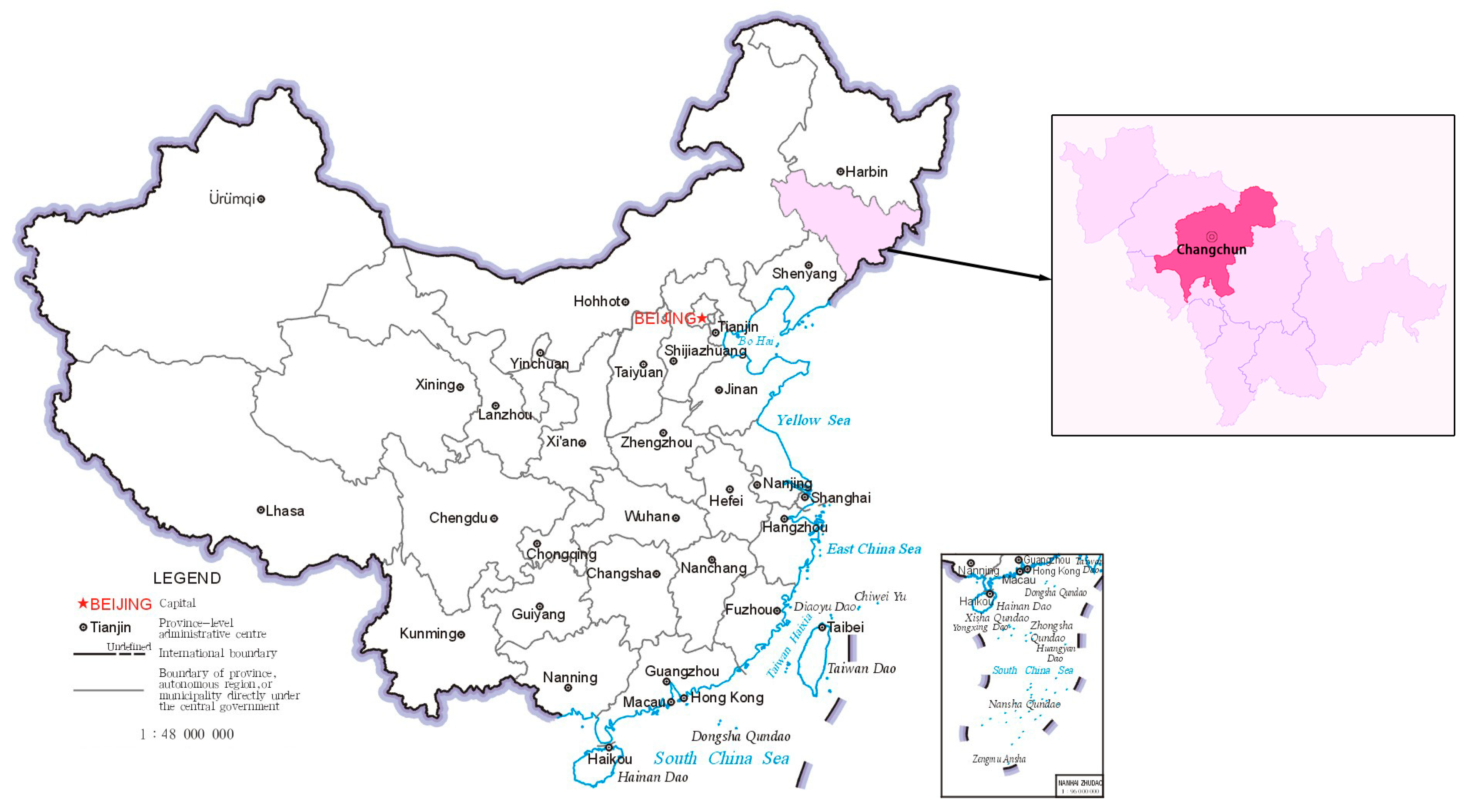
Changchun City is located in the middle of Jilin Province in northeast China (Figure 1), and its geographical position is advantageous, being east of Jilin City, west of Songyuan City, south of Siping City, and north of Songhua River. Its geographical coordinates span 43°05′ N to 45°15′ N in latitude and 124°18′ E to 127°02′ E in longitude, with a total area of approximately 20,571 km². The terrain of Changchun City is mostly flat, with some mountainous areas in the eastern and southern regions. Overall, the elevation gradually decreases from the southeast to the northwest. In terms of climate, Changchun City experiences a typical temperate continental monsoon climate, with distinct seasons. Winters are cold and long, summers are hot and humid, and spring and autumn are brief and subject to frequent weather changes. Sunshine is sufficient, but the lack of precipitation in winter leads to dry air, and the air quality in winter is susceptible to adverse meteorological conditions, especially industrial emissions and vehicle exhaust.

In terms of industrial development, Changchun, as China’s “automobile city”, has the automobile manufacturing industry as its leading industry, which has driven the rapid development of related industries. However, the increase in industrial production and energy consumption has also brought pressure on the air quality, especially during the winter heating period. Because precipitation is low, pollutants in the air cannot easily diffuse and settle, which has an adverse impact on air quality [24].

3.2. Data Sources

The data sources used in this study encompass three main aspects: (1) Air pollutant concentration data obtained from the China Air Quality Online Monitoring Platform, collected hourly from 10 national control monitoring stations located in the main urban area and surrounding regions of Changchun City. The platform aggregates these hourly measurements, including PM_2.5 and PM₁₀ concentrations, into publicly available daily averages; (2) Meteorological data provided by the Changchun Meteorological Station, comprising hourly measurements of temperature, humidity, wind speed, and other meteorological variables from the Changchun National Reference Climate Station (station ID 54161) and four auxiliary stations. Daily averages were calculated using arithmetic means; (3) Energy price data sourced from financial terminals, which include daily updates on natural gas and fuel gas prices. The research data encompassed three dimensions: air pollutant concentrations (e.g., CO, NO₂, PM_2.5, PM₁₀, SO₂, O₃), meteorological variables (e.g., average, maximum, and minimum pressure and temperature, average and minimum relative humidity, daily precipitation, maximum wind speed), and energy prices (e.g., natural gas and gas).

The Air Quality Index (AQI) is calculated using a piecewise linear interpolation method based on the Individual Air Quality Index (IAQI) of each pollutant. The specific steps are as follows: first, the concentration values of each pollutant are obtained from monitoring data; second, the IAQI for each pollutant is calculated using Formula (1):

$$IAQ{I}_P={\displaystyle \frac{IAQ{I}_{Hi}-IAQ{I}_{Lo}}{B{P}_{Hi}-B{P}_{Lo}}}\times \left(C_P-B{P}_{Lo}\right)+IAQ{I}_{Lo}$$

(1)

The IAQI for each pollutant is calculated, where $C_P$ represents the measured concentration, $B{P}_{Hi}$ and $B{P}_{Lo}$ are the concentration breakpoints adjacent to $C_P$ in the reference table, and $IAQ{I}_{Hi}$ and $IAQ{I}_{Lo}$ are the corresponding index values at these breakpoints. Finally, the maximum IAQI among all pollutants is taken as the current AQI value, and the primary pollutant as well as any pollutants exceeding the standard are identified. Meteorological changes directly or indirectly influence the generation, dispersion, and removal of pollutants, affecting air quality. Additionally, energy prices exhibit a negative correlation with energy consumption [25]. Therefore, this study integrates air pollutant concentrations, meteorological conditions, and energy prices to analyze the air quality index (AQI), thereby offering significant practical applications.

3.3. Data Preprocessing

The Air Quality Index (AQI), also known as the Air Quality Index or Air Pollution Index, is an indicator that measures air quality and assesses its impact on human health, ecosystems, and the environment. The AQI transforms complex air quality data into a single value that is easy to understand by taking into account the concentration of multiple air pollutants. To evaluate the performance of the model, the dataset was divided into a training set and a testing set, with 80% allocated for training and 20% for testing. This division allows for the effective utilization of the data for model training while retaining sufficient data to assess the model’s generalization ability. A random splitting method was employed during the division process, and a fixed random seed was set to ensure the reproducibility of the results.

Through a comprehensive analysis of air quality and meteorological data, data preprocessing, including the elimination of outliers, processing of missing values, and descriptive statistical analysis, was performed to ensure the accuracy and completeness of the data. Any correlation between the variables was then revealed, and key features were identified through exploratory data analysis. The LightGBM and SHAP methods were used for feature engineering to construct feature data and label data and to increase the dimensions of the data. First, outliers and missing values were processed. In this study, outliers are defined as data points that deviate significantly from the majority of the observations in the dataset. These values exhibit noticeable numerical differences compared with other data points and do not conform to the general distribution patterns of the dataset. Statistical methods were employed to identify and handle these outliers to ensure data quality and enhance the reliability of the model. After data processing, outliers were identified and removed using a standard deviation-based method, where data points beyond the range of μ ± 10σ were defined as outliers. A total of six extreme outliers were excluded. For missing values in continuous variables (with a missing rate below 5%), median imputation was applied. The cleaned dataset more accurately reflects the true conditions and provides a reliable foundation for subsequent analyses. A descriptive statistical analysis was performed to understand the basic characteristics and distribution of the data. Exploratory data analysis (EDA) was conducted based on data preprocessing, including correlation and feature importance analyses. Feature engineering constructs features and labels. In this process, we not only retain key information from the original dataset but also add dimensions to the data. These methods not only enrich the information of the dataset but also help to improve the prediction ability and generalization ability of the model.

According to

Table 1. Descriptive statistical analysis.

	Mean Value	Maximum Value	Minimum Value	Standard Deviation	Variance
PM2.5	42.95	433.00	0.00	40.84	1667.81
PM10	73.27	465.00	0.00	51.66	2668.79
SO2	18.62	146.00	0.00	21.75	472.92
NO2	34.40	113.00	0.00	13.99	195.66
CO	0.80	3.19	0.00	0.36	0.13
O3	54.90	184.00	0.00	26.99	728.53
Natural gas price	3.39	3.70	2.94	0.30	0.09
Gas price	6.57	13.69	3.62	1.74	3.03
Mean pressure	986.88	1011.20	956.30	8.74	76.39
Maximum pressure	989.55	1012.90	967.10	8.84	78.11
Minimum pressure	984.04	1009.60	951.60	8.77	76.92
Mean air temperature	7.06	29.90	26.10	13.98	195.40
Maximum air temperature	11.84	35.70	24.10	14.23	202.46
Minimum air temperature	2.54	28.70	30.30	14.09	198.50
Mean relative humidity	61.55	100.00	14.00	18.07	326.68
Minimum relative humidity	40.17	99.00	5.00	17.96	322.41
Daily precipitation	1.93	99.90	0.00	6.80	46.24

, the mean values of PM_2.5 and PM₁₀ are 42.95 and 73.27 respectively, while the mean values of SO₂ and NO₂ are lower at 18.62% and 34.40%. Energy prices are relatively stable, with less volatility in the natural gas and gas prices. The data for barometric pressure, temperature, and humidity showed some volatility, with an average barometric pressure of 986.88 hPa, an average temperature of 7.06°C, and an average relative humidity of 61.55 % RH. Precipitation and wind speed data show maximum daily precipitation and maximum wind speeds of 99.90 mm/day and 25.20 m/s, respectively. The average Air Quality Index (AQI) was 71.16, indicating a moderate level of air quality overall during the observation period.

3.4. Correlation Analysis

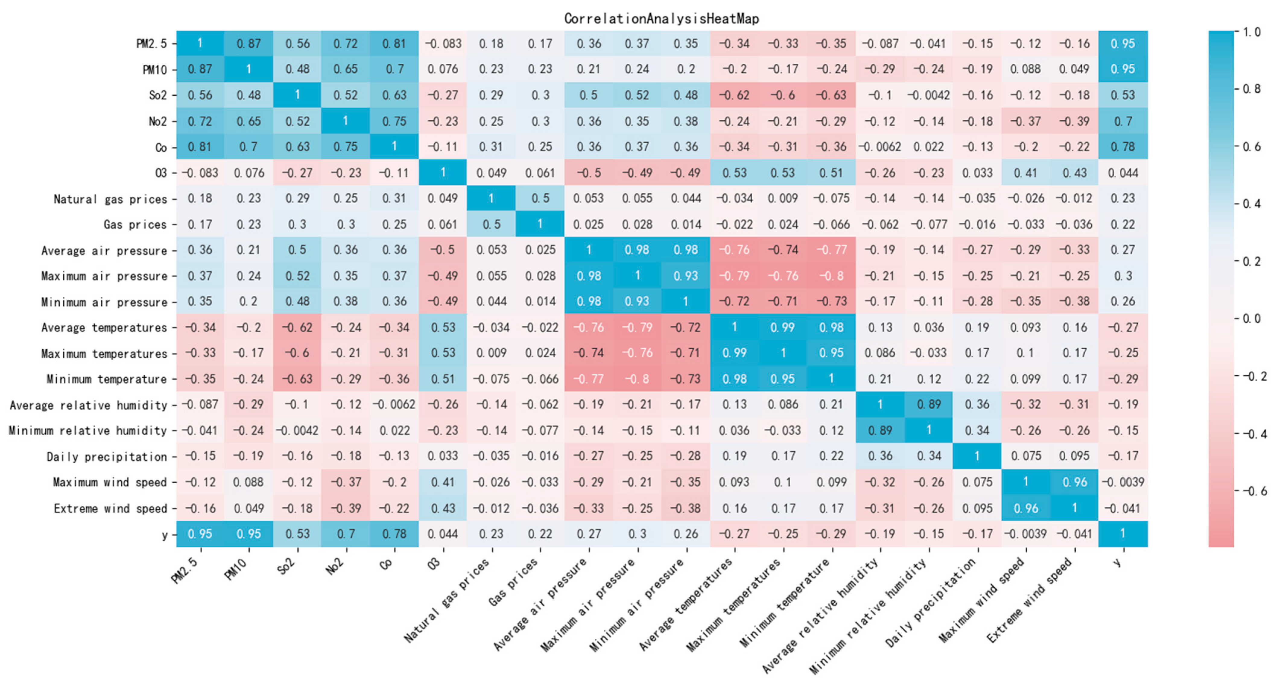
The Pearson correlation coefficient was used to analyze the correlation between variables, and its value range was [−1, 1]. The greater the absolute value of the coefficient, the stronger the correlation between the variables, and vice versa. The AQI may be affected by other pollutants or weather conditions, and there is a certain correlation. Therefore, a prediction model was built using the influencing factors related to the AQI, and the correlation between air quality (AQI) and other pollutants and meteorological data was analyzed in Python (3.8.19). Figure 2 shows the thermal map of the correlation analysis. The analysis results indicate that the AQI is correlated with other influencing factors in the dataset. Specifically, the correlation coefficients between the AQI and PM_2.5, PM₁₀, SO₂, NO₂, and CO were 0.95, 0.95, 0.53, 0.7, and 0.78, respectively. All the coefficients had absolute values greater than 0.5, indicating a significant relationship between the AQI and these factors. Additionally, the AQI is notably influenced by temperature and atmospheric pressure.

3.5. Methods

3.5.1. Pelican Optimization Algorithm

The Pelican Optimization Algorithm (POA), introduced by Trojovský and Mohammad Dehghani in 2022 [26], is a novel nature-inspired optimization method. This algorithm is based on the predatory behavior of pelicans, which mimics their hunting strategies and movements. The algorithm iteratively refines candidate solutions by simulating two main phases of the hunting process: approaching the prey (exploration phase) and gliding over the water surface to capture the target (exploitation phase).

The mathematical formulation for initializing the pelican population is as follows:

$${\mathrm{x}}_{\mathrm{i},\mathrm{j}}={\mathrm{l}}_{\mathrm{j}}+\mathrm{r}\mathrm{a}\mathrm{n}\mathrm{d}\cdot \left({\mathrm{u}}_{\mathrm{j}}-{\mathrm{l}}_{\mathrm{j}}\right),\mathrm{i}=1,2,\dots ,\mathrm{N},\mathrm{j}=1,2,\dots ,\mathrm{m}$$

(2)

In Equation (2), ${\mathrm{x}}_{\mathrm{i},\mathrm{j}}$ represents the position of the i-th pelican in the j-th dimension; N denotes the population size of the pelican group; m refers to the dimensionality of the problem being solved; rand is a random number within the range [0, 1]; and ${\mathrm{u}}_{\mathrm{j}}$ and ${\mathrm{l}}_{\mathrm{j}}$ are the upper and lower boundaries of the j-th dimension for the problem, respectively.

In the Pelican Optimization Algorithm, the objective function evaluates the fitness values of the pelicans to solve the problem. The objective values of the pelican population are represented as a vector of fitness values as follows:

$${\left.\mathrm{F}=\left[\begin{array}{c}{\mathrm{F}}_1\\ ⋮\\ {\mathrm{F}}_i\\ ⋮\\ {\mathrm{F}}_{\mathrm{N}}\end{array}\right.\right]}_{\mathrm{N}\times 1}={\left[\begin{array}{c}\mathrm{F}\left({\mathrm{X}}_1\right)\\ ⋮\\ \mathrm{F}\left({\mathrm{X}}_{\mathrm{i}}\right)\\ ⋮\\ \mathrm{F}\left({\mathrm{X}}_{\mathrm{N}}\right)\end{array}\right]}_{\mathrm{N}\times 1}$$

(3)

In Equation (3), F is the objective function vector of the pelican population, and ${\mathrm{F}}_i$ is the objective function value of the i-th pelican.

Phase 1: Approaching the prey (exploration phase).

In the first phase, the pelican identifies the prey’s position and moves toward the designated area. To model this strategy, the POA algorithm is designed to effectively scan the search space, thereby enhancing its exploration capabilities across different regions. A key feature of the POA is that the position of the prey is randomly generated within the search space, which strengthens the exploration ability of the algorithm for precise search problems. The following presents the mathematical modeling of this concept and the strategy for approaching prey:

$${\mathrm{x}}_{\mathrm{i},\mathrm{j}}^{{\mathrm{P}}_1}=\left\{\begin{array}{l}{\mathrm{x}}_{\mathrm{i},\mathrm{j}}+\mathrm{rand}·\left({\mathrm{p}}_{\mathrm{j}}-\mathrm{I}·{\mathrm{x}}_{\mathrm{i},\mathrm{j}}\right), {\mathrm{F}}_{\mathrm{p}}<{\mathrm{F}}_{\mathrm{i}}\\ {\mathrm{x}}_{\mathrm{i},\mathrm{j}}+\mathrm{rand}·\left({\mathrm{x}}_{\mathrm{i},\mathrm{j}}-{\mathrm{p}}_{\mathrm{j}}\right), \mathrm{else}\end{array}\right.$$

(4)

In Equation (4), ${\mathrm{x}}_{\mathrm{i},\mathrm{j}}^{{\mathrm{P}}_1}$ represents the position of the i-th pelican in the j-th dimension after the update in the first phase; rand is a random number within the range [0, 1]; I is a random integer that takes a value of either 1 or 2; ${\mathrm{p}}_{\mathrm{j}}$ represents the position of the prey in the j-th dimension; and ${\mathrm{F}}_{\mathrm{p}}$ is the objective function value of the prey.

In the POA algorithm, when the objective function value improves at a given position, the pelican accepts the new position. These updates, known as valid updates, ensure that the algorithm avoids suboptimal areas. This process can be mathematically expressed as

$${\mathrm{X}}_{\mathrm{i}}=\left\{\begin{array}{cc}{\mathrm{X}}_{\mathrm{i}}^{{\mathrm{P}}_1},& {\mathrm{F}}_{\mathrm{i}}^{{\mathrm{P}}_1}<{\mathrm{F}}_{\mathrm{i}}\\ {\mathrm{X}}_{\mathrm{i}},& \mathrm{else}\end{array}\right.$$

(5)

In Equation (5), ${\mathrm{X}}_{\mathrm{i}}^{{\mathrm{P}}_1}$ represents the new position of the i-th pelican, and ${\mathrm{F}}_{\mathrm{i}}^{{\mathrm{P}}_1}$ is the objective function value corresponding to the new position ${\mathrm{X}}_{\mathrm{i}}^{{\mathrm{P}}_1}$ of the i-th pelican after the update in the first phase.

Phase 2: Surface flight (development phase).

In the second phase, when pelicans fly over the water surface, they spread their wings, push the fish toward the surface, and capture their prey in their throat pouch. This flying strategy allows pelicans to capture more fish within the attack zone. By modeling this behavior, the POA algorithm can converge more effectively to optimal positions within the hunting region, thereby enhancing its local search and exploitation capabilities. From a mathematical perspective, the algorithm examines the area surrounding the pelican’s position to improve the convergence to superior locations. The pelican’s behavior during the hunting process can be mathematically modeled as follows:

$${\mathrm{x}}_{\mathrm{i},\mathrm{j}}^{{\mathrm{P}}_2}={\mathrm{x}}_{\mathrm{i},\mathrm{j}}+\mathrm{R}·\left(1-{\displaystyle \frac{\mathrm{t}}{\mathrm{T}}}\right)·\left(2·\mathrm{r}\mathrm{a}\mathrm{n}\mathrm{d}-1\right)·{\mathrm{x}}_{\mathrm{i},\mathrm{j}}$$

(6)

In Equation (6), ${\mathrm{x}}_{\mathrm{i},\mathrm{j}}^{{\mathrm{P}}_2}$ represents the position of the i-th pelican in the j-th dimension after the update in the second phase; rand is a random number within the range [0, 1]; R is a random integer that takes a value of either 0 or 2; t is the current iteration number; and T is the maximum number of iterations.

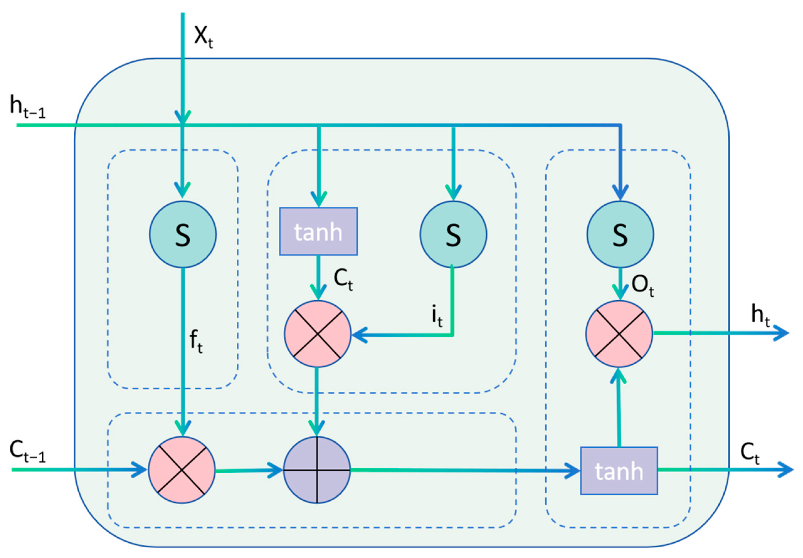
3.5.2. LSTM

Long Short-Term Memory (LSTM) is an improved mode of the Recurrent Neural Network (RNN), which was proposed by Hochreiter et al. [27] in 1997 and adopts LSTM. The layer replaces the traditional hidden layer and achieves the effective screening and long-term memory of information by introducing three types of “gate” structures: input, output and forgetting gates. The LSTM structure is shown in Figure 3.

The calculation formula is as follows:

$$f_t=\sigma \left(w_f·\left[h_{t-1},x_t\right]+b_f\right)$$

(7)

$$i_t=\sigma \left(w_i·\left[h_{t-1},x_t\right]+b_i\right)$$

(8)

$$c_t^{\prime }=\tanh \left(w_c·\left[h_{t-1},x_t\right]+b_c\right)$$

(9)

$$c_t=f_t\times C_{t-1}+i_t\times c_t^{\prime }$$

(10)

$$o_t=\sigma \left(w_0·\left[h_{t-1},x_t\right]+b_0\right)$$

(11)

$$h_t=o_t\times \tanh \left(c_t\right)$$

(12)

In Equations (7)–(12), $f_t$ represents the forgetting threshold; $i_t$ indicates the input threshold; $c_t^{\prime }$ indicates the cell state at the previous moment; $c_t$ indicates the current cell state; $o_t$ indicates the output threshold; $h_t$ represents the unit output at time t; $x_t$ represents the input at time t; $\sigma$ denotes the sigmoid function; tanh stands for hyperbolic tangent function; $w_f,w_i,w_c,\mathrm{a}\mathrm{n}\mathrm{d} w_0$ represent the weight matrices for the forget gate, input gate, cell state, and output gate respectively;$\mathrm{a}\mathrm{n}\mathrm{d} b_f,b_i,b_c,\mathrm{a}\mathrm{n}\mathrm{d} b_o$ represent the bias vectors for the forget gate, input gate, cell state, and output gate, respectively.

3.5.3. Convolutional Neural Networks

A CNN, as proposed by Lecun et al., has the characteristics of automatic data acquisition and strong adaptability [28]. A CNN is composed of convolutional, pooling, and fully connected layers, and the structure of a CNN is shown in Figure 4.

Convolutional layer: The convolutional layer is a fundamental component of Convolutional Neural Networks (CNNs), and the convolutional operation is performed through a convolutional check to extract the features of the input data.

Pooling layer: A pooling layer can reduce the space size of the feature map and reduce the model complexity.

Fully connected layer: The fully connected layer is a traditional neural network layer which can flatten the features extracted by the previous convolutional and pooling layers and perform classification or regression through the fully connected layer.

3.5.4. Construction of the Pelican Algorithm to Optimize the CNN-LSTM Model

In the field of air quality prediction, the spatiotemporal distribution of pollutant concentrations is influenced by multiple factors, including meteorological conditions, geographical environment, and human activities. To address these complexities, we have adopted a hybrid architecture combining Convolutional Neural Networks (CNNs) and Long Short-Term Memory (LSTM) networks. CNNs excel at extracting local spatial features, providing critical spatial information for prediction, while LSTM networks effectively capture long-term temporal dependencies, accommodating the seasonality, periodicity, and long-term trends in air quality data. Air quality data exhibit not only spatial correlations but also pronounced seasonality, periodicity, and long-term trends. For instance, air quality is periodically affected by meteorological factors such as wind direction, wind speed, and precipitation. The gating mechanism of LSTM enables it to effectively memorize these long-term temporal characteristics, thereby better predicting future air quality trends.

Compared with other hybrid architectures (such as CNN-GRU or RNN-LSTM), the CNN-LSTM architecture has significant advantages. Although GRUs (Gated Recurrent Units) and RNNs (Recurrent Neural Networks) can also be used for time-series modeling, the gating mechanism of LSTM allows it to more effectively memorize and utilize long-term temporal features, which is crucial for capturing the seasonality and periodicity in air quality data. CNN-LSTM strikes a better balance between computational complexity and prediction accuracy when dealing with complex spatiotemporal data. Compared with CNN-GRU, it is more robust in handling long-term dependencies, especially when the data contain noise or missing values. Compared with RNN-LSTM, it more efficiently captures the spatial correlations of pollutant concentrations through convolutional layers, thereby enhancing prediction accuracy. Overall, CNN-LSTM ensures high prediction accuracy while reducing computational costs, making it an efficient and practical solution for air quality prediction.

In this study, a hybrid model combining the Pelican Optimization Algorithm (POA), a Convolutional Neural Network (CNN), and a Long Short-term Memory (LSTM) network is proposed. The model design includes the following key modules (Figure 5): By using the Pelican Optimization Algorithm (POA) to optimize hyperparameters—such as the learning rate (ranging from 0.001 to 0.2) and the number of neurons in the LSTM layer (ranging from 49 to 60)—the approach achieves a globally optimal selection, reducing the complexity of manual tuning. First, the input data is processed through a CNN to extract local features and to capture spatial correlations. Then, a Flatten layer is used to convert the features into a one-dimensional vector, which is fed into the LSTM layer to capture temporal dependencies. Finally, the feature vector is passed through a fully connected layer for nonlinear combination and regression prediction, yielding the final output.

In addition, an Early Stopping mechanism is introduced into the model training, which can automatically stop the training by monitoring the loss of the verification set, which avoids overfitting and improves the training efficiency. In combination with the dynamic learning-rate-adjustment strategy, the model uses a higher learning rate during the early stages of training to accelerate convergence and dynamically reduces the learning rate in the later stage to improve the accuracy. The Pelican Optimization Algorithm runs through the entire process of hyperparameter selection model training and optimizes the balance between global searching and local development by simulating pelican predation behavior, further improving the stability and generalization ability of the model. The experimental results indicate that the model has excellent prediction ability in complex air quality prediction tasks and can efficiently capture the spatiotemporal characteristics and global trends in multidimensional data while maintaining high computational efficiency, providing a new way to solve similar time-series prediction problems.

3.5.5. Evaluation Indicators

The experiments were conducted on a Windows 11 operating system, utilizing an AMD Ryzen 7 4800U processor, 16 GB DDR4 RAM (15.4 GB available), and integrated AMD Radeon Graphics. The development environment comprised Python 3.8.19, with the key libraries including TensorFlow 2.4.1 for the neural network construction and training, NumPy 1.19.5 for mathematical computations, Pandas 1.1.5 for data processing, scikit-learn 0.24.1 for the machine learning tasks, and Matplotlib 3.3.4 for result visualization. All operations were executed via Python scripting.

To compare the predictive performance of each model, the mean absolute error, root mean squared error, and r-squared and explained variance were selected to assess the predictive performance of each model. The MAE measures the average absolute difference between the model’s predicted and actual values, which reflects the magnitude of the prediction error. This reflects the degree to which the model’s prediction deviates from the true value. The RMSE measures the square root of the squared mean of the forecast error and reflects the overall size of the forecast error. R is used to measure the proportion of change in the explanatory variables of the model. That is, it represents how much of the population variance the model can explain. The EVS is a direct reflection of the model’s ability to explain the variance of real data and has a value range of [0, 1].

$$RMSE=\sqrt{{\displaystyle \frac{1}{n}}\sum _{i=1}^n({\widehat{y}}_i-y_i{)}^2}$$

(13)

$$MAE={\displaystyle \frac{1}{n}}\sum _{i=1}^n|{\widehat{y}}_i-y_i|$$

(14)

$$R^2=1-{\displaystyle \frac{\sum _{i=1}^n(y_i-{\widehat{y}}_i{)}^2}{\sum _{i=1}^n\left(y_i-{\tilde{y}}_i\right)}}$$

(15)

$$EVS=1-{\displaystyle \frac{\sum _{i=1}^n(y_i-{\widehat{y}}_i{)}^2}{\sum _{i=1}^n(y_i-\overline{y}{)}^2}}$$

(16)

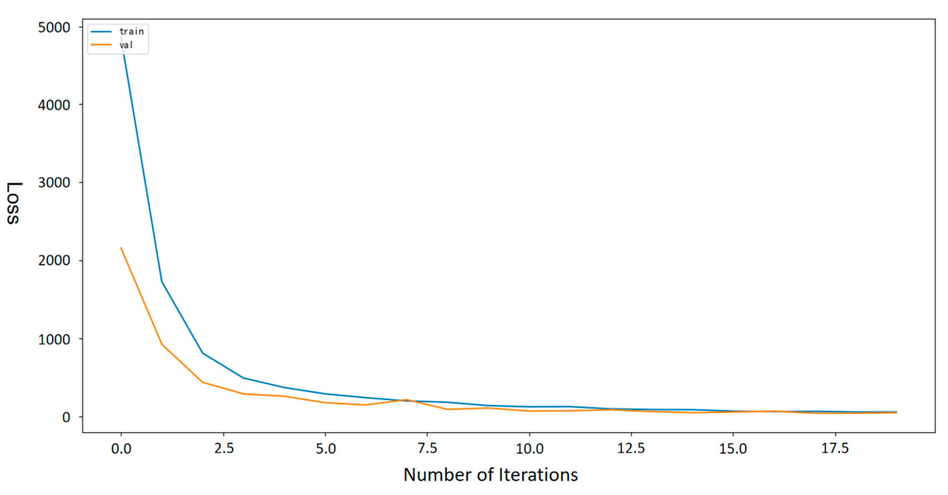
Figure 6 shows the process in which the Pelican Optimization Algorithm is applied to the LSTM recurrent neural network regression model, and how the model loss value gradually decreases with an increase in the number of iterations. The vertical axis represents the loss value, which ranges from 0 to 5000, whereas the horizontal axis denotes the number of iterations, which ranges from 0 to 20. The curve in the figure shows that with an increase in the number of iterations, the loss value gradually decreases from a high value, indicating that the model performance gradually improves during the optimization process until it becomes stable.

4. Results

4.1. Feature Importance Analysis

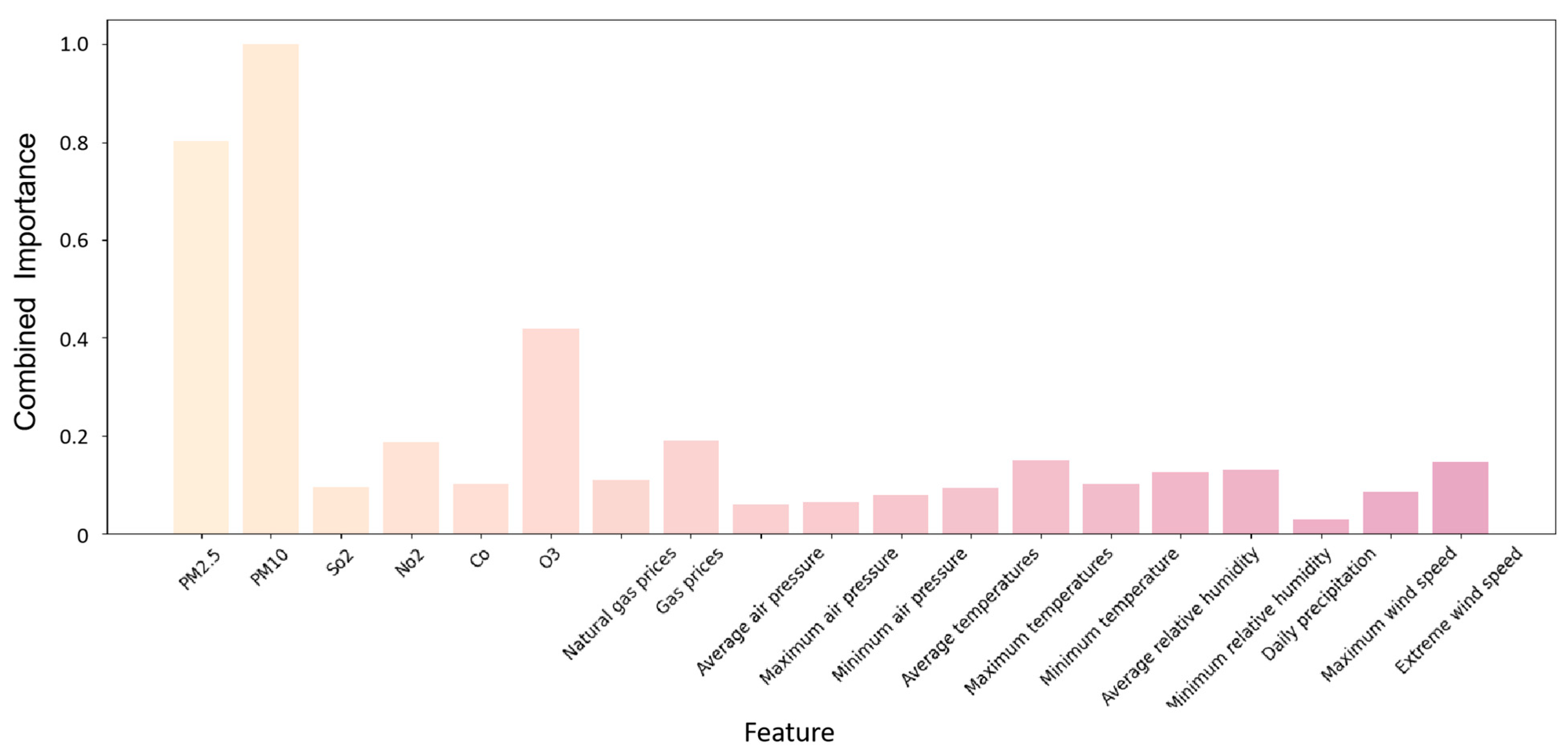
Through the combined analysis of LightGBM and SHAP, we were able to identify the key factors that affect air quality and to understand how these factors work together in different situations. LightGBM provides a fast and efficient way to assess the importance of features in large amounts of data, whereas SHAP provides the specific contributions of each feature to model predictions. The advantage of this combined approach is that it combines the features of both models to provide a more comprehensive and in-depth analysis of the feature importance.

As shown in Figure 7, traditional air pollutants such as PM_2.5, PM₁₀, NO₂, and O₃ have high Eigen importance scores, which is consistent with our existing understanding of the role that these pollutants play in air quality. These pollutants often originate from industrial emissions, transportation, and combustion processes and have significant negative effects on human health and the environment.

In addition to gaseous pollutants, meteorological factors play a crucial role in air quality modeling. Meteorological conditions not only influence the diffusion and chemical reactions of gaseous pollutants but also govern their deposition. For example, high temperatures and intense sunlight are key factors in ozone formation, providing the necessary energy and radiation for photochemical reactions. Changes in atmospheric pressure affect air density and mobility, thereby regulating pollutant diffusion. In high-pressure regions, the subsiding air suppresses vertical pollutant diffusion. Elevated temperatures promote atmospheric instability, facilitate vertical pollutant diffusion, and accelerate chemical reactions involving gases such as ozone. Fluctuations in relative humidity alter the hygroscopic properties of particulate matter, thereby affecting its physical characteristics, residence time, and settling rate in the atmosphere. Precipitation is a natural cleansing mechanism that removes particulate matter and other soluble pollutants through wet deposition. Finally, wind speed and direction determine the rate and trajectory of the pollutant dispersion. Higher wind speeds can rapidly transport pollutants over greater distances, whereas wind direction dictates the movement of pollutants. The combined effects of these meteorological factors are essential for the predictive accuracy of air quality models.

4.2. Comparative Experiment

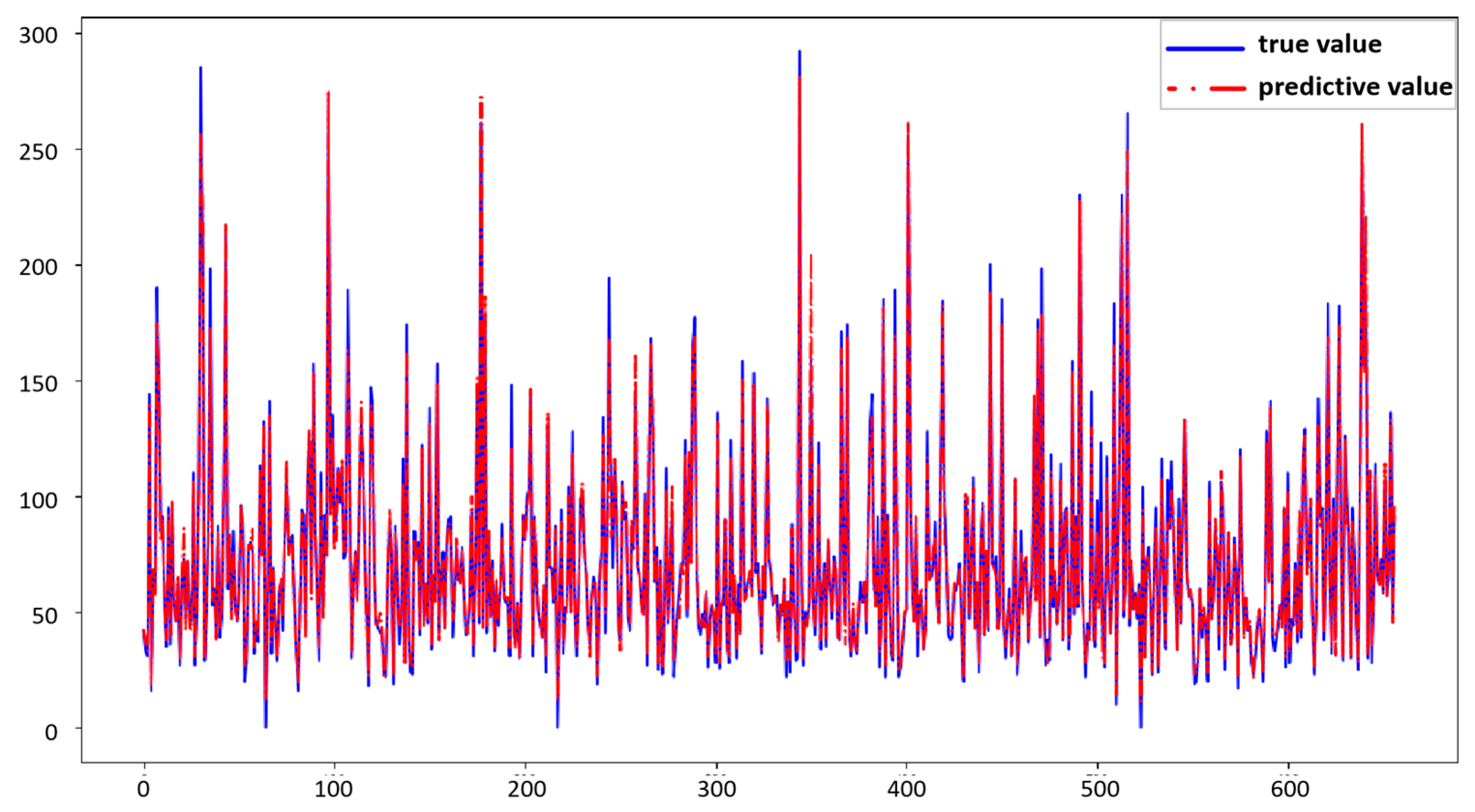
The root mean squared error (RMSE) and mean absolute error (MAE) of this model are 6.7421 and 4.2767, respectively. These two indicators are lower than those of the conventional forecasting model, indicating that this model has the smallest error in forecasting and shows high forecasting accuracy. Second, the explanatory variance score (EVS) and coefficient of determination (R²) of the model are 0.9877 and 0.9871, respectively, indicating that the model is better able to capture patterns and trends in the data as well as more effectively explain the variability of the data. The prediction results are shown in Figure 8.

As shown in

Table 2. Experimental results of the model comparisons.

Prediction Model	RMSE	MAE	EVS	R2
KNN	8.2540	5.3647	0.9657	0.9656
Linear regression	7.8889	5.2459	0.9685	0.9685
Support vector machine	7.9094	5.1347	0.9688	0.9684
Gradient lifting	8.2952	5.6748	0.9653	0.9653
This model	6.7421	4.2767	0.9877	0.9871

and Figure 9, The RMSE of this model is 6.7421, which is the lowest among the comparison models, indicating that its prediction error is the best, and the gap with the true value is the smallest. The R² is 0.9871, which is also the highest in the comparison model, indicating that this model can explain most of the variation in the dependent variables, and the fitting effect is very good.

In summary, the RMSE is concerned with the size of the prediction error, whereas R² is concerned with the model’s ability to explain the variation in the data. Both are important indicators for evaluating the performance of the model, and this model shows the best performance for these two indicators, indicating that it is the best in terms of forecasting accuracy and explanatory ability.

The analysis results show that this model not only has excellent performance in reducing prediction errors, but it also has obvious advantages in the explanatory ability and fitting effect of the model.

4.3. Ablation Experiment

The results in

Table 3. Comparison results of ablation experiments.

Prediction Model	RMSE	MAE	EVS	R2
CNN	9.1970	6.3533	0.9578	0.9573
POA + CNN	8.2987	5.6869	0.9656	0.9652
PSO + CNN	8.2593	5.7486	0.9721	0.9655
LSTM	16.5617	11.7183	0.8628	0.8616
PSO + LSTM	14.2162	5.4714	0.9028	0.8979
POA + LSTM	18.4559	7.5992	0.8305	0.8280
PSO + CNN + LSTM	10.0766	7.0704	0.9671	0.9488

and Figure 10 show that there are significant differences in the performance of various models, and the introduction of optimization algorithms improves the prediction performance of the models. The underlying models (CNN and LSTM) showed significant differences. The lower error of the CNN and the better performances of the interpretive difference (EVS) and coefficient of determination (R²) indicate that the CNN has a strong fitting ability when processing this dataset. The error of the LSTM model is obviously higher, especially in the root mean squared error (RMSE) and the mean absolute error (MAE), which are much higher than those of the other models, indicating that LSTM does not fully exploit its advantages in this task.

After the introduction of the optimization algorithm, both the POA and PSO significantly improved the performance of the model. The optimization of CNN by both the POA and PSO significantly reduced the error of the model and improved its explanatory ability. The two optimizations are very close, but PSO is slightly better than the POA, showing lower errors and higher EVS and R² values.

For the optimization of LSTM, PSO also significantly reduces the error of LSTM and improves the model performance, whereas the optimization effect of the POA is relatively poor and fails to achieve the ideal effect. Combining the performance of the POA and PSO on LSTM shows that LSTM is not as good as the CNN model in this task.

Although the combination model of PSO-CNN-LSTM introduces the fusion of three technologies, it does not show significant improvement and the size of the error increases. This may be because the characteristics of the different models are not fully coordinated, resulting in the advantages of the fusion model not being reflected.

This model has the highest performance, with the lowest error and highest explanatory power, indicating that innovations in the architecture or optimization algorithm enable it to achieve the best predictive performance over all the other models. This shows that a reasonable design and optimization of the model structure can greatly improve the prediction effect.

5. Discussion

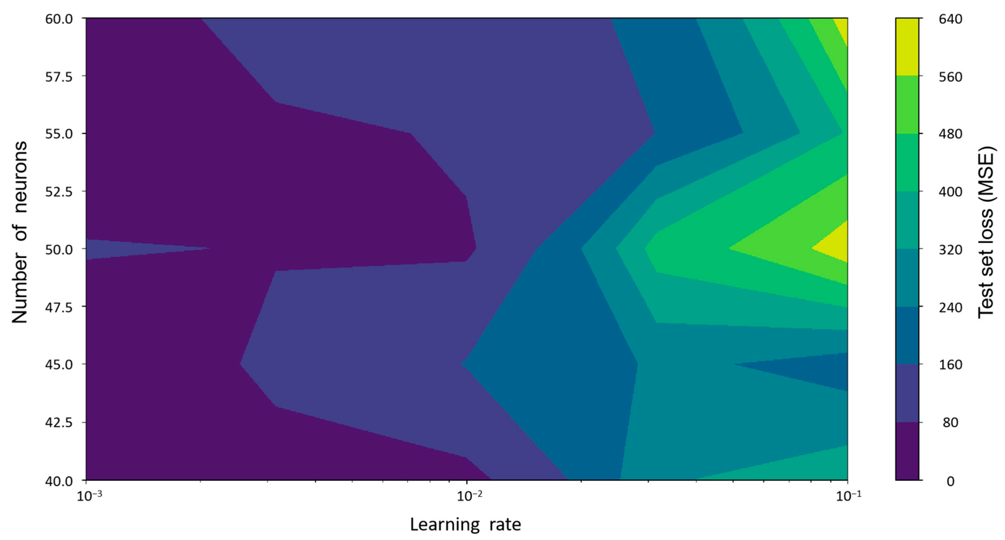
To verify the robustness of the proposed model and the rationality of the hyperparameter selection, a sensitivity analysis was conducted on the number of neurons and the learning rate. Figure 11 illustrates the model’s loss values (mean squared error, MSE) on the test set under different combinations of hyperparameters. The horizontal axis represents the learning rate (on a logarithmic scale), while the vertical axis shows the number of hidden layer neurons in the LSTM, and the color intensity indicates the magnitude of the test loss for each combination.

The results reveal a clear fluctuation trend in the test loss as the hyperparameters vary, indicating that the model’s performance is highly sensitive to these two parameters. When the learning rate is low (e.g., 0.001), the overall error is smaller, and the model performs best when the number of neurons is 45 or 50. This suggests that the model is more stable and has stronger generalization ability within this range. As the learning rate increases, the test error rises significantly, with the worst performance observed at a learning rate of 0.1, indicating that an excessively high learning rate can lead to unstable training.

This sensitivity analysis further confirms the significant impact of hyperparameter selection on model performance and provides a theoretical basis for subsequent model optimization and parameter tuning. By selecting configurations with a lower learning rate and an appropriate number of neurons, the prediction accuracy and model robustness can be effectively improved.

To further validate the robustness and generalization capability of the proposed model, multiple experiments were conducted under different training-to-testing data splits. The results demonstrate that the model consistently achieves high predictive accuracy, regardless of whether the training data proportion is 80%, 70%, 60%, or 50%. Additionally, we supplemented the evaluation with computational efficiency metrics, including total runtime and peak memory usage. The detailed results are presented in

Table 4. Model performance and resource consumption under different training/testing splits.

Test Set: Training Set	EVS	R2	Total Runtime	Peak Memory Usage
20%: 80%	0.9877	0.9871	17 min 22.76 s	49.71 MB
30%: 70%	0.9837	0.9832	17 min 26.68 s	60.33 MB
40%: 60%	0.9772	0.9748	15 min 6.94 s	56.99 MB
50%: 50%	0.9761	0.9725	13 min 3.76 s	61.66 MB

.

As shown in Table 4, the model maintains consistently high predictive performance across various data partitioning strategies while also demonstrating good computational efficiency in terms of runtime and memory usage. This indicates that the proposed model not only excels in accuracy but also possesses strong adaptability to limited computational resources, making it suitable for practical applications where resource constraints exist.

The model not only considers the time-series characteristics of the data but also pays special attention to the nonlinear characteristics of the data. The Pelican Optimization Algorithm was chosen to optimize the model. The POA does not require derivative information of the objective function, and it is suitable for nonlinear, non-convex, multimodal optimization problems that cannot be easily solved by traditional algorithms. Therefore, compared with the single and other combined models, this model has obvious advantages in prediction accuracy, and the prediction error is also significantly reduced.

This study has some limitations. The prediction of air quality is a complex problem involving seasonal and spatiotemporal differences. Future studies can further explore how to incorporate seasonal and spatial factors into the model to improve the accuracy and robustness of the prediction [29,30,31]. Although this study made some progress in air quality prediction, there is still room for improvement. Future studies can further optimize the model to improve the accuracy and applicability of the forecast by considering seasonal and other potential influencing factors.

6. Conclusions

This study proposes on optimized CNN-LSTM air quality prediction model based on the POA algorithm. The experimental results show the following:

(1) In ensuring the prediction accuracy, the model makes full use of the global search capability of the POA, the local feature-extraction capability of the CNN, and the time-dependent capture capability of the LSTM, providing an efficient solution for complex regression tasks and time-series prediction.

(2) An Early stopping mechanism is introduced in the training of this model, which can automatically stop the training in the event of loss to avoid overfitting and to improve the training efficiency. In the later stages, the precision was optimized gradually, which significantly improved the prediction performance and stability of the model.

(3) Although this study demonstrates the outstanding potential and value of the Pelican Optimization Algorithm (POA)-driven CNN-LSTM fusion model in forecasting tasks, there is still room for improvement in computational resource efficiency, model architecture simplification, and cross-domain applicability. Future research should focus on optimizing the model design, exploring spatiotemporal correlation and seasonality, in greater depth, expanding the applicability of the model in multidimensional data analysis, and promoting its widespread use in air quality prediction and other time-series applications.

(4) Improving the ability to predict air quality not only helps to scientifically formulate environmental strategies for agriculture and animal husbandry but also optimizes the sustainability of the ecosystem and reduces the impact of environmental pollution on agricultural production and livestock health, thus providing significant ecological and economic benefits. The POA-optimized CNN-LSTM fusion model proposed in this study provides a novel, efficient and robust solution for complex time-series prediction. Through continuous research and optimization, this method will play an increasingly important role in air quality monitoring and environmental management, providing solid technical support for achieving the goals of green development and a sustainable environment.