Influence of Building Envelope Modeling Parameters on Energy Simulation Results

Abstract

This study investigates the influence of input values for building energy model parameters on simulation results, with the aim of improving the reliability and sustainability of energy performance assessments. Dynamic simulations were conducted in TRNSYS for three theoretical multi-residential buildings, varying parameters such as referent model dimensions, infiltration rates, envelope thermophysical properties, and interior thermal capacitance. The case study, based in Slovenia, demonstrates that glazing-related parameters, particularly the solar heat gain coefficient (g-value), exert the most significant influence—reducing the g-value from 0.62 to 0.22 decreased simulated heating (q_H,nd) and cooling (q_C,nd) demands by 25% and 95%, respectively. In contrast, referent dimensions for modeled floor area proved least influential. For Building III (BSF = 0.36), dimensional variations altered results by less than ±1%, whereas, for Building I (BSF = 0.62), variations reached up to ±20%. In general, lower shape factors yield more robust energy models that are less sensitive to input deviations. These findings are critical for promoting resource-efficient simulation practices and ensuring that energy modeling contributes effectively to sustainable building design. Understanding which inputs warrant detailed attention supports more targeted and meaningful simulation workflows, enabling more accurate and impactful strategies for building energy efficiency and long-term environmental performance.

1. Introduction

Energy production, distribution, and use remain at the center of global environmental, technical, and economic concerns. The building sector alone accounts for approximately 40% of the total final energy use and 36% of greenhouse gas (GHG) emissions within the European Union. Operational energy, primarily from heating, cooling, and ventilation systems, contributes significantly to this, representing about 60% of the sector’s energy demand. In households, this share rises further, with 70% of final energy used for space heating and an additional 14% for sanitary hot water preparation [1,2]. Increasing the energy efficiency of buildings is, therefore, a central strategy in mitigating climate change.

In response, the European Union has enacted several directives, most notably the Energy Performance of Buildings Directive (EPBD), including its original form (2002/91/EC) and subsequent recasts (2010/31/EU and 2018/844/EU). These directives define minimum energy performance requirements, promote building renovations, and support the integration of renewable energy sources. Importantly, the EPBD encourages the application of standardized energy performance assessments, typically grounded in dynamic building energy simulation (BES) models.

BES plays a crucial role in achieving optimized building design and post-construction operation, thereby contributing to sustainable development goals. These simulations support informed decision-making by enabling the evaluation of energy-saving measures, control strategies, and building envelope designs prior to implementation.

However, the simulation process can be complex and computationally demanding, especially when considering a wide range of variables and configurations. A clear understanding of how modeling parameters affect simulation outcomes is essential for effectively allocating computational and human resources. This understanding is not only critical for the accurate prediction of energy use but also for optimizing energy efficiency and sustainability in both new and existing buildings.

BES tools are based on physics-driven (law-driven) models that simulate the response of the building to various environmental and operational conditions, incorporating thermophysical envelope properties, occupancy profiles, internal loads, and HVAC system behavior. Alternatively, data-driven models, including black-box (e.g., artificial neural networks) and grey-box models, have gained traction due to their potential for rapid calibration and reduced input requirements. However, law-driven models remain dominant in regulatory, certification, and design contexts due to their transparency and comprehensive treatment of thermal phenomena. A detailed discussion of grey-box methodologies and applications is provided by Li et al. [3].

Dynamic BES models, as opposed to quasi-steady-state approaches, offer high temporal resolution and can account for hourly variations in weather, occupancy, and internal loads. Crawley et al. [4] conducted an extensive comparison of major simulation tools, including TRNSYS, EnergyPlus, IDA ICE, and others, emphasizing differences in modeling depth, required inputs, and computational effort. Dynamic simulation is particularly beneficial when modeling the impact of design decisions on HVAC sizing, control strategies, and thermal comfort. Ferrero et al. [5], Pacheco et al. [6], and Zakula et al. [7] provide useful overviews of how different simulation programs and methods can be applied at various stages of building design.

However, the reliability of building simulation models depends on many factors, including the physical accuracy of the model, user input quality, and model calibration. Validation studies comparing simulation tools with experimental measurements, such as test-box experiments and monitored buildings, have provided benchmarks for tool performance and have highlighted sources of uncertainty and deviation [8,9,10]. Recent cross-comparative studies show that the accuracy and consistency between various simulation engines (such as EnergyPlus, IDA ICE, and TRNSYS) can differ significantly depending on boundary conditions, timestep settings, and assumed parameters [11,12].

These findings underline the need for a critical assessment of tool selection and for sensitivity analysis when dealing with input assumptions that significantly affect performance predictions. These issues have elevated the role of uncertainty and sensitivity analysis in building energy modeling. Sensitivity analysis, in particular, serves as a systematic method to assess the relative influence of model input parameters on simulation outcomes. It has been widely used for optimizing design parameters [13], evaluating the robustness of retrofit strategies [14], and informing model calibration efforts [15].

Several studies have expanded on this by exploring the robustness of simulation results and the impact of modeling assumptions. Hensen and Lamberts [16] provided foundational insights into simulation tool applications and limitations. Wang et al. [17] reviewed quantitative energy assessment frameworks, while Dermentzis et al. [18] evaluated monthly auditing in renovation contexts. Nageler et al. [19] and Mangi et al. [20] emphasized the validation of models under real experimental conditions, using test boxes and thermally activated systems. Calleja Rodríguez et al. [21] introduced macroparameter sensitivity approaches that reduce model complexity without compromising reliability. Connolly et al. [22] and Gelesz et al. [23] demonstrated how tool selection and input definition influence performance predictions in cases of renewable integration and façade design. Mazzeo et al. [24] compared tool outputs using test boxes with and without PCMs, helping to benchmark simulation accuracy across engines.

While many sensitivity studies focus on variables like occupancy or weather, which are difficult to control, other parameters such as envelope properties, glazing characteristics, and geometric assumptions are within the modeler’s control. These design-dependent inputs often lack precise specification early in the design process or in retrofitting existing buildings.

This study contributes to this discussion by analyzing how different modeling assumptions related to envelope geometry and thermophysical input values influence simulation results for typical multi-residential buildings. A set of simplified geometric models is used to isolate the effects of parameters such as building shape factor (BSF), glazing properties, infiltration rate, and thermal capacitance. Dynamic simulations are conducted in TRNSYS to evaluate the sensitivity of simulated heating and cooling demands to selected parameter variations.

The objective of this study is to evaluate the sensitivity of building energy simulation results to different configurations of envelope modeling parameters within dynamic simulation software. By doing so, the paper aims to provide both researchers and building professionals with practical guidance on which parameters are most influential and how simulation resources should be allocated to yield the most meaningful outcomes. This insight supports the broader goal of enhancing the efficiency, transparency, and sustainability of building energy performance assessments.

2. Materials and Methods

This study investigates the influence of input assumptions related to building envelope and geometric modeling on energy simulation results. The analysis was conducted using the dynamic simulation software TRNSYS 17, which is based on the Transfer Function Method (TFM) and enables hourly simulations of building thermal behavior under transient conditions.

The focus of this research is on assessing how envelope-related input parameters—such as thermophysical properties of walls and windows, infiltration rates, thermal capacitance of interior space, and modeled floor area—affect the simulated annual energy needed for heating (q_H,nd) and cooling (q_C,nd) per unit floor area of conditioned space. The heating and cooling systems are assumed to be ideal (unlimited capacity, perfect control), and no internal gains from occupancy, lighting, or equipment are modeled. This allows for the isolation of envelope-driven effects, without confounding influences from operational or user-related variables.

The goal is not to simulate realistic energy use scenarios, but rather to explore the sensitivity of energy demand results to uncertain or variable input assumptions in the envelope modeling process.

Simulations were performed using the Typical Meteorological Year (TMY) for Ljubljana, Slovenia, compiled by the Slovenian Environmental Agency using the adapted Sandia method. The local climate is classified as Cfb (temperate oceanic climate) according to the Köppen–Geiger classification. Weather file data include hourly values for dry-bulb temperature, solar radiation (global and diffuse), wind speed, and humidity.

TRNSYS solves hourly energy balance equations that account for radiative, convective, and conductive heat transfers. The envelope was modeled using the Transfer Function Method, per Mitalas and Arseneault [25]. Heating and cooling capacities were assumed unlimited, ensuring that setpoint temperatures were always met (ideal control). The model excludes ventilation (mechanical or natural), internal heat gains, or latent loads, focusing solely on sensible heating and cooling needs under standard boundary conditions.

Energy balance equations in the simulation model include net radiative heat transfer ${\dot{q}}_{r,s,o}$ and ${\dot{q}}_{r,s,i}$ absorbed radiation heat fluxes S_s,o and S_s,i, conduction heat fluxes ${\dot{q}}_{s,o}$ and ${\dot{q}}_{s,i}$, and convection heat fluxes ${\dot{q}}_{c,s,o}$ and ${\dot{q}}_{c,s,i}$. A detailed description of the TRNSYS mathematical model is available at [25].

The three case-study buildings are modeled as unoccupied spaces during the simulation period, with no internal heat gains from occupants or equipment. All simulations assume a conditioned floor area defined either by internal, external, or middle wall surfaces (depending on the test case). The boundary conditions are aligned with the Slovenian Rulebook on Efficient Use of Energy in Buildings [26], and heating/cooling setpoints are set to 20 °C for heating and 26 °C for cooling, consistent with EN ISO 7730 [27].

Three theoretical building models of identical height (9 m, three stories) and varying footprints were used to evaluate how building shape factor (BSF) affects sensitivity to modeling assumptions. The BSF is defined as the ratio of the external envelope area to the conditioned floor area. Buildings I, II, and III have footprints of 10 × 10 m, 20 × 20 m, and 30 × 30 m, with corresponding BSFs of 0.62, 0.42, and 0.36, respectively. All buildings maintain a 20% window-to-floor ratio and the same thermophysical properties.

A total of 189 simulations were carried out, with a controlled variation of the following parameters:

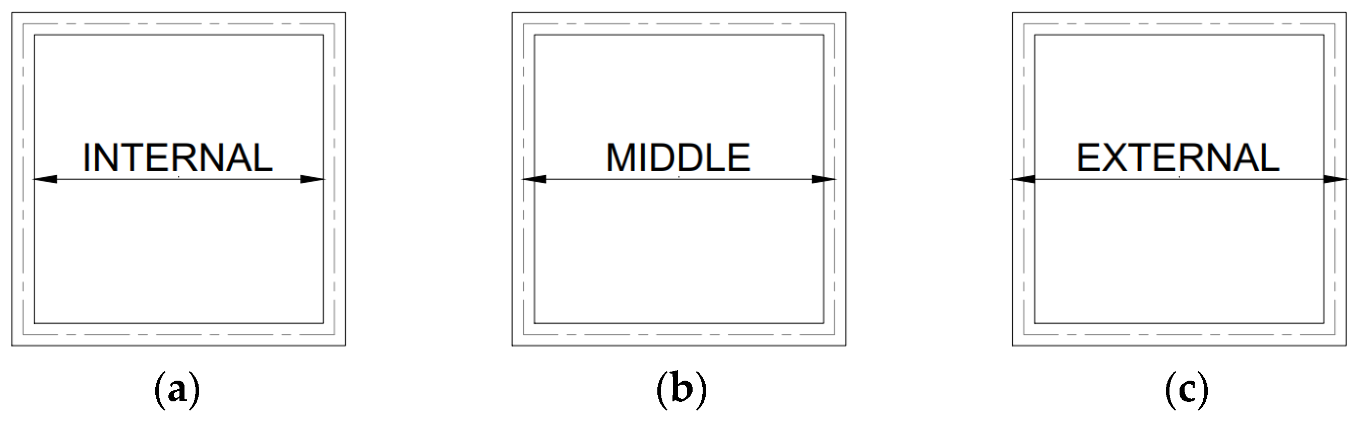
• Geometric reference for floor area modeling (internal, middle, or external wall surface);
• Infiltration modeled using either air changes per hour (ACH) or fixed airflow rate (m³/h);
• Window parameters: frame U-value, frame factor (FF), glazing U-value, and solar heat gain coefficient (g-value);
• Wall U-values and thermal bridge linear transmittance (ψ-values);
• Thermal mass of interior space, with added wood furniture occupying 1% and 2% of internal volume.

Each variation isolates the effect of a single parameter while all others remain fixed at baseline values.

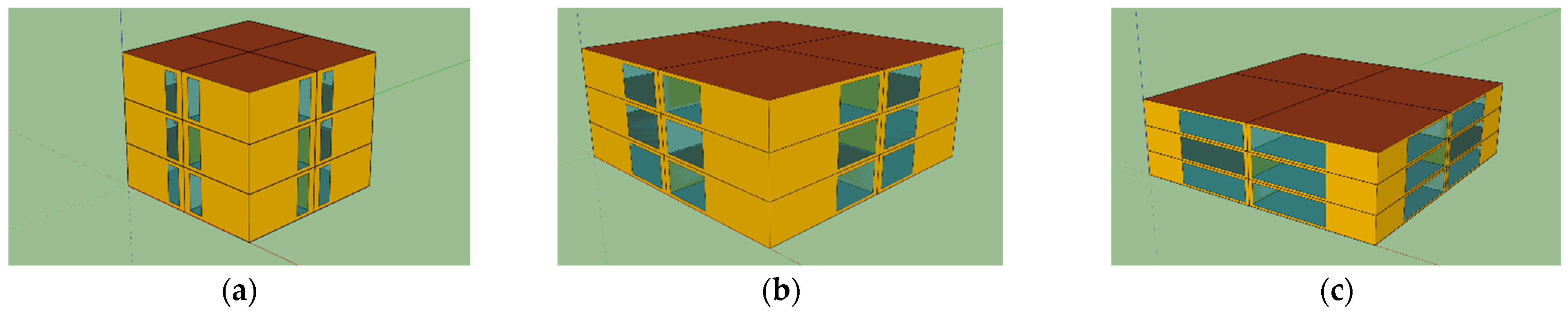
2.1. Baseline Building Description

The three baseline buildings used in this study represent typical residential construction in Slovenia over the past several decades. All buildings are theoretical models located in Ljubljana and differ only in their footprint dimensions: 10 × 10 m, 20 × 20 m, and 30 × 30 m, each with a height of 9 m distributed over three stories (Figure 1). These variations allow for an evaluation of how the building shape factor (BSF) influences the sensitivity of energy simulation results to variations in envelope-related input parameters. The BSFs for the three buildings are 0.62, 0.42, and 0.36, respectively (

Table 1. Baseline building sizes.

Label	Footprint	Height	BSF
Building I	10 m × 10 m	9 m (three stories)	0.62
Building II	20 m × 20 m	9 m (three stories)	0.42
Building III	30 m × 30 m	9 m (three stories)	0.36

).

The thermophysical properties of the envelope components for the baseline buildings were selected to reflect characteristics of modern Slovenian multi-family residential buildings constructed within the last 30 years (i.e., from the early 1990s to 2021), prior to the full implementation of the Nearly Zero Energy Building (NZEB) standard. This reflects a typical condition found in the existing housing stock built under the evolving energy efficiency requirements set by national regulations.

As of 2021, all new buildings in Slovenia are required to meet NZEB criteria, as defined by the “Pures” Rulebook and its amendments [26], which align with the Energy Performance of Buildings Directive (EPBD) recast requirements [1]. Although the buildings modeled in this study are not NZEB per se, their thermophysical properties correspond to common practices used prior to the current NZEB mandate. This includes wall U-values around 0.18 W/m²K, roof U-values below 0.30 W/m²K, and modern glazing systems with low-emissivity coatings.

For further contextualization, studies such as Šijanec Zavrl et al. [28] and Dolinar et al. [29] provide detailed analysis of the Slovenian building stock and trends in envelope construction practices, confirming that the modeled thermophysical characteristics correspond well with prevalent construction from the 1990s through 2020.

The same envelope specifications and internal conditions (e.g., infiltration rate of 0.5 ACH; setpoint temperatures of 20 °C for heating and 26 °C for cooling) are applied to all three models. Detailed material compositions of the walls, roof, and floor are presented in

Table 2. Thermophysical properties of exterior wall layers (total U-value = 0.176 W/m²K; thickness 0.52 m).

	Thickness (m)	Density (kg/m3)	Conductivity (W/mK)	Specific Heat (kJ/kgK)
Mortar1900	0.020	1900	3.564	1.05
Hollow Brick	0.290	1400	2.196	0.92
Mineral Wool	0.200	140	0.144	1.03
Mortar_ext	0.005	1550	2.520	1.05
Mortar Silikat	0.005	1550	2.520	1.05

,

Table 3. Slab floor on grade.

	Thickness (m)	Density (kg/m3)	Conductivity (W/mK)	Specific Heat (kJ/kgK)
Parquet	0.020	700	0.756	1.67
Concrete2200	0.060	2200	5.436	0.96
XPS	0.100	35	0.137	1.50
Hydro insulation	0.010	1100	0.684	1.46

and

Table 4. Roof.

	Thickness (m)	Density (kg/m3)	Conductivity (W/mK)	Specific Heat (kJ/kgK)
Mortar1900	0.020	1900	3.564	1.05
Concrete2400	0.120	2200	5.436	0.96
Concrete2200	0.050	2200	7.344	0.96
Hydro insulation	0.010	1100	0.684	1.46
XPS	0.220	35	0.137	1.50
Gravel	0.080	1700	2.916	0.84

.

2.2. Variation of Referent Dimensions for Modeled Floor Area

According to various building energy modeling standards, including the National Energy Code of Canada for Buildings (2017) [30] and industry practice guidelines (e.g., Scott West et al. [31]), the modeled floor area (MFA) must typically fall within a specified range of the gross floor area indicated in architectural drawings. As a result, building geometry is often derived from the external dimensions of the envelope (i.e., between the outside surfaces of exterior walls). However, alternative approaches based on internal dimensions or the midline of the wall (Figure 2) are also used in practice, depending on local conventions and data availability. This variation is acknowledged in EN ISO 52016-1:2017, EN ISO 13790, and EN ISO 52000-1, which emphasize that floor area definitions should align with national calculation methodologies. These geometric assumptions directly affect the modeled air volume and envelope area, thereby influencing simulated infiltration rates and thermal loads. In this study, we explicitly examine the impact of these differing reference geometries by testing all three options—internal, external, and midline—across a range of building sizes.

Obviously, MFA is directly correlated with the modeled volume of air inside a thermal zone since internal air volume equals MFA times the height from floor to ceiling.

Furthermore, infiltration rate is typically modeled using one of two input parameters: (a) number of air changes per hour (ACH) or (b) infiltration airflow rate (m³/h). If the first approach is used, the simulated infiltration rate is correlated to the modeled air volume of a thermal zone and consequently to MFA.

To evaluate the effect of model parameters defining MFA and infiltration on simulated energy performance, a set of simulations is provided for different combinations of those parameters (

Table 5. Building I: MFA dimensions and infiltration rates.

	Modeled Dimensions	MFA [m2]	Internal Volume [m3]	ACH	Volume Flow m3/h	Simulation ID
Building I	Internal	300.00	900.00	0.50	450	1.1 (baseline)
	Middle	332.01	996.03	0.50	498	1.2
				0.45	450	1.3
	External	365.65	1096.93	0.50	548	1.4
				0.41	450	1.5
Building II	Internal	1200	3600	0.50	1800	2.1 (baseline)
	Middle	1263	3790	0.50	1895	2.2
				0.47	1800	2.3
	External	1328	3984	0.50	1992	2.4
				0.45	1800	2.5
Building III	Internal	2700	8100	0.50	4050	3.1 (baseline)
	Middle	2794	8383	0.50	4192	3.2
				0.48	4050	3.3
	External	2890	8671	0.50	4336	3.4
				0.47	4050	3.5

). For simulations with ID x.1, x.2, x.4, the infiltration is modeled as 0.5 ACH, while, for the simulations with ID x.3, x.5, the infiltration is modeled using an airflow rate that corresponds to the baseline case and is independent of which referent dimensions were used.

2.3. Variations of Building Envelope Modeling Parameters

Building envelope has a critical impact on building energy performance, which is recognized by building energy standards and is the topic of numerous research efforts. Nevertheless, when creating a building simulation model, exact specifications for building envelope elements, including external walls and windows, are usually not available. This refers to exact U-values for exterior walls, as well as windows’ parameters, including frame U-value, frame to window area, and glazing properties. Therefore, the model parameters for walls and windows are usually defined based on assumptions, using typical values for thermal transmittance (U-value) and solar heat gain coefficient (g-value). A set of simulations has been provided by varying parameters for external walls: U-value, window frame U-value, F_F, glazing U-value and g-value, and windows to floor ratio, as presented in

Table 6. Modeling parameters for external walls and windows.

		Building I	Building II	Building III
Envelope Parameter	Value	Simulation ID	Simulation ID	Simulation ID
Window to floor ratio	20%	1.1 (baseline)	2.1 (baseline)	3.1 (baseline)
	25%	1.6	2.6	3.6
	30%	1.7	2.7	3.7
Windows frame U-value	1.5 W/m2K	1.1 (baseline)	2.1 (baseline)	3.1 (baseline)
	1.2 W/m2K	1.8	2.8	3.8
	0.9 W/m2K	1.9	2.9	3.9
Window frame factor	30%	1.1	2.1	3.1
	25%	1.10	2.10	3.10
	20%	1.11	2.11	3.11
Glazing U-value (g = 0.62)	1.10 W/m2K	1.1 (baseline)	2.1 (baseline)	3.1 (baseline)
	0.88 W/m2K	1.12	2.12	3.12
	0.62 W/m2K	1.13	2.13	3.13
Glazing g-value (U = 1.1 W/m2K)	0.62	1.1 (baseline)	2.1 (baseline)	3.1 (baseline)
	0.42	1.14	2.14	3.14
	0.22	1.15	2.15	3.15
External wall U-value	0.176 W/m2K	1.1 (baseline)	2.1 (baseline)	3.1 (baseline)
	0.140 W/m2K	1.16	2.16	3.16
	0.315 W/m2K	1.17	2.17	3.17

. In each simulation, only one parameter is changed compared to the baseline.

2.4. Variation of Thermal Bridging

The effect of thermal bridges on building energy performance is significant, yet sometimes partially overlooked [32,33]. In TRNSYS dynamic simulation, the impact of thermal bridges is considered by providing the value for linear or point thermal transmittances (ψ) of thermal bridges within the building envelope, which is in line with the methodology defining thermal bridging provided by the European Standard EN ISO 14683. The simulation set includes three variations with ψ = 0 W/mK (baseline), ψ = 0.05 W/mK, and ψ = 0.10 W/mK (

Table 7. Modeling parameters for thermal bridges.

		Building I	Building II	Building III
Envelope Parameter	Value	Simulation ID	Simulation ID	Simulation ID
ψ	0 W/mK	1.1 (baseline)	2.1 (baseline)	3.1 (baseline)
	0.05 W/mK	1.18	2.18	3.18
	0.10 W/mK	1.19	2.19	3.19

). The length of thermal bridges was 23 m (simulations 1.18 and 1.19), 43 m (simulations 2.18 and 2.19), and 63 m (simulations 3.18 and 3.19) per thermal zone.

2.5. Variation of Interior Space Thermophysical Properties

Furniture/indoor thermal mass has an impact on building energy flows and can affect energy efficiency [34]. The baseline energy models have been created with an interior space that contains only air, and no additional thermal mass. Additional simulations have been provided to assess how including the thermal capacity of furniture affects simulated building energy performance. In addition to the baseline condition, a simulation including wood furniture that occupies 1% and 2% of internal building volume respectively was provided (

Table 8. Modeling parameters for thermal capacitance.

		Building I	Building II	Building III
Parameter	Value	Simulation ID	Simulation ID	Simulation ID
Thermal capacitance	air	1.1 (baseline)	2.1 (baseline)	3.1 (baseline)
	1% wood	1.20	2.20	3.20
	2% wood	1.21	2.21	3.21

). Wood density is 600 kg/m³, and the specific heat of wood is 2.09 kJ/kgK.

3. Results and Discussion

The TRNSYS dynamic simulations quantified the annual energy required for heating (q_H,nd) and cooling (q_C,nd) per unit floor area for three theoretical buildings in Slovenia, highlighting the impact of varying building envelope parameters. The results focus on deviations from baseline models caused by changes in inputs such as glazing g-value, thermal bridging, infiltration, and external wall U-value. These variations revealed significant differences in energy performance, particularly for buildings with higher building shape factors (BSF), where envelope parameters exert greater influence.

A notable finding was the increase in cooling energy demand resulting from the improved thermal insulation of envelope elements—a counterintuitive outcome driven by solar gains. During cooling periods, solar heat gains often dominate, particularly when outdoor temperatures fall below the 26 °C setpoint, leading to a reversal of heat flux from indoors to outdoors. Enhanced insulation reduces this passive cooling effect, trapping more heat indoors and thereby increasing mechanical cooling needs (EN ISO 14683, 2017). This underscores the complex interplay of envelope properties in dynamic simulations, emphasizing the need for careful parameter specification to optimize energy performance [3].

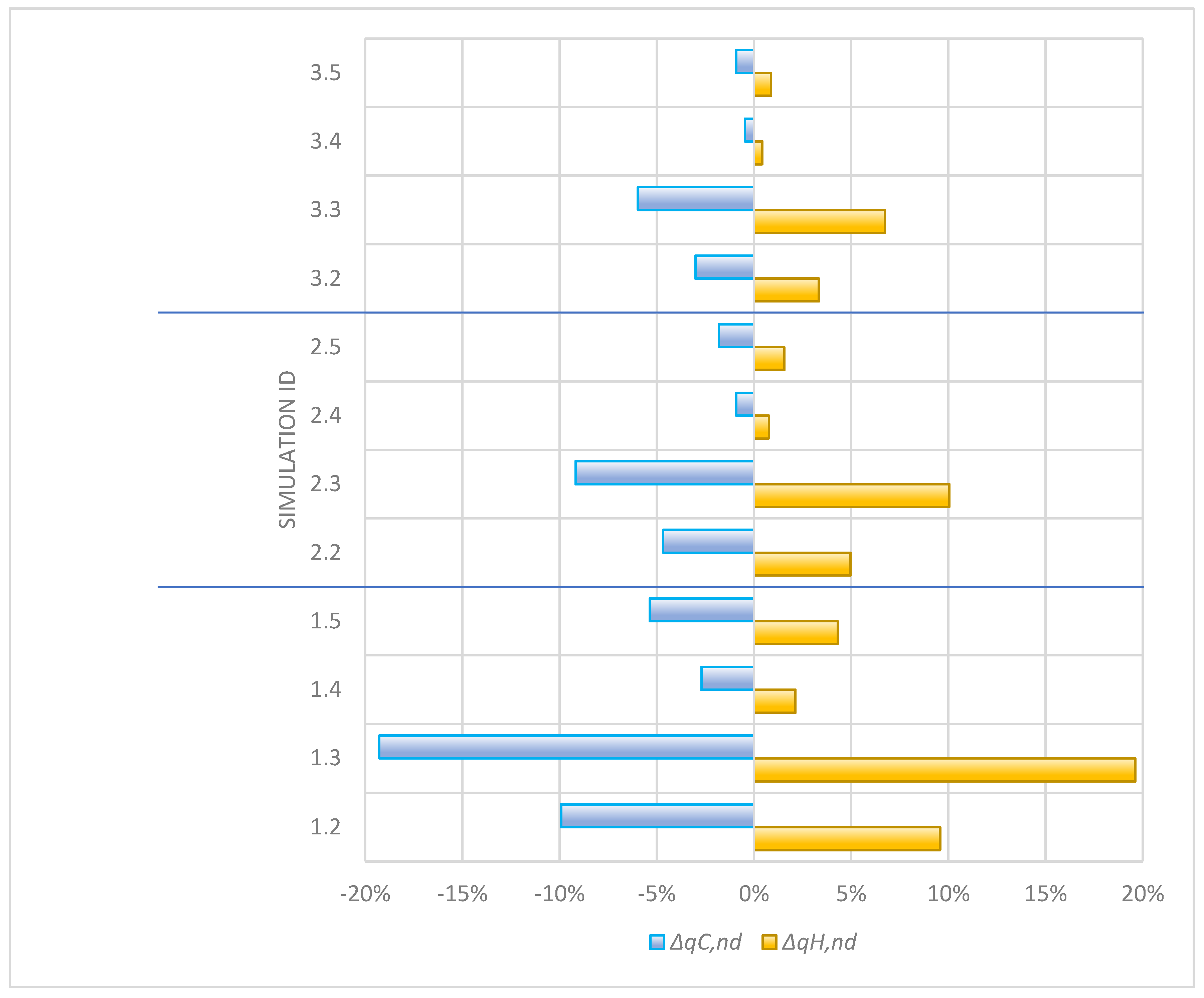
3.1. Simulation Results for Variation of Referent Dimensions

Results presented in

Table 9. Building I simulation results for varying MFA and infiltration rate parameters.

Building I (10 × 10)
Simulation ID	Description	qH,nd [kWh/m2]	Δ qH,nd	qC,nd [kWh/m2]	Δ qC,nd
1.1	internal; 0.5 ACH (450 m3/h)	52.49	Baseline	6.48	Baseline
1.2	middle; 0.5 ACH (498 m3/h)	57.51	9.57%	5.84	−9.92%
1.3	external; 0.5 ACH (548 m3/h)	62.78	19.61%	5.23	−19.28%
1.4	middle; 450 m3/h	53.60	2.13%	6.31	−2.70%
1.5	external; 450 m3/h	54.75	4.31%	6.14	−5.37%

,

Table 10. Building II simulation results for varying MFA and infiltration rate parameters.

Building II (20 × 20)
Simulation ID	Description	qH,nd [kWh/m2]	Δ qH,nd	qC,nd [kWh/m2]	Δ qC,nd
2.1	internal; 0.5 ACH (1800 m3/h)	45.51	Baseline	7.47	Baseline
2.2	middle; 0.5 ACH (1895 m3/h)	47.76	4.96%	7.12	−4.67%
2.3	external; 0.5 ACH (1992 m3/h)	50.08	10.05%	6.78	−9.18%
2.4	middle; 1800 m3/h	45.86	0.77%	7.40	−0.91%
2.5	external; 1800 m3/h	46.21	1.56%	7.33	−1.81%

and

Table 11. Building III simulation results for varying MFA and infiltration rate parameters.

Building III (30 × 30)
Simulation ID	Description	qH,nd [kWh/m2]	Δ qH,nd	qC,nd [kWh/m2]	Δ qC,nd
3.1	internal; 0.5 ACH (4050 m3/h)	43.28	Baseline	7.80	Baseline
3.2	middle; 0.5 ACH (4192 m3/h)	44.72	3.34%	7.57	−3.01%
3.3	external; 0.5 ACH (4336 m3/h)	46.19	6.74%	7.33	−5.98%
3.4	middle; 4050 m3/h	43.46	0.43%	7.77	−0.46%
3.5	external; 4050 m3/h	43.65	0.87%	7.73	−0.92%

show that selection of referent MFA dimensions (internal, middle, or external) can have a significant impact on energy performance assessment for buildings with smaller footprints and higher BSF (i.e., Building I). When external dimensions are considered as referent, with infiltration modeled as 0.5 ACH, for Building I, which has the highest BSF of 0.62, the difference in simulated energy needed for heating and cooling is 19.61% and −19.28%, respectively, compared to the baseline case, for which internal dimensions are considered as a referent. As the building shape factor decreases, the influence of the choice of referent dimensions diminishes. For Building II (BSF = 0.42), Δ q_H,nd and Δ q_C,nd are 10.05% and −9.18%, respectively, while, for Building III, with the lowest BSF (0.36), Δ q_H,nd = 6.74% and Δ q_C,nd = 5.98%.

Furthermore, if infiltration is modeled using the flow rate parameter instead of ACH, then the difference in simulated energy performance is additionally reduced.

Ultimately, for Building III, with BSF = 0.36, if infiltration is modeled using the airflow rate parameter, the choice of referent dimensions becomes almost irrelevant, as the difference between simulated energy performance compared to the baseline is less than 1%.

The correlations between variations of parameters for MFA and infiltration and the relative difference in simulated energy performance are clearly illustrated in Figure 3.

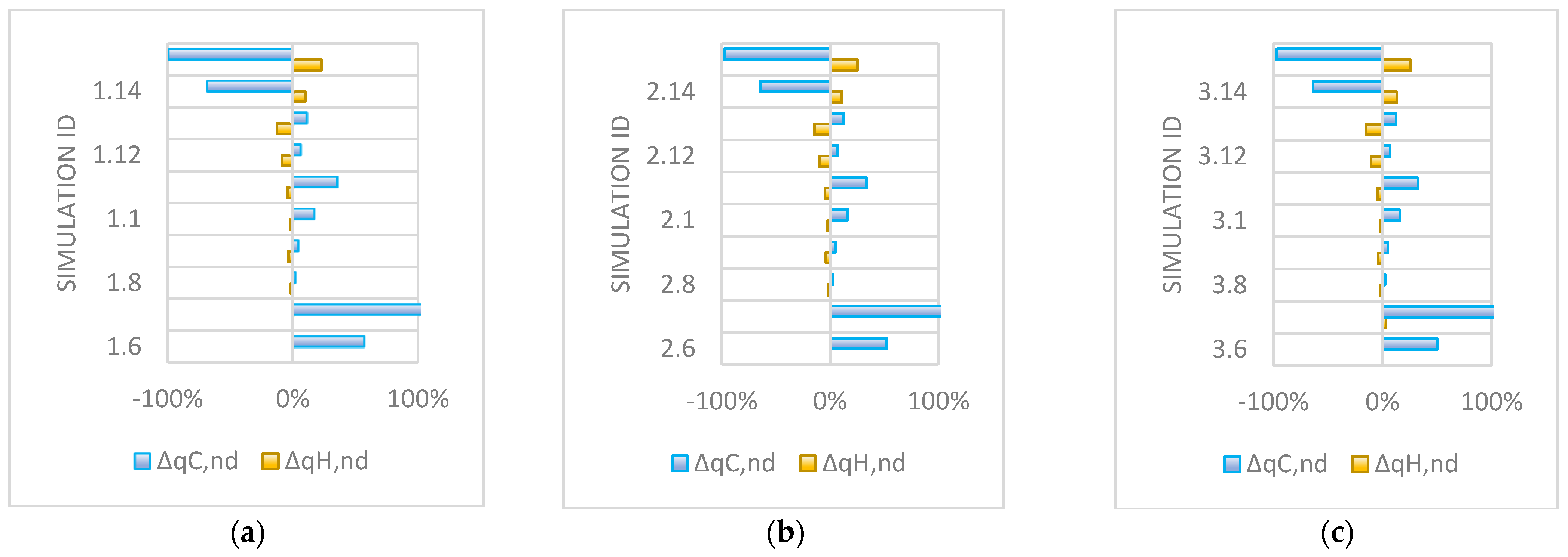
3.2. Simulation Results for Variations of Windows Parameters

The second set of simulations is related to the variation of input parameters describing the thermophysical properties and geometry of windows, as presented in

Table 12. Building I simulation results for varying parameters describing windows.

Building I (10 × 10)
Simulation ID	Description	qH,nd [kWh/m2]	Δ qH,nd	qC,nd [kWh/m2]	Δ qC,nd
1.6	Window to floor 25%	52.20	−0.54%	10.19	57.20%
1.7	Window to floor 30%	52.18	−0.57%	14.30	120.51%
1.8	Frame U-value 1.2 W/m2K	51.60	−1.69%	6.63	2.22%
1.9	Frame U-value 0.9 W/m2K	50.69	−3.43%	6.78	4.55%
1.10	FF = 0.25	51.33	−2.20%	7.60	17.22%
1.11	FF = 0.2	50.21	−4.33%	8.79	35.57%
1.12	Glazing U-value 0.88 W/m2K	47.91	−8.72%	6.90	6.44%
1.13	Glazing U-value 0.62 W/m2K	45.86	−12.63%	7.22	11.30%
1.14	Glazing g-value 0.42	57.74	10.00%	2.04	−68.49%
1.15	Glazing g-value 0.22	64.51	22.91%	0.04	−99.37%

,

Table 13. Building II simulation results for varying parameters describing windows.

Building II (20 × 20)
Simulation ID	Description	qH,nd [kWh/m2]	Δ qH,nd	qC,nd [kWh/m2]	Δ qC,nd
2.6	Window to floor 25%	45.49	−0.04%	11.37	52.19%
2.7	Window to floor 30%	45.74	0.51%	15.53	107.96%
2.8	Frame U-value 1.2 W/m2K	44.62	−1.94%	7.64	2.34%
2.9	Frame U-value 0.9 W/m2K	43.72	−3.93%	7.83	4.80%
2.10	Frame ratio 25%	44.43	−2.37%	8.68	16.29%
2.11	Frame ratio 20%	43.39	−4.65%	9.96	33.42%
2.12	Glazing U-value 0.88 W/m2K	40.93	−10.05%	7.98	6.81%
2.13	Glazing U-value 0.62 W/m2K	38.89	−14.53%	8.38	12.17%
2.14	Glazing g-value 0.42	50.47	10.91%	2.64	−64.64%
2.15	Glazing g-value 0.22	56.94	25.13%	0.16	−97.84%

and

Table 14. Building III simulation results for varying parameters describing windows.

Building III (30 × 30)
Simulation ID	Description	qH,nd [kWh/m2]	Δ qH,nd	qC,nd [kWh/m2]	Δ qC,nd
3.6	Window to floor 25%	43.37	0.23%	13.71	50.16%
3.7	Window to floor 30%	43.75	3.09%	15.85	103.18%
3.8	Frame U-value 1.2 W/m2K	42.39	−2.05%	7.99	2.38%
3.9	Frame U-value 0.9 W/m2K	43.48	−4.14%	8.18	4.88%
3.10	Frame ratio 25%	42.23	−2.42%	9.04	15.86%
3.11	Frame ratio 20%	43.22	−4.75%	10.34	32.50%
3.12	Glazing U-value 0.88 W/m2K	38.69	−10.60%	8.34	6.92%
3.13	Glazing U-value 0.62 W/m2K	36.64	−15.32%	8.78	12.50%
3.14	Glazing g-value 0.42	48.13	13.22%	2.83	−63.72%
3.15	Glazing g-value 0.22	54.47	25.88%	0.24	−96.98%

.

The results show that the most significant parameter is the solar heat gain coefficient (SHGC or g-value), for energy needed for both heating and cooling. With g-value reduced from the baseline value of 0.62 to 0.22, the energy needed for heating is increased from 22% for Building I (Table 12, simulation ID 1.15—glazing g-value = 0.22) to 25% for Buildings II and III (Table 13, simulation ID 2.15 and Table 14, simulation ID 3.15—glazing g-value = 0.22). The influence on simulated energy needed for cooling is even more significant, with Δ q_C,nd greater than 90% for all three buildings (simulation ID 1.15, 2.15, and 3.15).

Incremental changes of 5% for window to floor ratio (simulations ID x.6, x.7) result in a less than 1% incremental change in calculated annual energy for heating, but have an extreme impact on calculated annual energy needed for cooling, which increases by about 50% for every 5% increase in window to floor ratio, as illustrated in Figure 4.

The frame U-value is the least influential factor, and an 18% improvement in frame U-value results in only about 3% reduced energy needed for heating and about 5% change in calculated energy for cooling (simulations ID x.8, x.9). This is since the baseline windows frame factor is 30%, which means that window frame accounts for only 3.21%, 4.47%, and 5.63% of total envelope area for Buildings I, II, and III, respectively.

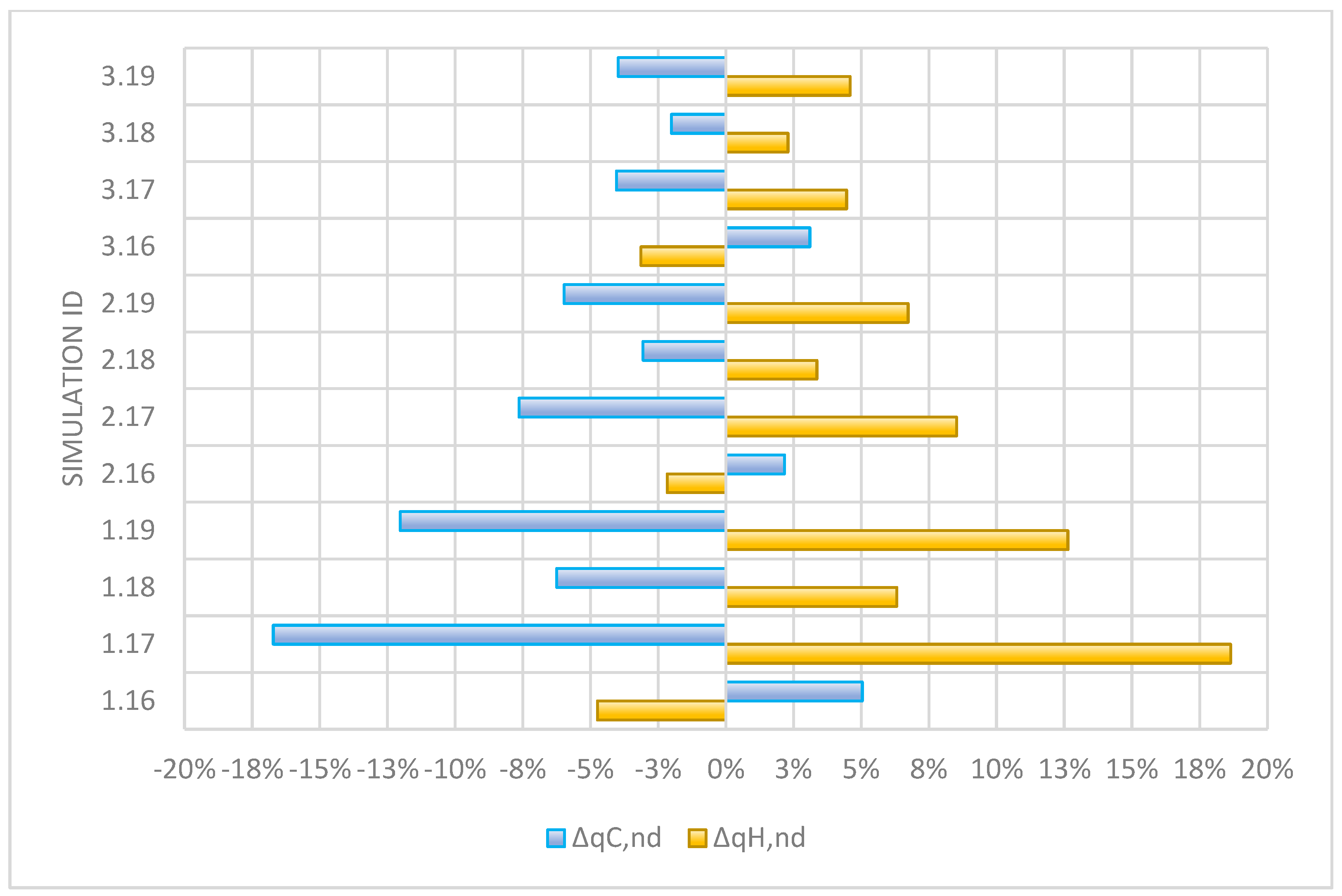
3.3. Simulation Results for Variations in External Wall Parameters

Variations in external wall parameters include U-value (simulations ID x.16, x.17) and thermal bridging (simulations ID x.18, x.19). Simulation results show significant and meaningful correlations between those modeling inputs and results, especially for Building I, with the highest BSF (

Table 15. Building I simulation results for varying external wall parameters.

Building I (10 × 10)
Simulation ID	Description	qH,nd [kWh/m2]	Δ qH,nd	qC,nd [kWh/m2]	Δ qC,nd
1.16	Ext. wall U-value 0.140 W/m2K	49.99	−4.75%	6.81	5.04%
1.17	Ext. wall U-value 0.315 W/m2K	62.27	18.64%	5.40	−16.72%
1.18	Thermal brid. ψ = 0.05 W/mK	55.79	6.31%	6.08	−6.25%
1.19	Thermal brid. ψ = 0.10 W/mK	59.11	12.63%	5.70	−12.03%

,

Table 16. Building II simulation results for varying external wall parameters.

Building II (20 × 20)
Simulation ID	Description	qH,nd [kWh/m2]	Δ qH,nd	qC,nd [kWh/m2]	Δ qC,nd
2.16	Ext. wall U-value 0.140 W/m2K	44.52	−2.17%	7.63	2.16%
2.17	Ext. wall U-value 0.315 W/m2K	49.38	8.52%	6.90	−7.65%
2.18	Thermal brid. ψ = 0.05 W/mK	47.04	3.36%	7.24	−3.06%
2.19	Thermal brid. ψ = 0.10 W/mK	48.57	6.73%	7.02	−5.98%

and

Table 17. Building III simulation results for varying external wall parameters.

Building III (30 × 30)
Simulation ID	Description	qH,nd [kWh/m2]	Δ qH,nd	qC,nd [kWh/m2]	Δ qC,nd
3.16	Ext. wall U-value 0.140 W/m2K	42.78	−3.14%	7.89	3.10%
3.17	Ext. wall U-value 0.315 W/m2K	45.21	4.46%	7.48	−4.05%
3.18	Thermal brid. ψ = 0.05 W/mK	44.27	2.29%	7.64	−2.02%
3.19	Thermal brid. ψ = 0.10 W/mK	45.26	4.59%	7.49	−3.98%

and Figure 5). The reduced influence of envelope input parameters with a decrease in BSF is also significant and illustrated in Figure 6, where absolute values for Δq_H,nd and Δq_C,nd are 18% and 17%, respectively, for Building I (simulation ID 1.17—ext. wall U-value = 0.315 W/m²K) with a BSF of 0.62 and dropping to below 5% for Building III with a BSF of 0.36 (simulation ID 3.17—ext. wall U-value = 0.315 W/m²K). This is because, with a reduction in BSF, the total share of heat conduction and radiation through the envelope is reduced on account of the increased share of convective heat transfer (infiltration). The same would apply if other energy flows are considered, such as internal heat gains from lighting, people, etc.

The inclusion of thermal bridging in the building energy model results in Δq_H,nd and Δq_C,nd of up to 12.63% and −12.03% in the case of I = 0.10 W/mK for Building I (simulation ID 1.19—thermal brid. Ψ = 0.10 W/mK), but also decreases to 4.59% and −3.98%, respectively, as BSF decreases (Building III, simulation ID 3.19—thermal brid. Ψ = 0.10 W/mK).

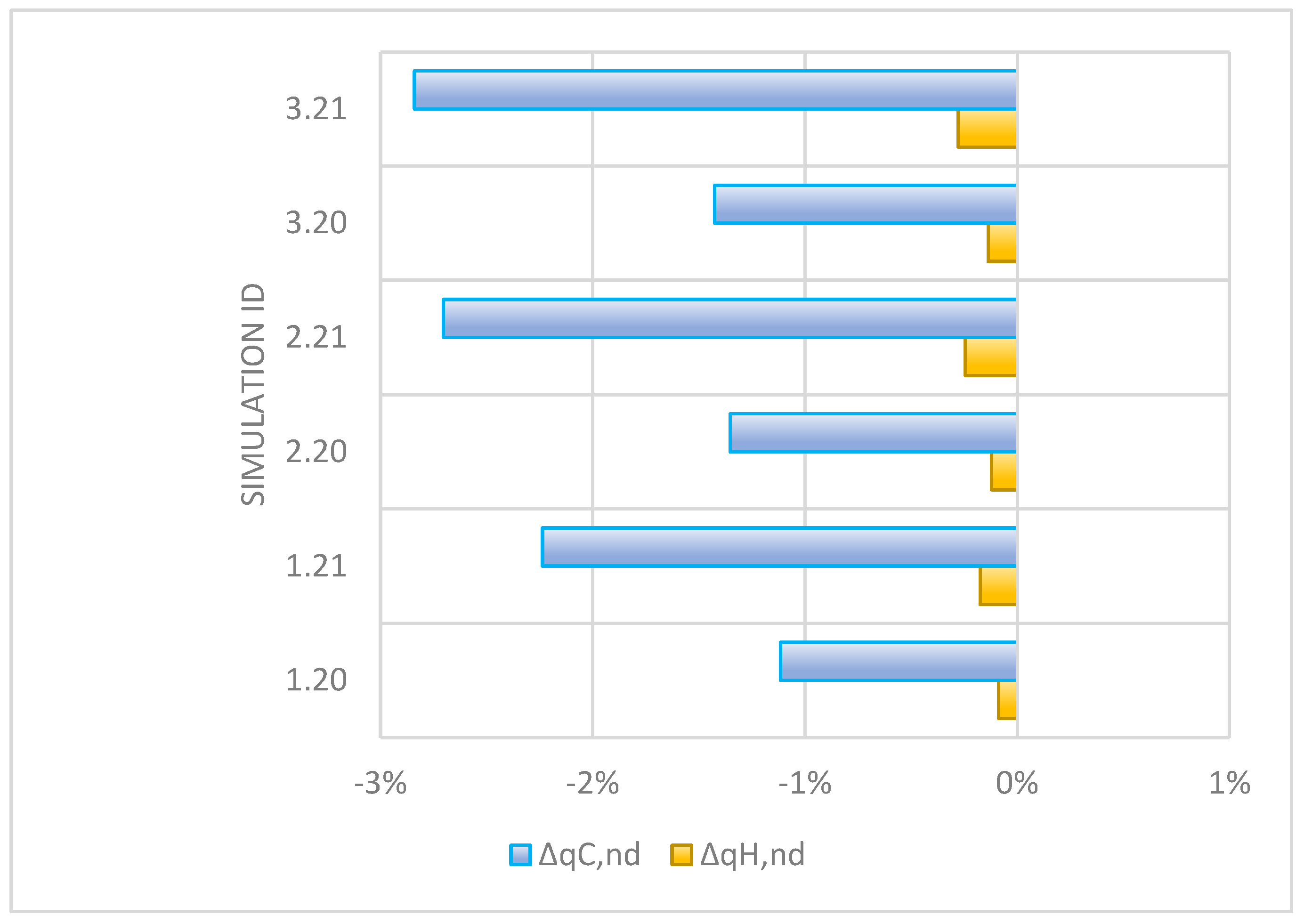
3.4. Simulation Results for Variation of Internal Volume Thermal Capacitance

Modeling the heat capacity of interior spaces is usually neglected in modeling practice, but the results presented in

Table 18. Building I simulation results for varying thermal capacitance of thermal zones.

Building I (10 × 10)
Simulation ID	Description	qH,nd [kWh/m2]	Δ qH,nd	qC,nd [kWh/m2]	Δ qC,nd
1.20	Heat capacity, 1% vol. furniture	52.44	−0.09%	6.41	−1.11%
1.21	Heat capacity, 2% vol. furniture	52.39	−0.17%	6.34	−2.24%

,

Table 19. Building II simulation results for varying thermal capacitance of thermal zones.

Building II (20 × 20)
Simulation ID	Description	qH,nd [kWh/m2]	Δ qH,nd	qC,nd [kWh/m2]	Δ qC,nd
3.16	Heat capacity, 1% vol. furniture	45.45	−0.12%	7.37	−1.35%
3.17	Heat capacity, 2% vol. furniture	45.39	−0.24%	7.27	−2.70%

and

Table 20. Building III simulation results for varying thermal capacitance of thermal zones.

Building III (30 × 30)
Simulation ID	Description	qH,nd [kWh/m2]	Δ qH,nd	qC,nd [kWh/m2]	Δ qC,nd
3.16	Heat capacity, 1% vol. furniture	43.22	−0.14%	7.69	−1.43%
3.17	Heat capacity, 2% vol. furniture	43.16	−0.28%	7.58	−2.84%

show that it should be considered, especially when estimating the annual energy needed for cooling. This is also illustrated in Figure 6, which shows that, for a 1% incremental increase in furniture volume to total internal volume ratio, the energy needed for cooling decreases by about 1%. The reason for this is that, during the peak cooling demand, when the mechanical cooling system is running, some solar gains are stored in the furniture thermal mass and later gradually removed during the period when the cooling peak demand has passed, when indoor air temperature is already below the cooling setpoint and the mechanical cooling is off.

4. Conclusions

This study has quantified, via dynamic TRNSYS simulations, how key envelope and model-geometry parameters affect annual heating (q_H,nd) and cooling (q_C,nd) demands per unit floor area for three theoretical buildings in Ljubljana, Slovenia.

For the configurations investigated, the glazing solar heat-gain coefficient (g-value) exerts the largest relative impact, lowering g from 0.62 to 0.22, increasing q_H,nd by 20–25%, and reducing q_C,nd by approximately 95%. However, this ranking of sensitivity applies only to the studied façades, window to floor ratios, and climate. In other climates or building designs, changes in glazing U-value or wall insulation may dominate.

Variations in infiltration modeling (ACH vs. volumetric flow) and the choice of modeled floor-area reference (internal, middle, external dimensions) produced up to ±20% swings in both q_H,nd and q_C,nd for the smallest, highest-shape-factor building (BSF = 0.62), but diminished to <6% for the largest (BSF = 0.36). This underscores the importance of consistent geometry and infiltration inputs, especially in compact, high-BSF designs.

Changes in frame U-value (±0.3 W/m²K) and external wall U-value (±0.14 W/m²K) yielded ≤15% variations in q_H,nd and <18% in q_C,nd, with greatest effects in the high-BSF case. Thermal bridging (ψ up to 0.10 W/mK) altered demands by up to ±12%. Interior thermal capacitance (1–2% furniture by volume) had a minor influence on heating but reduced cooling needs by 2–3%.

These findings, while derived from a specific case study involving theoretical buildings in the Ljubljana climate, offer insights that are largely generalizable. However, care must be taken when applying them to other contexts. Factors such as local climate, building orientation, and occupancy patterns can significantly influence the relative importance of individual parameters. Therefore, the sensitivity rankings established here should be interpreted with consideration for additional, case-specific conditions.

By providing a structured sensitivity map of envelope modeling inputs, this work supports building energy modelers, researchers [35], and practitioners in making more informed choices during model preparation. It highlights which inputs warrant greater accuracy and attention to avoid misrepresentation in simulation results. While broader applicability requires further studies across diverse building types and climates, the presented framework lays a foundation for prioritizing input accuracy in dynamic simulation environments.

References

1. Eurostat. Energy Statistics—Final Energy Consumption in the Residential Sector. Available online: https://ec.europa.eu/eurostat (accessed on 15 May 2025).
2. European Environment Agency (EEA). Final Energy Consumption by Sector and Fuel Type. Available online: https://www.eea.europa.eu (accessed on 15 May 2025).
3. Li, Y.; O’Neill, Z.; Zhang, L.; Chen, J.; Im, P.; DeGraw, J. Grey-box modeling and application for building energy simulations—A critical review. Renew. Sustain. Energy Rev. 2021, 146, 111174. [Google Scholar] [CrossRef]
4. Crawley, D.B.; Hand, J.W.; Kummert, M.; Griffith, B.T. Contrasting the capabilities of building energy performance simulation programs. Build. Environ. 2008, 43, 661–673. [Google Scholar] [CrossRef]
5. Ferrero, A.; Lenta, E.; Monetti, V.; Fabrizio, E.; Filippi, M.; To, G. How to apply building energy performance simulation at the various design stages: A recipes approach. In Proceedings of the 14th IBPSA Conference, Hyderabad, India, 7–9 December 2015; pp. 2286–2293. [Google Scholar]
6. Pacheco, R.; Ordóñez, J.; Martínez, G. Energy efficient design of buildings: A review. Renew. Sustain. Energy Rev. 2012, 16, 3559–3573. [Google Scholar] [CrossRef]
7. Zakula, T.; Bagaric, M.; Ferdelji, N.; Milovanovic, B.; Mudrinic, S.; Ritosa, K. Comparison of dynamic simulations and the ISO 52016 standard for the assessment of building energy performance. Appl. Energy 2019, 254, 113553. [Google Scholar] [CrossRef]
8. De Wilde, P. The gap between predicted and measured energy performance of buildings: A framework for investigation. Autom. Constr. 2014, 41, 40–49. [Google Scholar] [CrossRef]
9. Menezes, A.C.; Cripps, A.; Bouchlaghem, D.; Buswell, R. Predicted vs. actual energy performance of non-domestic buildings: Using post-occupancy evaluation data to reduce the performance gap. Appl. Energy 2012, 97, 355–364. [Google Scholar] [CrossRef]
10. De Wit, S.; Augenbroe, G. Analysis of uncertainty in building design evaluations and its implications. Energy Build. 2002, 34, 951–958. [Google Scholar] [CrossRef]
11. Rugani, R.; Picco, M.; Salvadori, G.; Fantozzi, F.; Marengo, M. A numerical analysis of occupancy profile databases impact on dynamic energy simulation of buildings. Energy Build. 2024, 310, 114114. [Google Scholar] [CrossRef]
12. Oldewurtel, F.; Sturzenegger, D.; Morari, M. Importance of occupancy information for building climate control. Appl. Energy 2013, 101, 521–532. [Google Scholar] [CrossRef]
13. Viganò, G.S.M.; Rugani, R.; Marengo, M.; Picco, M. Assessing the impact of climate change on building energy performance: A future-oriented analysis on the UK. Architecture 2024, 4, 1201–1224. [Google Scholar] [CrossRef]
14. Saltelli, A.; Chan, K.; Scott, E.M. Sensitivity Analysis: Gauging the Worth of Scientific Models; Wiley: New York, NY, USA, 2000. [Google Scholar]
15. Capozzoli, A.; Mechri, H.E.; Corrado, V. Impacts of Architectural Design Choices on Building Energy Performance—Applications of Uncertainty and Sensitivity Techniques. In Proceedings of the 11th International IBPSA Conference, Glasgow, UK, 27–30 July 2009. [Google Scholar]
16. Hensen, J.L.M.; Lamberts, R. Building Performance Simulation for Design and Operation, 2nd ed.; Routledge: London, UK, 2019. [Google Scholar]
17. Wang, S.; Yan, C.; Xiao, F. Quantitative energy performance assessment methods for existing buildings. Energy Build. 2012, 55, 873–888. [Google Scholar] [CrossRef]
18. Dermentzis, G.; Ochs, F.; Gustafsson, M.; Calabrese, T.; Siegele, D.; Feist, W.; Dipasquale, C.; Fedrizzi, R.; Bales, C. A comprehensive evaluation of a monthly-based energy auditing tool through dynamic simulations, and monitoring in a renovation case study. Energy Build. 2019, 183, 713–726. [Google Scholar] [CrossRef]
19. Nageler, P.; Schweiger, G.; Pichler, M.; Brandl, D.; Mach, T.; Heimrath, R.; Schranzhofer, H.; Hochenauer, C. Validation of dynamic building energy simulation tools based on a real test-box with thermally activated building systems (TABS). Energy Build. 2018, 168, 42–55. [Google Scholar] [CrossRef]
20. Mangi, M.; Ochs, F.; de Vries, S.; Maccarini, A.; Sigg, F. Detailed cross comparison of building energy simulation tools results using a reference office building as a case study. Energy Build. 2021, 250, 111260. [Google Scholar] [CrossRef]
21. Calleja Rodríguez, G.; Carrillo Andrés, A.; Domínguez Muñoz, F.; Cejudo López, J.M.; Zhang, Y. Uncertainties and sensitivity analysis in building energy simulation using macroparameters. Energy Build. 2013, 67, 79–87. [Google Scholar] [CrossRef]
22. Connolly, D.; Lund, H.; Mathiesen, B.V.; Leahy, M. A review of computer tools for analysing the integration of renewable energy into various energy systems. Appl. Energy 2010, 87, 1059–1082. [Google Scholar] [CrossRef]
23. Gelesz, A.; Catto Lucchino, E.; Goia, F.; Serra, V.; Reith, A. Characteristics that matter in a climate façade: A sensitivity analysis with building energy simulation tools. Energy Build. 2020, 229, 110467. [Google Scholar] [CrossRef]
24. Mazzeo, D.; Matera, N.; Cornaro, C.; Oliveti, G.; Romagnoni, P.; De Santoli, L. EnergyPlus, IDA ICE and TRNSYS predictive simulation accuracy for building thermal behaviour evaluation by using an experimental campaign in solar test boxes with and without a PCM module. Energy Build. 2020, 212, 109812. [Google Scholar] [CrossRef]
25. Klein, S.A.; Beckman, W.A.; Mitchell, J.W.; Duffie, J.A.; Duffie, N.A.; Freeman, T.L.; Mitchell, J.C.; Braun, J.E.; Evans, B.L.; Kummer, J.P.; et al. TRNSYS 18: A Transient System Simulation Program; University of Wisconsin: Madison, WI, USA, 2017. [Google Scholar]
26. Republic of Slovenia, Ministry of the Environment and Spatial Planning. Pures 2010: Rules on Efficient Use of Energy in Buildings; Off. Gaz. Repub. Slov. No. 52/2010, 30 June 2010; Republic of Slovenia, Ministry of the Environment and Spatial Planning: Ljubljana, Slovenia, 2010; pp. 8315–8354.
27. ISO 7730; Ergonomics of the Thermal Environment—Analytical Determination and Interpretation of Thermal Comfort Using Calculation of the PMV and PPD Indices and Local Thermal Comfort Criteria. International Organization for Standardization: Geneva, Switzerland, 2005.
28. Šijanec Zavrl, M.; Zbašnik-Senegačnik, M.; Kristl, Ž. Building Typologies and Energy Renovation Scenarios in Slovenia. Energy Policy 2020, 140, 111424. [Google Scholar] [CrossRef]
29. Dolinar, M.; Vidrih, B.; Zavrl, M. Assessment of the energy performance of the existing residential building stock in Slovenia. Energy Build. 2017, 152, 163–175. [Google Scholar] [CrossRef]
30. Canadian Commission on Building and Fire Codes; National Research Council of Canada. National Energy Code of Canada for Buildings 2017; National Research Council of Canada: Ottawa, ON, Canada, 2017.
31. Scott West, P.E.; Ndiaye, D. Energy simulation aided design for buildings. ASHRAE J. 2019, 61, 20–26. [Google Scholar]
32. Ge, H.; Baba, F. Dynamic effect of thermal bridges on the energy performance of a low-rise residential building. Energy Build. 2015, 105, 106–118. [Google Scholar] [CrossRef]
33. Al-Sanea, S.A.; Zedan, M.F. Effect of thermal bridges on transmission loads and thermal resistance of building walls under dynamic conditions. Appl. Energy 2012, 98, 584–593. [Google Scholar] [CrossRef]
34. Johra, H.; Heiselberg, P. Influence of internal thermal mass on the indoor thermal dynamics and integration of phase change materials in furniture for building energy storage: A review. Renew. Sustain. Energy Rev. 2017, 69, 19–32. [Google Scholar] [CrossRef]
35. Zhang, Y.; Omer, S.; Hu, R. Impact of window size modification on energy consumption in UK residential buildings: A feasibility and simulation study. Sustainability 2025, 17, 3258. [Google Scholar] [CrossRef]
Figure 1. Three baseline building sizes/geometries: (a) 10 × 10 × 9 m; (b) 20 × 20 × 9 m; (c) 30 × 30 × 9 m.
Sustainability 17 05276 g001
Figure 2. Modeled floor area per (a) internal, (b) middle, or (c) external dimensions.
Sustainability 17 05276 g002
Figure 3. Correlation between referent MFA dimensions and relative change in simulated energy performance.
Sustainability 17 05276 g003
Figure 4. Correlation between model windows parameters and relative change in simulated energy performance for (a) Building I; (b) Building II; (c) Building III.
Sustainability 17 05276 g004
Figure 5. Correlation between model thermal capacitance of thermal zones and relative change in simulated energy performance.
Sustainability 17 05276 g005
Figure 6. Correlation between model external wall parameters and relative change in simulated energy performance.
Sustainability 17 05276 g006