Article

Comparison of Selected Ensemble Supervised Learning Algorithms Used for Meteorological Normalisation of Particulate Matter (PM10)

Faculty of Geo-Data Science, Geodesy and Environmental Engineering, AGH University of Krakow, 30-059 Kraków, Poland
*
Author to whom correspondence should be addressed.
Sustainability 2025, 17(12), 5274; https://doi.org/10.3390/su17125274
Submission received: 23 April 2025 / Revised: 25 May 2025 / Accepted: 4 June 2025 / Published: 7 June 2025
(This article belongs to the Section Pollution Prevention, Mitigation and Sustainability)

Abstract

Air pollution, particularly PM10 particulate matter, poses significant health risks related to respiratory and cardiovascular diseases as well as cancer. Accurate identification of PM10 reduction factors is therefore essential for developing effective sustainable development strategies. According to the current state of knowledge, machine learning methods are most frequently employed for this purpose due to their superior performance compared to classical statistical approaches. This study evaluated the performance of three machine learning algorithms—Decision Tree (CART), Random Forest, and Cubist Rule—in predicting PM10 concentrations and estimating long-term trends following meteorological normalisation. The research focused on Tarnów, Poland (2010–2022), with comprehensive consideration of meteorological variability. The results demonstrated superior accuracy for the Random Forest and Cubist models (R2 ~0.88–0.89, RMSE ~14 μg/m3) compared to CART (RMSE 19.96 μg/m3). Air temperature and boundary layer height emerged as the most significant predictive variables across all algorithms. The Cubist algorithm proved particularly effective in detecting the impact of policy interventions, making it valuable for air quality trend analysis. While the study confirmed a statistically significant annual decrease in PM10 concentrations (0.83–1.03 μg/m3), pollution levels still exceeded both the updated EU air quality standards from 2024 (Directive (EU) 2024/2881), which will come into force in 2030, and the more stringent WHO guidelines from 2021.

1. Introduction

PM10 contamination in the air has a strong impact on human health. According to the International Agency for Research on Cancer (IARC), air pollution is considered a mixture of potentially carcinogenic substances. PM10 particles can penetrate deep into the lungs, contributing to respiratory and cardiovascular problems. This impact is comparable to other significant health risks, such as tobacco smoking or an unhealthy diet. Long-term exposure is associated with reduced lung function, worsened asthma symptoms, and respiratory infections, especially in children. Among adults, the risk of ischemic heart disease and stroke increases—both of which are major causes of premature death linked to air pollution [1,2,3,4,5,6]. In Poland, the number of premature deaths caused by particulate pollution was approximately 44,000 in 2012 and 43,000 in 2019 [1,6,7]. Recent studies indicate that in Poland, this number may be as high as 67,000 premature deaths [8].
An effective assessment of air pollution concentration trends is possible through the application of meteorological normalisation. This method was developed by Stuart K. Grange and David C. Carslaw [9,10] and makes it possible to eliminate the influence of meteorological conditions from the time series of air pollution concentrations. Meteorological normalisation (also known as deweathering) involves generating multiple concentration forecasts for random meteorological scenarios using developed supervised learning models, with the resulting values being averaged. As a result, it becomes possible to estimate non-parametric trend values of air pollution concentrations corresponding to averaged meteorological conditions. Meteorological normalisation is a relatively new method that has been used by many researchers for various scientific purposes in different regions of the world. Previous studies have been conducted, among others, in the United Kingdom, Switzerland, Italy, Spain, Croatia, Poland, Australia, China, and Iran, demonstrating the universality of the normalisation method regardless of geographic location [9,10,11,12,13,14,15,16,17,18,19,20,21,22,23,24,25].
The Random Forest (RF) algorithm is commonly used in meteorological normalisation due to its robustness to missing data, multicollinearity among explanatory variables, and the relative simplicity of hyperparameter tuning [10,11,16]. Besides RF, the Gradient Boosted Regression Model (GBM) algorithm has also often been used for meteorological normalisation [12,14]. These two algorithms are most often compared to each other because both are characterised by a high prediction accuracy and low bias [1,5,9,16]. Mallet (2021) [24] conducted an experiment to compare the aforementioned methods. The GBM was able to explain 46% of the predicted variable (PM10). In the case of the Random Forest model, the coefficient of determination (R2) was 0.59, indicating that this model explained 59% of the variance in the predicted variable. Comparing the RF and GBM algorithms in terms of NOx prediction, the values of the coefficient of determination were 0.73 and 0.76, respectively [17]. Moreover, it was shown that the Random Forest algorithm is characterised by lower systematic errors. Lovrić et al. (2022) [13] compared the Random Forest algorithm (RF) and the Gradient Boosting Method (LightGBM) for predicting concentrations of particulate matters. In this case, they obtained similar results from the above models. RF achieved an R2 value of 0.78 and LightGBM achieved a value of 0.77. The study conducted in London showed that the Random Forest algorithm has varying accuracy depending on the predicted substance (SO2, NO2, and NOx). For NOx and NO2 on Marylebone Road, R2 values of 0.82 and 0.83 were achieved, respectively. However, for SO2, the R2 results were significantly lower, ranging from 0.63 to 0.67 [9]. This means that the methods under consideration have varying accuracy depending on the location of the study and the predicted substance. This is also confirmed by the studies carried out for three Chinese mega cities, where for many substances (PM2.5, PM10, NO2, SO2, CO, and O3), R2 values ranging from 0.7 to 0.86 were obtained using the Random Forest algorithm [16].
The aim of this study was to compare the effectiveness of three machine learning models (Decision Tree, Random Forest, and Cubist Rules) in forecasting and estimating trends in PM10 concentrations based on normalised data. This task was undertaken due to the lack of comprehensive comparative analyses of various supervised learning algorithms regarding their impact on nonparametric estimation of pollution trends. In the study, boosted methods (GBM, LightGBM) were intentionally omitted, as the literature [9,13,24] indicates that they demonstrate comparable or lower accuracy compared to the Random Forest algorithm. Only Gagliardi and Andenna (2021) [17] observed slightly higher R2 (0.76 vs. 0.73) for GBM; however, other metrics did not confirm its superiority. It was decided to use the Cubist Rules algorithm [26,27], which—unlike other ensemble methods—has not been used in meteorological normalisation yet. Its advantage is the better interpretability of its results and its ability to generate transparent decision rules while maintaining high accuracy. It is an ensemble algorithm that combines a tree-based approach with rule generation.
The Cubist Rules algorithm has been widely used in numerous air quality studies. It has been applied for forecasting the spatiotemporal distributions of PM2.5 concentrations [28,29], identifying determinants of ozone concentrations [30], and investigating correlations between air pollution and social poverty [31], among other applications. According to the literature review conducted by Méndez et al. (2023) [32], this study focused exclusively on machine learning methods. Compared to classical statistical approaches such as linear regression, ARIMA models, and ridge regression, machine learning techniques are widely applied across various geographic regions due to their ability to model nonlinear relationships, handle multicollinearity among explanatory variables, manage missing data effectively, and achieve high predictive accuracy. Recent studies indicate that machine learning methods often outperform traditional statistical techniques—including ridge regression, which, despite its robustness to multicollinearity, tends to exhibit lower predictive performance when applied to complex air quality datasets [33]. On the other hand, it should be emphasised that more advanced methods, such as RNN (recurrent neural networks) and ANN (artificial neural networks), exhibit lower accuracy in forecasting PM10 concentrations in urban areas compared to ensemble tree-based methods [34].
This study provides a comprehensive analysis of various machine learning algorithms applied to meteorological normalisation and PM10 concentration trend assessment. Section 2 presents the research framework, beginning with the geographical and demographic characterisation of the study area (Tarnów, Poland) in Section 2.1, followed by a detailed description of data sources (air quality monitoring, meteorological measurements, and ERA5 reanalysis) and computational methods in Section 2.2. This includes the selection of predictor variables, model validation protocols, and implementation specifics for the three machine learning algorithms (CART, Random Forest, and Cubist Rules). Section 3 provides a systematic evaluation of results, where Section 3.1 compares algorithm performance through predictive accuracy metrics, Section 3.2 analyses variable importance patterns, and Section 3.3 interprets the derived PM10 concentration trends after meteorological normalisation. The discussion contextualises these findings against the existing literature while highlighting methodological implications. Finally, Section 4 synthesises the practical applications for air quality management and proposes targeted directions for improving predictive modelling in environmental policy contexts.

2. Materials and Methods
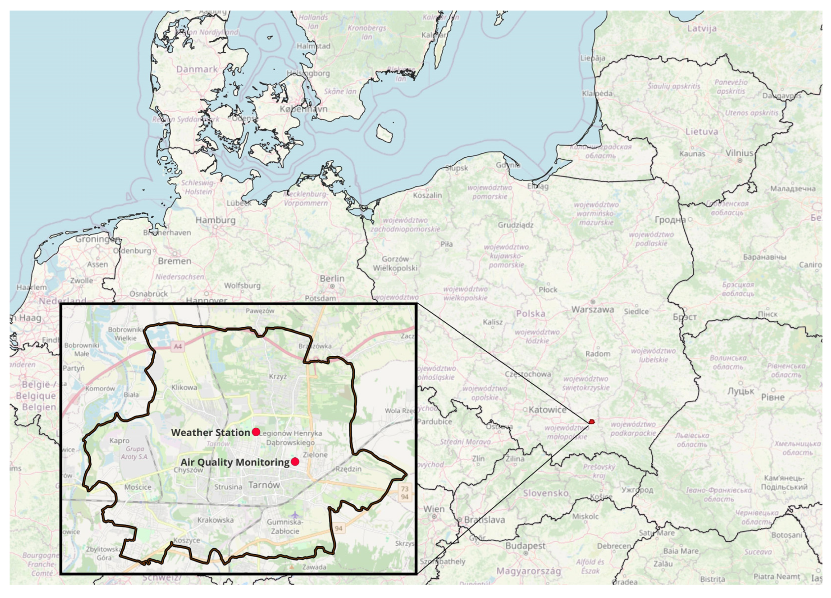
2.1. Research Area

The location of the research area, along with the air quality monitoring station and the meteorological station, is shown in Figure 1. The city of Tarnów is located in the eastern part of the Małopolska voivodeship in Poland. It is located on the Tarnów Plateau at the boundary between the Sandomierz Basin and the Carpathian Foothills. The city is inhabited by 103,130 people (data for the year 2023). The area of the city is 72.38 km2.
The analysed period covered the years 2010–2022. During this time, a significant improvement in air quality was observed in terms of PM10 concentrations. The current allowable average annual level of PM10 concentration is 40 μg/m3. This limit was exceeded in the first three analysed years. The year 2013 was omitted due to data completeness being less than 50%. A decrease in PM10 concentrations was observed from 41.9 μg/m3 (2010) to 23.7 μg/m3 (2022) (Figure 2). Despite the 43.4% reduction over the years, the average annual PM10 concentrations are still higher than the values set out in the recommendations issued by the WHO in 2021 (15 μg/m3) and the new guidelines adopted by the Council of the European Union in November 2024 (20 μg/m3). It was also found that the daily average standard was not met during the years 2010–2021 (Figure 3). Currently, it is permissible for air quality standards to be exceeded on 35 days per year, but the revised EU regulations [35] reduce this number to 18. Over the 12-year study period, two years (2010 and 2012) exceeded the annual limit and only four (2015, 2019, 2020 and 2022) had fewer than thirty-five days per year on which the daily limit was exceeded.

2.2. Data Sources and Computational Methods

The data for hourly PM10 concentration for the period 2010–2022 were obtained from the database of the Chief Inspectorate of Environmental Protection [36], while meteorological data such as wind speed (ws), wind direction (wd), relative humidity (rh), air temperature (tt), and atmospheric pressure (pres) were obtained from the archives of the Institute of Meteorology and Water Management [37]. Boundary layer height (blh), cloud base height (cbh), and surface net solar radiation (ssr) was obtained from reanalysis for the global climate and weather ERA5 [38]. The complete dataset used in this study is provided in the Supplementary Materials (Table S1).
The study compared three supervised learning algorithms classified as ensemble methods: Decision Tree (CART) [39], Random Forest (Ranger) [40,41], and Cubist Rules (Cubist) [26]. Decision Tree builds a single decision tree by recursively splitting the data based on predictor variables, which makes it simple and interpretable, though often prone to overfitting. Random Forest overcomes this limitation by creating an ensemble of trees using bootstrapped samples and random subsets of predictors, resulting in improved accuracy and robustness. Cubist Rules, on the other hand, combines Decision Tree with linear regression models in the terminal nodes, offering a hybrid approach that captures both nonlinear relationships and linear trends in the data [26,39,40,41]. Based on the date, auxiliary variables were created, such as day of the year according to the Julian calendar (jday), day of the week (wday), and hour of the day (hour), representing typical periods of changes in air pollution emissions due to anthropogenic activities. The date variable was converted into a numerical format of the date to reflect the trend. The dataset was divided into a training (80% of samples used to adjust the model parameters) set and test (20% of samples used to evaluate the model performance) set. From the training set, a validation set was created for the purpose of applying the resampling method (10-fold cross-validation). The use of this method provides a reasonable estimation of model accuracy assessment parameters at a level similar to the test set during the hyperparameter tuning stage of individual algorithms. For hyperparameter optimisation, a racing method was applied based on the statistical significance of the configurations of individual algorithms from the ANOVA model [42]. The application of this method allowed for a reduction in computation time by approximately 20%. The best-performing algorithms were evaluated on the test set. The evaluation of the model was carried out using basic statistical metrics, i.e., FAC2 (fraction of predictions within a factor of two), MB (mean bias), MGE (mean gross error), NMB (normalised mean bias), NMGE (normalised mean gross error), RMSE (root mean squared error), r (Pearson correlation coefficient), COE (coefficient of efficiency), and IOA (Index of Agreement based on Willmott) [43] (see Table A1 in Appendix A for more details).
In order to determine the importance of predicted variables, EMA (Exploratory Model Analysis) was conducted. The identification aimed to determine which meteorological data has the greatest impact on PM10 concentration. This method demonstrated how the model’s performance would change when one of the variables was removed. The significance was presented as RMSE values. The higher the metric, the greater the importance of the explanatory variable. The use of RMSE as a consistent metric enabled uniform comparisons of the applied supervised learning algorithms [44].
The developed models were used to carry out meteorological normalisation of particulate matter (PM10). For this purpose, we used bootstrap [45] with the number of repetitions equal to 200 for each data record. Based on normalised data determined using three models (CART, Ranger, Cubist), the PM10 trend was identified using the Theil–Sen robust linear regression estimator [46].

3. Result and Discussion

3.1. Evaluating the Accuracy of Machine Learning Algorithms

Figure 4 shows a comparison of observations with modelling results based on the applied algorithm. Three reference lines were added to the plot. One of them represents perfect mapping, while the other two indicate the error margin corresponding to a twofold overestimation or underestimation. All models accurately predict PM10 concentrations below 100 µg/m3, as evidenced by the high density of observations along the ideal model line. Nonetheless, regardless of the applied algorithm, there are instances of twofold overestimations and underestimations of PM10 concentrations. According to FAC2 values (shown in Table 1), the frequency did not exceed 10% when using the Random Forest (Ranger) and Cubist Rules (Cubist). In the case of the Decision Tree algorithm (CART), the frequency was almost twice as high. It is worth noting that the obtained FAC2 values for the Random Forest and Cubist Rules are comparable to those reported in other studies. Lv et al. (2022) [16], using the Random Forest model for PM10, achieved an FAC2 value of 0.91.
Table 1 summarises the statistical metrics used to assess the accuracy of models based on the machine learning algorithm. For the Ranger and Cubist algorithms, similar accuracy metric values were obtained. The values of the normalised mean gross error (NMGE), the coefficient of efficiency (COE), and the Index of Agreement (IOA) are the same. Ranger reached the highest value for the correlation coefficient (r), 0.89, while Cubist had a slightly lower score, 0.88. The models differed by RMSE by 0.03 μg/m3. The models had opposite values of mean bias (MB). For Ranger, the parameter assumed a positive value, which indicates a tendency to overestimate the results. The negative result obtained for CART and Cubist indicates a tendency to underestimate the results. For all three models, the normalised mean bias (NMB) value hovered around zero, indicating that no model had a significant tendency to overestimate or underestimate. The statistics for the CART algorithm significantly deviate from those of the other two models. RMSE reached its highest value of 19.96 μg/m3. NMGE indicated that the uncertainty of the Ranger algorithm’s forecasts occurs at a level of 39% of the mean value.
Compared to other studies, the machine learning models applied in this analysis exhibit varied effectiveness. Lv et al. (2022) [16] achieved a higher mean systematic error (MB ~0.11) with lower NMB and NMGE values, while the Random Forest model developed by Lovrić et al. (2022) [13] demonstrated a lower RMSE (10.47) compared to Mallet’s (2021) [24] result of 19.5. The best accuracy in terms of RMSE (5.39 µg/m3) was demonstrated by Gagliardi and Andenna (2021) [17], maintaining the same IOA value (0.76) and a slightly lower R2 (0.73). However, this model pertained to nitrogen oxide (NOx) concentrations. In terms of the coefficient of determination R2, the presented Random Forest (RF) model outperforms Mallet (2021) [24] (0.49–0.59), Grange and Carslaw (2019) [9] (0.54–0.71), and Gagliardi and Andenna (2021) [17], approaching the results achieved by Lv et al. [16] (0.81–0.94) and Wu et al. (2022) [25] (0.52–0.94). These findings confirm that the effectiveness of models depends both on the applied algorithm and the specificity of the analysed environmental data. Additionally, the appropriate selection of parameters and consideration of the local context are crucial for accurate air quality modelling.
The presented results of model accuracy evaluation are clearly superior compared to classical air pollution dispersion modelling techniques [47,48]. This is particularly important considering that traditional air quality models based on the Gaussian plume equation (e.g., ADMS, AERMOD, CALPUFF) can accurately predict only the distributions of the highest one-hour concentrations, most often expressed as the robust highest concentration (RHC). However, these models are unable to accurately reproduce the timing and location of peak concentrations [47,49,50,51]. On the other hand, classical approaches can be applied to any location since they do not require access to continuous air quality monitoring data. In contrast, machine-learning-based models are representative only for the location in which they were trained, making it impossible to directly apply them under different environmental conditions. Moreover, a separate ML model must be developed for each pollutant type, mainly due to the lack of information on the emission field or orographic constraints. Both groups of methods (classical and machine learning) have their limitations, but under appropriate conditions, they can complement each other. Their combined use may provide valuable insights, enabling a better understanding of the influence of various factors on air quality.

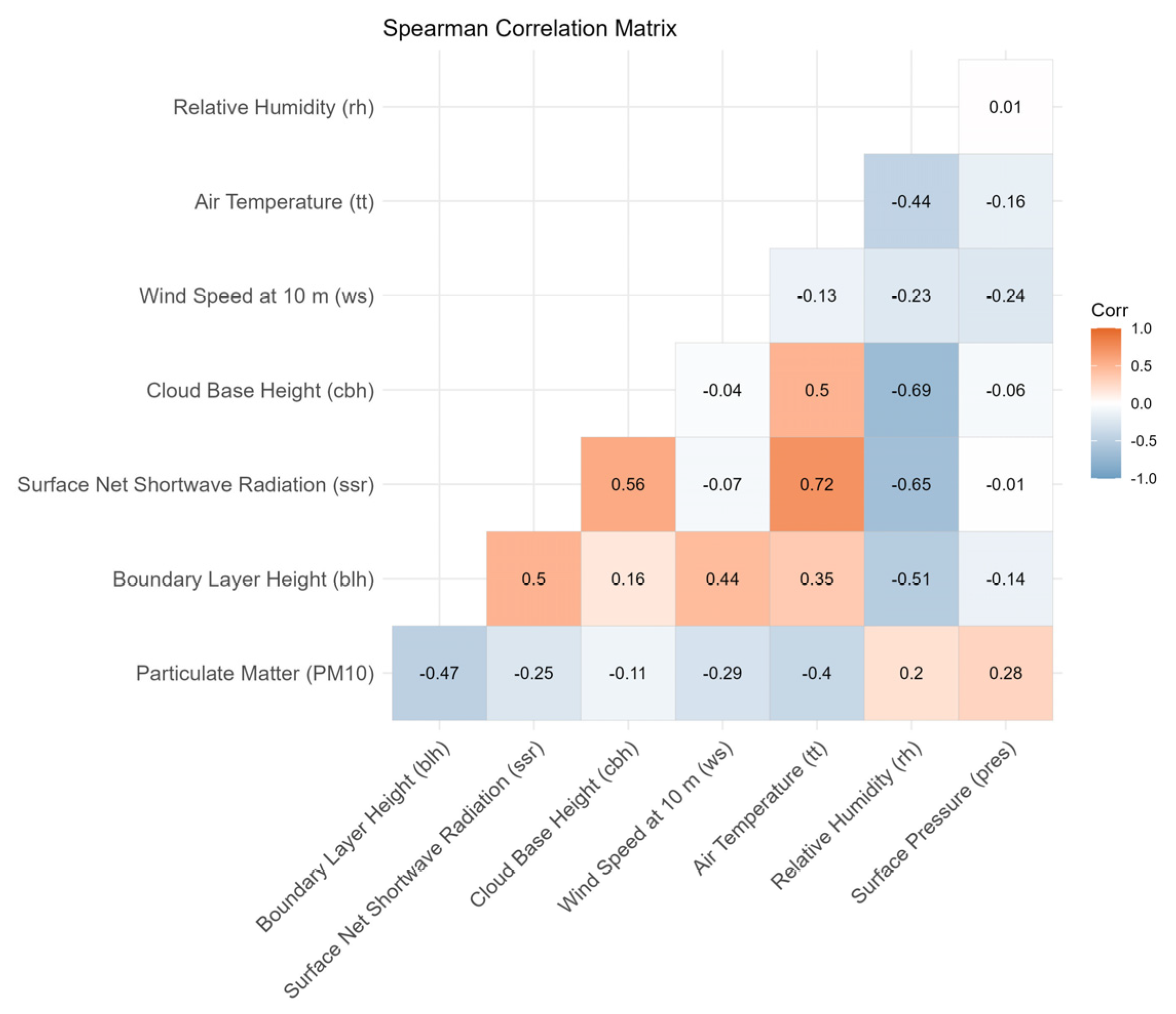
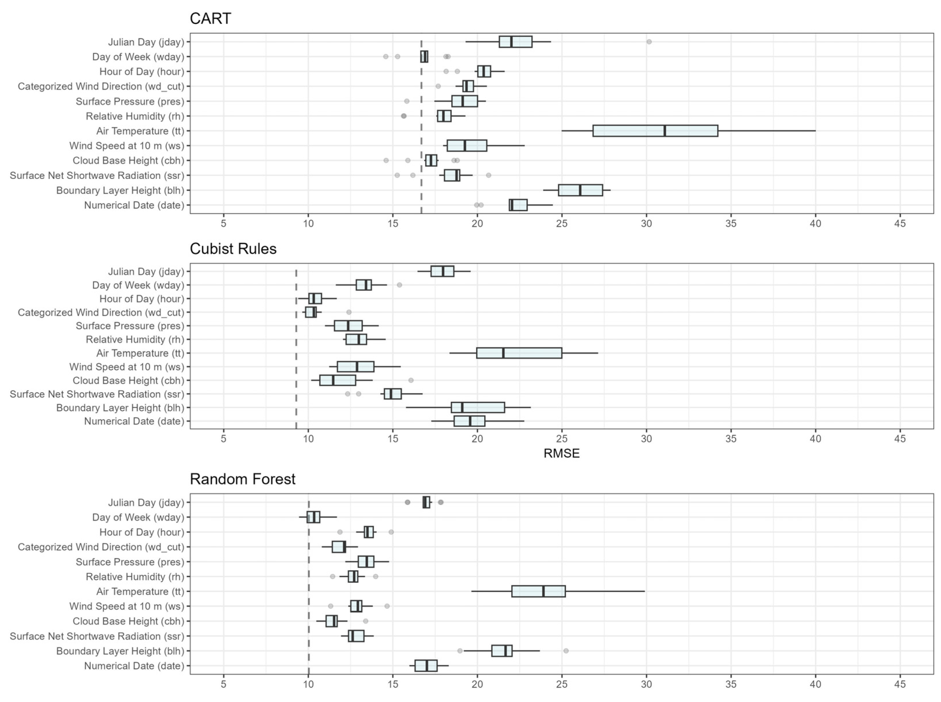
3.2. Importance Variable

The plot of the evaluation of the importance of an explanatory variable is shown in Figure 5. Boxplots demonstrate the change in the RMSE value after deleting individual variables [44,52]. The line inside the box indicates the median for the series of permutations, while the grey dots represent outlier values. The dashed vertical lines denote the loss function values for each model. The value of the loss function is constant and depends on model structure. It reflects error in the absence of predictive variables. For CART, the value is 16.69 μg/m3, for Ranger it is 10.03 μg/m3, and for Cubist it is 9.29 μg/m3. The values of the loss function were similar for Ranger and Cubist. In all the applied algorithms, air temperature (tt) turned out to be the variable with the greatest impact on PM10 concentrations. The median error after removing this variable was 23.9 μg/m3 (Ranger), 21.5 μg/m3 (Cubist), and 31.6 μg/m3 (CART). The significant impact of temperature likely stems from its association with the seasonal variability of emissions in the municipal and residential sector [53] and the deterioration of the conditions of dispersion of pollutants in winter, associated with the frequent occurrence of stable atmospheric layers [54]. It is worth noting that the Decision Tree algorithm (CART) showed a particularly strong dependence on the variable temperature compared to other models. This is a consequence of the collinearity of explanatory variables. In this case, the tuning process focused on a single variable (tt), which is highly correlated with the dependent variable (PM10) (Figure A1).
Other variables affecting the result were boundary layer height (blh), date (date), and the day of the year according to the Julian calendar (jday). In the case of the Ranger algorithm, removing the blh variable increased the median RMSE to 21.7 μg/m3, while for Cubist, the median increased to 19.1 μg/m3, and for CART, it increased to 26.1 μg/m3. Boundary layer height is associated with surface temperature inversion. This phenomenon at low elevation negatively affects the dispersion of pollutants. During weak air mass movements, PM10 concentrations accumulate at ground level [55,56]. The variable numerically defining the date is significant because it reflects changes in pollutant emissions. After removing the “date” variable, RMSE increased to 16.9 μg/m3 in Ranger, in Cubist, it increased to 18.0 μg/m3, and in CART, it increased to 22.0 μg/m3. For Decision Tree, the least significant variable turned out to be the one representing the day of the week (wday). Its removal resulted in an RMSE increase of only 0.2 μg/m3 compared to the value of the loss function for this model. The second variable that slightly impacts the prediction quality is cloud base height (cbh). The increase in RMSE for this parameter was only 0.6 μgm−3 compared to the value of the loss function. Calculations performed on the Cubist model indicated a low impact of the direction of wind (wd_cut) and the variable representing the hour of measurement during the day (hour). For both variables, RMSE increased by just 1 μg/m3 compared to the value of the loss function.
In each model, the temperature (tt) and the boundary layer height (blh) were the most important. The results obtained are not always consistent with earlier studies on other types of pollution and localisation. For example, studies conducted in the Alps focusing on nitrogen dioxide (NO2) revealed that the most important explanatory variable was temperature, while the second most significant variable was the day of the year according to the Julian calendar (jday) [18]. The high importance of jday resulted from the fact that studies conducted in the Alps did not consider the blh variable, focusing only on the temperature gradient.
On the other hand, studies conducted in Australia on PM10 revealed that the intensity of fires, trend, and temperature were more significant compared to wind speed and the boundary layer height. Other studies conducted in England on SO2, NO2, and NOx provided evidence of the high significance of wind speed (ws) compared to temperature [9]. This stands in opposition to the obtained research findings, though it relates specifically to gaseous air pollutants. However, as in the present study, variables such as the day of the year according to the Julian calendar (jday), hour (hour), and wind direction (wd_cut) were of little importance. Research conducted in southern Italy on NOx showed that the most significant variable was wind direction (wd_cut). This contrasts sharply with the findings of the presented studies, where this was typically a variable of little importance. It is essential to emphasise that the interpretation of the significance of explanatory variables depends on the type of substance and the location. The high importance of wind direction may be due to the location of the station, which is strongly influenced by emission sources located in a specific direction from the station. Caution should be exercised if results differ significantly from other studies. It is also important to consider the selection of an appropriate number of explanatory variables, as each of the aforementioned studies used non-standard quantities of explanatory variables.

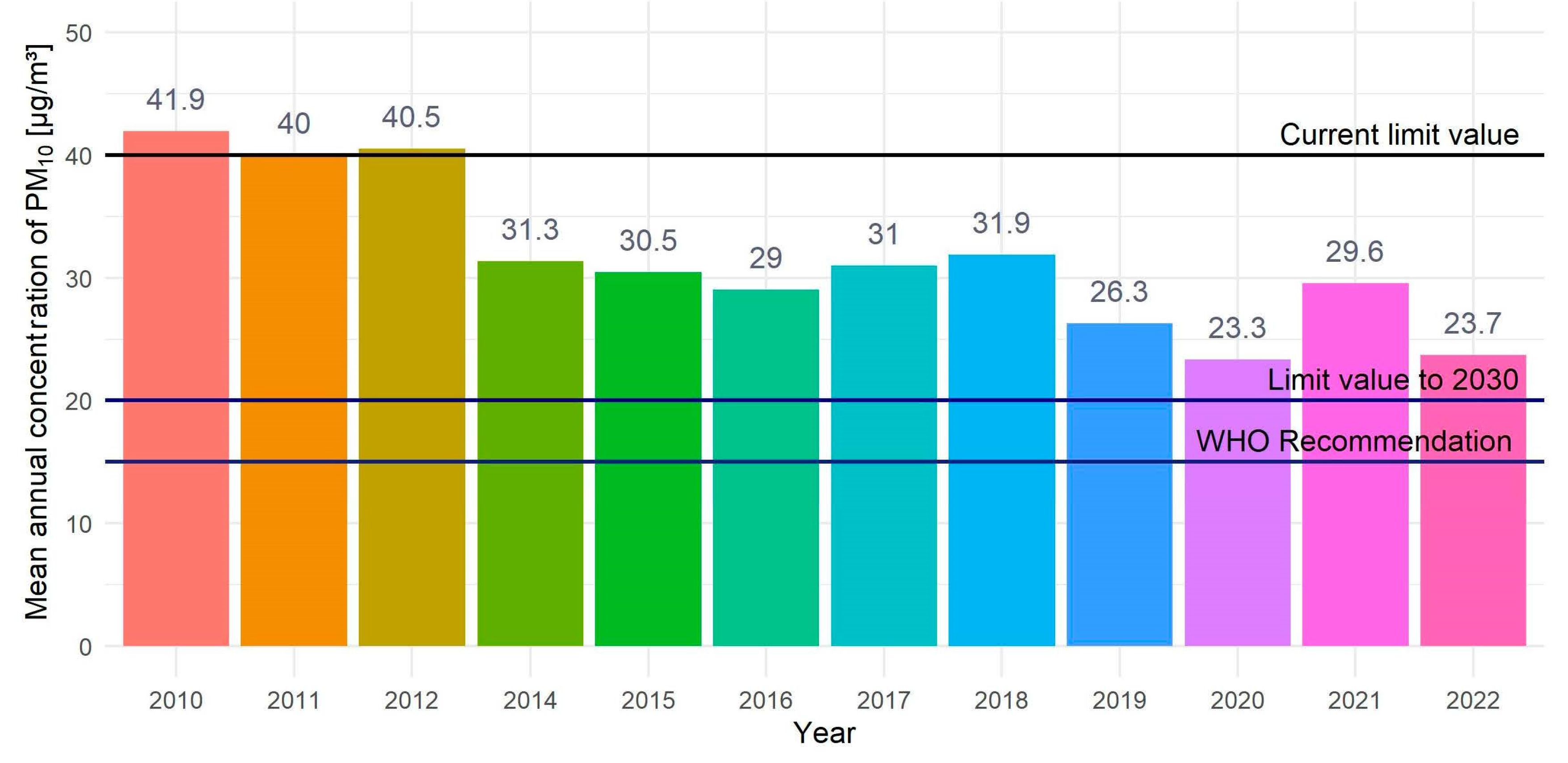
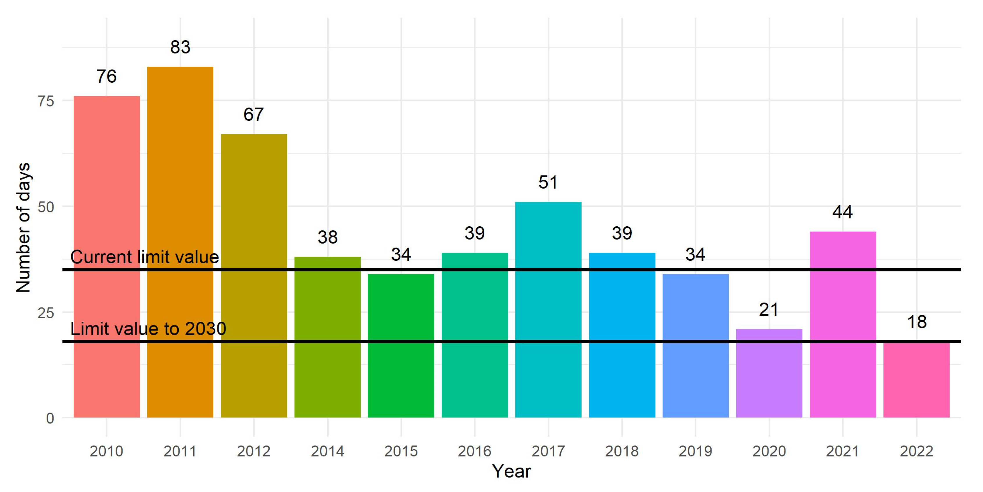
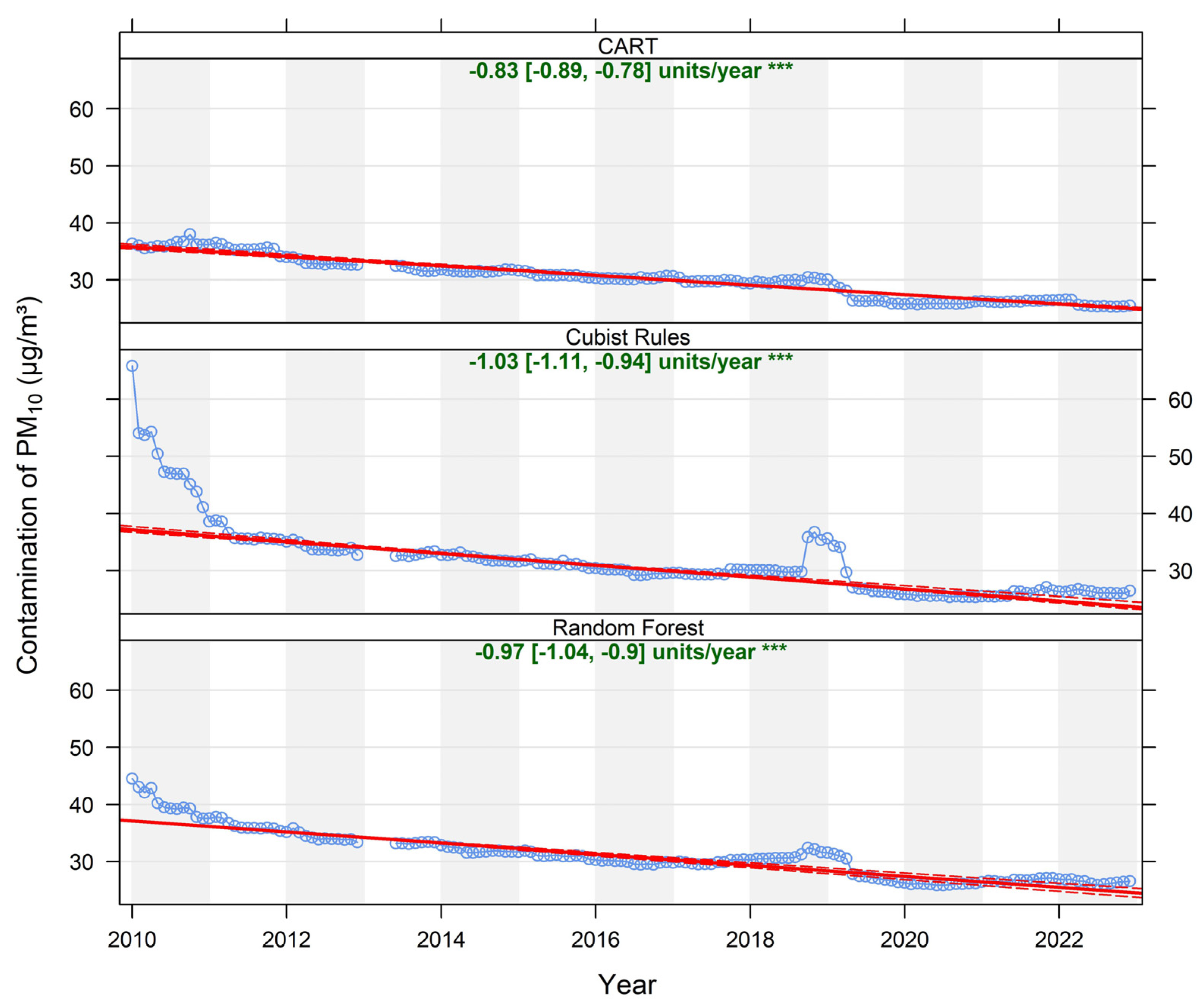
3.3. Comparison of Particulate Matter Trends

The results of PM10 concentration trends are presented in Figure 6. The solid red line shows the trend estimate and the dashed red lines show the 95% confidence intervals for the trend based on resampling methods. For CART, the trend is −0.83 (0.89–0.78) μg/m3, for Cubist, it is −1.03 (1.11–0.94) μg/m3, and for Ranger, it is −0.97 (1.04–0.9) μg/m3. The trend line for each model has a negative slope coefficient despite discrepancies in the accuracy assessment results (see Section 3.1). It should be noted that the 95% confidence intervals of the trend obtained from the Cubist and Ranger algorithms overlap. This indicates that they are not statistically significantly different at the 95% confidence level. Therefore, we can conclude that regardless of the applied algorithm (Ranger or Cubist), the differing importance of individual variables yields a similar trend value. Moving forward, when obtaining similar accuracy assessment results, a statistically comparable trend value is achieved. However, referring to the trend result obtained for the CART model, it was found to be statistically significantly different from the other algorithms. Furthermore, the mean value of the obtained trend was lower by approximately 0.14–0.20 μg/m3. This indicates that choosing the Decision Tree model, which is characterised by distinctly lower evaluation parameters, tends to underestimate the PM10 trend level.
The variability of monthly average normalised concentrations, presented in Figure 6, indicates that in the case of the CART model, it is not possible to detect interventions, thus limiting the application of the normalisation algorithm [9]. On the other hand, two distinct interventions were identified in the case of the other algorithms, where the Cubist model proved to be more sensitive. This suggests that it may be significantly more useful for identifying the effects of remedial actions introduced. Mallet (2021) [24] also conducted an analysis of PM10 concentration trends using the Random Forest model and the Gradient Boosted Regression Model. The results obtained from both models were very close (the difference was only 0.1 μg/m3) and accurately reflected actual data. Similarly to our research, they did not show statistically significant differences as their confidence intervals overlapped. This indicates that models with similar accuracy, but not necessarily consistent structures (e.g., in terms of variable importance), can yield statistically similar results in trend analysis.
The two distinct interventions mentioned (see Figure 6) occurred during the years 2010–2013 (a decrease in PM10 concentrations from approximately 45 μg/m3 in 2010 to 35 μg/m3 in 2013) and 2018–2019 (a marked temporary increase in PM10 concentrations from around 30 μg/m3 to 34 μg/m3). Between 2010 and 2012, road modernization and traffic improvements were carried out, including the construction of the Krzyż interchange on the A4 motorway. Additionally, in 2013, restrictions were introduced limiting the entry of trucks over 12 tons into the city centre. These actions are suspected to be the main remediation measures that contributed to the significant decline in PM10 concentrations. It is also important to note that this was not only caused by a reduction in emissions from road transport but also the completion of construction work at the Krzyż interchange. During these works, intensive earthworks took place, which may have caused an increase in PM10 concentrations due to secondary suspension of dusty material and wind erosion. The second detected intervention in 2018–2019 (a temporary increase in PM10 concentrations) was a consequence of significant road investments carried out during that period in the city of Tarnów, such as the modernization and reconstruction of Lwowska Street, Elektryczna Street, and Orkan Street. As mentioned, roadworks often involve variable activities that lead to the dispersion of dusty material onto the surfaces of many adjacent roads. Deposited material on neighbouring road surfaces is then resuspended by mechanical turbulence caused by passing vehicles [57,58,59]. In addition to the identified interventions, a steady downward trend in PM10 concentrations is observed, which is undoubtedly related to the systematic elimination of individual heating sources implemented under the “Clean Air” programme. This programme involved subsidising the replacement or removal of individual heating units. Typically, buildings were connected to district heating networks, new boilers meeting specified standards were installed, or alternative eco-friendly technologies were employed (heat pumps, solar collectors, photovoltaic panels). Between 2010 and 2022, over 2000 inefficient individual heating units were replaced or removed in Tarnów, accounting for approximately 50% of all inventoried low-emission sources.

4. Conclusions

The comparison of the three algorithms reveals that the Random Forest (Ranger) and Cubist Rules models achieved very similar accuracy in predicting PM10 concentrations. Ranger demonstrated a slightly higher Pearson correlation coefficient (0.89 vs. 0.88 for Cubist), while Cubist had a marginally lower RMSE (14.06 vs. 14.09 μg/m3). Both models had identical values for the coefficient of efficiency (0.52) and Willmott’s index of agreement (0.76). The CART model exhibited noticeably worse results across all metrics (RMSE: 19.96 μg/m3; COE: 0.33).
The variable importance analysis demonstrated that air temperature (tt) and boundary layer height (blh) were the most significant predictors across all models. Removing the temperature variable led to an increase in RMSE to over 20 μg/m3 (median: 23.9 for Ranger, 21.5 for Cubist, and 31.6 for CART), while removing blh resulted in an RMSE exceeding 19 μg/m3. Temporal variables, such as date and day of the year, also had a significant impact, whereas parameters like the day of the week or cloud base height proved to be of little importance.
Meteorological normalisation results demonstrated statistically significant downward PM10 trends across all models. The Cubist model indicated the largest average annual decrease (−1.03 μg/m3), while the CART model showed the smallest annual decrease (−0.83 μg/m3). It is important to note that the confidence intervals for Cubist and Ranger overlapped, signifying no significant difference between these models. The Cubist model proved particularly effective in identifying the impact of political interventions on air quality.
Detailed conclusions regarding the evaluation of the algorithms, variable importance analysis, and trend value comparisons clearly indicate that the Random Forest and Cubist Rules algorithms should be considered appropriate and equivalent tools for use in the meteorological normalisation of PM10 concentrations. In contrast, the use of the Decision Tree algorithm is not recommended due to its significantly lower predictive accuracy and statistically significant differences in PM10 concentration trend values at the 95% confidence level. For operational monitoring applications aimed at identifying implemented mitigation actions, we recommend using the Random Forest algorithm, as the model training process is approximately 6 to 10 times faster than that of Cubist Rules, depending on the complexity of the input dataset.
It should be emphasised, however, that the proposed solution is representative only for a specific location and the analysed pollutant, as it does not take into account information regarding emission volumes or orographic conditions. Therefore, any change in location or pollutant type requires redeveloping the model based on the available dataset. A significant advantage of the applied technique, compared to classical air pollution dispersion modelling methods [47,48], is the high accuracy of the obtained results and the considerably lower effort required for preparing input data.
Despite the observed improvement in air quality (a 43.4% reduction in PM10 concentrations between 2010 and 2022), the annual average concentrations in Tarnów still exceed both WHO guidelines (15 μg/m3) and the new EU standards (20 μg/m3). These results emphasise the need for further remedial actions in air protection. This demonstrates that municipal interventions, such as emission reduction programmes aimed at achieving the required air quality standards, are yielding benefits. While air quality in Tarnów is improving, continued mobilisation by the local government and residents is essential to strive for the achievement of the new lower permissible PM10 concentration levels and other air pollution standards established by the European Parliament and the Council of the European Union.

Supplementary Materials

The following supporting information can be downloaded at: https://www.mdpi.com/article/10.3390/su17125274/s1, Table S1: Measurement dataset used in the study and results of calculations of normalized PM10 concentration.

Author Contributions

Conceptualization, M.R.; methodology, M.R.; software, K.G.; validation, K.G.; formal analysis, M.R. and K.G.; investigation, M.R. and K.G.; resources, M.R. and K.G.; data curation, K.G.; writing—original draft preparation, M.R. and K.G.; writing—review and editing, M.R. and K.G.; visualisation, K.G.; supervision, M.R.; project administration, M.R.; funding acquisition, M.R. All authors have read and agreed to the published version of the manuscript.

Funding

The work was carried out as part of research associated with the Ministry of Science and Higher Education (Poland) subsidy for AGH University of Krakow to maintain scientific potential (Contract no. 16.16.150.545) and “Excellence initiative—research university” programme for AGH University of Krakow.

Institutional Review Board Statement

Not applicable.

Informed Consent Statement

Not applicable.

Data Availability Statement

The datasets of this study are not publicly available. However, they may be made available upon reasonable request by the author.

Conflicts of Interest

The authors declare no conflicts of interest.

Abbreviations

The following abbreviations are used in this manuscript:
EUEuropean Union
WHOWorld Health Organization
PM10Particulate matter
NOxNitrogen oxide
NO2Nitrogen dioxide
SO2Sulfur dioxide
COCarbon monoxide
O3Ozone
RFRandom Forest
GBMGradient Boosted Regression Model
wsWind speed
wd_cutWind direction
rhRelative humidity
ttAir temperature
presAtmospheric pressure
blhBoundary layer height
cbhCloud base height
ssrSurface net solar radiation
CARTDecision Tree Model
RangerRandom Forest Model
CubistCubist Rules Model
jdayDay of the year according to the Julian calendar
wdayDay of the week
hourHour of the day
FAC2Fraction of predictions within a factor of two
MBThe mean bias
MGEThe mean gross error
NMBThe normalised mean bias
NMGEThe normalised mean gross error
RMSEThe root mean square error
rThe Pearson correlation coefficient
COEThe coefficient of efficiency
IOAThe Index of Agreement based on Willmott
R2The coefficient of determination
EMAExploratory Model Analysis

Appendix A

Figure A1. Spearman correlation matrix between the analysed independent variables and the dependent variable.
Sustainability 17 05274 g0a1
Table A1. Tabular summary and description of statistical metrics used for model evaluation.
IndicatorFull NameDescription
FAC2Fraction of predictions within a factor of twoPercentage of predictions within the range of 0.5 to 2 times the observed value.
MBMean BiasAverage difference between predicted and observed values.
MGEMean Gross ErrorAverage absolute difference between predicted and observed values.
NMBNormalised Mean BiasMean Bias divided by the sum of observed values, expressed as a percentage.
NMGENormalised Mean Gross ErrorMean Gross Error divided by the sum of observed values, expressed as a percentage.
RMSERoot Mean Square ErrorError measure that gives greater weight to large deviations.
rPearson Correlation CoefficientMeasures the strength of the linear relationship between observed and predicted values.
COECoefficient of EfficiencyIndicates how well the model predictions match observed values.
IOAIndex of AgreementMeasures the degree of model agreement with observations.

References

  1. Loomis, D.; Grosse, Y.; Lauby-Secretan, B.; El Ghissassi, F.; Bouvard, V.; Benbrahim-Tallaa, L.; Guha, N.; Baan, R.; Mattock, H.; Straif, K. The Carcinogenicity of Outdoor Air Pollution. Lancet Oncol. 2013, 14, 1262–1263. [Google Scholar] [CrossRef]
  2. Zhang, Y.; Ma, Y.; Feng, F.; Cheng, B.; Wang, H.; Shen, J.; Jiao, H. Association between PM10 and Specific Circulatory System Diseases in China. Sci. Rep. 2021, 11, 12129. [Google Scholar] [CrossRef]
  3. Combes, A.; Franchineau, G. Fine Particle Environmental Pollution and Cardiovascular Diseases. Metabolism 2019, 100, 153944. [Google Scholar] [CrossRef]
  4. Caffè, A.; Scarica, V.; Animati, F.M.; Manzato, M.; Bonanni, A.; Montone, R.A. Air Pollution and Coronary Atherosclerosis. Future Cardiol. 2025, 21, 53–66. [Google Scholar] [CrossRef]
  5. Basith, S.; Manavalan, B.; Shin, T.H.; Park, C.B.; Lee, W.S.; Kim, J.; Lee, G. The Impact of Fine Particulate Matter 2.5 on the Cardiovascular System: A Review of the Invisible Killer. Nanomaterials 2022, 12, 2656. [Google Scholar] [CrossRef]
  6. International Agency for Research on Cancer. Air Pollution and Cancer; Straif, K., Cohen, A., Samet, J., Eds.; IARC Scientific Publications: Lyon, France, 2013; Volume 161, ISBN 978-92-832-2. [Google Scholar]
  7. European Environment Agency. Air Quality in Europe 2022; European Environment Agency: Copenhagen, Denmark, 2022. [Google Scholar]
  8. Cakaj, A.; Lisiak-Zielińska, M.; Khaniabadi, Y.O.; Sicard, P. Premature Deaths Related to Urban Air Pollution in Poland. Atmos. Environ. 2023, 301, 119723. [Google Scholar] [CrossRef]
  9. Grange, S.K.; Carslaw, D.C. Using Meteorological Normalisation to Detect Interventions in Air Quality Time Series. Sci. Total Environ. 2019, 653, 578–588. [Google Scholar] [CrossRef]
  10. Grange, S.K.; Carslaw, D.C.; Lewis, A.C.; Boleti, E.; Hueglin, C. Random Forest Meteorological Normalisation Models for Swiss PM 10 Trend Analysis. Atmos. Chem. Phys. 2018, 18, 6223–6239. [Google Scholar] [CrossRef]
  11. Vu, T.V.; Shi, Z.; Cheng, J.; Zhang, Q.; He, K.; Wang, S.; Harrison, R.M. Assessing the Impact of Clean Air Action on Air Quality Trends in Beijing Using a Machine Learning Technique. Atmos. Chem. Phys. 2019, 19, 11303–11314. [Google Scholar] [CrossRef]
  12. Ceballos-Santos, S.; González-Pardo, J.; Carslaw, D.C.; Santurtún, A.; Santibáñez, M.; Fernández-Olmo, I. Meteorological Normalisation Using Boosted Regression Trees to Estimate the Impact of COVID-19 Restrictions on Air Quality Levels. Int. J. Environ. Res. Public Health 2021, 18, 13347. [Google Scholar] [CrossRef]
  13. Lovrić, M.; Antunović, M.; Šunić, I.; Vuković, M.; Kecorius, S.; Kröll, M.; Bešlić, I.; Godec, R.; Pehnec, G.; Geiger, B.C.; et al. Machine Learning and Meteorological Normalization for Assessment of Particulate Matter Changes during the COVID-19 Lockdown in Zagreb, Croatia. Int. J. Environ. Res. Public Health 2022, 19, 6937. [Google Scholar] [CrossRef]
  14. Munir, S.; Coskuner, G.; Jassim, M.S.; Aina, Y.A.; Ali, A.; Mayfield, M. Changes in Air Quality Associated with Mobility Trends and Meteorological Conditions during COVID-19 Lockdown in Northern England, UK. Atmosphere 2021, 12, 504. [Google Scholar] [CrossRef]
  15. Petetin, H.; Bowdalo, D.; Soret, A.; Guevara, M.; Jorba, O.; Serradell, K.; Pérez García-Pando, C. Meteorology-Normalized Impact of the COVID-19 Lockdown upon NO2 Pollution in Spain. Atmos. Chem. Phys. 2020, 20, 11119–11141. [Google Scholar] [CrossRef]
  16. Lv, Y.; Tian, H.; Luo, L.; Liu, S.; Bai, X.; Zhao, H.; Lin, S.; Zhao, S.; Guo, Z.; Xiao, Y.; et al. Meteorology-Normalized Variations of Air Quality during the COVID-19 Lockdown in Three Chinese Megacities. Atmos. Pollut. Res. 2022, 13, 101452. [Google Scholar] [CrossRef]
  17. Gagliardi, R.V.; Andenna, C. Machine Learning Meteorological Normalization Models for Trend Analysis of Air Quality Time Series. Int. J. Environ. Impacts 2021, 4, 375–387. [Google Scholar] [CrossRef]
  18. Falocchi, M.; Zardi, D.; Giovannini, L. Meteorological Normalization of NO2 Concentrations in the Province of Bolzano (Italian Alps). Atmos. Environ. 2021, 246, 118048. [Google Scholar] [CrossRef]
  19. Zheng, H.; Kong, S.; Zhai, S.; Sun, X.; Cheng, Y.; Yao, L.; Song, C.; Zheng, Z.; Shi, Z.; Harrison, R.M. An Intercomparison of Weather Normalization of PM2.5 Concentration Using Traditional Statistical Methods, Machine Learning, and Chemistry Transport Models. NPJ Clim. Atmos. Sci. 2023, 6, 214. [Google Scholar] [CrossRef]
  20. Ali-Taleshi, M.S.; Riyahi Bakhtiari, A.; Hopke, P.K. Meteorologically Normalized Spatial and Temporal Variations Investigation Using a Machine Learning-Random Forest Model in Criteria Pollutants across Tehran, Iran. Urban Clim. 2024, 53, 101790. [Google Scholar] [CrossRef]
  21. Kamińska, J.A. A Random Forest Partition Model for Predicting NO2 Concentrations from Traffic Flow and Meteorological Conditions. Sci. Total Environ. 2019, 651, 475–483. [Google Scholar] [CrossRef]
  22. Kamińska, J.A. The Use of Random Forests in Modelling Short-Term Air Pollution Effects Based on Traffic and Meteorological Conditions: A Case Study in Wrocław. J. Environ. Manag. 2018, 217, 164–174. [Google Scholar] [CrossRef]
  23. Cole, M.A.; Elliott, R.J.R.; Liu, B. The Impact of the Wuhan COVID-19 Lockdown on Air Pollution and Health: A Machine Learning and Augmented Synthetic Control Approach. Environ. Resour. Econ. 2020, 76, 553–580. [Google Scholar] [CrossRef]
  24. Mallet, M.D. Meteorological Normalisation of PM10 Using Machine Learning Reveals Distinct Increases of Nearby Source Emissions in the Australian Mining Town of Moranbah. Atmos. Pollut. Res. 2021, 12, 23–35. [Google Scholar] [CrossRef]
  25. Wu, Q.; Li, T.; Zhang, S.; Fu, J.; Seyler, B.C.; Zhou, Z.; Deng, X.; Wang, B.; Zhan, Y. Evaluation of NOx Emissions before, during, and after the COVID-19 Lockdowns in China: A Comparison of Meteorological Normalization Methods. Atmos. Environ. 2022, 278, 119083. [Google Scholar] [CrossRef]
  26. Quinlan, J.R. Combining Instance-Based and Model-Based Learning. In Proceedings of the International Conference on Machine Learning 1993, Amherst, MA, USA, 27–29 June 1993; pp. 236–243. [Google Scholar] [CrossRef]
  27. Kuhn, M.; Johnson, K. Applied Predictive Modeling; Springer: Berlin/Heidelberg, Germany, 2013; pp. 1–600. [Google Scholar] [CrossRef]
  28. Zhang, G.; Lu, H.; Dong, J.; Poslad, S.; Li, R.; Zhang, X.; Rui, X. A Framework to Predict High-Resolution Spatiotemporal PM2.5 Distributions Using a Deep-Learning Model: A Case Study of Shijiazhuang, China. Remote Sens. 2020, 12, 2825. [Google Scholar] [CrossRef]
  29. Xu, Y.; Ho, H.C.; Wong, M.S.; Deng, C.; Shi, Y.; Chan, T.C.; Knudby, A. Evaluation of Machine Learning Techniques with Multiple Remote Sensing Datasets in Estimating Monthly Concentrations of Ground-Level PM2.5. Environ. Pollut. 2018, 242, 1417–1426. [Google Scholar] [CrossRef]
  30. Walsh, K.J.; Milligan, M.; Woodman, M.; Sherwell, J. Data Mining to Characterize Ozone Behavior in Baltimore and Washington, DC. Atmos. Environ. 2008, 42, 4280–4292. [Google Scholar] [CrossRef]
  31. Magesh, S.; Geng, K. A Machine Learning Interpretation of the Correlation between Poverty and Air Pollution in the Contiguous United States. Sci. Rep. 2025, 15, 2407. [Google Scholar] [CrossRef]
  32. Méndez, M.; Merayo, M.G.; Núñez, M. Machine Learning Algorithms to Forecast Air Quality: A Survey. Artif. Intell. Rev. 2023, 56, 10031–10066. [Google Scholar] [CrossRef]
  33. Tian, H.; Huang, L.; Hu, S.; Wu, W. A Modified Machine Learning Algorithm for Multi-Collinearity Environmental Data. Environ. Ecol. Stat. 2024, 31, 1063–1083. [Google Scholar] [CrossRef]
  34. Mampitiya, L.; Rathnayake, N.; Hoshino, Y.; Rathnayake, U. Performance of Machine Learning Models to Forecast PM10 Levels. MethodsX 2024, 12, 102557. [Google Scholar] [CrossRef]
  35. European Parliament; The Council of the European Union. Directive (EU) 2024/2881 of the European Parliament and of the Council of 23 October 2024 on Ambient Air Quality and Cleaner Air for Europe. Off. J. Eur. Union 2024, L 2881, 1–30. [Google Scholar]
  36. Chief Inspectorate of Environmental Protection (GIOS). Air Quality Monitoring Archive; Chief Inspectorate of Environmental Protection (GIOS): Warsaw, Poland, 2025. [Google Scholar]
  37. Institute of Meteorology; (IMGW-PIB), W.M. Public Data Portal 2025. Available online: https://danepubliczne.imgw.pl/ (accessed on 20 May 2024).
  38. Hersbach, H.; Bell, B.; Berrisford, P.; Biavati, G.; Horányi, A.; Muñoz Sabater, J.; Nicolas, J.; Peubey, C.; Radu, R.; Rozum, I.; et al. ERA5 Hourly Data on Single Levels from 1979 to Present; European Centre for Medium-Range Weather Forecasts: Reading, UK, 2023. [Google Scholar]
  39. Rokach, L.; Maimon, O. Decision Trees. In Data Mining and Knowledge Discovery Handbook; Rokach, L., Maimon, O., Eds.; Springer: Boston, MA, USA, 2005; pp. 165–192. ISBN 038725465X. [Google Scholar]
  40. Breiman, L. Random Forests. Mach. Learn. 2001, 45, 5–32. [Google Scholar] [CrossRef]
  41. Wright, M.N.; Ziegler, A. Ranger: A Fast Implementation of Random Forests for High Dimensional Data in C++ and R. J. Stat. Softw. 2017, 77, 1–17. [Google Scholar] [CrossRef]
  42. Kuhn, M.; Wickham, H. Tidymodels: A Collection of Packages for Modeling and Machine Learning Using Tidyverse Principles. Available online: https://www.tidymodels.org (accessed on 20 May 2024).
  43. Carslaw, D.C.; Ropkins, K. Openair—An r Package for Air Quality Data Analysis. Environ. Model. Softw. 2012, 27–28, 52–61. [Google Scholar] [CrossRef]
  44. Biecek, P.; Burzykowski, T. Explanatory Model Analysis; Chapman and Hall/CRC: New York, NY, USA, 2021; ISBN 9780367135591. [Google Scholar]
  45. Kunsch, H.R. Annals of Statistics. Jackknife Bootstrap Gen. Station. Obs. 1989, 17, 1217–1241. [Google Scholar]
  46. Wang, X.; Yu, Q. Unbiasedness of the Theil–Sen Estimator. J. Nonparametr. Stat. 2005, 17, 685–695. [Google Scholar] [CrossRef]
  47. Rzeszutek, M. Parameterization and Evaluation of the CALMET/CALPUFF Model System in near-Field and Complex Terrain—Terrain Data, Grid Resolution and Terrain Adjustment Method. Sci. Total Environ. 2019, 689, 31–46. [Google Scholar] [CrossRef]
  48. Rzeszutek, M.; Szulecka, A. Assessment of the AERMOD Dispersion Model in Complex Terrain with Different Types of Digital Elevation Data. IOP Conf. Ser. Earth Environ. Sci. 2021, 642, 012014. [Google Scholar] [CrossRef]
  49. Rood, A.S. Performance Evaluation of AERMOD, CALPUFF, and Legacy Air Dispersion Models Using the Winter Validation Tracer Study Dataset. Atmos. Environ. 2014, 89, 707–720. [Google Scholar] [CrossRef]
  50. Carruthers, D.J.; Seaton, M.D.; McHugh, C.A.; Sheng, X.; Solazzo, E.; Vanvyve, E. Comparison of the Complex Terrain Algorithms Incorporated into Two Commonly Used Local-Scale Air Pollution Dispersion Models (ADMS and AERMOD) Using a Hybrid Model. J. Air Waste Manag. Assoc. 2011, 61, 1227–1235. [Google Scholar] [CrossRef]
  51. Thepanondh, S.; Jittra, N.; Pinthong, N. Performance Evaluation of AERMOD and CALPUFF Air Dispersion Models in Industrial Complex Area. Air Soil Water Res. 2015, 8, 87–95. [Google Scholar] [CrossRef]
  52. Biecek, P. DALEX: Explainers for Complex Predictive Models in R. J. Mach. Learn. Res. 2018, 19, 1–5. [Google Scholar]
  53. Szulecka, A.; Oleniacz, R.; Rzeszutek, M. Functionality of Openair Package in Air Pollution Assessment and Modeling—A Case Study of Krakow. Environ. Prot. Nat. Resour. 2017, 28, 22–27. [Google Scholar] [CrossRef]
  54. Oleniacz, R.; Bogacki, M.; Szulecka, A.; Rzeszutek, M.; Mazur, M. Assessing the Impact of Wind Speed and Mixing-Layer Height on Air Quality in Krakow (Poland) in the Years 2014–2015. J. Civ. Eng. Environ. Archit. 2016, XXXIII, 315–342. [Google Scholar] [CrossRef]
  55. Foskinis, R.; Gini, M.I.; Kokkalis, P.; Diapouli, E.; Vratolis, S.; Granakis, K.; Zografou, O.; Komppula, M.; Vakkari, V.; Nenes, A.; et al. On the Relation between the Planetary Boundary Layer Height and in Situ Surface Observations of Atmospheric Aerosol Pollutants during Spring in an Urban Area. Atmos. Res. 2024, 308, 107543. [Google Scholar] [CrossRef]
  56. Du, C.; Liu, S.; Yu, X.; Li, X.; Chen, C.; Peng, Y.; Dong, Y.; Dong, Z.; Wang, F. Urban Boundary Layer Height Characteristics and Relationship with Particulate Matter Mass Concentrations in Xi’an, Central China. Aerosol Air Qual. Res. 2013, 13, 1598–1607. [Google Scholar] [CrossRef]
  57. Bogacki, M.; Oleniacz, R.; Rzeszutek, M.; Paulina, B.; Szulecka, A. Assessing the Impact of Road Traffic Reorganization on Air Quality: A Street Canyon Case Study. Atmosphere 2020, 11, 695. [Google Scholar] [CrossRef]
  58. Bogacki, M.; Mazur, M.; Oleniacz, R.; Rzeszutek, M.; Szulecka, A. Re-Entrained Road Dust PM10 Emission from Selected Streets of Krakow and Its Impact on Air Quality. E3S Web Conf. 2018, 28, 01003. [Google Scholar] [CrossRef]
  59. Rzeszutek, M.; Bogacki, M.; Paulina, B.; Szulecka, A. Improvement Assessment of the OSPM Model Performance by Considering the Secondary Road Dust Emissions. Transp. Res. Part D Transp. Environ. 2019, 68, 137–149. [Google Scholar] [CrossRef]
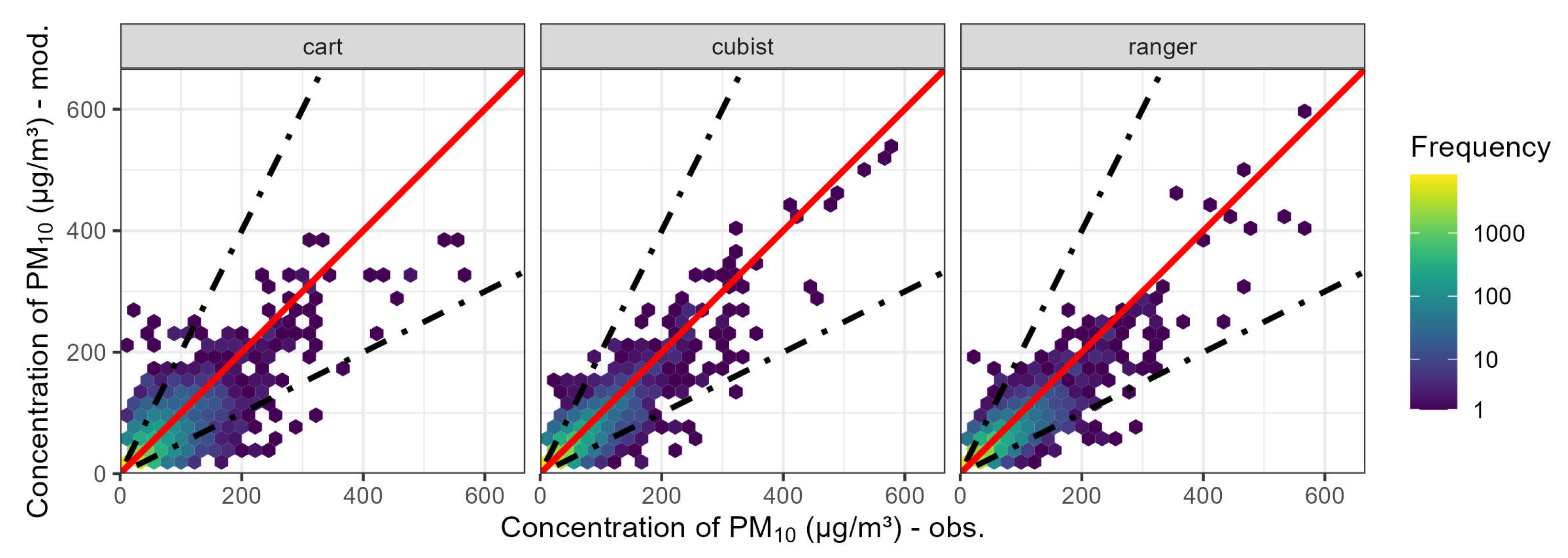
Figure 1. Graphical representation of the study area and the locations of meteorological and air quality monitoring stations.
Sustainability 17 05274 g001
Figure 2. Comparison of average annual PM10 concentrations from air quality monitoring stations in Tarnów against different air quality standards (current limit value, limit value for 2030, WHO recommendation).
Sustainability 17 05274 g002
Figure 3. Distribution of days per year when the daily average PM10 air quality standard was exceeded in Tarnów.
Sustainability 17 05274 g003
Figure 4. Scatterplot of the comparison of PM10 observations with modelling results on the test dataset for three machine learning algorithms (red line—ideal model; black line—double overestimation or underestimation).
Sustainability 17 05274 g004
Figure 5. Comparison of predictor variable importance across three machine learning models (CART, Cubist Rules, and Random Forest) based on RMSE variation after variable permutation.
Sustainability 17 05274 g005
Figure 6. Graphical representation of the PM10 concentration trend with 95% confidence intervals, determined using three machine learning algorithms (***—p-value < 0.001, very strong evidence of a trend; blue circle—monthly mean normalized PM10 concentrations (µg/m3).
Sustainability 17 05274 g006
Table 1. Summary of model accuracy metrics depending on the supervised learning algorithm used.
ModelFAC2MBMGENMBNMGERMSErCOEIOA
Cart0.82−0.1411.94−0.0010.3919.960.750.330.66
Cubist0.90−0.118.52−0.0400.2814.060.880.520.76
Ranger0.910.118.460.0040.2814.090.890.520.76
Disclaimer/Publisher’s Note: The statements, opinions and data contained in all publications are solely those of the individual author(s) and contributor(s) and not of MDPI and/or the editor(s). MDPI and/or the editor(s) disclaim responsibility for any injury to people or property resulting from any ideas, methods, instructions or products referred to in the content.

