Immune-Inspired Multi-Objective PSO Algorithm for Optimizing Underground Logistics Network Layout with Uncertainties: Beijing Case Study

Abstract

With the rapid acceleration of global urbanization and the advent of smart city initiatives, large metropolises confront the dual challenges of surging logistics demand and constrained surface transportation resources. Traditional surface logistics networks struggle to support sustainable urban development in high-density areas due to traffic congestion, high carbon emissions, and inefficient last-mile delivery. This paper addresses the layout optimization of a hub-and-spoke underground space logistics system (ULS) network for smart cities under stochastic scenarios by proposing an immune-inspired multi-objective particle swarm optimization (IS-MPSO) algorithm. By integrating a stochastic robust Capacity–Location–Allocation–Routing (CLAR) model, the approach concurrently minimizes construction costs, maximizes operational efficiency, and enhances underground corridor load rates while embedding probability density functions to capture multidimensional uncertainty parameters. Case studies in Beijing’s Fifth Ring area demonstrate that the IS-MPSO algorithm reduces the total objective function value from 9.8 million to 3.4 million within 500 iterations, achieving stable convergence in an average of 280 iterations. The optimized ULS network adopts a “ring–synapse” topology, elevating the underground corridor load rate to 59% and achieving a road freight alleviation rate (RFAR) of 98.1%, thereby shortening the last-mile delivery distance to 1.1 km. This research offers a decision-making paradigm that balances economic efficiency and robustness for the planning of underground logistics space in smart cities, contributing to the sustainable urban development of high-density regions and validating the algorithm’s effectiveness in large-scale combinatorial optimization problems.

1. Introduction

With the rapid acceleration of global urbanization and the rise of smart city initiatives, mega-cities are confronting the dual challenges of surging logistics demand and severely constrained surface transportation resources. Traditional surface logistics networks—hampered by chronic traffic congestion, elevated carbon emissions, and inefficient last-mile delivery—are increasingly inadequate for supporting the sustainable urban development of high-density agglomerations [1]. Against this backdrop, the underground logistics system (ULS), leveraging underutilized underground space, has emerged as an innovative infrastructure solution that aligns with both smart city objectives and sustainable urban development goals [2,3]. By shifting freight flows into subterranean corridors, ULSs not only relieve surface traffic pressure and curb environmental pollution but also bolster the resilience and emergency response capabilities of urban logistics networks [4,5,6]. In particular, a hub-and-spoke topology within the ULS framework—characterized by streamlined connectivity and high levels of resource consolidation—has become a cornerstone paradigm in planning underground space logistics for future-ready smart cities [5,7].

Currently, most ULS network optimization studies have prioritized single-objective cost minimization under deterministic settings, as typified by [2,8]. Such approaches, however, fall short of capturing the stochastic uncertainties intrinsic to real-world engineering—ranging from volatile demand patterns and dynamic facility capacities to complex subsurface geographic constraints [9,10]. Moreover, conventional multi-objective algorithms like NSGA-II frequently become trapped in local optima when addressing ultra-large-scale problems with high-dimensional decision variables, thereby compromising the balance between convergence and solution diversity [11]. Consequently, there is an urgent need for a robust, multi-objective modeling framework that concurrently optimizes construction expenditure, operational performance, and resource utilization within the stochastic underground environment of a sustainable smart city.

On the theoretical front, the existing literature has not systematically explored robust multi-objective optimization for ULS networks [12,13,14]. For example, robust facility location models overlook interaction effects across facility hierarchies [15], while deterministic planning methodologies cannot accommodate real demand variability [16]. To bridge these gaps, this paper pioneers the incorporation of multidimensional uncertainty parameters—such as origin–destination demand distributions and construction cost fluctuations—into a hub-and-spoke network optimization model via probability density functions and cumulative distribution transformations. This advancement not only fills a critical theoretical void in stochastic robust modeling for underground space logistics, but also resonates with the imperatives of sustainable urban development and dual-carbon targets in China’s mega-cities, where land for logistics is at a premium.

In terms of methodological innovation and practical contributions, this paper develops a stochastic robust multi-objective Capacity–Location–Allocation–Routing (CLAR) integrated model that achieves the coordinated optimization of facility construction costs, corridor load factors, and operational efficiency. The model’s complexity is significantly higher than that of traditional two-echelon facility location problems (2E-CFLAPs), thereby reflecting a greater level of engineering realism. To address the challenges posed by ultra-large-scale combinatorial optimization, an immune-inspired multi-objective particle swarm optimization algorithm (IS-MPSO) is also proposed. By incorporating an immune selection mechanism and dynamic search strategies, the algorithm effectively enhances global search capabilities and increases the diversity of the Pareto front. A detailed case study of Beijing’s Fifth Ring area validates the practical applicability of our framework, demonstrating how ULS network topologies can dynamically adapt to stochastic demand and providing a novel decision-support paradigm for underground space logistics planning in sustainable, smart urban environments.

The paper is structured as follows: In Section 2, a comprehensive review of ULS network topology paradigms and recent advances in stochastic optimization is presented. Section 3 details the development of the stochastic robust CLAR model, while Section 4 elaborates on the solution methodologies employed. Section 5 discusses simulation results based on a case study in Beijing’s Fifth Ring Road area. Finally, Section 6 concludes the paper by summarizing the findings and outlining prospects for future research directions and policy recommendations.

2. Research Background

2.1. Knowledge of ULS Studies

2.1.1. Planning of ULS Networks

The earliest freight pipeline system emerged in London (1853), where the mail was delivered between stock exchanges in pneumatic tubes [17]. Other early ULSs include the first mail pipeline network built in Berlin (1865), the Chicago underground parcel distribution system in 1906, and the Tub express supply system in the Soviet Union [17]. Most of those systems were planned as short-haul, single-line, single-purpose, and enclosed, only serving as a kind of point-to-point transport means rather than a complete logistics system.

The concept of a modern ULS was generally proposed in [18], where it was formally defined as an advanced underground transportation technology for moving a variety of solid commodities. Since then, many ULS initiatives have been issued around the world. One of the most popular applications is to build local ULS channels inside a logistics gateway to facilitate logistics operations. Representative case studies and pilot projects have taken place in Port of Antwerp [19], Port of Shanghai [16,20] and Amsterdam airport [21]. Another popular application is to build several ULS lines to transport homogeneous containers and freight pallets among gateways, urban logistics parks, and inner-city logistics centers [16,21,22]. In the future, dedicated tunnels might be considered for the use of demolition waste collection [23,24].

A review of ULS development reveals a shift towards a more complex underground network layouts. Large-scale feasibility planning methods for underground pipeline networks have become essential decision-support tools and have gained increasing attention from researchers. For instance, ref. [25] proposed an effective modeling and optimization approach for ULS network planning in urban areas, specifically for a hub-and-spoke ULS configuration. They formulated a mixed-integer programming model to minimize system costs and designed an algorithm for its solution. As research has progressed, multi-objective optimization problems have received increasing attention. Ref. [26] introduced an integrated design and facility planning method for a two-tier urban ULS hub-and-spoke network. They developed a bi-objective mixed-integer linear programming model that minimized cost while maximizing system utilization, employing a hybrid optimization approach that integrated exact and metaheuristic algorithms, with case-based simulations validating its effectiveness. Further advancing the field, ref. [27] designed a prototype for an integrated ULS encompassing network topology, facility operations, handling processes, and transportation parameters. They formulated a bi-objective dynamic programming model that incorporated multi-period network expansion mechanisms and developed a hybrid optimization algorithm that combined variable neighborhood search-based memetic algorithms, Kruskal’s minimum spanning tree algorithm, and the A-star algorithm.

The aforementioned studies indicate that mixed-integer programming (MIP) models have been widely applied to address various network optimization problems in ULS research [28,29,30,31]. Notably, MIP is a deterministic approach that assumes no randomness or uncertainty in the system [32,33]. However, ULS projects are inherently unpredictable and high-risk [34]. To better simulate real-world scenarios, stochastic elements must be incorporated into the models. Existing studies often consider only a single source of uncertainty (e.g., demand or cost), overlooking the interactions among multiple stochastic parameters [35]. Furthermore, most studies focus on bi-objective optimization, while integrating additional objectives—such as transportation efficiency and load cost—remains crucial [36,37].

Furthermore, bio-inspired algorithms—renowned for their strong global search capabilities and flexible multi-objective optimization mechanisms—have been widely applied to urban logistics and network planning. Representative methods include artificial immune systems (AISs), ant colony optimization (ACO), genetic algorithms (GAs), enhanced variants of particle swarm optimization (PSO), and other emerging approaches (e.g., the firefly algorithm and gray wolf optimizer) which have shown preliminary use in addressing urban logistics network problems [38]. AISs utilize an antibody–antigen interaction mechanism to adaptively adjust delivery routes, thereby effectively avoiding local optima in complex road networks [39]. ACO relies on pheromone evaporation and reinforcement dynamics to balance time-window constraints and capacity allocation in multi-objective logistics scheduling [38]. Enhanced PSO incorporates adaptive inertia weights and chaotic mapping schemes to significantly improve convergence stability in stochastic environments [32]. In addition to bio-inspired frameworks, a variety of stochastic and robust optimization techniques have been employed in logistics network planning. Examples include scenario-based stochastic programming, chance-constrained models, distributionally robust optimization, and adaptive robust methods [11,39].

To address these gaps, this study incorporates uncertainty in stochastic parameters while optimizing the ULS network with an integrated objective that includes transportation efficiency. Additionally, we propose an immune-inspired multi-objective PSO (IS-MPSO) algorithm, embedding stochastic robustness, dynamic search strategies, and immune mechanisms to enhance network optimization more effectively and realistically.

2.1.2. Key Technologies for ULSs

Urban ULSs draw on prototyping technologies mostly from underground engineering, vehicle and transportation engineering, logistics engineering, information science, and other fields. Most of these technologies have already been demonstrated in real-world applications [22].

(1) Pipeline conveyance and capsule vehicles.

ULS networks commonly employ closed-pipe conveyance systems paired with capsule vehicles that travel via pneumatic or magnetic-levitation guidance. The pipe material (e.g., steel or reinforced concrete) must ensure airtightness under pressures of 0.1–0.2 MPa, and capsule diameters typically range from 100 mm to 300 mm to accommodate parcels of up to 20 kg.

(2) Automated handling and sorting systems.

At hub nodes, automated guided vehicles (AGVs) equipped with LiDAR navigation shuttle capsules between storage racks and transfer points. Vertical lifting is achieved via high-speed belt conveyors or vertical carousels. Sorting employs RFID/barcode scanners and multidirectional sorters capable of 2000 parcels per hour.

(3) Integrated monitoring and dispatch platforms.

A centralized command center merges platform-collected data on pipeline pressure, capsule speed, AGV locations, and temperature/humidity into a GIS-BIM interface for real-time visualization. Dispatch algorithms combine genetic algorithms with particle swarm routines to balance throughput, energy consumption, and equipment load, re-optimizing paths every 5 min under dynamic demand.

(4) Safety and maintenance technologies.

Ventilation relies on variable-air-volume systems, and fire protection uses sectional fire dampers, smoke sensors, and a rapid-response sprinkler network.

2.2. Topological Paradigm and Layout Decision Boundaries

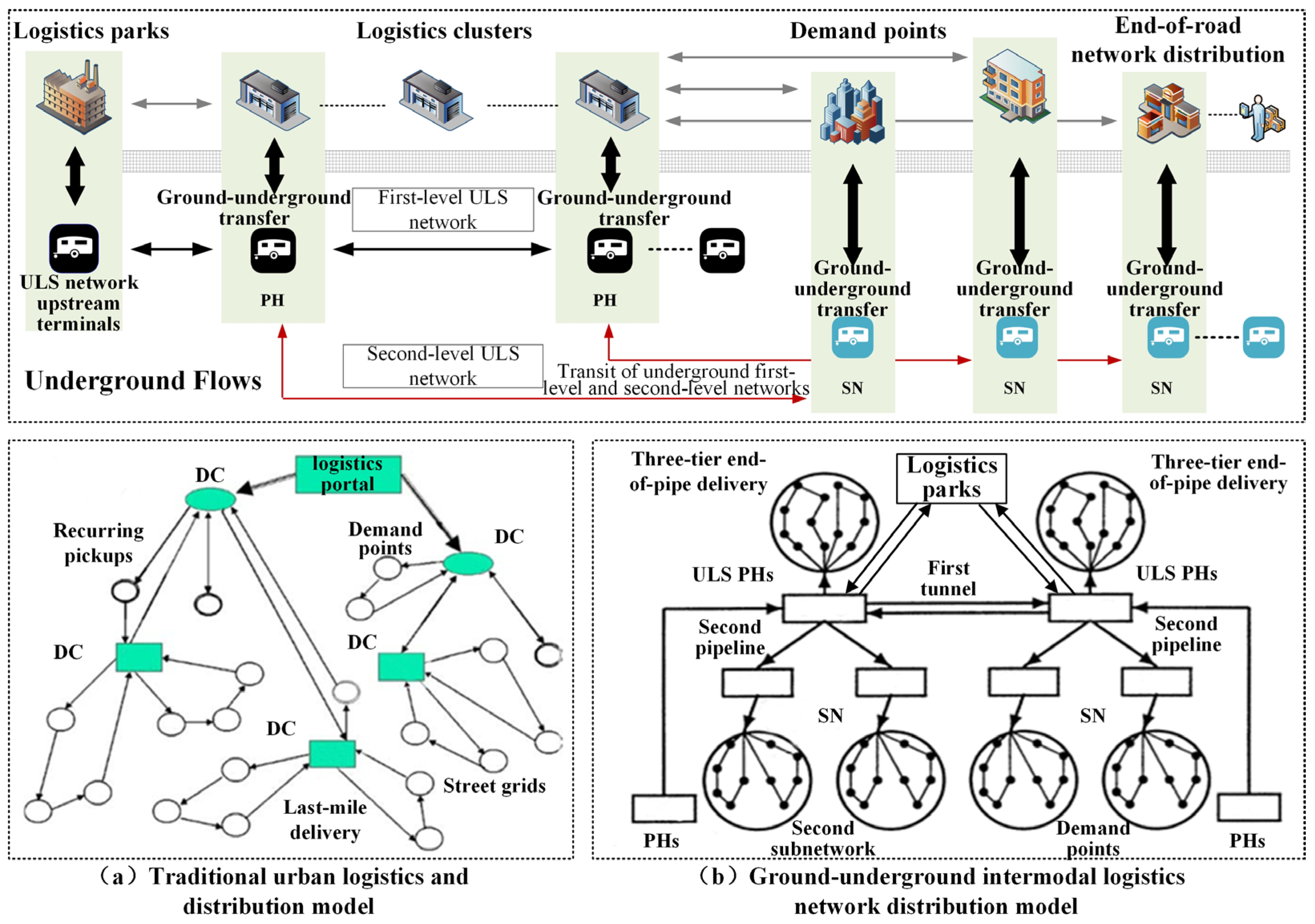
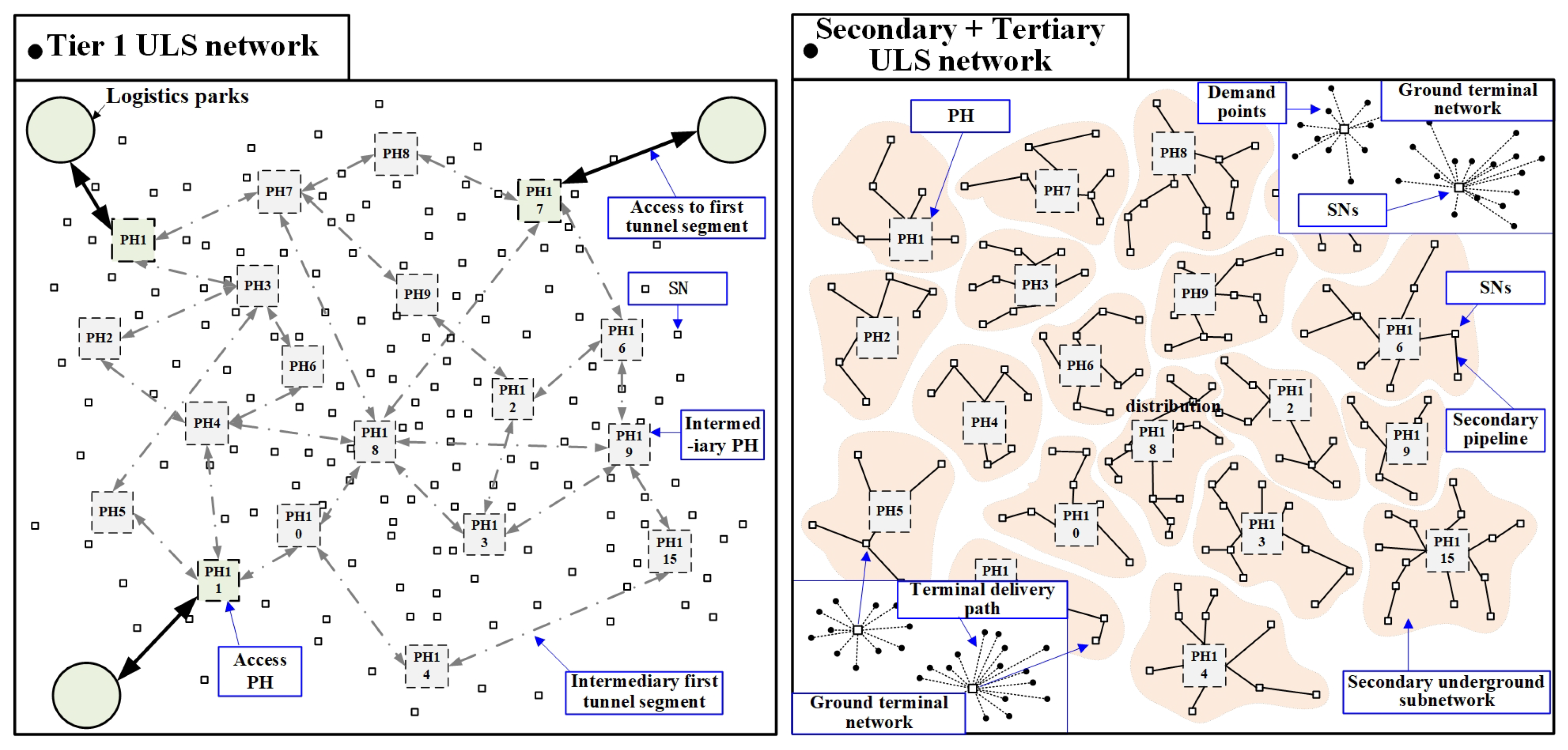
2.2.1. Composition of the Three-Tier Hub-and-Spoke ULS Network

ULS networks are structured into different hierarchical levels based on city size. In small- and medium-sized cities with relatively low logistics demand and only a limited number of logistics gateway facilities, a single-layer underground freight transportation network is generally considered sufficient [2,11]. In this configuration, goods are transported from industrial parks through tunnels to ULS nodes distributed across the city, followed by last-mile delivery via secondary surface road networks.

However, in mega-cities such as Beijing and Shanghai, a single-layer underground network would result in an overly dense tunnel distribution, which is unfavorable for underground vehicle operations and automated transportation activities. Moreover, the substantial logistics demand in large and mega-cities necessitates secondary freight distribution underground to reduce the operational burden on individual nodes.

To address these design challenges, this study proposes a hub-and-spoke ULS network topology composed of four node levels and three network layers. This topology effectively aligns with the organizational structure of large urban logistics systems, enabling the relocation of most urban distribution activities from surface roads to underground networks while ensuring seamless integration with surface logistics systems. By doing so, it aims to alleviate urban traffic congestion, mitigate challenges associated with freight vehicle access to city centers, and reduce environmental pollution. The definitions and operational mechanisms of various node levels and corridors within the ULS network are illustrated in Figure 1 and Figure 2. It is important to note that this prototype represents the final configuration of a fully developed ULS network a mega-city, whereas in small- and medium-sized cities, the secondary underground network layer may be omitted.

(1) Logistics parks.

According to China’s urban planning framework, major urban logistics hubs are typically located on the periphery of cities. These include multiple logistics parks, large freight yards/warehouses, and rail, seaport, and airport container terminals, as well as industrial zones. Some hub cities are equipped with varying numbers of provincial, municipal, or national-level logistics gateways, such as Qingdao’s “Belt and Road” logistics development axis and the Shanghai Port Free Trade Zone. In this study, these facilities are collectively referred to as “logistics parks”. Logistics parks serve as upstream terminals in the urban logistics system, connecting the city’s expressways and external trunk roads. They are typically located 50–100 km from the city center. Under conventional logistics models, freight from long-haul logistics routes is transported to front-end distribution centers (DCs) using container trucks and box trucks. These DCs, often positioned at cities’ boundaries (e.g., the Fifth Ring Road in the Beijing case study), receive goods from surface freight vehicles and further distribute them to urban distribution centers.

In ULSs, logistics parks function as the highest-tier nodes within the network. Due to traffic restrictions, most freight from these parks is only permitted to enter the city during night-time hours. To integrate with the ULS, logistics parks will be equipped with underground railway interfaces, while nearby rail depots will be scheduled to dispatch empty vehicles to these parks. At the logistics parks, cargo—having already been sorted, encoded, and packaged according to standardized procedures—will be loaded into designated forward O-D freight units. Subsequently, fully loaded locomotives will depart from the logistics parks and travel through the primary tunnel (PT), which connects the parks to the Primary Hub (PH)—the entry hub of the ULS. To minimize the length of PT segments and reduce costs, PH nodes are typically located near city boundaries, making front-end DCs a viable option for ULS hub placement.

(2) Urban logistics clusters/ULS hub nodes.

To distribute freight flow more effectively, this study proposes the establishment of additional ULS hub nodes within metropolitan areas. Hub nodes that are not directly connected to industrial parks are defined as intermediary hub nodes (or intermediary PHs). These intermediary PHs and access PHs are interconnected via first-tier intermediary tunnel segments (referred to as intermediary PTs), which are designed to match the specifications of access PTs, ensuring the seamless operation of rail-guided freight vehicles between hub nodes. Considering the alignment between underground freight movement and conventional urban distribution flow, the locations of intermediary PTs are generally selected from two types of sites. First, existing urban distribution centers can be repurposed by modifying their underground spaces to accommodate freight platforms for loading and unloading freight units. These modified DCs should also be equipped with a suite of automated handling facilities, including horizontal and vertical transport systems and integrated logistics processing equipment for on-site operations such as sorting, temporary storage, parcel disassembly, and quality inspection. Second, given the limited number of urban DCs, new ULS hub nodes may be established in high-demand areas without dedicated distribution centers. These locations may include commercial districts, central business districts (CBDs), residential clusters, and high-density urban neighborhoods. As discussed in Section 2.2.1, intra-city distribution activities occur among urban logistics clusters, and the implementation of hub nodes and first-tier tunnels facilitates partial underground transportation for intra-city origin-destination (O-D) pairs.

(3) ULS spoke nodes/demand points.

The service coverage of a single hub node is defined as a first-tier region, within which the number of customer demand points can range from several dozen to several hundred, depending on the distribution of hub nodes. The forward O-D distribution process, which covers transportation from the hub node to the final customer destination, is accomplished through two primary methods.

Mode 1: After processing at the hub node, parcels are directly lifted to the aboveground DC, a process defined as tertiary surface transshipment. The final distribution follows conventional last-mile delivery methods, where couriers use logistics vehicles to transport packages to designated delivery points near the hub node, such as community centers, buildings, parcel lockers, and delivery stations.

Mode 2: For demand points within a first-tier region that are located farther from the hub node, this study considers expanding the underground spaces of selected buildings to establish ULS spoke nodes (SNs). These spoke nodes are connected to hub nodes via a hierarchical secondary tunnel network (ST). Each spoke node serves a defined number of demand points based on its capacity and coverage radius. The secondary tunnels accommodate small-diameter capsule rail vehicles for freight transportation. Once processing is completed at the hub node, parcels are loaded onto capsule vehicles (secondary underground transshipment), transported through the secondary tunnel network to spoke nodes, and then lifted to the surface for final distribution. This last step mirrors the process in Mode 1, referred to as last-mile delivery (LMD), ensuring parcels reach their designated demand points.

To simplify the description, this study defines the following three-tiered ULS network structure: (i) The primary underground transport network consists of logistics parks, access hub nodes, intermediary hub nodes, first-tier tunnel access segments, and intermediary first-tier tunnel segments. (ii) The secondary underground transport network is composed of access hub nodes, intermediary hub nodes, spoke nodes, and secondary tunnel segments. (iii) The tertiary surface terminal network comprises access hub nodes, intermediary hub nodes, spoke nodes, and the last-mile road network. Together, these three interconnected layers form a comprehensive urban ULS topology.

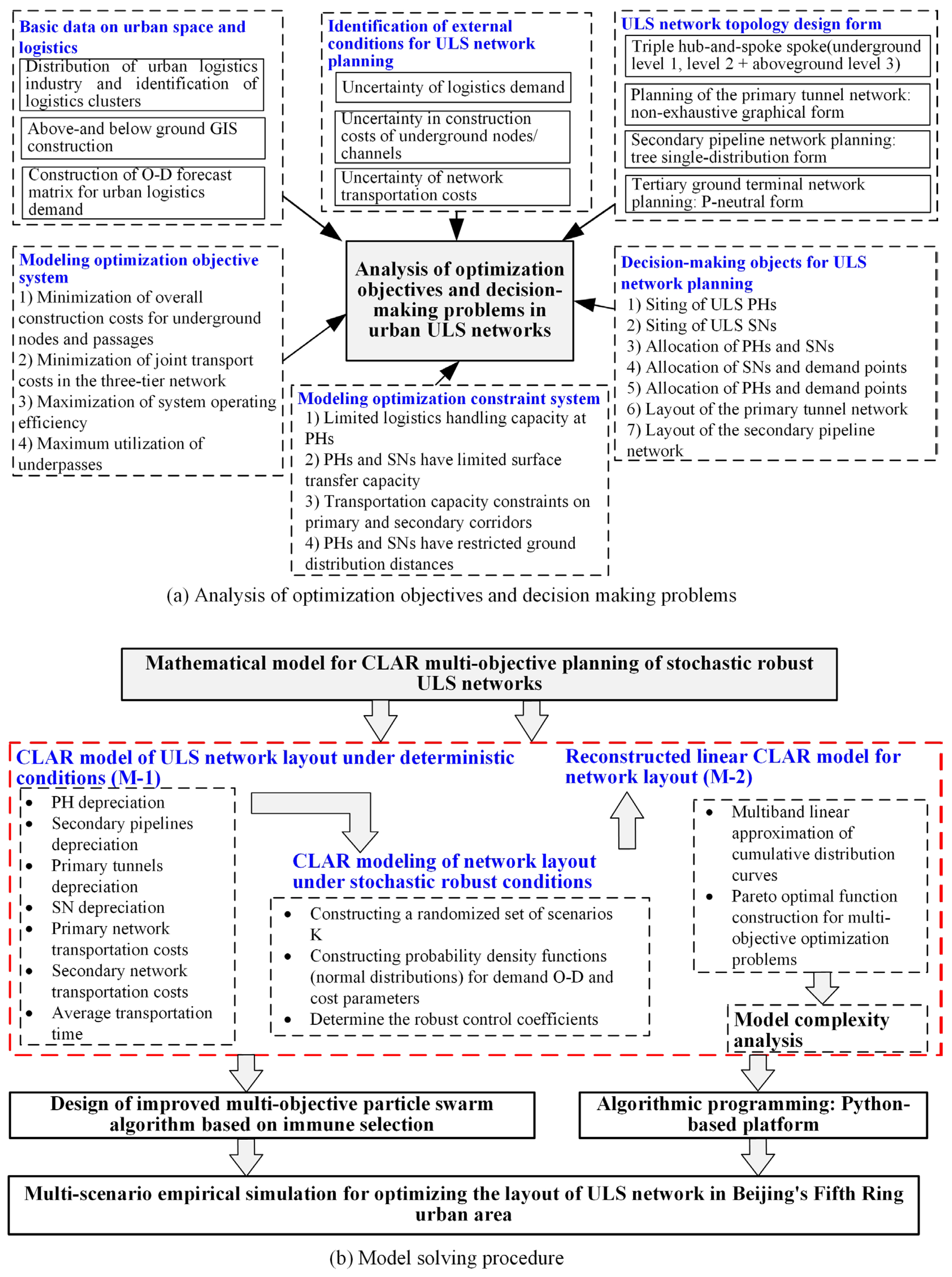
2.2.2. Multi-Objective Capacity Siting, Allocation, and Path Decision-Making

Based on the proposed topological structure, the overall objective of urban ULS network layout planning is to achieve an optimized configuration while minimizing both underground infrastructure construction costs and three-tier network transportation costs. This optimization involves the following eight key decision variables:

Decision 1: Determine the locations of access hub nodes and their corresponding relationships with urban logistics parks (Hub PH Location Selection).

Decision 2: Select an appropriate number and locations of logistics cluster points to establish intermediary hub nodes (Intermediary PH Location Selection).

Decision 3: Identify suitable demand points within each first-tier region to be developed as spoke nodes (SN Location Selection).

Decision 4: Establish the allocation relationships between spoke nodes and hub nodes within the secondary network (PH-SN Assignment).

Decision 5: Determine the allocation relationships between demand points and spoke nodes within the tertiary network (SN–Demand Point Assignment).

Decision 6: Define the allocation relationships between demand points and hub nodes within the tertiary network (PH–Demand Point Assignment).

Decision 7: Design the tunnel layout for the primary network and determine the transport routes for both forward O-D and intra-city O-D shipments within this network (Primary Network Path Planning).

Decision 8: Plan the pipeline layout for the secondary network and optimize the transport routes for forward O-D shipments within this network (Secondary Network Path Planning).

In ULS networks, first-tier tunnels are constructed within the city’s deep underground space, whereas secondary pipelines, requiring frequent access to the surface, are more suitable for shallow-buried construction. However, in high-density urban areas, shallow underground space is a scarce resource, limiting the available space for ULS node and corridor development. As a result, ULS nodes and tunnels face significant spatial constraints. For instance, large-scale automated storage systems cannot be accommodated within underground nodes, necessitating the rapid processing and dispatching of inbound shipments from the first-tier network to prevent congestion and ensure subsequent smooth operations. This characteristic resembles the operational model of a compact, pass-through distribution center.

This study considers five primary capacity constraints: (1) the secondary transshipment capacity of hub nodes, (2) the tertiary transshipment capacity of hub nodes, (3) the tertiary transshipment capacity of spoke nodes, (4) the transportation capacity of first-tier tunnels, (5) the transportation capacity of secondary pipelines. In addition to facility capacity constraints, this study also imposes a maximum allowable last-mile delivery distance within the tertiary network, ensuring that all deliveries remain within a predefined threshold. This restriction minimizes reliance on couriers and facilitates a door-to-door underground delivery system.

Existing ULS network layout studies typically focus on minimizing construction and transportation costs [1]. In contrast, this study simultaneously optimizes three objectives: minimizing network costs, maximizing operational efficiency, and maximizing underground corridor load utilization. This integrated approach aims to develop a more comprehensive multi-objective mathematical model for ULS network planning.

From a modeling perspective, existing ULS network studies primarily focus on deterministic decision optimization, while stochastic optimization and robust optimization theories addressing ULS demand O-D variations and system cost parameters remain underdeveloped. The model proposed in this chapter incorporates multidimensional uncertainties in network layout decision-making.

In summary, the modeling and optimization process of the three-tier hub-and-spoke ULS network belongs to a class of stochastic robust multi-objective Capacity–Location–Allocation–Routing (CLAR) problems. The overall modeling and optimization framework is illustrated in Figure 3a,b.

2.2.3. Parameters and Assumption

The modeling parameters for this paper are detailed in

Table 1. Model Parameters.

Symbol Definition	Variable Description
Constants and continuous variables
$d_{sj}$	Forecasted freight O-D volume between any park and demand point
${\delta }_{i{i}^{\prime }}$	Forecasted freight O-D volume between any logistics hubs
${\gamma }_{PH}$, ${\gamma }_{SN}$	Forecasted fixed construction costs for ULS hub nodes (PHs) and spoke nodes (SNs)
${\upsilon }_{PT}$	Forecasted unit fixed construction costs for first-tier tunnel segments
${\upsilon }_{ST}$	Forecasted unit fixed construction costs for secondary pipeline segments
$\mathsf{\alpha }$	Forecasted unit O-D transportation costs for first-tier ULS network
$\mathsf{\beta }$	Forecasted unit O-D transportation costs for secondary ULS network
c	Unit transportation costs for road-based freight O-D
[cap1], [cap2]	Maximum secondary underground transshipment capacity and tertiary surface transshipment capacity for PHs
[cap3]	Maximum tertiary surface transshipment capacity for SNs
[cap4], [cap5]	Maximum bidirectional freight transportation capacity for first-tier tunnels and secondary pipelines
${\epsilon }_{PT}$, ${\epsilon }_{ST}$	Maximum allowable unsaturation rate for first-tier tunnels and secondary pipelines
${\eta }_{PT}$, ${\eta }_{ST}$	Penalty costs resulting from saturation in first-tier tunnels and secondary pipelines
$EU\left(·\right)$	Euclidean distance function reflecting links g, h, p, q
ro	Maximum surface transportation distance for tertiary network
${\tau }_{PT}$, ${\tau }_{ST}$, ${\tau }_{LMD}$	Travel speeds for underground and surface transportation systems in first-tier, secondary, and tertiary networks
${\omega }_{PH}$, ${\omega }_{SN}$	Forecasted logistics handling time for O-D at hub and spoke nodes
$\theta$	Depreciation coefficient for ULS network infrastructure
${\mathsf{\Omega }}_k$	Probability of scenario k occurrence
Variables
$A_i^k$	In random scenario k, if logistics hub i is constructed as PH, then 1; otherwise, 0.
$B_j^k$	In random scenario k, if demand point j is constructed as SN, then 1; otherwise, 0.
${\xi }_g^k$	In random scenario k, if link g is constructed as access PT, then 1; otherwise, 0.
${\zeta }_h^k$	In random scenario k, if link h is constructed as intermediary PT, then 1; otherwise, 0.
${\phi }_p^k$	In random scenario k, if link p is constructed as ST, then 1; otherwise, 0;
${\rho }_q^k$	In random scenario k, if link q is constructed as ST, then 1; otherwise, 0;
$X_{sij}^k$	In random scenario k, if $d_{sj}$ undergoes secondary underground transshipment at PH i, then 1; otherwise, 0;
$Y_{sj{j}^{\prime }}^k$	In random scenario k, if $d_{sj}$ undergoes tertiary surface transshipment at SN j, then 1; otherwise, 0;
$Z_{sij}^k$	In random scenario k, if $d_{sj}$ undergoes tertiary surface transshipment at PH i, then 1; otherwise, 0;
$U_{sjg}^k$	In random scenario k, if $d_{sj}$ passes through access PT link g, then 1; otherwise, 0;
$V_{sjh}^k$	In random scenario k, if $d_{sj}$ passes through intermediary PT link h, then 1; otherwise, 0;
$W_{i{i}^{\prime }h}^k$	In random scenario k, if ${\delta }_{i{i}^{\prime }}$ passes through intermediary PT link h, then 1; otherwise, 0;
$R_{sjp}^k$	In random scenario k, if $d_{sj}$ passes through ST link p, then 1; otherwise, 0;
$T_{sjq}^k$	In random scenario k, if $d_{sj}$ passes through ST link q, then 1; otherwise, 0;
$M_{sjq}^k$	In random scenario k, if $d_{sj}$ passes through LMD link q, then 1; otherwise, 0;
${\varsigma }_{sjp}^k$	In random scenario k, if $d_{sj}$ passes through LMD link p, then 1; otherwise, 0;

.

The stochastic characteristics of demand O-D, costs, and processing time in the ULS network planning problem are characterized through the following transformation methods. As shown in

Table 2. Representation of Stochastic Parameters.

Variables	Normally Distributed Mean and Variance	Cumulative Distribution Function	Upper	Lower	Number of Functions
$d_{sj}$	${\stackrel{⌢}{d}}_{sj}^k\sim N_{d_{sj}}^k\left(\mu , {\sigma }^2\right)$	$F_{d_{sj}}^k\left(x\right)$	$d_{sj}^{k\left(+\right)}$	$d_{sj}^{k\left(-\right)}$	$3790\times ‖K‖$
${\delta }_{i{i}^{\prime }}$	${\stackrel{⌢}{\delta }}_{i{i}^{\prime }}^k\sim N_{{\delta }_{i{i}^{\prime }}}^k\left(\mu , {\sigma }^2\right)$	$F_{{\delta }_{i{i}^{\prime }}}^k\left(x\right)$	${\delta }_{i{i}^{\prime }}^{k\left(+\right)}$	${\delta }_{i{i}^{\prime }}^{k\left(-\right)}$	$5776\times ‖K‖$
${\gamma }_{PH}$	${\stackrel{⌢}{\gamma }}_{PH}^k\sim N_{{\gamma }_{PH}}^k\left(\mu , {\sigma }^2\right)$	$F_{{\gamma }_{PH}}^k\left(x\right)$	${\gamma }_{PH}^{k\left(+\right)}$	${\gamma }_{PH}^{k\left(-\right)}$	$‖K‖$
${\gamma }_{SN}$	${\stackrel{⌢}{\gamma }}_{SN}^k\sim N_{{\gamma }_{SN}}^k\left(\mu , {\sigma }^2\right)$	$F_{{\gamma }_{SN}}^k\left(x\right)$	${\gamma }_{SN}^{k\left(+\right)}$	${\gamma }_{SN}^{k\left(-\right)}$	$‖K‖$
${\upsilon }_{PT}$	${\stackrel{⌢}{\upsilon }}_{PT}^k\sim N_{{\upsilon }_{PT}}^k\left(\mu , {\sigma }^2\right)$	$F_{{\upsilon }_{PT}}^k\left(x\right)$	${\upsilon }_{PT}^{k\left(+\right)}$	${\upsilon }_{PT}^{k\left(-\right)}$	$‖K‖$
${\upsilon }_{ST}$	${\stackrel{⌢}{\upsilon }}_{ST}^k\sim N_{{\upsilon }_{ST}}^k\left(\mu , {\sigma }^2\right)$	$F_{{\upsilon }_{ST}}^k\left(x\right)$	${\upsilon }_{ST}^{k\left(+\right)}$	${\upsilon }_{ST}^{k\left(-\right)}$	$‖K‖$
$\mathsf{\alpha }$	${\stackrel{⌢}{\mathsf{\alpha }}}_k\sim N_{\mathsf{\alpha }}^k\left(\mu , {\sigma }^2\right)$	$F_{\mathsf{\alpha }}^k\left(x\right)$	${\mathsf{\alpha }}_k^{+}$	${\mathsf{\alpha }}_k^{-}$	$‖K‖$
$\mathsf{\beta }$	${\stackrel{⌢}{\mathsf{\beta }}}_k\sim N_{\mathsf{\beta }}^k\left(\mu , {\sigma }^2\right)$	$F_{\mathsf{\beta }}^k\left(x\right)$	${\mathsf{\beta }}_k^{+}$	${\mathsf{\beta }}_k^{-}$	$‖K‖$
${\omega }_{PH}$	${\stackrel{⌢}{\omega }}_{PH}^k\sim N_{{\omega }_{PH}}^k\left(\mu , {\sigma }^2\right)$	$F_{{\omega }_{PH}}^k\left(x\right)$	${\omega }_{PH}^{k\left(+\right)}$	${\omega }_{PH}^{k\left(-\right)}$	$‖K‖$
${\omega }_{SN}$	${\stackrel{⌢}{\omega }}_{SN}^k\sim N_{{\omega }_{SN}}^k\left(\mu , {\sigma }^2\right)$	$F_{{\omega }_{SN}}^k\left(x\right)$	${\omega }_{SN}^{k\left(+\right)}$	${\omega }_{SN}^{k\left(-\right)}$	$‖K‖$

, the predicted values of four key parameters—(i) the fixed costs of various ULS nodes and corridors $\left\{{\gamma }_{PH}, {\gamma }_{SN}, {\upsilon }_{PT}, {\upsilon }_{ST}\right\}$, (ii) the predicted underground freight transportation costs $\left\{\mathsf{\alpha }, \mathsf{\beta }\right\}$, (iii) the predicted processing times at ULS nodes $\left\{{\omega }_{PH}, {\omega }_{SN}\right\}$, (iv) the predicted freight demand O-D volumes $\left\{d_{sj}, {\delta }_{i{i}^{\prime }}\right\}$—are assumed to follow a normal distribution within their respective ranges. Taking ${\gamma }_{PH}$ as an example, the actual value ${\stackrel{⌢}{\gamma }}_{PH}^k$ of ${\gamma }_{PH}$ in random scenario k follows a probability density function $f_{{\gamma }_{PH}}^k\left(x\right)$ and conforms to ${\stackrel{⌢}{\gamma }}_{PH}^k\sim N_{{\gamma }_{PH}}^k\left(\mu , {\sigma }^2\right)$. The lower bound of the 95% confidence interval of the probability density function is denoted as ${\gamma }_{PH}^{k\left(-\right)}$, representing the minimum possible construction cost of ULS hub node i. Similarly, the upper bound of the 95% confidence interval of the distribution function is denoted as ${\gamma }_{PH}^{k\left(+\right)}$, representing the maximum possible construction cost. Finally, by integrating $f_{{\gamma }_{PH}}^k\left(x\right)$, the cumulative distribution function $F_{{\gamma }_{PH}}^k\left(x\right)$ of ULS hub node construction cost is obtained. According to Equation (1), the value of the cumulative distribution function represents the sum of probabilities for all discrete values of ${\stackrel{⌢}{\gamma }}_{PH}^k$ that are less than or equal to x. For example, it quantifies the cumulative probability that the actual construction cost of a node $F_{{\gamma }_{PH}}^k\left({\gamma }_{PH}\right)$ is lower than its predicted value. Random scenario k is generated by combining different probability density functions for all 10 stochastic variables. In the case study of Beijing, each individual random scenario requires the construction of 9574 probability density functions.

$$\left\{\begin{array}{l}{F}_{{\gamma }_i}^k\left(x\right)={\displaystyle {\int }_{-\infty }^x{f}_{{\gamma }_i}^k\left(t\right) }\mathrm{d}t\\ F_{{\gamma }_i}^k\left({\gamma }_i\right)=\mathrm{P}\left(x\le {\gamma }_i\right)\end{array}\right., \mathrm{for}\forall x\in \left[{\gamma }_{ik}^{-}, {\gamma }_{ik}^{+}\right], i\in N, k\in K$$

(1)

The following fundamental assumptions are made regarding urban ULS network layout optimization in this study:

Assumption 1. 

Each segment of the first-tier tunnels and second-tier pipelines in the ULS network is modeled as a direct point-to-point connection. The impact of geological conditions and construction constraints on underground nodes and corridors is not considered.

Assumption 2. 

The first-tier ULS network is structured as an incomplete graph, where each hub node can be connected to one or more other hub nodes via underground tunnels. The second-tier ULS network follows a single-assignment tree-like pipeline structure, where each local secondary network has a unique “root” node (hub) and multiple “branch” nodes (spokes). The third-tier ULS network adopts a P-median single-assignment surface routing approach, meaning that each demand point is assigned to a single hub or spoke node and is directly connected to its assigned upper-tier node.

Assumption 3. 

Urban freight O-D transportation between logistics hubs utilizes only the capacity of first-tier tunnels without consuming transshipment capacity at hub nodes. Additionally, freight flows passing through a hub node via first-tier tunnels do not occupy any processing capacity at that hub. The transportation capacity of access PTs is considered unlimited.

Assumption 4. 

The impact of dynamic scheduling processes during system operation on facility location planning is disregarded. This includes factors such as passenger-freight time windows, inbound and outbound logistics rules, and transshipment policies.

Assumption 5. 

The forecasted demand volumes for forward/reverse logistics O-D and urban freight distribution O-D at demand points are assumed to be known. The demand O-D at each demand point is derived from the total forecasted logistics volume of Beijing, as outlined in Section 3.3.3, and allocated based on land parcel population density.

Assumption 6: 

If a demand point is designated as a service node within the ULS network, all of its freight orders relative to logistics parks are assumed to be transported exclusively through the ULS network.

Assumption 7: 

Not all demand points are required to be serviced by the ULS network. However, the ULS should maximize its capacity to accommodate as many demand points as possible, thereby expanding system coverage.

3. Model Development

3.1. Modeling Objectives

(1) Minimization of network construction costs.

The total construction cost of a ULS network consists of four components: hub node construction cost, spoke node construction cost, first-tier tunnel construction cost, and second-tier pipeline construction cost. These costs are annualized over a predefined depreciation period and further distributed on a daily basis. Under deterministic conditions, the minimization sub-objective function $f_{\mathrm{determ}}^{\left(1\right)}$ is formulated as shown in Equation (2). For the four categories of uncertain parameters ${\stackrel{⌢}{\gamma }}_{PH}^k$, ${\stackrel{⌢}{\gamma }}_{SN}^k$, ${\stackrel{⌢}{\upsilon }}_{ST}^k$, and ${\stackrel{⌢}{\upsilon }}_{PT}^k$ involved in the equation, their approximate values under stochastic scenarios are derived using the sum of the lower bound of the probability distribution function and the integral of the cumulative distribution function within a confidence interval, based on mathematical statistics principles. Furthermore, following the approach proposed by [15], the weighted objective function $f_{\mathrm{random}}^{\left(1\right)\ast }$ under stochastic conditions is expressed in Equation (3), where it is computed as the summation of the product of the probability of each stochastic scenario and the approximate objective function value derived under that scenario.

When Equation (3) neither sums over the scenario set k nor considers the scenario probability ${\mathsf{\Omega }}_k$, the resulting function represents the stochastic objective value for each scenario, denoted as $f_{\mathrm{random}}^{\left(1\right)}\left(k_1\right)$, $f_{\mathrm{random}}^{\left(1\right)}\left(k_2\right)$, … $f_{\mathrm{random}}^{\left(1\right)}\left(k_n\right)$. Subsequently, the differences between the stochastic objective function values under each scenario and the weighted objective function value under stochastic conditions are squared and summed. A robustness coefficient is introduced to reflect the decision-maker’s preference. A higher value of $\mathsf{\Gamma }$ indicates a stronger emphasis on system robustness, meaning that the decision-maker adopts a more conservative approach toward the expected risks associated with the current decision, characteristic of risk-averse behavior. Conversely, a lower R value implies a more risk-tolerant attitude. Finally, the stochastic robust value for the minimization of ULS network construction costs is computed according to Equation (4)

$$\begin{array}{l}\min f_{\mathrm{determ}}^{\left(1\right)}={\theta }^{-1}\cdot {\gamma }_{PH}\cdot {\displaystyle \sum _{i\in N}{A}_i}+{\theta }^{-1}\cdot {\upsilon }_{ST}\cdot {\displaystyle \sum _{p\in P}{\displaystyle \sum _{q\in Q}\left(E{u}_p\cdot {\phi }_p+E{u}_q\cdot {\rho }_q\right)}}\\ +{\theta }^{-1}\cdot {\upsilon }_{PT}\cdot {\displaystyle \sum _{g\in L}{\displaystyle \sum _{h\in H}\left(E{u}_g\cdot {\xi }_g+E{u}_h\cdot {\zeta }_h\right)}}+{\theta }^{-1}\cdot {\gamma }_{SN}\cdot {\displaystyle \sum _{j\in J}{B}_j}\end{array}$$

(2)

$$\begin{array}{l}\min f_{\mathrm{random}}^{\left(1\right)\ast }={\theta }^{-1}\cdot {\displaystyle \sum _{k\in K}{\mathsf{\Omega }}_k{\displaystyle \sum _{i\in N}{A}_i^k\cdot \left[{\gamma }_{PH}^{k\left(-\right)}+{\displaystyle {\int }_{{\gamma }_{PH}^{k\left(-\right)}}^{{\gamma }_{PH}^{k\left(+\right)}}{F}_{{\gamma }_i}^k\left(x\right)\mathrm{d}x}\right]}}\\ +{\theta }^{-1}\cdot {\displaystyle \sum _{k\in K}{\mathsf{\Omega }}_k{\displaystyle \sum _{p\in P}{\displaystyle \sum _{q\in Q}\left({\phi }_p^k\cdot E{u}_p+{\rho }_q^k\cdot E{u}_p\right)\cdot \left[{\upsilon }_{ST}^{k\left(-\right)}+{\displaystyle {\int }_{{\upsilon }_{ST}^{k\left(-\right)}}^{{\upsilon }_{ST}^{k\left(+\right)}}{F}_{{\upsilon }_{ST}}^k\left(x\right)\mathrm{d}x}\right]}}}\\ +{\theta }^{-1}\cdot {\displaystyle \sum _{k\in K}{\mathsf{\Omega }}_k{\displaystyle \sum _{g\in L}{\displaystyle \sum _{h\in H}\left({\xi }_g^k\cdot E{u}_g+{\zeta }_h^k\cdot E{u}_h\right)\cdot \left[{\upsilon }_{PT}^{k\left(-\right)}+{\displaystyle {\int }_{{\upsilon }_{PT}^{k\left(-\right)}}^{{\upsilon }_{PT}^{k\left(+\right)}}{F}_{{\upsilon }_{PT}}^k\left(x\right)\mathrm{d}x}\right]}}}\\ +{\theta }^{-1}\cdot {\displaystyle \sum _{k\in K}{\mathsf{\Omega }}_k{\displaystyle \sum _{j\in J}{B}_j^k\cdot \left[{\gamma }_{SN}^{k\left(-\right)}+{\displaystyle {\int }_{{\gamma }_{SN}^{k\left(-\right)}}^{{\gamma }_{SN}^{k\left(+\right)}}{F}_{{\gamma }_i}^k\left(x\right)\mathrm{d}x}\right]}}\end{array}$$

(3)

$$\min f_{\mathrm{robust}}^{\left(1\right)}=f_{\mathrm{random}}^{\left(1\right)\ast }-{\mathsf{\Gamma }}^{\left(1\right)}\cdot {\mathsf{\Omega }}_k\cdot \left[\begin{array}{l}{\left(f_{\mathrm{random}}^{\left(1\right)}\left(k_1\right)-f_{\mathrm{random}}^{\left(1\right)\ast }\right)}^2+{\left(f_{\mathrm{random}}^{\left(1\right)}\left(k_2\right)-f_{\mathrm{random}}^{\left(1\right)\ast }\right)}^2\\ +\cdots +{\left(f_{\mathrm{random}}^{\left(1\right)}\left(k_n\right)-f_{\mathrm{random}}^{\left(1\right)\ast }\right)}^2\end{array}\right]$$

(4)

(2) Minimization of network operating costs.

The operational cost of the ULS network comprises four components: the underground transportation cost of forward O-D flows in primary tunnels, the primary tunnel transportation cost of intra-city O-D flows, the secondary pipeline transportation cost of forward O-D flows, and the surface transportation cost within the tertiary terminal road network. These costs involve four categories of uncertain parameters: ${\stackrel{⌢}{d}}_{sj}^k$, ${\stackrel{⌢}{\delta }}_{i{i}^{\prime }}^k$, ${\stackrel{⌢}{\alpha }}_k$, and ${\stackrel{⌢}{\beta }}_k$. Based on the transformation method described above, the minimized operational cost sub-objective functions of the ULS network under deterministic conditions, stochastic conditions, and stochastic robust conditions are denoted as $f_{\mathrm{determ}}^{\left(2\right)}$ (Equation (5)), $f_{\mathrm{random}}^{\left(2\right)\ast }$ (Equation (6)), and $f_{\mathrm{robust}}^{\left(2\right)}$ (Equation (7)), respectively.

$$\begin{array}{l}\min f_{\mathrm{determ}}^{\left(2\right)\ast }=c\cdot {\displaystyle \sum _{s\in S}{\displaystyle \sum _{j\in J}{d}_{sj}{\displaystyle \sum _{q\in Q}{\displaystyle \sum _{p\in P}\left(M_{sjq}\cdot E{U}_q+{\varsigma }_{sjp}\cdot E{U}_q\right)}}}}\\ +\mathsf{\alpha }\cdot {\displaystyle \sum _{i\in N}{\displaystyle \sum _{i^{\prime }\in N}{\delta }_{i{i}^{\prime }}{\displaystyle \sum _{h\in H}{W}_{i{i}^{\prime }h}\cdot E{U}_h}}}\\ +\mathsf{\alpha }\cdot {\displaystyle \sum _{s\in S}{\displaystyle \sum _{j\in J}{d}_{sj}{\displaystyle \sum _{g\in L}{\displaystyle \sum _{h\in H}\left(U_{sjg}\cdot E{U}_g+V_{sjh}\cdot E{U}_h\right)}}}}\\ +\mathsf{\beta }\cdot {\displaystyle \sum _{s\in S}{\displaystyle \sum _{j\in J}{d}_{sj}{\displaystyle \sum _{p\in P}{\displaystyle \sum _{q\in Q}\left(R_{sjp}\cdot E{U}_p+T_{sjq}\cdot E{U}_q\right)}}}}\end{array}$$

(5)

$$\begin{array}{l}\min f_{\mathrm{random}}^{\left(2\right)}=c\cdot {\displaystyle \sum _{s\in S}{\displaystyle \sum _{j\in J}{\displaystyle \sum _{k\in K}{\mathsf{\Omega }}_k\left[d_{sj}^{k\left(-\right)}+{\displaystyle {\int }_{d_{sj}^{k\left(-\right)}}^{d_{sj}^{k\left(+\right)}}{F}_{d_{sj}}^k\left(x\right)\mathrm{d}x}\right]}{\displaystyle \sum _{q\in Q}{\displaystyle \sum _{p\in P}\left(M_{sjq}^k\cdot E{U}_q+{\varsigma }_{sjp}^k\cdot E{U}_q\right)}}}}\\ +{\displaystyle \sum _{s\in S}{\displaystyle \sum _{j\in J}{\displaystyle \sum _{k\in K}{\mathsf{\Omega }}_k\left[{\mathsf{\alpha }}_k^{-}+{\displaystyle {\int }_{{\mathsf{\alpha }}_k^{-}}^{{\mathsf{\alpha }}_k^{+}}{F}_{\mathsf{\alpha }}^k\left(x\right)\mathrm{d}x}\right]\times \left[d_{sj}^{k\left(-\right)}+{\displaystyle {\int }_{d_{sj}^{k\left(-\right)}}^{d_{sj}^{k\left(+\right)}}{F}_{d_{sj}}^k\left(x\right)\mathrm{d}x}\right]}{\displaystyle \sum _{g\in L}{\displaystyle \sum _{h\in H}\left(U_{sjg}^k\cdot E{U}_g+V_{sjh}^k\cdot E{U}_h\right)}}}}\\ +{\displaystyle \sum _{s\in S}{\displaystyle \sum _{j\in J}{\displaystyle \sum _{k\in K}{\mathsf{\Omega }}_k\left[{\mathsf{\beta }}_k^{-}+{\displaystyle {\int }_{{\mathsf{\beta }}_k^{-}}^{{\mathsf{\beta }}_k^{+}}{F}_{\mathsf{\beta }}^k\left(x\right)\mathrm{d}x}\right]\times \left[d_{sj}^{k\left(-\right)}+{\displaystyle {\int }_{d_{sj}^{k\left(-\right)}}^{d_{sj}^{k\left(+\right)}}{F}_{d_{sj}}^k\left(x\right)\mathrm{d}x}\right]}{\displaystyle \sum _{p\in P}{\displaystyle \sum _{q\in Q}\left(R_{sjp}^k\cdot E{U}_p+T_{sjq}^k\cdot E{U}_q\right)}}}}\\ +{\displaystyle \sum _{i\in N}{\displaystyle \sum _{i^{\prime }\in N}{\displaystyle \sum _{k\in K}{\mathsf{\Omega }}_k\left[{\mathsf{\alpha }}_k^{-}+{\displaystyle {\int }_{{\mathsf{\alpha }}_k^{-}}^{{\mathsf{\alpha }}_k^{+}}{F}_{\mathsf{\alpha }}^k\left(x\right)\mathrm{d}x}\right]\times \left[{\delta }_{i{i}^{\prime }}^{k\left(-\right)}+{\displaystyle {\int }_{{\delta }_{i{i}^{\prime }}^{k\left(-\right)}}^{{\delta }_{i{i}^{\prime }}^{k\left(+\right)}}{F}_{{\delta }_{i{i}^{\prime }}}^k\left(x\right)\mathrm{d}x}\right]}{\displaystyle \sum _{h\in H}{W}_{i{i}^{\prime }h}^k\cdot E{U}_h}}}\end{array}$$

(6)

$$\min f_{\mathrm{robust}}^{\left(2\right)}=f_{\mathrm{random}}^{\left(2\right)\ast }-{\mathsf{\Gamma }}^{\left(2\right)}\cdot {\mathsf{\Omega }}_k\cdot \left[\begin{array}{l}{\left(f_{\mathrm{random}}^{\left(2\right)}\left(k_1\right)-f_{\mathrm{random}}^{\left(2\right)\ast }\right)}^2+{\left(f_{\mathrm{random}}^{\left(2\right)}\left(k_2\right)-f_{\mathrm{random}}^{\left(2\right)\ast }\right)}^2\\ +\cdots +{\left(f_{\mathrm{random}}^{\left(2\right)}\left(k_n\right)-f_{\mathrm{random}}^{\left(2\right)\ast }\right)}^2\end{array}\right]$$

(7)

(3) Maximization of system operational efficiency.

The operational efficiency of a ULS is evaluated based on the average time required to complete the transportation and logistics processes for each forward freight order within the ULS network. For a single forward O-D, the total transit time within the network consists of up to five components: (i) Underground travel time within the first-tier tunnel network (from the logistics park to the destination hub node). (ii) Logistics processing time at the hub node. (iii) Underground travel time within the second-tier pipeline network (from the hub node to the destination spoke node). (iv) Logistics processing time at the spoke node. (v) Surface travel time within the third-tier terminal road network (from the spoke node to the customer location). Based on the above description, the operational efficiency maximization sub-objective functions for a three-tier ULS network under deterministic, stochastic, and stochastic robust conditions, which corresponds to the minimization of the average order transit time, are denoted as $f_{\mathrm{determ}}^{\left(3\right)}$ (Equation (8)), $f_{\mathrm{random}}^{\left(3\right)\ast }$ (Equation (9)), and $f_{\mathrm{robust}}^{\left(3\right)}$ (Equation (10)), respectively. In these equations, def represents the node processing time scaling factor, with a value of 500.

$$\begin{array}{l}\min f_{\mathrm{determ}}^{\left(3\right)}={\displaystyle \frac{{\displaystyle \sum _{s\in S}{\displaystyle \sum _{j\in J}{\displaystyle \sum _{g\in L}{\displaystyle \sum _{h\in H}\left(U_{sjg}\cdot E{U}_g+V_{sjh}\cdot E{U}_h\right)}}}}}{{\tau }_{PT}\cdot {\displaystyle \sum _{s\in S}{\displaystyle \sum _{j\in J}{\displaystyle \sum _{g\in L}{U}_{sjg}}}}}}+{\displaystyle \frac{{\omega }_{PH}}{def}}+{\displaystyle \frac{{\omega }_{SN}\cdot {\displaystyle \sum _{s\in S}{\displaystyle \sum _{i\in N}{\displaystyle \sum _{j\in J}{X}_{sij}}}}}{def\cdot {\displaystyle \sum _{s\in S}{\displaystyle \sum _{j\in J}{\displaystyle \sum _{g\in L}{U}_{sjg}}}}}}\\ +{\displaystyle \frac{{\displaystyle \sum _{s\in S}{\displaystyle \sum _{j\in J}{\displaystyle \sum _{p\in P}{\displaystyle \sum _{q\in Q}\left(R_{sjp}\cdot E{U}_p+T_{sjq}\cdot E{U}_q\right)}}}}}{{\tau }_{ST}\cdot {\displaystyle \sum _{s\in S}{\displaystyle \sum _{j\in J}{\displaystyle \sum _{g\in L}{U}_{sjg}}}}}}+{\displaystyle \frac{{\displaystyle \sum _{s\in S}{\displaystyle \sum _{j\in J}{\displaystyle \sum _{q\in Q}{\displaystyle \sum _{p\in P}\left(M_{sjq}\cdot E{U}_q+{\varsigma }_{sjp}\cdot E{U}_q\right)}}}}}{{\tau }_{LMD}\cdot {\displaystyle \sum _{s\in S}{\displaystyle \sum _{j\in J}{\displaystyle \sum _{g\in L}{U}_{sjg}}}}}}\end{array}$$

(8)

$$\begin{array}{l}\min f_{\mathrm{random}}^{\left(3\right)*}={\displaystyle \frac{{\displaystyle \sum _{k\in K}{\mathsf{\Omega }}_k{\displaystyle \sum _{s\in S}{\displaystyle \sum _{j\in J}{\displaystyle \sum _{g\in L}{\displaystyle \sum _{h\in H}\left(U_{sjg}^k\cdot E{U}_g+V_{sjh}^k\cdot E{U}_h\right)}}}}}}{{\tau }_{PT}\cdot {\displaystyle \sum _{k\in K}{\mathsf{\Omega }}_k{\displaystyle \sum _{s\in S}{\displaystyle \sum _{j\in J}{\displaystyle \sum _{g\in L}{U}_{sjg}^k}}}}}}+{\displaystyle \sum _{k\in K}{\mathsf{\Omega }}_k\left[\frac{{\omega }_{PH}^{k\left(-\right)}}{def}+{\displaystyle {\int }_{{\omega }_{PH}^{k\left(-\right)}}^{{\omega }_{PH}^{k\left(+\right)}}{F}_{{\omega }_{PH}}^k\left(x\right)\mathrm{d}x}\right]}\\ +{\displaystyle \frac{{\displaystyle \sum _{k\in K}{\mathsf{\Omega }}_k{\displaystyle \sum _{s\in S}{\displaystyle \sum _{j\in J}{\displaystyle \sum _{p\in P}{\displaystyle \sum _{q\in Q}\left(R_{sjp}^k\cdot E{U}_p+T_{sjq}^k\cdot E{U}_q\right)}}}}}}{{\tau }_{ST}\cdot {\displaystyle \sum _{k\in K}{\mathsf{\Omega }}_k{\displaystyle \sum _{s\in S}{\displaystyle \sum _{j\in J}{\displaystyle \sum _{g\in L}{U}_{sjg}^k}}}}}}+{\displaystyle \frac{{\displaystyle \sum _{k\in K}\left[\frac{{\omega }_{SN}^{k\left(-\right)}}{def}+{\displaystyle {\int }_{{\omega }_{SN}^{k\left(-\right)}}^{{\omega }_{SN}^{k\left(+\right)}}{F}_{{\omega }_{SN}}^k\left(x\right)\mathrm{d}x}\right]{\mathsf{\Omega }}_k{\displaystyle \sum _{s\in S}{\displaystyle \sum _{i\in N}{\displaystyle \sum _{j\in J}{X}_{sij}^k}}}}}{{\displaystyle \sum _{k\in K}{\mathsf{\Omega }}_k{\displaystyle \sum _{s\in S}{\displaystyle \sum _{j\in J}{\displaystyle \sum _{g\in L}{U}_{sjg}^k}}}}}}\\ +{\displaystyle \frac{{\displaystyle \sum _{k\in K}{\mathsf{\Omega }}_k{\displaystyle \sum _{s\in S}{\displaystyle \sum _{j\in J}{\displaystyle \sum _{q\in Q}{\displaystyle \sum _{p\in P}\left(M_{sjq}^k\cdot E{U}_q+{\varsigma }_{sjp}^k\cdot E{U}_q\right)}}}}}}{{\tau }_{LMD}\cdot {\displaystyle \sum _{k\in K}{\mathsf{\Omega }}_k{\displaystyle \sum _{s\in S}{\displaystyle \sum _{j\in J}{\displaystyle \sum _{g\in L}{U}_{sjg}^k}}}}}}\end{array}$$

(9)

$$\min f_{\mathrm{robust}}^{\left(3\right)}=f_{\mathrm{random}}^{\left(3\right)\ast }-{\mathsf{\Gamma }}^{\left(3\right)}\cdot {\mathsf{\Omega }}_k\cdot \left[\begin{array}{l}{\left(f_{\mathrm{random}}^{\left(3\right)}\left(k_1\right)-f_{\mathrm{random}}^{\left(3\right)\ast }\right)}^2+{\left(f_{\mathrm{random}}^{\left(3\right)}\left(k_2\right)-f_{\mathrm{random}}^{\left(3\right)\ast }\right)}^2\\ +\cdots +{\left(f_{\mathrm{random}}^{\left(3\right)}\left(k_n\right)-f_{\mathrm{random}}^{\left(3\right)\ast }\right)}^2\end{array}\right]$$

(10)

(4) Maximization of underground channel load.

The first-tier tunnel facilities and second-tier pipeline facilities in a ULS network should aim to maximize their load capacity, thereby reducing the total length of underground passages and consequently lowering both the construction and operational costs of the network. The load capacity of an underground passage is determined by dividing the daily transport volume of that passage by its capacity. When the load falls below the maximum allowable vacancy rate, a vacancy penalty cost is incurred based on the degree of unmet capacity. The objective of ULS network planning is to minimize the vacancy penalty costs for all planned passages. Using the transformation method outlined above, the maximization sub-objective functions for the channel load in a three-tier ULS network under deterministic, stochastic, and stochastic robust conditions are denoted as $f_{\mathrm{determ}}^{\left(4\right)}$ (Equation (11)), $f_{\mathrm{random}}^{\left(4\right)\ast }$ (Equation (12)), and E (Equation (13)), respectively.

$$\begin{array}{l}\min f_{\mathrm{determ}}^{\left(4\right)}={\displaystyle \sum _{h\in H}\max \left\{{\displaystyle \sum _{s\in S}{\displaystyle \sum _{j\in J}{d}_{sj}\cdot V_{sjh}}}+{\displaystyle \sum _{i\in N}{\displaystyle \sum _{i^{\prime }\in N}{\delta }_{i{i}^{\prime }}\cdot W_{i{i}^{\prime }h}}}-{\epsilon }_{PT}\cdot \left[ca{p}_4\right], 0\right\}\cdot {\eta }_{PT}}\\ +{\displaystyle \sum _{p\in P}\max \left\{{\displaystyle \sum _{s\in S}{\displaystyle \sum _{j\in J}{d}_{sj}\cdot R_{sjp}}}-{\epsilon }_{ST}\cdot \left[ca{p}_5\right], 0\right\}\cdot {\eta }_{ST}}\\ +{\displaystyle \sum _{q\in Q}\max \left\{{\displaystyle \sum _{s\in S}{\displaystyle \sum _{j\in J}{d}_{sj}\cdot T_{sjq}}}-{\epsilon }_{ST}\cdot \left[ca{p}_5\right], 0\right\}\cdot {\eta }_{ST}}\end{array}$$

(11)

$$\begin{array}{l}\min f_{\mathrm{random}}^{\left(4\right)}={\displaystyle \sum _{h\in H}\max \left\{\begin{array}{l}{\displaystyle \sum _{i\in N}{\displaystyle \sum _{i^{\prime }\in N}{\displaystyle \sum _{k\in K}{\mathsf{\Omega }}_k\left[{\delta }_{i{i}^{\prime }}^{k\left(-\right)}+{\displaystyle {\int }_{{\delta }_{i{i}^{\prime }}^{k\left(-\right)}}^{{\delta }_{i{i}^{\prime }}^{k\left(+\right)}}{F}_{{\delta }_{i{i}^{\prime }}}^k\left(x\right)\mathrm{d}x}\right]\cdot W_{i{i}^{\prime }h}^k}}}-{\epsilon }_{PT}\cdot \left[ca{p}_4\right]\\ +{\displaystyle \sum _{s\in S}{\displaystyle \sum _{j\in J}{\displaystyle \sum _{k\in K}{\mathsf{\Omega }}_k\left[d_{sj}^{k\left(-\right)}+{\displaystyle {\int }_{d_{sj}^{k\left(-\right)}}^{d_{sj}^{k\left(+\right)}}{F}_{d_{sj}}^k\left(x\right)\mathrm{d}x}\right]}\cdot V_{sjh}^k}}, 0\end{array}\right\}\cdot {\eta }_{PT}}\\ +{\displaystyle \sum _{p\in P}\max \left\{{\displaystyle \sum _{s\in S}{\displaystyle \sum _{j\in J}{\displaystyle \sum _{k\in K}{\mathsf{\Omega }}_k\left[d_{sj}^{k\left(-\right)}+{\displaystyle {\int }_{d_{sj}^{k\left(-\right)}}^{d_{sj}^{k\left(+\right)}}{F}_{d_{sj}}^k\left(x\right)\mathrm{d}x}\right]}\cdot R_{sjp}^k}}-{\epsilon }_{ST}\cdot \left[ca{p}_5\right], 0\right\}\cdot {\eta }_{ST}}\\ +{\displaystyle \sum _{q\in Q}\max \left\{{\displaystyle \sum _{s\in S}{\displaystyle \sum _{j\in J}{\displaystyle \sum _{k\in K}{\mathsf{\Omega }}_k\left[d_{sj}^{k\left(-\right)}+{\displaystyle {\int }_{d_{sj}^{k\left(-\right)}}^{d_{sj}^{k\left(+\right)}}{F}_{d_{sj}}^k\left(x\right)\mathrm{d}x}\right]}\cdot T_{sjq}^k}}-{\epsilon }_{ST}\cdot \left[ca{p}_5\right], 0\right\}\cdot {\eta }_{ST}}\end{array}$$

(12)

$$\min f_{\mathrm{robust}}^{\left(4\right)}=f_{\mathrm{random}}^{\left(4\right)\ast }-{\mathsf{\Gamma }}^{\left(4\right)}\cdot {\mathsf{\Omega }}_k\cdot \left[\begin{array}{l}{\left(f_{\mathrm{random}}^{\left(4\right)}\left(k_1\right)-f_{\mathrm{random}}^{\left(4\right)\ast }\right)}^2+{\left(f_{\mathrm{random}}^{\left(4\right)}\left(k_2\right)-f_{\mathrm{random}}^{\left(4\right)\ast }\right)}^2\\ +\cdots +{\left(f_{\mathrm{random}}^{\left(4\right)}\left(k_n\right)-f_{\mathrm{random}}^{\left(4\right)\ast }\right)}^2\end{array}\right]$$

(13)

3.2. Formulation of Model Constraints

The constraint system for the stochastic robust ULS network CLAR model is constructed as follows.

Constraint (14) ensures that the total amount of O-D passing through each hub node via secondary underground transport does not exceed the node’s maximum secondary underground transport capacity. The mathematical expression of this constraint under stochastic robust conditions is provided in Equation (15).

$${\displaystyle \sum _{s\in S}{\displaystyle \sum _{j\in J}{d}_{sj}\cdot X_{sij}}}\le \left[ca{p}_1\right], \mathrm{for}\forall i\in N$$

(14)

$${\displaystyle \sum _{s\in S}{\displaystyle \sum _{j\in J}{\displaystyle \sum _{k\in K}{\mathsf{\Omega }}_k\left[d_{sj}^{k\left(-\right)}+{\displaystyle {\int }_{d_{sj}^{k\left(-\right)}}^{d_{sj}^{k\left(+\right)}}{F}_{d_{sj}}^k\left(x\right)\mathrm{d}x}\right]X_{sij}^k}}}\le \left[ca{p}_1\right], \mathrm{for}\forall i\in N$$

(15)

Constraint (16) ensures that the total amount of O-D passing through each spoke node via tertiary ground transport does not exceed the node’s maximum tertiary ground transport capacity. The mathematical expression of this constraint under stochastic robust conditions is given in Equation (17).

$${\displaystyle \sum _{s\in S}{\displaystyle \sum _{j\in J}{d}_{sj}\cdot Y_{sj{j}^{\prime }}}}\le \left[ca{p}_2\right], \mathrm{for}\forall j\ne j^{\prime }\in J$$

(16)

$${\displaystyle \sum _{s\in S}{\displaystyle \sum _{j\in J}{\displaystyle \sum _{k\in K}{\mathsf{\Omega }}_k\left[d_{sj}^{k\left(-\right)}+{\displaystyle {\int }_{d_{sj}^{k\left(-\right)}}^{d_{sj}^{k\left(+\right)}}{F}_{d_{sj}}^k\left(x\right)\mathrm{d}x}\right]Y_{sj{j}^{\prime }}^k}}}\le \left[ca{p}_2\right], \mathrm{for}\forall j\ne j^{\prime }\in J$$

(17)

Constraint (18) ensures that the total amount of O-D passing through each hub node via tertiary ground transport does not exceed the node’s maximum tertiary ground transport capacity. The mathematical expression of this constraint under stochastic robust conditions is provided in Equation (19).

$${\displaystyle \sum _{s\in S}{\displaystyle \sum _{j\in J}{d}_{sj}\cdot Z_{sij}}}\le \left[ca{p}_3\right], \mathrm{for}\forall i\in N$$

(18)

$${\displaystyle \sum _{s\in S}{\displaystyle \sum _{j\in J}{\displaystyle \sum _{k\in K}{\mathsf{\Omega }}_k\left[d_{sj}^{k\left(-\right)}+{\displaystyle {\int }_{d_{sj}^{k\left(-\right)}}^{d_{sj}^{k\left(+\right)}}{F}_{d_{sj}}^k\left(x\right)\mathrm{d}x}\right]Z_{sij}^k}}}\le \left[ca{p}_3\right], \mathrm{for}\forall i\in N$$

(19)

Constraint (20) ensures that the total amount of forward O-D and same-city O-D circulating through any intermediary PT section does not exceed the maximum bidirectional transport capacity of the tunnel. The mathematical expression of this constraint under stochastic robust conditions is given in Equation (21).

$${\displaystyle \sum _{s\in S}{\displaystyle \sum _{j\in J}{\displaystyle \sum _{i\in N}{\displaystyle \sum _{i^{\prime }\in N}\left(d_{sj}\cdot V_{sjh}+{\delta }_{i{i}^{\prime }}\cdot W_{i{i}^{\prime }h}\right)}}}}\le \left[ca{p}_4\right], \mathrm{for}\forall h\in H, i\ne i^{\prime }$$

(20)

$$\left\{\begin{array}{l}{\displaystyle \sum _{s\in S}{\displaystyle \sum _{j\in J}{\displaystyle \sum _{k\in K}{\mathsf{\Omega }}_k\left[d_{sj}^{k\left(-\right)}+{\displaystyle {\int }_{d_{sj}^{k\left(-\right)}}^{d_{sj}^{k\left(+\right)}}{F}_{d_{sj}}^k\left(x\right)\mathrm{d}x}\right]}}}\cdot V_{sjh}^k\\ +{\displaystyle \sum _{i\in N}{\displaystyle \sum _{i^{\prime }\in N}{\displaystyle \sum _{k\in K}{\mathsf{\Omega }}_k\left[{\delta }_{i{i}^{\prime }}^{k\left(-\right)}+{\displaystyle {\int }_{{\delta }_{i{i}^{\prime }}^{k\left(-\right)}}^{{\delta }_{i{i}^{\prime }}^{k\left(+\right)}}{F}_{{\delta }_{i{i}^{\prime }}}^k\left(x\right)\mathrm{d}x}\right]}}}\cdot W_{i{i}^{\prime }h}^k\end{array}\right\}\le \left[ca{p}_4\right], \mathrm{for}\forall h\in H$$

(21)

Constraint (22) ensures that the total amount of forward O-D circulating through any secondary ST tunnel section does not exceed the maximum bidirectional transport capacity of the tunnel. The mathematical expression of this constraint under stochastic robust conditions is provided in Equation (23).

$${\displaystyle \sum _{s\in S}{\displaystyle \sum _{j\in J}{d}_{sj}\cdot R_{sjp}}}\le \left[ca{p}_5\right], {\displaystyle \sum _{s\in S}{\displaystyle \sum _{j\in J}{d}_{sj}\cdot T_{sjq}}}\le \left[ca{p}_5\right], \mathrm{for}\forall p\in P, q\in Q$$

(22)

$$\left\{\begin{array}{l}{\displaystyle \sum _{s\in S}{\displaystyle \sum _{j\in J}{\displaystyle \sum _{k\in K}{\mathsf{\Omega }}_k\left[d_{sj}^{k\left(-\right)}+{\displaystyle {\int }_{d_{sj}^{k\left(-\right)}}^{d_{sj}^{k\left(+\right)}}{F}_{d_{sj}}^k\left(x\right)\mathrm{d}x}\right]R_{sjp}^k}}}\le \left[ca{p}_5\right]\\ {\displaystyle \sum _{s\in S}{\displaystyle \sum _{j\in J}{\displaystyle \sum _{k\in K}{\mathsf{\Omega }}_k\left[d_{sj}^{k\left(-\right)}+{\displaystyle {\int }_{d_{sj}^{k\left(-\right)}}^{d_{sj}^{k\left(+\right)}}{F}_{d_{sj}}^k\left(x\right)\mathrm{d}x}\right]T_{sjq}^k}}}\le \left[ca{p}_5\right]\end{array}\right., \mathrm{for}\forall p, q$$

(23)

Constraint (24) ensures that the distance between any demand point assigned to a PH or SN in the tertiary network and its corresponding node does not exceed the node’s maximum coverage radius.

$$E{U}_q\cdot M_{sjq}^k\le ro, E{U}_p\cdot {\varsigma }_{sjp}^k\le ro, \mathrm{for}\forall s, j, p, q, k$$

(24)

Constraint (25) guarantees the uniqueness of the travel path for forward O-D in the ULS network. Constraint (26) stipulates that each spoke node can only be assigned to a unique hub node, and the tertiary transport process of each demand point can only be initiated by a unique spoke node or hub node.

$${\displaystyle \sum _{p\in P}{R}_{sjp}^k}\le {\displaystyle \sum _{g\in L}{U}_{sjg}^k}=1, {\displaystyle \sum _{q\in Q}{M}_{sjq}^k}\le {\displaystyle \sum _{g\in L}{U}_{sjg}^k}, {\displaystyle \sum _{p\in P}{\varsigma }_{sjp}^k}\le {\displaystyle \sum _{g\in L}{U}_{sjg}^k}, \mathrm{for}\forall s, j, k$$

(25)

$${\displaystyle \sum _{i\in N}{X}_{sij}^k}+{\displaystyle \sum _{i\in N}{Z}_{sij}^k}=1, {\displaystyle \sum _{j^{\prime }\in J}{Y}_{sj{j}^{\prime }}^k}\le 1, \mathrm{for}\forall s, j\ne j^{\prime }, k$$

(26)

Constraint (27) indicates that if a node is not established, the cargo flow assignment cannot occur. Constraint (28) indicates that if a primary or secondary tunnel is not established, the cargo flow assignment cannot occur.

$$X_{sij}^k+Z_{sij}^k<A_i^k, W_{i{i}^{\prime }h}^k\le A_i^k, Y_{sj{j}^{\prime }}^k<B_{j^{\prime }}^k, B_j^k+M_{sjq}^k+{\varsigma }_{sjp}^k\le 1$$

(27)

$$U_{sjg}^k\le {\xi }_g^k, V_{sjh}^k\le {\zeta }_h^k, W_{i{i}^{\prime }h}^k\le {\zeta }_h^k, R_{sjp}^k\le {\phi }_p^k, T_{sjq}^k\le {\rho }_q^k$$

(28)

Constraint (29) indicates that if link p is established as a secondary pipeline, it cannot be used for the tertiary ground delivery route from a PH to the demand point. Similarly, if link q is established as a secondary pipeline, it cannot be used for the tertiary ground delivery route from an SN to the demand point.

$${\phi }_p^k+{\varsigma }_{sjp}^k\le 1, {\rho }_q^k+M_{sjq}^k\le 1$$

(29)

Constraint (30) stipulates that the forward O-D of a demand point comes from a unique PH and a unique SN. Constraint (31) stipulates that forward O-D and same-city O-D in the primary ULS network must pass through at least one tunnel section.

$${\displaystyle \sum _{s\in S}{\displaystyle \sum _{i\in N}{X}_{sij}^k}}=1, {\displaystyle \sum _{s\in S}{\displaystyle \sum _{j^{\prime }\in J}{Y}_{sj{j}^{\prime }}^k}}=1, {\displaystyle \sum _{s\in S}{\displaystyle \sum _{j^{\prime }\in J}{Z}_{sij}^k}}=1, \mathrm{for}\forall j\ne j^{\prime }, k$$

(30)

$${\displaystyle \sum _{h\in H}{V}_{sjh}^k}\ge 1, {\displaystyle \sum _{h\in H}{W}_{i{i}^{\prime }h}^k}\ge 1, \mathrm{for}\forall s, i\ne i^{\prime }, j, k$$

(31)

Constraint (32) establishes the flow conservation mechanism for facilities in all layers of the ULS network.

$${\displaystyle \sum _{s\in S}{\displaystyle \sum _{j\in J}{\displaystyle \sum _{g\in L}{d}_{sj}^k\cdot U_{sjg}^k}}}={\displaystyle \sum _{s\in S}{\displaystyle \sum _{j\in J}{\displaystyle \sum _{h\in H}{d}_{sj}^k\cdot V_{sjh}^k}}}={\displaystyle \sum _{s\in S}{\displaystyle \sum _{j\in J}{\displaystyle \sum _{p\in P}{d}_{sj}^k\cdot \left(R_{sjp}^k+{\varsigma }_{sjp}^k\right)}}}$$

(32)

3.3. Optimization Model Reconstruction

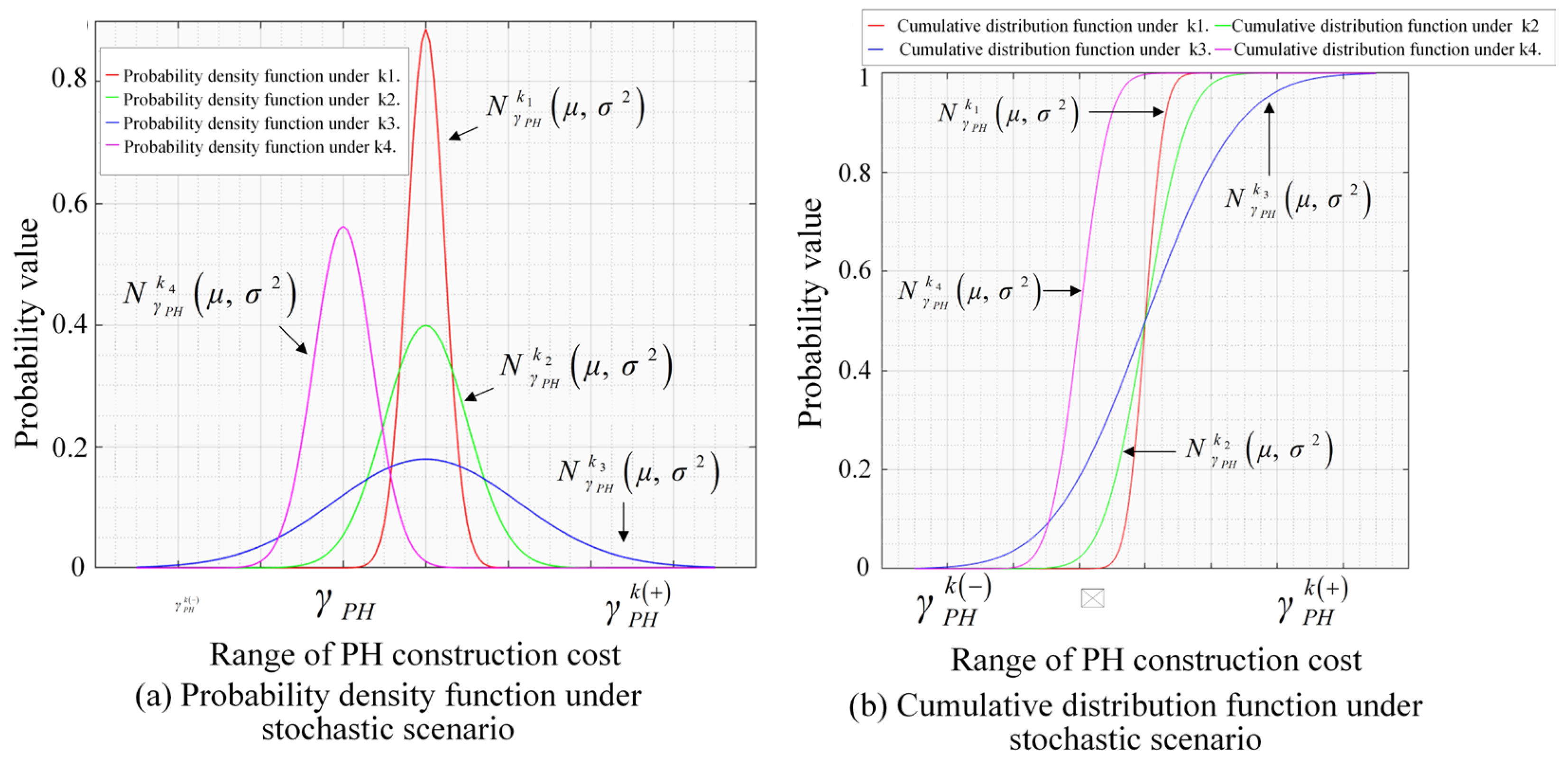
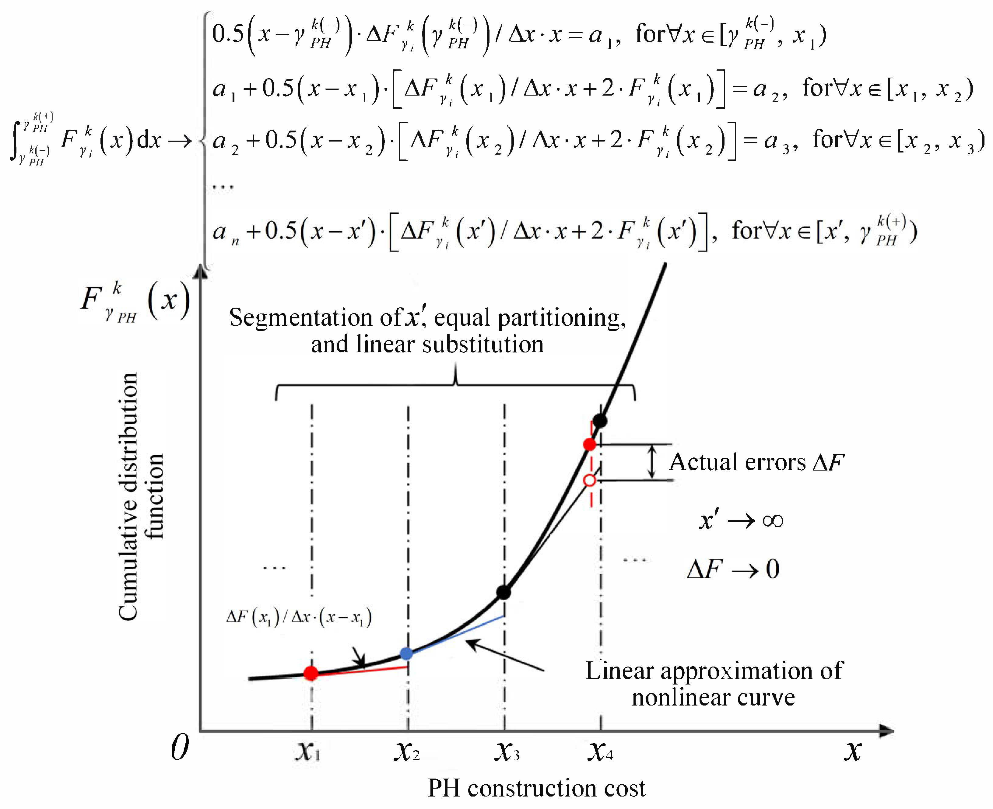
3.3.1. Approximation of Probability Distribution of Stochastic Variables

The optimization process of the stochastic robust model requires ensuring the “approximate optimality” of the optimization objective under any possible random scenario [40]. In other words, the model aims to obtain a comprehensive, approximately optimal feasible solution under all potential random scenarios. In the nonlinear mixed-integer programming model proposed in Section 3.3, in addition to the external constants and binary decision variables described in Table 1, there are two types of variables: (1) control variables and (2) stochastic variables, as shown in Table 2. Among them, the control variables are determined before the generation of stochastic parameters and cannot be adjusted after the stochastic parameters are generated. These variables control the robustness of the model and indirectly reflect the decision-maker’s attitude towards the design of the ULS network—whether it is conservative or risk-taking. A highly robust ULS network implies that more facilities are used to meet the potential demand, which could be higher than the predicted value. In contrast, a low-robustness ULS network tends to adopt a more risk-taking approach, assuming a low probability of actual demand exceeding the predicted value, and thus installs fewer facilities to reduce investment. These two objectives are opposing, representing two different optimization directions: profit maximization (low robustness) and risk minimization (high robustness). The decision-maker can make a choice based on their preferences and practical circumstances by adjusting the control variables, determining “how much profit they are willing to sacrifice for a more robust planning solution”.

In the robust objective function constructed above, it is necessary to first calculate the squared difference between the probability-weighted stochastic objective function and the stochastic objective function for each random scenario. To eliminate the nonlinearity in the model calculations, this study replaces the aforementioned “squared difference formulation” with a “standard deviation formulation”. The reconstructed model objective system is shown in Equation (33). Although the latter more precisely describes the degree of dispersion between solutions in different random scenarios and the baseline predicted scenario, which is beneficial for obtaining more realistic feedback from the model under robust conditions, the linearized form is clearly more suitable for the large and complex mathematical model in this study, considering the computational complexity.

$$\left\{\begin{array}{l}\min {\widehat{f}}_{\mathrm{robust}}^{\left(1\right)}=f_{\mathrm{random}}^{\left(1\right)\ast }-{\mathsf{\Gamma }}^{\left(1\right)}\cdot {\mathsf{\Omega }}_k\cdot \left[\left|f_{\mathrm{random}}^{\left(1\right)}\left(k_1\right)-f_{\mathrm{random}}^{\left(1\right)\ast }\right|+\cdots +\left|f_{\mathrm{random}}^{\left(1\right)}\left(k_n\right)-f_{\mathrm{random}}^{\left(1\right)\ast }\right|\right]\\ \min {\widehat{f}}_{\mathrm{robust}}^{\left(2\right)}=f_{\mathrm{random}}^{\left(2\right)\ast }-{\mathsf{\Gamma }}^{\left(2\right)}\cdot {\mathsf{\Omega }}_k\cdot \left[\left|f_{\mathrm{random}}^{\left(2\right)}\left(k_1\right)-f_{\mathrm{random}}^{\left(2\right)\ast }\right|+\cdots +\left|f_{\mathrm{random}}^{\left(2\right)}\left(k_n\right)-f_{\mathrm{random}}^{\left(2\right)\ast }\right|\right]\\ \min {\widehat{f}}_{\mathrm{robust}}^{\left(3\right)}=f_{\mathrm{random}}^{\left(3\right)\ast }-{\mathsf{\Gamma }}^{\left(3\right)}\cdot {\mathsf{\Omega }}_k\cdot \left[\left|f_{\mathrm{random}}^{\left(3\right)}\left(k_1\right)-f_{\mathrm{random}}^{\left(3\right)\ast }\right|+\cdots +\left|f_{\mathrm{random}}^{\left(3\right)}\left(k_n\right)-f_{\mathrm{random}}^{\left(3\right)\ast }\right|\right]\\ \min {\widehat{f}}_{\mathrm{robust}}^{\left(4\right)}=f_{\mathrm{random}}^{\left(4\right)\ast }-{\mathsf{\Gamma }}^{\left(4\right)}\cdot {\mathsf{\Omega }}_k\cdot \left[\left|f_{\mathrm{random}}^{\left(4\right)}\left(k_1\right)-f_{\mathrm{random}}^{\left(4\right)\ast }\right|+\cdots +\left|f_{\mathrm{random}}^{\left(4\right)}\left(k_n\right)-f_{\mathrm{random}}^{\left(4\right)\ast }\right|\right]\end{array}\right.$$

(33)

This paper assumes that the random variables in Table 1 have their respective probability density functions (as shown in Figure 4a), requiring the integration of the normal cumulative distribution function, which results in significant nonlinearity in the model (as shown in Figure 4b). Therefore, this paper proposes a numerical technique to linearize the integral function. For continuous nonlinear functions within the upper and lower bounds of the cumulative distribution function, the domain of the function is divided into a series of discrete intervals using piecewise linear transformations, and within each interval, the convex function is approximated by a straight line with a unique slope, as illustrated in Figure 5. Taking the cumulative distribution curve $F_{{\gamma }_{PH}}^k\left(x\right)$ of the hub node as an example, the range of the independent variable $\left[{\gamma }_{PH}^{k\left(-\right)}, {\gamma }_{PH}^{k\left(+\right)}\right]$ is divided into $x^{\prime }$ equal parts, and the function relationship between each pair of adjacent nodes can be approximated using a general linear form. By approximating the nonlinear model, the optimal solution of the linear model is obtained; however, this linearized model is not exactly the same as the nonlinear model. On the other hand, since the nonlinear model is convex, we obtain a solution close to the global optimum, but there is an error. As the number of intervals increases, the error decreases, and when $x^{\prime }$ tends to a very large number, the error $\Delta F$ approaches zero. Similar approximation methods are applied to all integral variables in the objective function and constraints of the model, resulting in a multi-objective mixed-integer linear programming model for the ULS network layout.

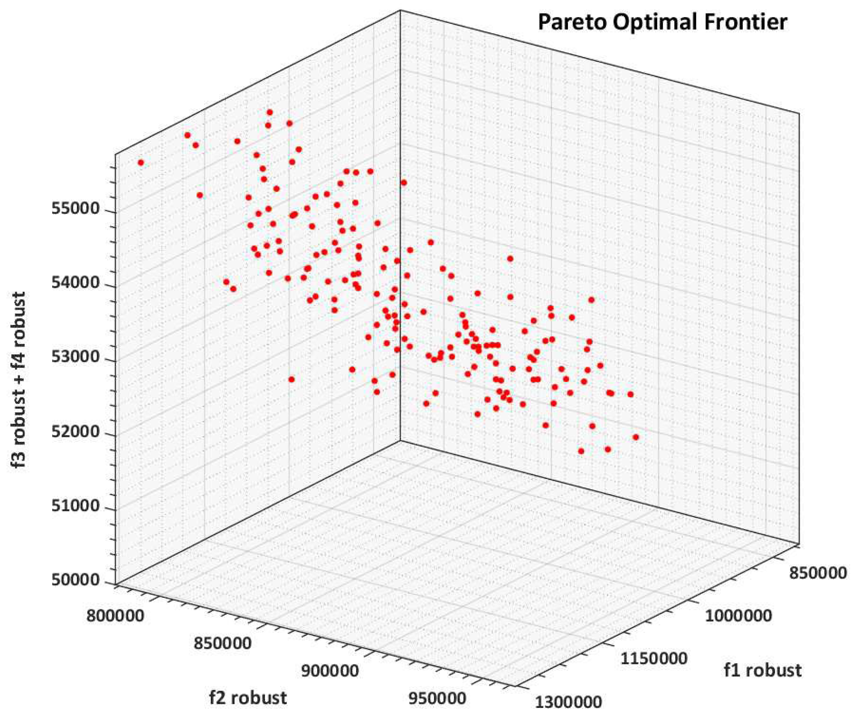
3.3.2. Pareto Fronts Normalized Weighting Method

Unlike optimization problems with a single objective function, urban ULS network planning in a complex environment involves at least four codependent (non-strictly opposing) sub-objectives. As a result, the model does not have a unique optimal solution. For multi-objective planning problems, an established and effective approach is to solve for as many Pareto-optimal solutions as possible [14], forming a Pareto-optimal solution set with good multidirectionality. This allows for the derivation of combined objective functions that are infinitely close to the Pareto front, based on the decision-maker’s preferences for each objective function (e.g., whether the ULS planning goal prioritizes construction cost savings or operational efficiency, etc.), as illustrated in Figure 6.

Classic methods for constructing Pareto solutions include function weighting, min-max methods, and the SEMOPS method. By setting appropriate weights for the objective functions, the multi-objective optimization problem is converted into a single-objective extreme value problem. This paper uses the function weighting method, where a set of weight factors $\left\{{\lambda }_1, {\lambda }_2, {\lambda }_3, {\lambda }_4\right\}$ linearly combine the sub-objective functions for the ULS network layout planning. Considering the differences in the scales of cost and efficiency in the objective functions, different degrees of amplification are applied to different sub-objective values when determining the weight factors. The reconstructed ULS network CLAR models under deterministic and random robust conditions are as follows, denoted as M-1 and M-2, respectively.

M-1 is the single-objective linear CLAR model considering random robustness, and its formula is as follows:

$$\mathrm{Minimize} Obj\left[\mathrm{M}\text{-}1\right]={\lambda }_1\times {\widehat{f}}_{\mathrm{robust}}^{\left(1\right)}+{\lambda }_2\times {\widehat{f}}_{\mathrm{robust}}^{\left(2\right)}+{\lambda }_3\times {\widehat{f}}_{\mathrm{robust}}^{\left(3\right)}+{\lambda }_4\times {\widehat{f}}_{\mathrm{robust}}^{\left(4\right)}$$

(34)

It is subject to the following: Constraints (15), (17), (19), (21), (23), and Constraints (24) to (32).

M-2 is the single-objective linear CLAR model under deterministic conditions, and its formula is as follows:

$$\mathrm{Minimize} Obj\left[\mathrm{M}\text{-}2\right]={\lambda }_1\times f_{\mathrm{determ}}^{\left(1\right)}+{\lambda }_2\times f_{\mathrm{determ}}^{\left(2\right)}+{\lambda }_3\times f_{\mathrm{determ}}^{\left(3\right)}+{\lambda }_4\times f_{\mathrm{determ}}^{\left(4\right)}$$

(35)

It is subject to the following: Constraints (14), (16), (18), (20), (22), and Constraints (24) to (32).

3.3.3. Model Complexity Analysis

It is evident that the restructured ULS network layout planning problem is a combinatorial variant of the classic two-echelon capacitated facility location–allocation problem (2E-CFLAP) and the multi-depot capacitated vehicle routing problem (MCVRP). The MCVRP can be considered as a subproblem, while the 2E-CFLAP serves as the main problem. Extensive research evidence indicates that both the MCVRP and 2E-CFLAP are NP-hard problems [41,42], meaning that their combination is also NP-hard. Even when solved separately, global optimal solutions cannot be obtained in polynomial time. The complexity of the restructured CLAR model is influenced by the scale of the ULS network planning case, including the number of logistics parks $‖S‖$, logistics aggregation points $‖J‖$, demand points $‖N‖$, and random scenarios $‖K‖$. For the case study of Beijing’s Fifth Ring District discussed in this paper, it is estimated that the total number of model constraints and decision variables for a single random scenario is close to 8 billion, as shown in

Table 3. Calculation magnitude of decision variables and constraints in reformulated CLAR model.

Variables and Constraints	Maximum Quantity Expression	Beijing Case
$A_i^k$, $B_j^k$, Equations (15), (17), (19) and (30)	$3\times ‖N‖+5\times ‖J‖$	4018
${\phi }_p^k$, ${\rho }_q^k$, Equation (23)	$2\times ‖N‖\times ‖J‖+P_{‖J‖}^2$	689,022
${\xi }_g^k$, ${\zeta }_h^k$, Equation (21)	$‖S‖\times ‖N‖+3\times C_{‖N‖}^2$	8930
Equations (25), (26) and (31)	$7\times ‖S‖\times ‖J‖+‖S‖+‖J‖+P_{‖N‖}^2$	32,993
$X_{sij}^k$, $Z_{sij}^k$, Equation (27)	$3\times ‖S‖\times ‖J‖\times ‖N‖$	864,120
$R_{sjp}^k$, $T_{sjq}^k$, $M_{sjq}^k$, ${\varsigma }_{sjp}^k$, Equations (24), (27)–(29)	$6\times ‖S‖\times ‖J‖\times \left(‖N‖\times ‖J‖+C_{‖J‖}^2\right)$	7,833,952,740
$U_{sjg}^k$, $V_{sjh}^k$, Equation (28)	$2\times ‖S‖\times ‖J‖\times \left(‖S‖\times ‖N‖+C_{‖N‖}^2\right)$	46,086,400
$Y_{sj{j}^{\prime }}^k$, $W_{i{i}^{\prime }h}^k$, Equations (27) and (28)	$3\times P_{‖N‖}^2\times C_{‖N‖}^2+2\times ‖S‖\times P_{‖J‖}^2$	54,473,060
Total number		7,936,111,283

.

Moreover, the increase in the number of facilities and the scale of the two types of O-D matrices results in an exponential growth in computational complexity. Clearly, conventional exact algorithms (e.g., branch-and-bound methods) or linear programming solvers (e.g., CPLEX and LINGO) struggle to obtain a global optimal solution for such a large-scale model within a reasonable computational time. In contrast, meta-heuristic techniques exhibit significant advantages in improving computational efficiency and obtaining high-quality approximate optimal solutions [43]. Heuristic optimization algorithms do not rely on problem-specific gradient information or other structural properties, making them more robust to increasing complexity in terms of the number of variables, dimensions, and problem convexity. To address the ULS network layout optimization problem under complex scenarios, this study proposes an improved multi-objective particle swarm optimization algorithm based on immune selection (IS-MPSO).

4. Solution Approach

Particle swarm optimization (PSO) is a global stochastic search algorithm based on swarm intelligence, inspired by the migration and aggregation behaviors observed in bird foraging. It was first proposed in 1995 by American social psychologist James Kennedy and electrical engineer Russell Eberhart [44].

In the PSO algorithm, the i particle is represented as $R_i$, and the particle swarm consisting of N particles is denoted as $R=(R_1,R_2,\cdots ,R_i,\cdots ,R_N)$. At time t, the position, velocity, and fitness value of particle EEE are represented as $P_i(t)={(x{1}_i(t),x{2}_i(t),\cdots ,x{n}_i(t))}^T$, $V_i(t)={(v_{ix1}(t),v_{ix2}(t),\cdots ,v_{ixn}(t))}^T$, and $c_i(t)$, respectively. The fitness value of a particle is determined by the objective function value at its current position. During the search for the optimal solution, once a particle discovers a superior solution, other particles adjust their positions accordingly by following the PSO algorithm to converge toward the location of the optimal particle.

Although the PSO algorithm exhibits strong global optimization capabilities and fast convergence speed, it is prone to premature convergence, leading to suboptimal solutions and a loss of diversity in the Pareto-optimal set. The PSO algorithm requires the assignment of certain prior preferences to guide the selection process. Therefore, when applying PSO to multi-objective optimization problems, it is essential to enhance its local search capability and global search efficiency to improve its performance. These improvements are necessary for effectively solving the complex multi-objective optimization model for urban ULS network layout planning. The modifications to the traditional PSO algorithm proposed in this study are elaborated as follows.

(1) Global best and personal best update mechanism.

In single-objective PSO, the fitness value of each particle is unique and they can be directly compared. However, in a multi-objective optimization model, the solutions within the Pareto-optimal set exhibit a nondominant relationship, meaning that no single solution is strictly superior to others. Therefore, a new selection strategy is required to determine the global best and personal best solutions from the particle swarm.

To ensure diversity in the Pareto-optimal set of a multi-objective optimization model, the update mechanism for both the global best and personal best solutions must account for the multidirectional nature of the Pareto front. Depending on the characteristics of each particle, the corresponding global best and personal best solutions should be selected dynamically. Assuming that at time t, the Pareto-optimal set (global optimal set) of the ULS network layout multi-objective optimization model is denoted as $R1=\left\{R{1}_1,R{1}_2,\cdots ,R{1}_{n_1}\right\}$, the global best selection strategy for particle $R_i$ is formulated as follows:

$$s_{(R_i, R{1}_k)}=\underset{j\in \left\{1,2,\cdots ,n_1\right\}}{\min } s(R_i, R{1}_j)=\underset{j\in \left\{1,2,\cdots ,n_1\right\}}{\min }\arccos {\displaystyle \frac{{\overrightarrow{c}}_i(t)\cdot {\overrightarrow{c}}_j(t)}{\left|{\overrightarrow{c}}_i(t)\right|\cdot \left|{\overrightarrow{c}}_j(t)\right|}}$$

(36)

where ${\overrightarrow{c}}_i(t)=\left(c_i^1(t),c_i^2(t)\cdots ,c_i^{n_2}(t)\right)$ represents the fitness vector of particle $R_i$; $n_2$ denotes the number of objective functions in the model; and $s(R_i, R{1}_j)$ represents the angle between the fitness vector of particle $R_i$ and that of particle $R{1}_j$ in the Pareto-optimal set. The position of particle $R{1}_k$ within the Pareto-optimal set is selected as the global best position for updating particle $R_i$. Thus, each particle $R_i$ selects a global best particle $R{1}_j$ from the Pareto-optimal set. The number of particles $R_i$ in the swarm that correspond to each global best particle $R_i$ is referred to as the particle concentration $n_{R{1}_j}$.

(2) Optimization methods for local and global search.

To ensure that particles do not repeatedly traverse the search space within a certain range and to prevent convergence to suboptimal local solutions, a local search strategy for the multi-objective particle swarm optimization (MOPSO) algorithm can be designed as follows:

Step 1: Set the iteration count $n_4$. At the start of the local search, initialize the iteration count as $It=It+1$. The position $x{k}_i(It)$ transformation formula for particle $R_i$ at position $P_i(It)={(x{1}_i(It),x{2}_i(It),\cdots ,x{k}_i(It),\cdots ,x{n}_i(It))}^T$ is given as follows:

$$x{k}_i(It+1)=x{k}_{\min ,i}+4\cdot {\displaystyle \frac{x{k}_i(It)-x{k}_{\min ,i}}{x{k}_i(It)-x{k}_{\max ,i}}}(1-{\displaystyle \frac{x{k}_i(It)-x{k}_{\min ,i}}{x{k}_i(It)-x{k}_{\max ,i}}})(x{k}_{\max ,i}-x{k}_{\min ,i})$$

(37)

where $x{k}_{\min ,i}$ and $x{k}_{\max ,i}$ represent the lower and upper bounds of the search region for $x{k}_i(It)$, respectively. Through transformation, the position of particle $P_i(It+1)$ is updated to $P_i(It+1)$. If the fitness value of $P_i(It)$ is superior to that of $It=n_4$, or if the iteration count reaches III, proceed to Step 3; otherwise, continue to Step 2.

Step 2: Update $x{k}_{\min ,i}$ and $x{k}_{\max ,i}$ to dynamically adjust the search region, maintaining the characteristics of particle diversity and dispersion. Based on the selected global optimal particle $R{1}_j$, the lower bound $x{k}_{\min ,i}$ and upper bound $x{k}_{\max ,i}$ of its search region are determined by Equations (38) and (39). Here, $a_2$ is a random number within the range [0, 1].

$$x{k}_{\min ,i}=\max \{x{k}_{\min ,i},x{k}_{gj,i}-a_2\cdot (x{k}_{\max ,i}-x{k}_{\min ,i})\}$$

(38)

$$x{k}_{\max ,i}=\max \{x{k}_{\max ,i},x{k}_{gj,i}+a_2\cdot (x{k}_{\max ,i}-x{k}_{\min ,i})\}$$

(39)

Step 3: Update the particle’s position, individual historical best, and global best following the global and individual historical best update method. After completing the local search, return to the main PSO algorithm. To enhance particle diversity, improve search capability in the early stages, and accelerate convergence in later stages, this study incorporates an immune-selection-based particle crossover operation to prevent premature convergence [45]. To ensure that the offspring particles of $R_i$ remain within the feasible solution space after crossover, the feasible transport path set is used to determine the permissible crossover positions of particle $R_i$, from which a position is randomly selected. In this study, the antibody concentration of a particle is adopted as the crossover selection probability. The probability of selecting particle $R_i$ for crossover is given by the following equation:

$$PB(R_i)={\displaystyle \frac{1}{N}}{e}^{-u\cdot {{\displaystyle \sum _{k=1}^N(\left|{\overrightarrow{c}}_i(t)\right|-\left|{\overrightarrow{c}}_k(t)\right|)}}^{-1}}$$

(40)

Here, $\mu$ represents the constant adjustment factor, taking values between 0 and 1.

Additionally, to prevent particles that are too close to each other from crossing over and reducing the probability of generating better particles, the proximity of parent particles is assessed by calculating the Euclidean distance. Crossover is allowed only if the Euclidean distance between particles $R_i$ and $R_k$ exceeds the threshold $D_a$ Otherwise, particle $R_k$ is discarded, and a new particle is randomly generated until the condition is met. This logic can be expressed as follows:

$$D_{ij}(t)={‖P_i(t)-P_j(t)‖}_2={\left({(x{1}_i(t)-x{1}_j(t))}^2+\cdots +{(x{n}_i(t)-x{n}_j(t))}^2\right)}^{{\displaystyle \frac{1}{2}}}$$

(41)

5. Case Study

5.1. Simulation Scenarios

Based on the Beijing case presented [26], a simulation scenario for the urban ULS network layout planning was constructed. Firstly, the peak year 2035 was selected for the ULS network planning, and the total demand for the conceptual ULS was allocated by land parcels, resulting in the “forward freight O-D matrix” and the “same-city delivery O-D matrix”. Secondly, drawing from primary data on global ULS planning [26], supplemented by expert surveys, the values for constant parameters in the mathematical model were defined. The goal was to ensure the objectivity and authenticity of key parameters (such as the construction cost of underground tunnels, capacity, transportation system parameters, impact factors related to benefits, and node coverage radius), thereby enhancing the explanatory power of the simulation results for real-world problems. For uncertain parameters in the model under stochastic conditions, the characteristic values (including variance of normal distribution, probability density functions, and robust control coefficients) were randomly defined within the variable range of the parameter predictions. This ensured that feasible solutions existed when the variables took values at the upper and lower bounds of the predicted range, while also reflecting the uncertainty level in real-world ULS network planning.

Table 4. Exogenous data and predicted variable value for Beijing ULS network layout planning.

Parameters	Value	Parameters	Value
${\upsilon }_{PT}$	CNY 0.5 × 107/km	${\epsilon }_{PT}$	0.7
${\upsilon }_{ST}$	CNY 0.14 × 107/km	${\epsilon }_{ST}$	0.6
$\mathsf{\alpha }$	CNY 2 per 103 parcel km	${\eta }_{PT}$	CNY 10 per 103 parcel
$\mathsf{\beta }$	CNY 8 per 103 parcel km	${\eta }_{ST}$	CNY 5 per 103 parcel
c	CNY 10 per 103 parcel km	ro	3 km
${\gamma }_{PH}$	CNY 1 × 107	${\tau }_{PT}$	60 km/h
${\gamma }_{SN}$	CNY 0.35 × 107	${\tau }_{ST}$	30 km/h
[cap1]	30 × 104 parcel/d	${\tau }_{LMD}$	10 km/h
[cap2]	7 × 104 parcel/d	${\omega }_{PH}$	40 min
[cap3]	7 × 104 parcel/d	${\omega }_{SN}$	20 min
[cap4]	60 × 104 parcel/d	$\theta$	70 × 365 d
[cap5]	30 × 104 parcel/d	Objective function weights	[1, 1.2, 0.03, 10]

presents the baseline constant parameter values employed in planning the ULS network layout for the study area. Under stochastic conditions, the corresponding characteristic values of the variables are provided in

Table 5. Robustness control parameters and eigenvalues of stochastic variables.

Variable	1	2	3	4	5	6	7	8
$d_{sj}$	[0,0.85]	[0,1.96]	[0,1.13]	[0,2.48]	[0,1.91]	[0,2.15]	[0,1.49]	[0,1.34]
${\delta }_{i{i}^{\prime }}$	[0,0.14]	[0,0.16]	[0, 0.2]	[0,0.03]	[0,0.23]	[0,0.38]	[0,0.12]	[0,0.09]
${\gamma }_{PH}$	950	1199	5389	65,524	30,999	422	8391	26,804
${\gamma }_{SN}$	270	11,919	12,467	42,230	7926	248	2748	34,715
${\upsilon }_{PT}$	670	31,119	6638	670	26,988	15,288	9644	8602
${\upsilon }_{ST}$	8225	6578	114	1288	17,660	103	92	24
$\mathsf{\alpha }$	0.10	0.84	0.67	0.80	1.49	0.98	0.97	0.33
$\mathsf{\beta }$	11.80	5.25	1.28	0.11	10.32	0.10	3.80	12.80
${\omega }_{PH}$	72,253	43,718	51,495	52,706	36,000	17,424	12,617	23,963
${\omega }_{SN}$	88,744	2916	55,319	16,697	4679	14,175	70,671	20,736
${\mathsf{\Omega }}_k$	0.247	0.165	0.091	0.113	0.142	0.067	0.084	0.091
${\mathsf{\Gamma }}^{\left(1\right)}$	1.117 1.095 0.898 0.941

.

The experiments were conducted on a Python 3.8 (32-bit) platform with an Intel Core i9-9900K CPU @ 4.50 GHz and 64 GB RAM. The parameter settings for the improved multi-objective PSO algorithm with immune selection were as follows: learning factors c₁ = c₂ = 1.5; inertia weight ${\theta }_{\max }$ = 0.9 (initial) and ${\theta }_{\min }$ = 0.4 (final); cloning ratio, 30%; roulette selection probability, 85%; population size N = 200; and maximum number of iterations MaxGen = 500.

The heuristic algorithm was executed 20 times, and the weighted average total objective value under the stochastic robust scenario was obtained. The IS-MPSO algorithm effectively reduced the total objective function from 9.8 × 10⁶ to an approximately optimal value of 3.4 × 10⁶ within 500 iterations, demonstrating significant optimization performance. During the 20 independent runs, the algorithm converged on average after 280 iterations. The total CPU time required for the 20 optimization runs was 19,568 s, significantly outperforming exact algorithms in solving problems of similar complexity, as shown in

Table 6. Performance comparison of IS-MPSO and traditional PSO across test networks.

Algorithms	Traditional PSO	IS-MPSO
Network cost reduction ratio	38%	62%
Average number of convergence iterations	420	280
CPU time	64,356 s	19,568 s

.

The Pareto-optimal front distribution of the sub-objective function values under the stochastic robust scenario is illustrated in Figure 7. It is evident that the IS-MPSO algorithm effectively synchronizes the optimization of the four sub-objectives in Model M-1. As shown in Figure 7, after 500 iterations of velocity and position updates, the particle swarm (with a population size of 200) stabilized within a compact solution space, highlighting the stability of the proposed algorithm and its ability to efficiently obtain high-quality solutions.

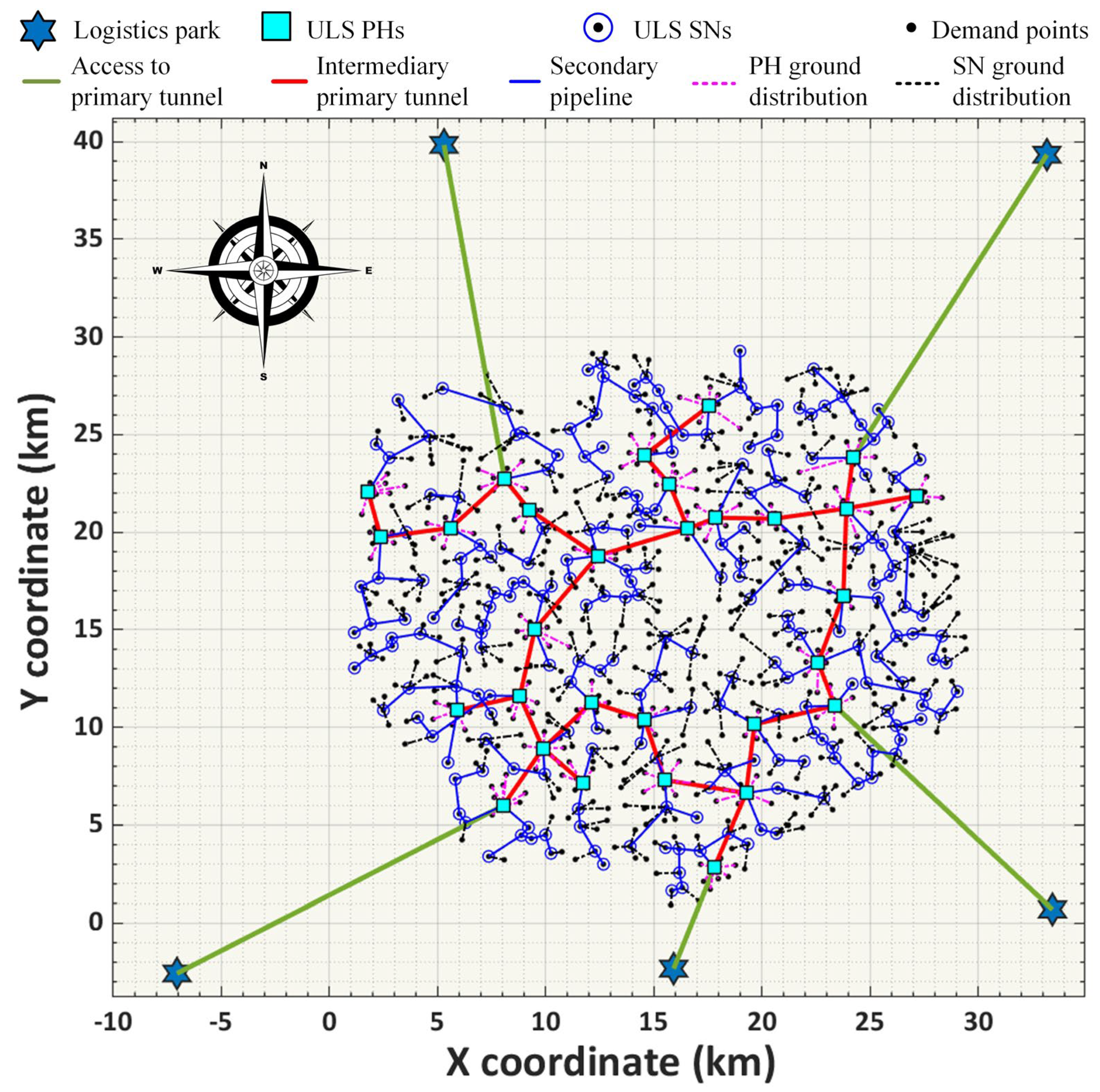
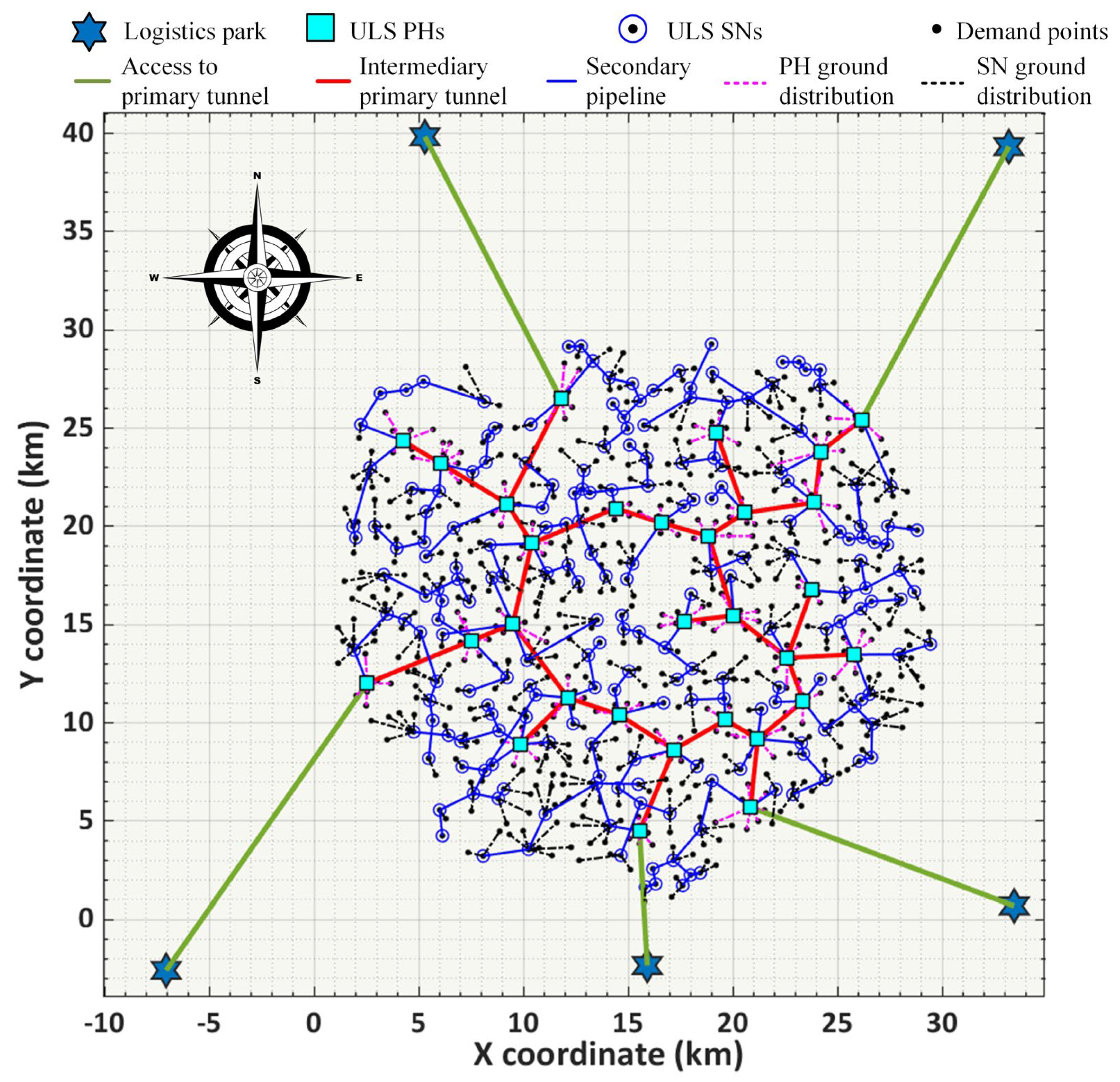
5.2. Comparison of Optimal ULS Layouts

The optimal ULS network layouts under the baseline scenario and stochastic robust scenario are illustrated in Figure 8 and Figure 9, respectively. The macroscopic network configuration schemes for both scenarios are summarized in

Table 7. Overview of optimal ULS network configurations under two scenarios.

	Random Robust Scenario (Model M-1)	Baseline Scenario (Model M-2)
Total objective function value	$Obj\left[\mathrm{M}\text{-}1\right]$ = 3.4 × 106	$Obj\left[\mathrm{M}\text{-}2\right]$ = 3.6 × 106
Sub-objective 1	${\widehat{f}}_{\mathrm{robust}}^{\left(1\right)}$ = 118.9 × 104 CNY	$f_{\mathrm{determ}}^{\left(1\right)}$ = 116.7 × 104 CNY
Sub-objective 2	${\widehat{f}}_{\mathrm{robust}}^{\left(2\right)}$ = 86.7 × 104 CNY	$f_{\mathrm{determ}}^{\left(2\right)}$ = 96.9 × 104 CNY
Sub-objective 3	${\widehat{f}}_{\mathrm{robust}}^{\left(3\right)}$ = 2083.2 s	$f_{\mathrm{determ}}^{\left(3\right)}$ = 2037.2 s
Sub-objective 4	${\widehat{f}}_{\mathrm{robust}}^{\left(4\right)}$ = 5.1 × 104 CNY	$f_{\mathrm{determ}}^{\left(4\right)}$ = 6.4 × 104 CNY
Number of HNs	30	30
Number of SNs	204	220
Total length of first-tier tunnels	137 km	144 km
Total length of second-tier pipelines	774 km	851 km
Average end-point ground delivery length of nodes	1.13 km	0.94 km
Average load rate of first-tier tunnels	58.83%	45.14%
Average load rate of second-tier pipelines	40.29%	36.88%
Average ground transport volume at HNs	6.64 × 104 parcels	6.54 × 104 parcels
Average underground transport volume at HNs	19.47 × 104 parcels	19.58 × 104 parcels
Average ground transport volume at SNs	2.88 × 104 parcels	2.7 × 104 parcels
Average travel distance of forward O-D on first-tier and second-tier networks	28.72 km, 3.98 km	32.49 km, 4.27 km
Average travel distance of same-city O-D on first-tier network	15.59 km	17.16 km
Ground freight mitigation rate by ULS	RFAR = 98.14%	RFAR = 97.14%
Greenhouse gas reducing service	1.82 × 105 CNY/year	2.02 × 105 CNY/year
Air pollution reducing service	1.73 × 104 CNY/year	1.95 × 104 CNY/year

.

The optimal objective function values for the stochastic robust model (M-1) and the deterministic model (M-2) are 3.4 × 10⁶ and 3.6 × 10⁶, respectively. In M-1, the sub-objectives under the stochastic robust scenario include the following: Depreciation of total ULS network construction cost: 1.19 million CNY/day. ULS network transportation cost: 0.87 million CNY/day. System operational efficiency (average transport time of forward O-D orders, non-actual value): 2083 s. Channel load level (underutilization penalty cost): 0.05 million CNY/day. For M-2, the corresponding sub-objectives are as follows: Depreciation of total ULS network construction cost: 1.17 million CNY/day. ULS network transportation cost: 0.97 million CNY/day. System operational efficiency: 2037 s. Channel load level: 0.06 million CNY/day. Under the stochastic robust scenario, the ULS network in Beijing’s Fifth Ring Road area consists of 30 hub nodes and 204 spoke nodes. The primary tunnel network has a total length of 137 km, with an average load factor of 59%, while the secondary pipeline network extends 774 km, with an average load factor of 40%. For last-mile ground delivery, the average parcel volume handled at hub and spoke nodes is 66,000 parcels/day and 29,000 parcels/day, respectively. The average last-mile delivery distance from ULS nodes to customers is 1.1 km. Each hub node processes an average of 195,000 parcels/day for secondary underground transportation. The average transport distance per forward O-D in the primary and secondary ULS networks is 28.7 km and 4 km, respectively. The average transport distance per intra-city O-D in the primary network is 15.6 km.

According to [25], the Relief Factor of Urban Freight Traffic (RFAR) for the ULS was calculated as the ratio of the difference between freight traffic volume under the conventional logistics model and the surface-level last-mile delivery traffic volume in the ULS network to the former. In the Beijing ULS planning case presented in this section, the RFAR values under the two scenarios were 98.1% and 97.1%, respectively. These results indicate that the ULS network can effectively eliminate the travel trajectories of small- and medium-sized logistics vehicles within urban areas, significantly alleviating traffic congestion and enhancing environmental benefits. According to Pan et al. (2023) [46], the ULS generates economic benefits of approximately 2.22 × 10⁵ CNY/year for greenhouse gas emission reductions and 1.99 × 10⁵ CNY/year for reductions in air pollutant emissions.

These results indicate that, compared to the baseline scenario, the randomly robust ULS network layout features the same number of hub nodes but fewer spoke nodes, a shorter total length of primary tunnels, and a reduced total length of secondary pipelines. Both network configurations exhibit similar performance in terms of channel facility utilization, urban freight traffic relief, and underground transport ratio. However, freight O-D pairs in the randomly robust network experience shorter underground transport distances. From a network topology perspective, the optimal layouts of the primary ULS network in both scenarios exhibit a “ring structure” with multiple “synapse-like” extensions. Specifically, a primary tunnel ring is formed between the hub nodes surrounding the urban center, facilitating the centralized collection of incoming freight from peripheral hubs for efficient turnover. The key difference lies in the ring size and location. In the randomly robust scenario, the primary tunnel ring is shorter and located between Beijing’s Third and Fourth Ring Roads. In contrast, in the baseline scenario, the ring extends further southeast, with over half of its tunnel segments distributed between the Fourth and Fifth Ring Roads. Extending outward from the tunnel ring, “synapse-like” tunnel segments enable the primary ULS network to serve urban areas beyond the ring structure. The randomly robust scenario features more synaptic tunnel branches than the baseline case. Regarding the secondary pipeline network topology, both scenarios predominantly exhibit a “single-tree” or “multi-branch tree” structure. The largest spanning tree in the secondary network connects nine spoke nodes in the randomly robust scenario, compared to eleven in the baseline scenario. Meanwhile, the smallest spanning tree in both networks consists of only one node, reflecting significant variations in the density of underground distribution tasks at hub nodes, necessitating an efficient allocation of logistics resources within hubs.

To further analyze the optimal ULS network, the 30 hub nodes were used as reference points to segment the network. Regarding transportation costs, the highest first-tier network travel cost was observed for forward O-D shipments destined for hub node PH-53, with a daily transportation cost of CNY 30,300. Within the PH-63 region, the secondary pipeline network and the last-mile ground delivery network incurred the highest transportation costs, reaching 9500 CNY/day and 9000 CNY/day, respectively. PH-59 has the largest number of affiliated spoke nodes (13). PH-22, PH-47, and PH-63 cover the highest number of demand points, each serving 36 locations. The longest secondary pipeline spans 52.66 km, whereas the shortest measures only 3.04 km. The last-mile delivery distance between spoke or hub nodes and demand points range from 520 m to 1270 m. In terms of transportation time, the travel time for forward O-D freight from logistics parks to hub nodes ranges from 15 to 22.3 min. The travel time from hub nodes to spoke nodes falls within 7.1 to 10.5 min. The last-mile ground transportation time varies between 4.3 and 6.3 min.

5.3. Sensitivity Analysis

By adjusting the transport capacity of the intermediary first-tier tunnels [cap4] and the freight rate for goods transported through the first-tier tunnels, the impact of key parameter variations on the optimal network layout was analyzed. Specifically, the baseline value of [cap4] was scaled at 40%, 60%, 85%, 100%, 120%, 150%, and 200% to create different levels of adjustment. Similarly, these variations formed two sets of “perturbation scenarios”. Unlike the small-range probability distribution of parameters in the randomly robust scenario, the perturbation scenarios introduce greater variations in parameter values. The primary objective was to assess the model’s sensitivity to external parameter settings, thereby providing a reference for selecting reasonable parameter ranges in ULS network planning. Except for the two adjusted parameters, all other parameter values in the perturbation scenarios remained consistent with those in the baseline scenario.

Table 8. Impact of PT capacity on optimal network configuration.

[cap4] Perturbation Range	40%	60%	85%	100%	120%	150%	200%
Construction cost (CNY × 104/d)	127.2	121.6	116.4	116.7	114.5	112.7	110.1
Transport cost (CNY × 104/d)	100.7	99.7	97.2	96.9	95.5	92.1	89.4
System efficiency (s)	2088	2040	2052	2034	1992	1974	1926
Penalty cost (CNY × 104/d)	3.9	4.4	5.6	6.4	8	8.9	10.1
Average load of first-tier tunnels	86%	70%	52%	45%	41%	37%	30%
First-tier network length (km)	173	160	148	144	140	135	132
Second-tier network length (km)	863	856	844	851	843	840	832
Number of HNs	37	33	30	30	29	28	26
Number of SNs	230	222	215	220	216	214	208
Total objective value of Model M-2	3.4 × 106	3.4 × 106	3.5 × 106	3.6 × 106	3.7 × 106	3.7 × 106	3.8 × 106

presents the impact of [cap4] parameter variations on the optimal ULS network configuration. The results indicate that the transport capacity of first-tier tunnels primarily affects the number of hub nodes, the length of the first-tier network, construction costs (sub-objective 1), and tunnel load levels (sub-objective 4). As [cap4] decreases from 200% to 40% of its baseline value, sub-objective 1 of Model M-2 increases from 1.1 million CNY/day to 1.27 million CNY/day, the average load rate of first-tier tunnels rises from 30% to 86%, and the first-tier network length extends from 132 km to 173 km. Consequently, the total objective value of Model M-2 decreases from 3.8 × 10⁶ to 3.4 × 10⁶. On the other hand, as shown in

Table 9. Impact of unit underground transport cost on optimal network configuration.

$\mathit{\alpha }$ Perturbation Range	40%	60%	85%	100%	120%	150%	200%
Construction cost (CNY × 104/d)	118.5	118.2	116.5	116.7	117.0	117.3	116.4
Transport cost (CNY × 104/d)	50.7	68.1	86.3	96.9	112.8	139.3	183.6
System efficiency (s)	2070	2064	2052	2034	2004	1986	1968
Penalty cost (CNY × 104/d)	7	6.9	6.7	6.4	6.2	5.9	5.6
Average load of first-tier tunnels	40%	43%	44%	45%	46%	47%	45%
First-tier network length (km)	160	153	147	144	142	140	136
Second-tier network length (km)	842	850	844	851	856	858	861
Number of HNs	33	32	30	30	29	29	27
Number of SNs	205	213	217	220	226	230	234
Total objective value of Model M-2	3.1 × 106	3.3 × 106	3.5 × 106	3.6 × 106	3.7 × 106	4 × 106	4.5 × 106

, a reduction in [cap4] leads to an increase in first-tier network length and the number of hub nodes, while simultaneously reducing system operational efficiency. However, other network configuration factors, such as construction costs, tunnel load, the number of spoke nodes, and second-tier network length, exhibit low sensitivity to variations in the first-tier network transport rate.

6. Conclusions

This study presents a robust, immune-inspired multi-objective optimization framework for hub-and-spoke underground logistics systems (ULSs) that is tailored to the complex demands of smart city planning and sustainable urban development. By integrating immune-inspired mechanisms with multi-objective particle swarm optimization (IS-MPSO), we propose a novel framework to solve the stochastic robust CLAR problem. The model simultaneously minimizes construction and operational costs, maximizes system efficiency, and enhances underground corridor utilization, while accounting for multidimensional uncertainties in demand, costs, and processing times. A case study of Beijing’s Fifth Ring District validates the model’s applicability in high-density urban environments, demonstrating its capability to balance robustness and economic efficiency.

The results highlight three major advancements:

(1) Algorithmic innovation: The IS-MPSO algorithm effectively resolves premature convergence issues in traditional PSO by introducing immune selection and dynamic search strategies. Compared with the baseline scenarios without stochastic perturbations, IS-MPSO achieves an average 62% reduction in total network cost and converges stably within 280 iterations on average.

(2) Modeling breakthrough: The proposed stochastic robust CLAR model integrates four hierarchical network layers (logistics parks, primary hubs, secondary hubs, and spoke nodes) and addresses eight decision variables, outperforming conventional two-echelon models in scalability and realism. The hybrid “ring–synapse” topology reduces last-mile delivery distances to 1.1 km, achieving a 98.1% relief in surface freight traffic (RFAR).

(3) Practical insights: The optimized ULS layout delivers tangible environmental and economic benefits: tunnel construction length is reduced to 137 km (from 144 km in the baseline), while corridor load utilization increases to 59% (versus 45%). These improvements not only support the low-carbon objectives of sustainable urban development but also offer actionable guidance for urban planners seeking to integrate underground space logistics into smart city infrastructure—striking an optimal balance between capital investment, operational resilience, and ecological stewardship.

Despite its contributions, this study has limitations. First, the model assumes deterministic tunnel connections and excludes geological constraints, which may affect real-world feasibility. Second, the computational complexity of handling 8 billion variables restricts its direct application to larger metropolitan regions. Future research should focus on the following developments: First, incorporating real-time scheduling and demand-responsive routing to enhance system flexibility. Second, multimodal integration, exploring synergies between ULSs and urban rail transit or autonomous delivery systems. Third, extended robustness, embedding scenario generation techniques (e.g., deep learning-based demand forecasting) to refine uncertainty modeling. Finally, integrating a multidimensional global sensitivity analysis into our existing framework, encompassing key parameters such as tunnel capacity, demand variability, and handling efficiency, to further enhance the model’s robustness and decision-support value.

These extensions will further bridge the gap between theoretical optimization and practical implementation, advancing sustainable urban logistics in the era of smart cities.

References

1. Gardrat, M. Urban growth and freight transport: From sprawl to distension. J. Transp. Geogr. 2021, 91, 102979. [Google Scholar] [CrossRef]
2. Chen, Z.; Dong, J.; Ren, R. Urban underground logistics system in China: Opportunities or challenges? Undergr. Space 2017, 2, 195–208. [Google Scholar] [CrossRef]
3. Zhou, Y.; Zhao, J. Assessment and planning of underground space use in Singapore. Tunn. Undergr. Space Technol. 2016, 55, 249–256. [Google Scholar] [CrossRef]
4. Di, Z.; Li, L.; Li, M.; Zhang, S.; Yan, Y.; Wang, M.; Li, B. Research on the contribution of metro-based freight to reducing urban transportation exhaust emissions. Comput. Ind. Eng. 2023, 185, 109622. [Google Scholar] [CrossRef]
5. Hou, L.; Xu, Y.; Ren, R.; Yang, J.; Su, L. Optimization of three-dimensional urban underground logistics system alignment: A deep reinforcement learning approach. Comput. Ind. Eng. 2025, 205, 111185. [Google Scholar] [CrossRef]
6. Shahooei, S.; Farooghi, F.; Zahedzahedani, S.E.; Shahandashti, M.; Ardekani, S. Application of underground short-haul freight pipelines to large airports. J. Air Transp. Manag. 2018, 71, 64–72. [Google Scholar] [CrossRef]
7. Hai, D.; Xu, J.; Duan, Z.; Chen, C. Effects of underground logistics system on urban freight traffic: A case study in Shanghai, China. J. Clean. Prod. 2020, 260, 121019. [Google Scholar] [CrossRef]
8. Dong, J.; Hu, W.; Yan, S.; Ren, R.; Zhao, X. Network Planning Method for Capacitated Metro-Based Underground Logistics System. Adv. Civ. Eng. 2018, 2018, 6958086. [Google Scholar] [CrossRef]
9. An, N.; Yang, K.; Chen, Y.; Yang, L. Wasserstein distributionally robust optimization for train operation and freight assignment in a metro-based underground logistics system. Comput. Ind. Eng. 2024, 192, 110228. [Google Scholar] [CrossRef]
10. He, R.; Bian, R.; Hua, J.; Zhao, L.; Xu, F.; Long, J. Multi-objective optimization of gasoline blending scheduling via NSGA-II algorithm with composite operators considering oil movement path planning. Expert Syst. Appl. 2025, 280, 127426. [Google Scholar] [CrossRef]
11. Luo, J.; Gu, Q.; Chen, L.; Li, X.; Li, P. Multi-objective optimization for ore blending schemes in the open-pit phosphate mine using an improved NSGA-II algorithm. Green Smart Min. Eng. 2025, 2, 42–56. [Google Scholar] [CrossRef]
12. Zhao, L.; Zhou, J.; Li, H.; Yang, P.; Zhou, L. Optimizing the design of an intra-city metro logistics system based on a hub-and-spoke network model. Tunn. Undergr. Space Technol. 2021, 116, 104086. [Google Scholar] [CrossRef]
13. Li, F.; Yuen, K.F. A systematic review on underground logistics system: Designs, impacts, and future directions. Tunn. Undergr. Space Technol. 2025, 159, 106483. [Google Scholar] [CrossRef]
14. Li, S.; Zhu, X.; Shang, P.; Wang, L.; Li, T. Scheduling shared passenger and freight transport for an underground logistics system. Transp. Res. Part B Methodol. 2024, 183, 102907. [Google Scholar] [CrossRef]
15. Baghalian, A.; Rezapour, S.; Farahani, R.Z. Robust supply chain network design with service level against disruptions and demand uncertainties: A real-life case. Eur. J. Oper. Res. 2013, 227, 199–215. [Google Scholar] [CrossRef]
16. Zhang, H.; Zhang, J.; Zheng, C.; Wang, B.; Chen, J. Node location of bi-level urban metro-based ground-underground logistics distribution. Multimod. Transp. 2024, 3, 100119. [Google Scholar] [CrossRef]
17. Vandersteel, W.; Zhao, Y.; Lundgren, T.S. Automating movement of freight. Transp. Res. Rec. J. Transp. Res. Board 1997, 1602, 71–76. [Google Scholar] [CrossRef]
18. Zandi, I.; Allen, W.B.; Morlok, E.K.; Gimm, K.; Plaut, T.; Warner, J. Transport of Solid Commodities via Freight Pipeline: First Year Final Report; University of Pennsylvania: Philadelphia, PA, USA; U.S. Department of Transportation Program of University Research: Washington, DC, USA, 1976. [Google Scholar]
19. Braet, J. The environmental impact of container pipeline transport compared to road transport. Case study in the Antwerp Harbor region and some general extrapolations. Int. J. Life Cycle Assess. 2011, 16, 886–896. [Google Scholar] [CrossRef]
20. Visser, J. The development of underground freight transport: An overview. Tunn. Undergr. Space Technol. 2018, 80, 123–127. [Google Scholar] [CrossRef]
21. Arends, G.; de Boer, E. Tunnelling of infrastructure: From non-considered to ill considered—Lessons from the Netherlands. Tunn. Undergr. Space Technol. Inc. Trenchless Technol. Res. 2001, 16, 225–234. [Google Scholar] [CrossRef]
22. Hu, W.; Dong, J.; Hwang, B.-G.; Ren, R.; Chen, Z. A preliminary prototyping approach for emerging metro-based underground logistics systems: Operation mechanism and facility layout. Int. J. Prod. Res. 2020, 59, 7516–7536. [Google Scholar] [CrossRef]
23. Liu, Q.; Chen, Y.; Hu, W.; Dong, J.; Sun, B.; Cheng, H. Underground Logistics Network Design for Large-Scale Municipal Solid Waste Collection: A Case Study of Nanjing, China. Sustainability 2023, 15, 16392. [Google Scholar] [CrossRef]
24. Wang, T.; Wang, J.; Wu, P.; Wang, J.; He, Q.; Wang, X. Estimating the environmental costs and benefits of demolition waste using life cycle assessment and willingness-to-pay: A case study in Shenzhen. J. Clean. Prod. 2018, 172, 14–26. [Google Scholar] [CrossRef]
25. Hu, W.; Dong, J.; Hwang, B.-G.; Ren, R.; Chen, Z. Network planning of urban underground logistics system with hub-and-spoke layout: Two phase cluster-based approach. Eng. Constr. Arch. Manag. 2020, 27, 2079–2105. [Google Scholar] [CrossRef]
26. Hu, W.; Dong, J.; Hwang, B.-G.; Ren, R.; Chen, Z. Hybrid optimization procedures applying for two-echelon urban underground logistics network planning: A case study of Beijing. Comput. Ind. Eng. 2020, 144, 106452. [Google Scholar] [CrossRef]
27. Hu, W.; Dong, J.; Xu, N. Multi-period planning of integrated underground logistics system network for automated construction-demolition-municipal waste collection and parcel delivery: A case study. J. Clean. Prod. 2022, 330, 129760. [Google Scholar] [CrossRef]
28. Di, Z.; Yang, L.; Shi, J.; Zhou, H.; Yang, K.; Gao, Z. Joint optimization of carriage arrangement and flow control in a metro-based underground logistics system. Transp. Res. Part B Methodol. 2022, 159, 1–23. [Google Scholar] [CrossRef]
29. Di, Z.; Luo, J.; Shi, J.; Qi, J.; Zhang, S. Integrated optimization of capacity allocation and timetable rescheduling for metro-based passenger and freight cotransportation. Tunn. Undergr. Space Technol. 2024, 155, 106186. [Google Scholar] [CrossRef]
30. Panda, S.; Ganguly, S. Multi-Objective Smart Charging Scheduling Scheme for EV Integration and Energy Loss Minimization in Active Distribution Networks using Mixed Integer Programming. Sustain. Energy Grids Netw. 2025, 43, 101743. [Google Scholar] [CrossRef]
31. Wei, H.; Li, A.; Jia, N. Research on optimization and design of sustainable urban underground logistics network framework. Sustainability 2020, 12, 9147. [Google Scholar] [CrossRef]
32. Camelo, M.M.; de Andrade, C.F.; de Athayde Prata, B. A mixed-integer linear programming model for optimizing green hydrogen supply chain networks. Int. J. Hydrogen Energy 2025, 118, 134–145. [Google Scholar] [CrossRef]
33. Mo, P.; Yao, Y.; D’ariano, A.; Liu, Z. The vehicle routing problem with underground logistics: Formulation and algorithm. Transp. Res. Part E Logist. Transp. Rev. 2023, 179, 103286. [Google Scholar] [CrossRef]
34. Lu, Y.; Wang, Q.; Huang, S.; Yu, W.; Yao, S. Resilience quantification and recovery strategy simulation for urban underground logistics systems under node and link attacks: A case study of Nanjing city. Int. J. Crit. Infrastruct. Prot. 2024, 47, 100704. [Google Scholar] [CrossRef]
35. He, M.; Sun, L.; Zeng, X.; Liu, W.; Tao, S. Node layout plans for urban underground logistics systems based on heuristic Bat algorithm. Comput. Commun. 2020, 154, 465–480. [Google Scholar] [CrossRef]
36. Liang, C.; Hu, X.; Shi, L.; Fu, H.; Xu, D. Joint dispatch of shipment equipment considering underground container logistics. Comput. Ind. Eng. 2022, 165, 107874. [Google Scholar] [CrossRef]
37. Shi, Y.; Vanhaverbeke, L.; Xu, J. Electric vehicle routing optimization for sustainable kitchen waste reverse logistics network using robust mixed-integer programming. Omega 2024, 128, 103128. [Google Scholar] [CrossRef]
38. Reddy, K.N.; Kumar, A.; Choudhary, A.; Cheng, T.C.E. Multi-period green reverse logistics network design: An improved Benders-decomposition-based heuristic approach. Eur. J. Oper. Res. 2022, 303, 735–752. [Google Scholar] [CrossRef]
39. Hu, Y.; Liu, Q.; Li, S.; Wu, W. Robust emergency logistics network design for pandemic emergencies under demand uncertainty. Transp. Res. Part E Logist. Transp. Rev. 2025, 196, 103957. [Google Scholar] [CrossRef]
40. De Sá, E.M.; Morabito, R.; de Camargo, R.S. Benders decomposition applied to a robust multiple allocation incom-plete hub location problem. Comput. Oper. Res. 2018, 89, 31–50. [Google Scholar] [CrossRef]
41. Ahmadi-Javid, A.; Amiri, E.; Meskar, M. A profit-maximization location-routing-pricing problem: A branch-and-price algorithm. Eur. J. Oper. Res. 2018, 271, 866–881. [Google Scholar] [CrossRef]
42. Jenkins, P.R.; Lunday, B.J.; Robbins, M.J. Robust, multi-objective optimization for the military medical evacuation location-allocation problem. Omega 2020, 97, 102088. [Google Scholar] [CrossRef]
43. Cardona-Valdés, Y.; Álvarez, A.; Pacheco, J. Metaheuristic procedure for a bi-objective supply chain design problem with uncertainty. Transp. Res. Part B Methodol. 2013, 60, 66–84. [Google Scholar] [CrossRef]
44. Beheshti, Z.; Shamsuddin, S.M.; Hasan, S. Memetic binary particle swarm optimization for discrete optimization problems. Inf. Sci. 2015, 299, 58–84. [Google Scholar] [CrossRef]
45. Lizondo, D.; Rodriguez, S.; Will, A.; Jimenez, V.; Gotay, J. An artificial immune network for distributed demand-side management in smart grids. Inf. Sci. 2018, 438, 32–45. [Google Scholar] [CrossRef]
46. Pan, X.; Dong, J.; Ren, R.; Chen, Y.; Sun, B.; Chen, Z. Monetary evaluation of the external benefits of urban underground logistics System: A case study of Beijing. Tunn. Undergr. Space Technol. 2023, 136, 105094. [Google Scholar] [CrossRef]
Figure 1. Operation pattern of there-echelon hub-and-spoke ULS network.
Sustainability 17 04734 g001
Figure 2. Three-echelon hub-and-spoke topology of ULS network.
Sustainability 17 04734 g002
Figure 3. Modeling and optimization flowchart.
Sustainability 17 04734 g003
Figure 4. Probability density curve and cumulative distribution curve of uncertain parameter.
Sustainability 17 04734 g004
Figure 5. Approximation of accumulative standard normal distribution function.
Sustainability 17 04734 g005
Figure 6. Pareto frontier and optimal solution set.
Sustainability 17 04734 g006
Figure 7. Pareto optimality of sub-objective function values (robust stochastic scenario).
Sustainability 17 04734 g007
Figure 8. Layout optimization result of Beijing ULS network under robust stochastic scenario.
Sustainability 17 04734 g008
Figure 9. Layout optimization result of Beijing ULS network under baseline scenario.
Sustainability 17 04734 g009