Article

Day-Ahead Electricity Price Forecasting for Sustainable Electricity Markets: A Multi-Objective Optimization Approach Combining Improved NSGA-II and RBF Neural Networks

1
Key Laboratory of Regional Multi-Energy System Integration and Control of Liaoning Province, Shenyang Institute of Engineering, Shenyang 110136, China
2
State Grid Zhangjiakou Electric Power Supply Company, State Grid Jibei Electric Power Co., Ltd., Zhangjiakou 075000, China
3
Shenyang Institute of Engineering University Science Park, Shenyang 110136, China
*
Author to whom correspondence should be addressed.
Sustainability 2025, 17(10), 4551; https://doi.org/10.3390/su17104551
Submission received: 6 April 2025 / Revised: 6 May 2025 / Accepted: 9 May 2025 / Published: 16 May 2025
(This article belongs to the Special Issue Recent Advances in Smart Grids for a Sustainable Energy System)

Abstract

:
The large-scale integration of renewable energy into power grids introduces substantial stochasticity in generation profiles and operational complexities due to electricity’s non-storable nature. These factors cause significant fluctuations in day-ahead market prices. Accurate price forecasting is crucial for market participants to optimize bidding strategies, mitigate renewable curtailment, and enhance grid sustainability. However, conventional methods struggle to address the nonlinearity, high-frequency dynamics, and multivariate dependencies inherent in electricity prices. This study proposes a novel multi-objective optimization framework combining an improved non-dominated sorting genetic algorithm II (NSGA-II) with a radial basis function (RBF) neural network. The improved NSGA-II algorithm mitigates issues of population diversity loss, slow convergence, and parameter adaptability by incorporating dynamic crowding distance calculations, adaptive crossover and mutation probabilities, and a refined elite retention strategy. Simultaneously, the RBF neural network balances prediction accuracy and model complexity through structural optimization. It is verified by the data of Singapore power market and compared with other forecasting models and error calculation methods. These results highlight the ability of the model to track the peak price of electricity and adapt to seasonal changes, indicating that the improved NSGA-II and RBF (NSGA-II-RBF) model has superior performance and provides a reliable decision support tool for sustainable operation of the power market.

1. Introduction

The integration of large-scale renewable energy into power grids introduces significant stochasticity in generation profiles and operational challenges due to the non-bulk-storable nature of electrical energy [1], resulting in severe fluctuations in day-ahead clearing prices [2]. In electricity markets, these prices directly determine market revenues, where accurate forecasting enables participants to optimize trading strategies, power planning, and operational decisions, thereby enhancing competitive advantages [3]. Furthermore, electricity price forecasting provides critical insights for formulating rational market strategies, including grasping market dynamics, guiding resource allocation, and facilitating low-carbon grid operations through renewable energy bidding optimization and renewable curtailment reduction [4]. Existing methods struggle to balance prediction accuracy and model complexity, leading to over-reliance on manual parameter tuning and low computational efficiency. Therefore, there is an urgent need for an adaptive multi-objective optimization framework that can enhance prediction accuracy while simplifying the model structure, thereby providing reliable support for market participants to optimize bidding strategies and reduce wind and solar curtailment.
The short-term price forecasting problem exhibits unique complexities distinct from analogous prediction tasks. Mathematically, there is an essential difference between electricity price data and load forecasting. The characteristics of load data have a smooth and fluctuating quasi-normal distribution, which is mainly driven by linear factors. Extreme events with the characteristics of price data will reach a heavy-tailed distribution with a certain frequency, which is dominated by nonlinear driving factors, including market game and regulatory intervention.
Contemporary research delineates short-term electricity price forecasting methodologies into two distinct methodological paradigms [5], with operational frameworks predominantly comprising statistical analysis techniques and computational intelligence-based approaches [6]. The first classification pertains to statistical modeling approaches, which exploit the intertemporal dependencies inherent in electricity price time series [7]. These methods construct predictive models by analyzing historical datasets to extrapolate future price trajectories. Prominent examples of such models include the autoregressive integrated moving average (ARIMA) [8] framework and the generalized autoregressive conditional heteroskedasticity (GARCH) model [9]. Statistical methods are characterized by parsimonious model structures and straightforward implementation. Reference [10] introduces an innovative hybrid model that combines the autoregressive moving average with exogenous inputs (ARMAX) framework and L-2 Hilbert space projection techniques to address the non-stationary characteristics of electricity price time series. Reference [11] proposed a time series electricity price prediction method based on wavelet transform and a non-parametric GARCH model. However, statistical methods are only applicable to simple electricity markets with small electricity price fluctuations, and they are unable to handle nonlinear and multivariate relationships. The prediction performance of linear prediction models is relatively poor.
To address these constraints, recent advancements have focused on leveraging machine learning-based approaches to model complex temporal patterns within electricity price datasets. This methodology estimates any continuous multivariate function via the optimization of parameters during the iterative computational procedure to reach the targeted accuracy level. It is capable of capturing the time-varying and nonlinear correlations embedded in electricity price time series signals by dissecting intricate market signals into their fundamental elements. Artificial intelligence methods such as recurrent neural networks (RNN) [12] and long short-term memory networks (LSTM) [13], relying on big data analysis, have demonstrated better accuracy and wide applicability. Reference [14] proposed a long-short-term memory network based on a hybrid AM as a prediction model. Reference [15] used a clustering method to propose an ANN model with different variables. The approach based on artificial neural networks (ANN) put forward by the authors exhibited excellent performance in contrast to the fundamental naive model and the seasonal autoregressive integrated moving average (SARIMA) model. A significant contribution of this research lies in its thorough examination of prediction precision. This analysis is carried out based on aspects such as different months, extreme price values, and minor and substantial price fluctuations.
Considering that a single prediction model in artificial intelligence methods has limited ability to handle some extremely complex sequences in short-term electricity price prediction, methods such as data preprocessing, algorithm optimization [16], and combined models have gradually been adopted in many studies [17]. Reference [18] developed a predictive framework employing an extreme learning machine integrated with bootstrap sampling methodology for probabilistic forecasting of nodal electricity prices in day-ahead markets, validated through empirical analyses of German and Finnish power systems. Reference [19] formulated a novel correction methodology combining exponential smoothing temporal analysis with CNN-LSTM architectures, synergizing conventional time-series decomposition with hierarchical feature extraction through convolutional operations and long-term dependency modeling. Reference [20] established a hybrid analytical protocol incorporating variational mode decomposition (VMD) with temporal forecasting mechanisms. Reference [21] designed an integrated long-term recursive convolutional network (ILRCN) architecture for electricity market price forecasting, incorporating multidimensional market determinants as principal input vectors through fusion of spatial pattern recognition via convolutional layers and temporal dependency modeling via gated recurrent units. Reference [22] devised a dual-phase decomposition strategy merging VMD with ensemble empirical mode decomposition (EEMD), wherein secondary decomposition of VMD-derived residual components through EEMD processing enhanced model predictive accuracy through refined noise separation and frequency component isolation. Reference [23] constructed a multivariate multi-input/multi-output electricity price prediction system, considering two variables of electricity price and load, using a multivariate data arrangement rolling prediction mechanism for prediction, and verified it with data from the Australian electricity market. Reference [24] put forward an error compensation strategy that combines the LSTM, CNN, and VMD algorithms for predicting the half-hourly spot market electricity prices with fine granularity. The effectiveness of this strategy was verified by utilizing the electricity price data from Queensland, Australia, which demonstrated its excellent prediction performance. Reference [25] put forward an event-driven prediction model. It employed the state-of-the-art regression tree ensemble algorithm, namely XGBoost, to realize the real-time automatic prediction of electricity energy prices and frequency regulation prices within the Singaporean spot market. Reference [26] introduced an electricity price prediction approach that merges deep learning and agent technology. This framework systematically incorporates artificial neural network-driven forecasting methodologies into the established multi-agent computational framework (specifically the PowerACE platform), which enables multi-scenario simulation analyses within pan-European electricity market environments through systematic integration of intelligent prediction mechanisms with agent-based market modeling paradigms. Reference [27] put forward several deep-learning models to forecast short-term electricity prices by making use of historical electricity price data. The outcomes of the comparison indicated that the CNN-GRU model incorporating an attention mechanism exhibited the greatest prediction precision. Reference [28] put forward a multi-scale visual-inspired network (MSV-Net) equipped with three exploration modules. This network acquires both the comprehensive and particular time-scale characteristics through the utilization of multiple convolution kernels. The architecture utilizes convolutional operations in conjunction with gated recurrent neural architectures, enabling concurrent capture of temporal–spatial characteristics through synergistic processing of time-variant patterns and feature interdependencies. Eventually, through the use of actual electricity price data, it has been verified that the MSV-Net model possesses excellent stability and prediction accuracy. Reference [29] established an analytical framework grounded in the theoretical foundations of backpropagation (BP) neural networks. This study delineated the mechanisms governing feedforward signal transmission and the computational procedures underlying error gradient retropropagation through systematic examination of neural network dynamics, serving as a methodological paradigm for electricity price forecasting through neural computation principles. Reference [30] presented a hybrid approach that integrates the Prophet model and the LSTM model. Specifically, it conducts additional processing on the prediction data generated by both the Prophet and LSTM models through a backpropagation neural network (BPNN), with the intention of elevating the prediction precision.
Although the hybrid model has improved in accuracy, the problems of high computational complexity and the dependence of parameter adjustment on manual experience still remain unsolved. There is an urgent need for an adaptive multi-objective optimization framework [31]. Over the past several years, evolutionary algorithms have been integrated to execute the training process of the weights in neural network models [32]. When the structure is intricate, the generalization capacity will be diminished as a consequence of the elevated variance error. On the contrary, in the case where the structure is simplistic, it will not be capable of precisely establishing the correlation between the input and output data. Consequently, the pursuit of algorithmic optimization mandates achieving equilibrium between competing objectives: the predictive accuracy attained by computational frameworks versus the parametric dimensionality inherent in their architectural configurations. Consequently, it forms a multi-objective optimization issue when striving to achieve a balance between the model’s architecture and its predictive performance.
The neural network is based on the radial basis function (RBF), which is characterized by its ability to handle the nonlinear and complex characteristics of electricity prices proficiently. It has a relatively uncomplicated structure, enabling it to effectively shorten the network training time and lower the probability of being trapped in a locally optimal solution. The activation function utilized in the hidden layer only exerts an influence in the local region of the network. As a result, during the training procedure of the RBF neural network, it is challenging to identify the globally optimal values of the three network parameters. These parameters consist of the center expansion constant of the activation function within the hidden layer and the connection weights linking the hidden layer to the output layer.
Aiming at the deficiencies of the RBF neural network and making the most of the global optimization property of the genetic algorithm, Reference [33] made use of the genetic algorithm for the purpose of optimizing the weights and thresholds in the RBF neural network. After that, a prediction model that was based on the GA-RBF neural network was set up. This model effectively overcame the shortcoming that the RBF neural network is prone to being stuck in an extreme value state. Reference [34] applied the Levenberg-Marquardt (LM) algorithm to carry out the initialization of the weights of the RBF. As a result, it removed the influence that the initial weights would have during the training procedure. In addition, the genetic algorithm (GA) was incorporated to train the centers, widths, and weights of the network, with the intention of enhancing the accuracy of the modeling.
The above-mentioned methods optimized the architecture of the RBF by using the genetic algorithm to adjust different parameters within the RBF neural network. Nevertheless, there still exist the following two issues:
  • During the optimization process, a vast quantity of parameters need to be continuously adjusted, which increases the tediousness of parameter adjustment during the network training process, resulting in an increase in the number of network iterations and a slower convergence speed.
  • The genetic algorithm employs a stochastic approach to explore all potential solution sets of the problem. It assesses the quality of solutions solely according to the fitness value. This results in a relatively sluggish convergence rate of the algorithm and makes the population more susceptible to the premature convergence phenomenon.
On the contrary, the non-dominated sorting genetic algorithm II (NSGA-II) is a proficient evolutionary algorithm that is well suited for handling multi-objective optimization issues. Unlike traditional single-objective optimization problems, multi-objective optimization problems typically encompass multiple objectives that are in conflict with one another. It is of vital importance to strike a balance among these objectives and find a series of Pareto optimal solutions. This algorithm can find the global optimal solution by randomly searching all possible solution sets of the problem to be solved, and it has the characteristics of a wide application range and strong global search ability.
Since electricity price data also has the characteristic of high frequency, its change frequency is much higher than that of many other economic data. This means that when conducting short-term electricity price prediction, a large amount of high-frequency data needs to be processed, and there are extremely high requirements for the computational efficiency and real-time performance of the prediction algorithm. Traditional prediction algorithms, such as simple statistical methods, often perform poorly when dealing with such complex nonlinear and high-frequency data because it is challenging for them to seize the complex patterns and the constantly evolving dynamic variations within the data.
As shown in Table 1, traditional methods such as ARIMA and LSTM have significant limitations in nonlinear processing and adaptability, while the existing hybrid models, such as Transformer-PSO, partially support dynamic optimization but have low computational efficiency and do not achieve real multi-objective trade-off.
Consequently, in order to tackle the aforesaid problems, a new methodology for day-ahead electricity price prediction is proposed. This methodology is founded on RBF and the improved NSGA-II. It is particularly devised according to the distinctive features of short-term electricity price data. The RBF neural network possesses a strong capacity for nonlinear mapping and can efficiently approximate the intricate nonlinear correlations within electricity price data. The improved NSGA-II algorithm, on the other hand, can search for optimal parameters in a complex solution space through multi-objective optimization, balancing prediction accuracy and model complexity, thus providing a more reliable solution for short-term electricity price prediction. Multi-objective optimization, by balancing prediction accuracy and model complexity, can reduce overfitting risks and improve computational efficiency, thus supporting real-time market decisions. Simplifying the model structure reduces training time, enabling market participants to respond quickly to price fluctuations; meanwhile, precise day-ahead electricity price forecasting optimizes renewable energy generation plans, reducing wind and solar curtailment due to prediction errors. Therefore, the framework proposed in this study not only enhances predictive performance but also promotes low-carbon grid operation through lightweight model design.
Guided by the methodological framework established for predictive model formulation, the organizational architecture of subsequent sections is systematically delineated in alignment with the proposed analytical paradigm. Section 2 commences with an analysis of the nonlinear traits of electricity prices and the feature selection approach of the MIC and then delves into the dynamic characteristics of electricity prices and multivariate feature engineering. Section 3 elaborates on the fundamental theories of the improved NSGA-II algorithm and the RBF neural network, covering the algorithm improvement strategy and network structure design. Section 4 presents a day-ahead electricity price prediction model grounded on RBF and the improved NSGA-II and details the optimization process and implementation steps. Section 5 implements rigorous simulation protocols and benchmarking assessments via an empirical investigation employing the Singaporean power grid ecosystem, with the explicit objective of validating the operational efficacy and predictive capabilities of the proposed forecasting framework. Section 6 sums up the research findings and anticipates the future research orientations.
The key contributions put forward in this article are listed as follows:
  • In view of the features such as nonlinearity, high-frequency dynamics, and multivariate dependence of electricity price data, a hybrid prediction framework that integrates the improved NSGA-II algorithm and the RBF neural network is proposed. Through dynamic crowding degree calculation, adaptive crossover/mutation probabilities, and an enhanced elite retention strategy, it effectively solves the problems of premature convergence and insufficient diversity of traditional multi-objective optimization algorithms.
  • Combined with the maximum information coefficient (MIC) and key influencing factors, the multivariate feature engineering screening can significantly reduce noise interference and improve the effectiveness of model input.
  • A multi-objective optimization mechanism that takes into account both prediction accuracy and model complexity is designed. By optimizing the count of hidden layer nodes and parameters of RBF through NSGA-II, the risk of overfitting is reduced, prediction performance is ensured, and the model is lightened.
Empirical findings derived from the empirical analysis of Singaporean power market datasets demonstrate that the proposed framework attains a mean absolute percentage error (MAPE) value capable of reaching 4.217%, thereby indicating superior predictive accuracy in electricity price forecasting applications. When contrasted with the traditional NSGA-II-RBF model, the mean absolute error (MAE) and root-mean-square error (RMSE) of this model are 56.57% and 57.54% lower, respectively. This verifies the superiority of this model in tracing extreme price fluctuations and seasonal trends.

2. Analysis of the Dynamic Characteristics of Electricity Prices and Multivariate Feature Engineering

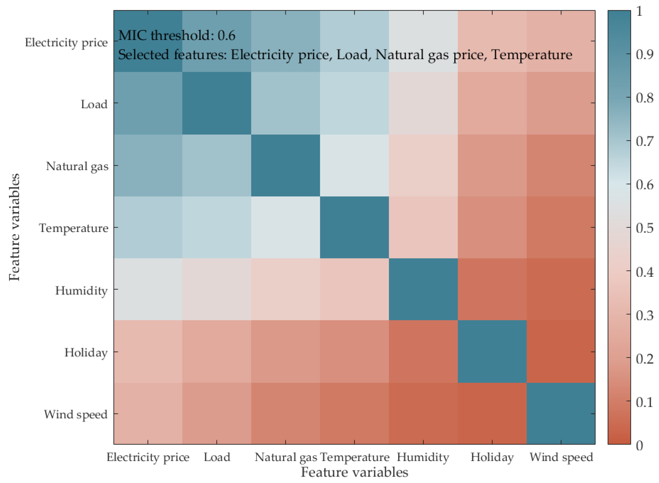
2.1. Feature Selection Approach Relying on the MIC

In the field of the electricity market, the accuracy of short-term electricity price prediction mainly depends on the reasonable choice of input characteristics. Given that day-ahead electricity prices are influenced by diverse factors, including historical electricity prices and loads, if all potentially influential factors are employed as input variables, it will bring in an excessive amount of noise and elevate the time and storage complexity of the model. Consequently, it becomes imperative to execute multidimensional correlation analytics targeting price-determinant variables within electricity markets, coupled with the implementation of systematic filtration protocols to isolate principal determinants impacting pricing mechanisms.
Common methods for correlation analysis include the Pearson correlation coefficient, Spearman’s rank correlation coefficient, and K-nearest neighbor distance. Compared to these methods, the maximum information coefficient based on mutual information theory has a broader applicability in measuring the correlation between two variables, lower computational complexity, and higher robustness [35]. MIC is often used as a feature selection method in machine learning and has the characteristics of non-parametricity, adaptability, scale invariance, and consistency. In the electricity markets of diverse regions, the characteristics of electricity price fluctuations and the influencing factors are distinct. MIC is capable of efficiently gauging the linear or nonlinear associations among variables. It offers a potent instrument for filtering out the sequences that exert a more substantial influence on electricity prices.
MIC gauges the correlation magnitude among variables via computing mutual information and implementing the grid division approach. The expression of mutual information (MI) is as follows:
k MI ( A , B ) = a A b B p ( a , b ) log p ( a , b ) p ( a ) p ( b )
where k MI ( A , B ) is mutual information. A = a i , i = 1 , 2 , , n and B = b i , i = 1 , 2 , , n stand for the joint probability density of variables A and B. p ( a , b ) and p ( b ) are used to represent the marginal probability densities of A and B, respectively. Consider D = a i , b i , i = 1 , 2 , , n , which is the set composed of the joint ordered pairs of A and B. A partitioning rule G is formulated. This rule serves to separately partition the value ranges of A and B into x and y segments. In other words, it divides them into a grid structure with x × y elements. The mutual information k MI ( A , B ) within each of the obtained grid partitions is calculated. The maximum value of k MI ( A , B ) among the partitioning methods is the maximum mutual information, and its expression is as follows:
k MI * ( D , x , y ) = max k MI ( D | G )
where D | G is the partition of data D under the rule G.
On this basis, the maximum normalized k MI ( A , B ) value under different division rules is obtained, and then a characteristic matrix is formed, and its expression is as follows:
M ( D ) x , y = k MI * ( D , x , y ) log min { x , y }
Then the expression of the maximum mutual information coefficient is as follows:
k MIC ( D ) = max x × y < B ( n ) M ( D ) x , y
where B ( n ) represents the upper bound value of the size of the grid partitioning, which is denoted as x × y . In this paper, B ( n ) = n 0.6 .
According to the above theory, the larger the value of k MIC ( D ) is, the stronger the correlation between variables is. When k MIC   ( D ) = 0 , the variables are independent of each other.

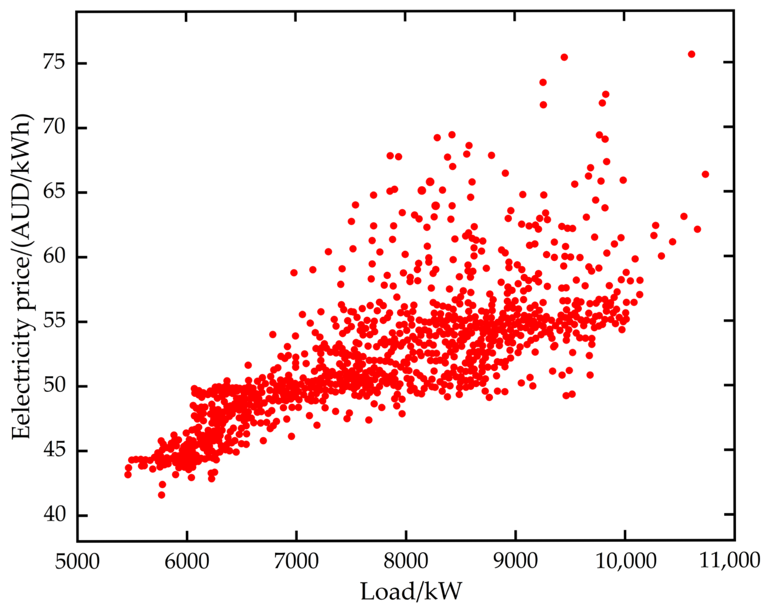
2.2. Analysis of the Nonlinear Characteristics of Electricity Price Data

First, the characteristics of the electricity pricing datasets themselves are analyzed. Electricity prices have complex characteristics such as seasonality, mean reversion, price–load correlation, volatility, high frequency, nonlinearity, extreme prices, and calendar effects. As depicted in Figure 1, which presents the daily electricity prices in different months in Australia, in terms of seasonality, the prices in summer are higher than those in other seasons, and the prices change with the hours. Owing to the low load demand, the electricity prices are at their lowest in the early morning hours. Conversely, they reach their peak during the morning and evening periods. There are also different price peaks in the afternoon and evening. There is an obvious correlation between the load and the price, and the price decreases as the load decreases.
In terms of extreme prices, as shown in Figure 2, the electricity prices in summer in Australia can reach five times the average level and then drop rapidly. Extreme prices occur more frequently in winter, while the prices in spring and autumn are relatively stable. Price spikes are influenced not only by the average price level but also by seasonal patterns such as daily, weekly, and seasonal ones. For example, a negative price peak may occur at 0:30 at night, which is mainly caused by the temporary market surplus resulting from the supply of intermittent renewable electricity (wind power). Once the problem is solved, the price will quickly return to normal.
The non-storability of electricity and various influencing factors, such as extreme loads caused by severe weather, unexpected events, power outages, transmission failures, etc., can all trigger price spikes. Figure 3 shows that the characteristics of price spikes change significantly within a day. A negative price peak occurs at 0:30 at night, which is mainly caused by the temporary market surplus resulting from the supply of intermittent renewable electricity. Once the problem is solved, the price will quickly return to normal. The negative peak reflects a distribution characteristic of the spot price. In addition, price peaks are influenced not only by the average price level but also by seasonal patterns such as daily, weekly, and seasonal ones.
In addition, the fluctuations of electricity spot prices exhibit a high degree of variability and possess a clustering characteristic. As depicted in Figure 4, the electricity prices in the Singapore electricity market exhibit obvious differences between weekdays and weekends. Due to the work factor in the morning on weekdays, the electricity prices are higher than those on weekend mornings. The price fluctuations on weekends are moderate and the range is relatively uniform, while there are more fluctuations and inconsistent ranges on weekdays. The price changes during holidays are different from those on weekdays and weekends.
Figure 5 is a scatter plot of the correlation between electricity prices and loads in New South Wales, Australia, in March 2013. From Figure 5, we can observe that when the load increases, the price also rises, indicating a strong correlation between the load and electricity prices in this market. However, it is extremely difficult to apply these factors to electricity price prediction in reality. On the one hand, it is very hard to collect all the data on these factors. Secondly, if these factors are used as input data, the computational efficiency of currently popular models will also decrease. Especially for methods like the artificial neural network (ANN), it will increase the dimensionality, resulting in excessive training, and the prediction results may not necessarily be good.
Although the behaviors and characteristics of electricity prices vary among different regions and countries, they all change over time. From an economic perspective, electricity prices can be regarded as different commodities. Moreover, since electricity prices are influenced by numerous factors, theoretically, taking all factors into account for electricity price prediction would lead to more accurate results. However, in practice, there are issues such as difficulties in data collection and a decrease in the computational efficiency of models. Therefore, selecting appropriate factors is crucial for improving the prediction accuracy of electricity prices.

2.3. Sorting of Multivariate Nonlinear Correlations and Screening of Key Factors

Upon ascertaining the approach for analyzing the correlation of electricity prices, a comprehensive analysis is carried out on the Singapore electricity market data in 2023 that has been amassed. This dataset is sampled once every 0.5 h and mainly includes information such as electricity prices, power loads, natural gas prices, holidays, temperatures, humidity levels, and wind speeds. The MIC approach is employed to compute the respective average MIC values of the electricity prices during this month in relation to power loads, natural gas prices, holidays, temperatures, humidity magnitudes, and wind velocities. The computed outcomes are presented in Figure 6, which visualizes the MIC matrix as a heatmap to enhance interpretability. The radar chart is shown in Figure 7. The nonlinear correlations between each feature and the electricity prices are evaluated through MIC, and then the key influencing factors are screened out.
From the calculation results, it can be known that the correlations between the features and the target variable are ranked from high to low as follows: international natural gas price, power load, temperature, humidity, holidays, and wind speed. Among them, the MIC values of electricity prices with natural gas, power load, and temperature are greater than 0.6, indicating that they have a strong correlation; while the MIC values of electricity prices with humidity, holidays, and wind speed are less than 0.6, showing a weak correlation. In particular, among the climate data, the correlation between temperature and electricity price is relatively high. This is because the hot climate in Singapore leads to a large demand for air-conditioning electricity. As the temperature rises, the power load will increase, thereby driving up the electricity price. Fundamentally, it is due to the fact that there exists a robust correlation between temperature and load. In light of the outcomes of the MIC correlation analysis, the international natural gas price, electrical load, and temperature are chosen as components of the feature inputs for the electricity price prediction model. Simultaneously, taking into account the periodic variation characteristics of electricity prices, the historical electricity price data are likewise utilized as a feature input for the model. Despite its excellent performance in static feature selection, MIC fails to capture the dynamic temporal associations between electricity prices and influencing factors. The impact of natural gas prices on electricity prices may significantly increase during energy crises. Future research could combine sliding window MIC or dynamic Bayesian networks to achieve adaptive updates of feature weights, thereby enhancing the model’s adaptability to market dynamics.

3. Theoretical Basis and Improvement of Multi-Objective Optimization Method

3.1. Theoretical Foundation of RBF

The RBF falls into the classification of feedforward neural networks. By making use of the radial basis function as its activation function, it has a strong ability for nonlinear mapping. The RBF neural network fundamentally features a tripartite architectural configuration comprising input, hidden, and output computational strata. Functionally, the input stratum serves as the primary interface for assimilating exogenous input vectors, which are subsequently propagated through nonlinear transformations to the kernel-processing hidden stratum.
The hidden layer is made up of a great quantity of neurons. And for every neuron within the hidden layer, the RBF is utilized as the activation mechanism. The centers and widths of these functions decide the response features of the neurons to the input signals. The output stratum synthesizes hidden stratum signals through weighted aggregation mechanisms, generating the network’s terminal computational results. Transformations between input and hidden spaces manifest nonlinear transformations, whereas hidden-to-output spatial mappings demonstrate linear algebraic operations.
Properly choosing the centers from the dataset represents the core of the RBF network. An optimal RBF network demands attaining the most favorable performance from the data. This condition can be fulfilled by judiciously selecting the centers via the utilization of a multi-objective algorithm.

3.2. Limitations of Standard NSGA-II

The NSGA-II was put forward by scholars Srinivas and Deb [36], and it represents an enhanced iteration of the NSGA algorithm. The predecessor of the NSGA algorithm is the well-known genetic algorithm. It incorporates a rapid non-dominated sorting operation on the foundation of the genetic algorithm, while the remaining operations are in accordance with those of the genetic algorithm. With the widespread application of the non-dominated genetic algorithm, the deficiencies of the NSGA algorithm have gradually emerged. First, the complexity of the algorithm known as NSGA is roughly of the order O m N 3 , which is relatively high. Second, the NSGA algorithm lacks an elitist selection strategy, resulting in the loss of many excellent individuals. Third, the setting of the radius parameter in the NSGA algorithm lacks objectivity. In order to address the abovementioned deficiencies, scholars carried out improvements, which led to the emergence of the NSGA-II algorithm. The primary distinctions between the NSGA-II and the NSGA are presented as follows: Firstly, it implements a rapid non-dominated sorting strategy, decreasing the computational complexity from O m N 3 to O m N 2 . This substantial reduction notably enhances the operational efficiency of the algorithm. Second, it introduces a crowding distance calculation method to improve population diversity and adopts an elitist selection strategy, which expands the sampling space to a certain extent.
However, the NSGA-II algorithm has some problems. Its fixed crowding distance-based individual sorting method lacks objectivity and completeness. This shortcoming will result in a decrease in the diversity of the solution ensemble and the algorithm’s optimization prowess. The elitist selection strategy will, to a certain degree, attenuate the convergence of the algorithm. There are also defects in the crossover and mutation operations, which are specifically as follows:
  • When the basic NSGA-II algorithm selects excellent population individuals, it places its dependence on two factors: the Pareto rank and the crowding distance. As the number of iterative steps grows, in the situation where the Pareto ranks of individuals are identical, the degree of crowding takes precedence in the process of individual selection. This algorithm uses a fixed crowding distance-based individual sorting method, which cannot scientifically reflect the distribution of the solution set. When a group of individuals with low crowding distances appears, eliminating such individuals may lead to the elimination of most individuals and change the crowding distances of other individuals. However, the fixed crowding distance sorting method ignores this dynamic change.
  • The elitist selection tactic of the fundamental NSGA-II algorithm integrates the non-dominated sorting of both the parent and offspring populations. It engages in competition to produce the subsequent generation and preserves some parent individuals, in part, to enhance the diversity of the population. However, it has obvious defects. It is easy to make the algorithm converge prematurely to a local optimal solution, and it also leads to a decrease in the overall convergence performance.
  • The fundamental NSGA-II algorithm assigns fixed values to the genetic operator probabilities. Typically, the crossover probability lies within the range of [0.9, 0.97], while the mutation probability ranges from [0.0001, 0.1]. These values exert a substantial influence on the solution outcome and the convergence of the algorithm. If the crossover probability is too high, it is easy to destroy the population pattern and the structure of excellent individuals in the algorithm. If it is too low, the search for the optimal solution will slow down or even stagnate. Should the mutation probability be exceedingly low, the generation of novel individuals becomes arduous, thereby diminishing the diversity of the population. If the value is overly large, the algorithm will degenerate into a random search. For diverse optimization problems, a substantial number of experiments are necessary to ascertain the crossover and mutation probabilities. Generally speaking, it is quite challenging to identify the optimal values. Therefore, the fixed crossover and mutation probabilities are obvious defects of this algorithm, which may easily lead to the degradation of the algorithm.

3.3. Proposed Improvements and Mechanisms

In an effort to surmount the inadequacies of conventional multi-objective optimization algorithms regarding the diversity of the solution set, the retention of elitism, and the prevention of premature convergence, this article undertakes optimizations at various levels. To address the issue of poor solution set diversity stemming from traditional crowding distance sorting, an improved strategy for calculating the crowding distance is presented. To prevent the algorithm from converging prematurely, while retaining excellent elite individuals and enhancing population diversity, the traditional elitist retention selection strategy is improved. To guarantee the diversity of the population individuals, the distribution of Pareto-optimal solutions is optimized, the premature convergence of the algorithm is avoided, a strategy for adaptively regulating crossover and mutation probabilities is implemented, and a local search operation is also incorporated. The specific details are as follows:
  • Improvement of the crowding distance calculation
The traditional fixed sorting method is abandoned. The relative crowding distance of different individuals is calculated using the Euclidean distance, and then the absolute distance is calculated based on it as the individual’s crowding distance to represent its degree of crowding. At the same time, the dominance of the solution is measured in combination with the initial fitness. The crowding distance of every individual is calculated in a comprehensive manner. Specifically, the crowding distances associated with the maximum and minimum fitness values are designated as infinity. The overall crowding distance is equivalent to the aggregation of the crowding distances of every individual. The improved crowding distance calculation, combined with the previously solved Pareto front, can more efficiently find the offspring population with high fitness and high individual richness, accelerating the optimization process of the algorithm. During optimization, individuals with large crowding distances are selected. Since the similarity between these individuals is low, it is beneficial to ensure the diversity of population individuals. Compared with the method of setting sharing parameters, it is less likely to fall into local optima.
For an individual k in the situation of a multi-objective optimization problem, assume that the set of multi-objective optimization functions contains S objective functions. The coordinates of individual K in the objective space are f 1 k , f 2 k , , f S k . For any two individuals k and k , the Euclidean distance formula between them in the objective space is:
d k k = s = 1 S f s , k f s , k 2
Assume that there are K k individuals in the neighborhood of individual k , and the relative crowding distance between individual k and an individual k in its neighborhood is D k . Then the formula for calculating the crowding distance of individual k is as follows:
D k = k = 1 , k k K k d k k a = 1 K b = 1 , b a K d a b
where D k represents the crowding distance of individual k . D k also denotes the relative crowding distance between individual k and an individual k within its neighborhood. K k is the quantity of individuals in the neighborhood of individual k . d a b is the relative crowding distance between the a -th and b -th individuals. K stands for the total number of individuals. f s , k is the value of the s -th objective function for individual k , f s , k is the value of the s -th objective function for individual k , and S represents the total number of objective functions.
The above-mentioned formula for calculating the crowding distance determines the degree of crowding of an individual in a local area by comparing the distance relationship between the individual and its surrounding individuals.
2.
Improved elitist retention strategy
In the traditional elitist retention strategy, the portion having a lower non-dominated level is preferentially chosen. Once the number of population individuals meets the standard, individuals with a higher non-dominated level cannot enter the new population. At this time, the crowding distance only affects the last selected non-dominated level, resulting in a lack of diversity in the population. In the improved elitist retention strategy proposed in this paper, the number of individuals to be deleted from each non-dominated level is first determined so that individuals from each non-dominated level have the opportunity to enter the new parent population. Furthermore, the lower the non-dominated level, the smaller the ratio of the individuals to be deleted, and the greater the number of individuals that are retained. This can not only retain the elite solutions but also increase the population diversity.
The formula for the number of individuals to be discarded from each non-dominated level is as follows:
Q g = g Q e 1 + 2 + + G 1 g G 1 Q e g = 1 G 1 Q g g = G
where Q g is the number of individuals to be discarded from non-dominated level g , Q e represents the quantity of individuals within the current population that surpass the number of individuals in the parent population, G is the number of non-dominated levels, ⌈ ⌉ is the ceiling function symbol, and Q g is the number of individuals to be discarded from non-dominated level g .
3.
Improved strategy for adaptive crossover and mutation probabilities
The larger the crossover probability, the greater the probability of changing the structure of existing individuals. However, if the original individual is relatively good, it may destroy the feasible solution. When the crossover probability is small, the algorithm is likely to fall into a local optimum. Therefore, the crossover probability of better individuals can be set to be smaller, and that of worse individuals can be set to be larger. A mutation can change the values of one or more genes in an individual. The execution of the mutation operation depends on the setting of the mutation probability, and the mutation probability is also adaptively adjusted.
The formula for calculating the crossover probability is as follows:
P k , c = P c 1 P c 1 P c 2 f avg f k f max f avg f k > f avg P c 1 f k f avg
where P k , c is the crossover probability of individual k , P c P c 2 , P c 1 , P c 2 and P c 1 denote the minimum and maximum values of the crossover probability, having values of 0.9 and 0.5, respectively. The fitness value of individual k is represented by f k , and f k is the maximum fitness value of all the individuals that are derived from performing the crossover operation of individual k with each individual within the target population, excluding individual k itself. f max and f avg are the maximum and average fitness values of all individuals in the target population, respectively.
The equation for calculating the mutation probability is as follows:
P k , m = P m 1 P m 1 P m 2 f avg f k f max f avg f k > f avg P m 1 f k f avg
where P k , m is the mutation probability of individual k , P k , m and P m 2 are the maximum and minimum values of the mutation probability, with values of 0.005 and 0.100, respectively, and f k is the fitness value of the individual obtained by mutating individual.
4.
Introduction of local search operation
After integrating the parent population and the offspring population to form a merged population, a local search operation is launched around the target individuals in this merged population. Subsequently, the searched individuals are contrasted with the target individuals. Those individuals demonstrating superior performance are preserved to seek more optimal solutions and guarantee the uniform distribution and comprehensiveness of the solutions. Among them, the target individuals include the individuals with a non-dominated sorting rank of 1 in the population of the previous parameter optimization iteration and the top 5 individuals in terms of crowding distance, excluding this individual.

4. The Day-Ahead Electricity Price Prediction Model Based on RBF and the Improved NSGA-II

4.1. The Design of Optimizing the Structure of the RBF Network with the NSGA-II

In the training process of the RBF, the key lies in determining several parameters, namely, the centers of the activation functions in the hidden layer, the spreading factors, and inter-stratum connection weights mediating hidden-to-output signal transduction. When these parameters are ascertained through conventional methods, issues like the challenge of precisely determining the number of nodes in the hidden layer will arise. Such a situation will have an impact on the performance of the network.
The improved NSGA-II is an effective multi-objective optimization algorithm that can find a balanced solution among multiple conflicting objectives and can be utilized to optimize the architecture of the RBF. The following will elaborate on the optimization process of the NSGA-II algorithm based on the form and structure of how the improved NSGA-II algorithm optimizes the RBF neural network structure in this paper.

4.1.1. Optimization Design of RBF Neural Network Structure

In the input layer, four factors, such as international natural gas price, power load, temperature, and historical electricity price, are selected as input variables, and the number of nodes in the input layer is set to 4.
The hidden layer serves as the vital component of the RBF neural network for realizing nonlinear mapping, and the determination of the number of its nodes is a significant step. At the beginning, it can be roughly set based on empirical formulas or simple experiments and, subsequently, optimized through the NSGA-II algorithm. The neurons within the hidden layer adopt the Gaussian radial basis function as the activation function, and its mathematical expression is presented as follows:
φ f ( x ) = exp x c f 2 2 σ f 2
where φ f ( x ) denotes the output of the f-th hidden-layer neuron, x is the input vector, c f is the center vector of the c f -th Gaussian radial basis function, which has the same dimension as the input vector x. σ f is the width parameter of the f-th radial basis function, and represents the Euclidean norm of the vector. This function computes the distance between the input vector x and the center vector c f and modifies it according to the width parameter σ f . Subsequently, it outputs the corresponding function value, thereby achieving the nonlinear transformation of the input data.
The parameter settings of the output stratum are calibrated based on the dimensionality characteristics of target variables requiring prediction. Given this study’s focus on 24-hour-ahead electricity price forecasting, a singular nodal configuration is implemented in the output layer. The output of the neurons in the output layer represents a linear combination of the outputs obtained from the hidden layer, and its calculation formula is given as follows:
y ^ n = f = 1 F w f φ f ( x )
where y ^ n represents the output of the output layer, F is the number of hidden-layer nodes, w f is the weight coefficient connecting the f-th hidden-layer node and the output-layer node. Through this coefficient, the nonlinear outputs of the hidden layer are linearly weighted and combined to obtain the final predicted output value.

4.1.2. Optimal Parameter Configuration

K-means clustering is used to initialize the number of hidden layer nodes F and the center of the radial basis function of RBF to accelerate the global search efficiency of improved NSGA-II. Improved NSGA-II further optimizes the hidden layer parameters to ensure the balance between the model complexity and accuracy. First, in the structural design of the RBF model, the K-means clustering algorithm is employed to classify the data. The number of neurons F in the hidden layer is equal to the number of categories of the classified data. The K-means algorithm can be used to obtain the clustering centers c f and the widths σ f of the radial basis functions, and c f represents the coordinate of the center point of the f′-th node in the network.
σ f = min f c f c f
The quality of the number of types in the data classification process will directly affect the performance of the RBF model. The NSGA-II algorithm is used to obtain the optimal value of F, that is, the optimal number of types.
For the initial setting of the connection weights w f , the initial values are usually randomly generated within a certain reasonable range. The initial values can be assigned to each w f by a random number generator within the interval [−1, 1]. This way, in the subsequent training and optimization process, the optimal weight configuration can be gradually found based on different initial weight states, and the negative gradient descent method is used to update the weights.
The error function and performance function of the RBF neural network are defined as follows:
e m , i = y i y ^ m , i
J m = 1 2 e m , i 2
The weight adjustment strategy of the output layer of the RBF is:
W m + 1 = W m η J m W
where W m + 1 denote the weight matrix corresponding to the (m + 1)-th round of iterative training. Meanwhile, W m + 1 stands for the weight matrix of the m-th iterative training. The term J m W signifies the gradient of the weight matrix during the m-th iterative training process. η represents the learning rate, with its value satisfying the condition 0 < η < 1. J m is defined as the performance function of the RBF neural network model in the m-th iterative training. e m , i represents the prediction error of the i-th sample within the training set when using the RBF neural network model during the m-th iterative training. y i refers to the day-ahead electricity price label value of the i-th sample in the training set. And J m W represents the predicted day-ahead electricity price value of the i-th sample in the training set, which is obtained through the prediction of the RBF neural network model in the m-th iterative training.
In view of the sensitivity to improved NSGA-II superparameters, we conducted a robustness analysis, and the results showed that when the crossover probability was 0.5–0.9 and the mutation probability was 0.005–0.1, the model had strong robustness to parameter fluctuations. The different parameters used by the improved NSGA-II algorithm in the simulation experiments of this paper are shown in Table 2.

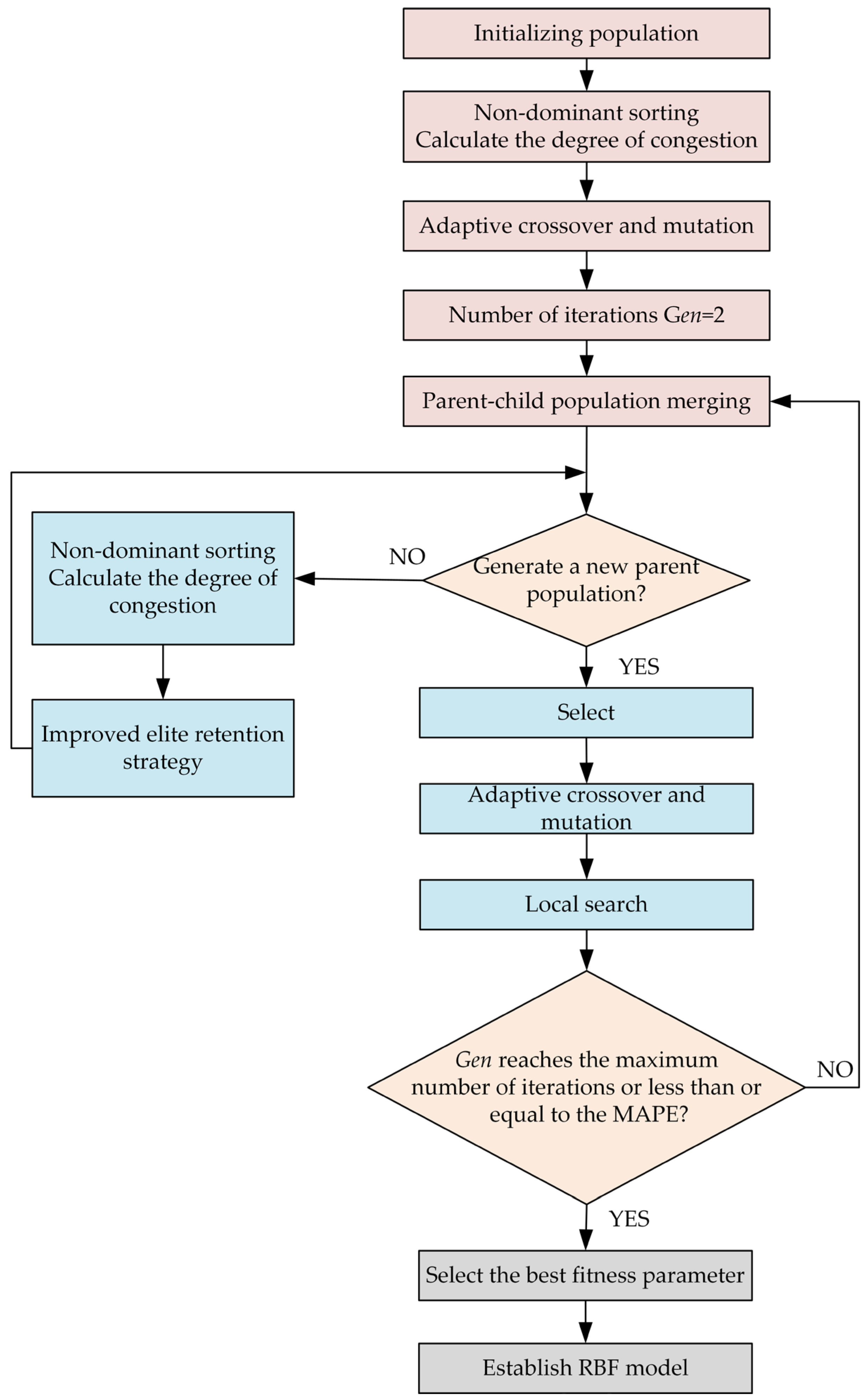
4.1.3. Multi-Objective Optimization Process

The procedure of optimizing the RBF network structure using the improved NSGA-II algorithm is depicted in Figure 8. The detailed optimization steps are as follows:
Step 1: Initialize the value of the parameter optimization iteration number t to 0.
Step 2: Take the initial parameters of the RBF neural network model as the individuals of the NSGA-II algorithm, initialize the population, and use the initialized population as the population for the t-th parameter optimization iteration.
Step 3: Employ the individuals within the population of the t-th parameter optimization iteration to establish the initial parameters of the RBF model and acquire the RBF neural network model corresponding to each individual.
Step 4: Use the training set to train the RBF model corresponding to each individual, respectively, and obtain the trained RBF model corresponding to each individual.
Step 5: Apply the test set to conduct tests on the trained RBF model corresponding to each individual and acquire the objective function value of the prediction accuracy for each individual, which serves as the fitness value of each individual.
Step 6: Based on the fitness value of each individual, perform non-dominated sorting on all the individuals within the population during the t-th iteration of the parameter optimization process. Subsequently, compute the crowding distance of each individual in the population during the t-th iteration of the parameter optimization procedure.
Step 7: Calculate the number of individuals to be discarded in each non-dominated level.
Step 8: Eliminate individuals within each non-dominated level in accordance with the quantity of individuals to be eliminated in each non-dominated level and the crowding distance of each individual, thereby acquiring the parent population.
Step 9: The evolutionary algorithm executes stochastic genetic operators (selection, genetic recombination, and stochastic variation) on parental candidate solutions, thereby propagating genetically optimized descendant populations through iterative evolutionary cycles.
Step 10: Combine the parent population and the offspring population so as to produce the population for the t + 1-th iteration of parameter optimization. Increment the value of t by 1, and then revert to the step of employing the individuals within the population of the t-th parameter optimization iteration to establish the initial parameters of the RBF model and acquire the RBF model corresponding to each individual. Carry out this procedure repeatedly until the maximum number of iterations is reached or some individuals meet the preset conditions. Output the trained RBF neural network model associated with the optimal individual as the final trained RBF neural network model. The preset conditions are as follows: an individual whose objective function of prediction accuracy is greater than the preset accuracy threshold and whose objective function of model complexity is less than the complexity threshold. The optimal individual refers to the one with the maximum objective function value of prediction accuracy. In cases where there are preset conditions, it is the individual among those meeting such conditions that has the largest objective function value of prediction accuracy.

4.1.4. Algorithm Pseudocode

In the following section, we present the pseudocode as described in Algorithm 1. This paper adopts clear step-by-step description and modular design to highlight the key steps of dynamic congestion calculation, adaptive parameter adjustment, and multi-objective optimization, which provides a clear program framework for implementing the proposed solution.
Algorithm 1: Improved NSGA-II-RBF Optimization
Input: training data Dtrain, test data Dtest, population size N, max iterations Tmax
Output: Pareto-optimal RBF models
 1 Initialize:
  Generate initial population P0 with RBF parameters (centers ci, widths σ i , weights wi) using K-means clustering.
  Set iteration t ← 0.
 2 While tTmax do:
 3 Fitness evaluation:
  For each individual iPt:
  Train RBF model Mi on Dtrain.
  Compute MAPE (Equation (16)) and complexity F (hidden nodes) using Dtest.
  Assign Fitnessi = (MAPEi, Fi).
 4 Non-dominated sorting:
  Rank individuals into Pareto fronts F 1 , F 2 ,… using fast non-dominated sorting.
 5 Dynamic crowding distance calculation:
  For each front F k :
   Compute pairwise Euclidean distances (Equation (5)).
   Update the crowding distance di using Equation (6) (incorporating local density and global distribution).
 6 Elite selection:
  Merge parent Pt and offspring Q t : R t = P t Q t .
  Select top N individuals from Rt by prioritizing:
   Lower Pareto rank.
   Higher dynamic crowding distance (to preserve diversity)
 7 Genetic operations:
  Adaptive crossover:
   For each pair (i,j):
    Compute crossover probability pc (Equation (8)) based on fitness.
    Perform simulated binary crossover if rand () < pc.
  Adaptive mutation:
   For each individual i:
    Compute mutation probability pm (Equation (9)).
    Apply polynomial mutation if rand() pm.
 8 Local search:
  For the top 5% elite individuals:
   Perturb parameters c i , σ i , w i within a neighborhood.
   Retain improved solutions to refine the Pareto front.
 9 tt + 1.
 10 Return Pareto-optimal RBF models from final population PTmax.

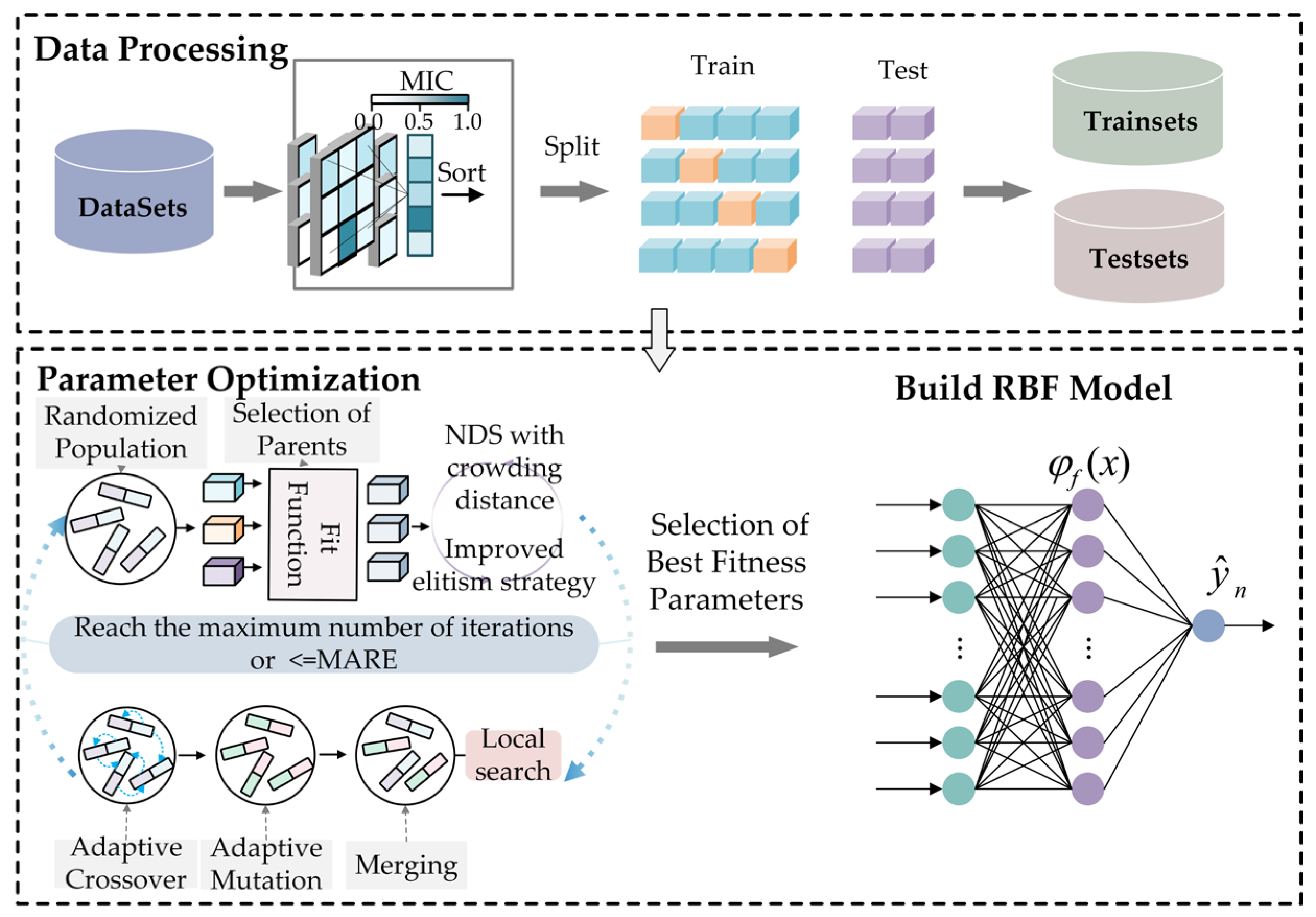
4.2. Prediction Model Framework and Implementation Steps

The flow of the day-ahead electricity price prediction model founded on the RBF and the enhanced NSGA-II, as put forward in this paper, is presented in Figure 9. The construction procedures are as follows.
  • Obtain historical electricity price data and data from multiple influencing factors, and use the MIC method to conduct a feature correlation analysis of the influencing factors.
  • Input the historical electricity price data and influencing factor data, and preprocess all the data.
  • Formulate a multi-objective optimization function. In this function, the objective function for prediction precision is the MAPE, and the objective function for model intricacy is the number of nodes within the hidden layer of the RBF neural network model. The calculation formula for the MAPE is as follows:
M A P E = 1 N n = 1 N y n y ^ n y n × 100 %
where MAPE represents the mean absolute percentage error. N denotes the quantity of samples in the test set. y n stands for the day-ahead electricity price label value of the n-th sample within the test set. y ^ n is the predicted day-ahead electricity price value of the n-th sample in the test set, and this predicted value is derived from the prediction made by the RBF neural network model.
During each iteration, the parameters of the RBF neural network associated with the population individuals are input into the network. Once the network has completed its training using the training dataset, the mean squared error between the predicted result and the actual value is calculated on the validation dataset. The objective of the algorithmic optimization is to reduce the MAPE value to its minimum. That is to say, the goal is to make the predicted value approach the actual value as closely as possible, thus improving the model’s prediction accuracy for short-term electricity price data.
In order to avoid constructing an overly complex RBF neural network model, the number of nodes, denoted as F, within the hidden layer of the RBF neural network model serves as an index for gauging the complexity of the model. The objective is to minimize the value of F under the condition of guaranteeing prediction precision. In other words, it aims to simplify the model, enhancing its generalization capacity and practical applicability. By doing so, while accurately forecasting short-term electricity prices, the model will not be overly intricate for application and maintenance purposes.
4.
Through feature extraction, use the NSGA-II algorithm to optimize the structure of the RBF neural network and train the model.
5.
Generate and present the prognoses regarding the day-ahead electricity price.

5. Comparative Analysis of Simulation Experiment and Model Performance

5.1. Dataset Construction and Preprocessing Method

5.1.1. Data Collection and Seasonal Division of Singapore Electricity Market

The electricity price curve has seasonal characteristics and usually has daily and weekly cycles. The training dataset is partitioned into weekday data spanning from Monday to Friday and weekend data corresponding to Saturday and Sunday. In the course of RBF neural network training, for each season, dates with resemblance must be chosen. For instance, to forecast the electricity price for a Monday or a Sunday, eight comparable days are picked for training. From among these similar days, one day is designated as the test data.
The measured data of the Singapore electricity market from 1 January 2023 to 31 December 2023 are selected as the dataset. This dataset includes electricity prices, international natural gas prices, power loads, and temperatures, with sampling carried out once every 0.5 h. In this study, the data sourced from the Singapore electricity market are utilized to train and test the proposed methodology. To enable a comparison, the RBF and other algorithms are also set up for the testing procedure. The dataset is partitioned into two components: the training data and the test data. The specific particulars are illustrated in Table 3. The training data are employed in the training procedure and, concurrently, for the update of the bias and the learning rate. Upon the completion of the training, the test data are utilized to validate the efficacy of the proposed method. In view of the data missing problem, the linear interpolation method is used to complete the continuous missing values, and non-continuous missing records caused by equipment failure are eliminated. For extreme outliers, winsorization tailing treatment is adopted to retain the price spike characteristics while avoiding model overfitting.

5.1.2. Data Normalization

To mitigate the negative impacts of data features with diverse magnitudes on the ensuing neural network training procedure, expedite the training velocity, and enhance the training outcome, normalizing the assorted types of data that have been amassed and purified becomes imperative. In this manuscript, the min-max normalization technique is utilized to map the values of each data feature to a predefined interval. The computational formula for the normalization process is as follows:
n ¯ = n n min n max n min
where n ¯ represents the normalized data, n denotes the original simulation data, n is the minimum value of the data, and n max is the maximum value of the data. Through the min-max normalization, the original data are linearly mapped to the [0, 1] interval to eliminate the influence of dimensional differences on model training.
After such a normalization operation, all input data are within the same magnitude range, which is convenient for the subsequent processing of the RBF neural network.

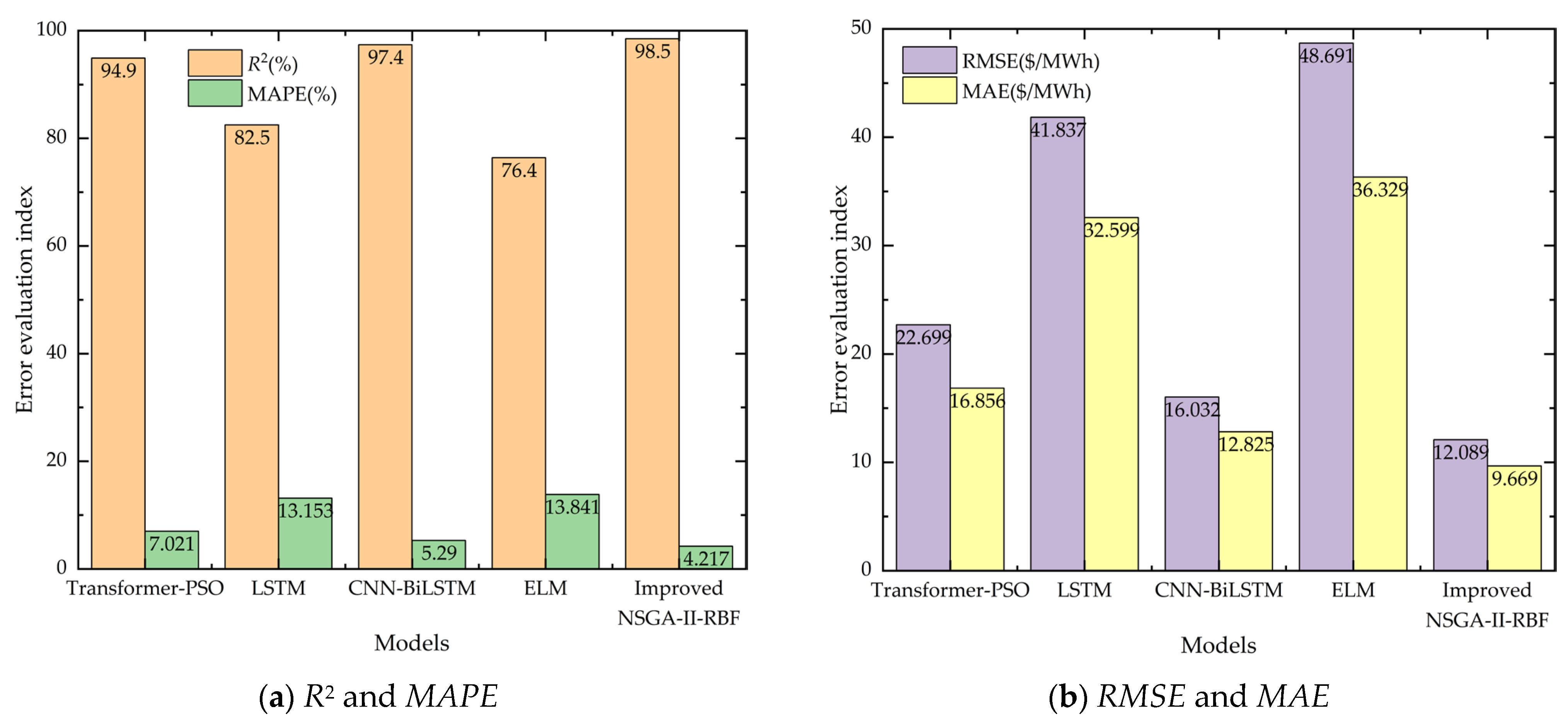
5.2. Error Evaluation Index

During the execution of error analysis, the chosen prediction performance metrics consist of four evaluation indices: MAE, RMSE, MAPE, and the coefficient of determination R2. Among them, the smaller the values of the MAE, RMSE, and MAPE, the higher the prediction accuracy. Conversely, R2 demonstrates stronger correspondence between forecasted and empirically observed electricity price trajectories, with heightened R2 magnitudes corresponding to enhanced congruency in their temporal fluctuation patterns. The calculation formulas are presented as follows:
X M A E = 1 N i = 1 N y ^ i y i
X R M S E = 1 N i = 1 N y ^ i y i 2
R 2 = 1 i = 1 N y ^ i y i 2 i = 1 N y i ¯ y i 2
where y i ^ is the predicted electricity price value at the i-th time point on the day to be measured, y i is the actual electricity price value at the i-th time point on the day to be measured, y i ¯ is the average value of the day-ahead electricity prices at all time points on the day to be measured, and N is the total number of prediction points.

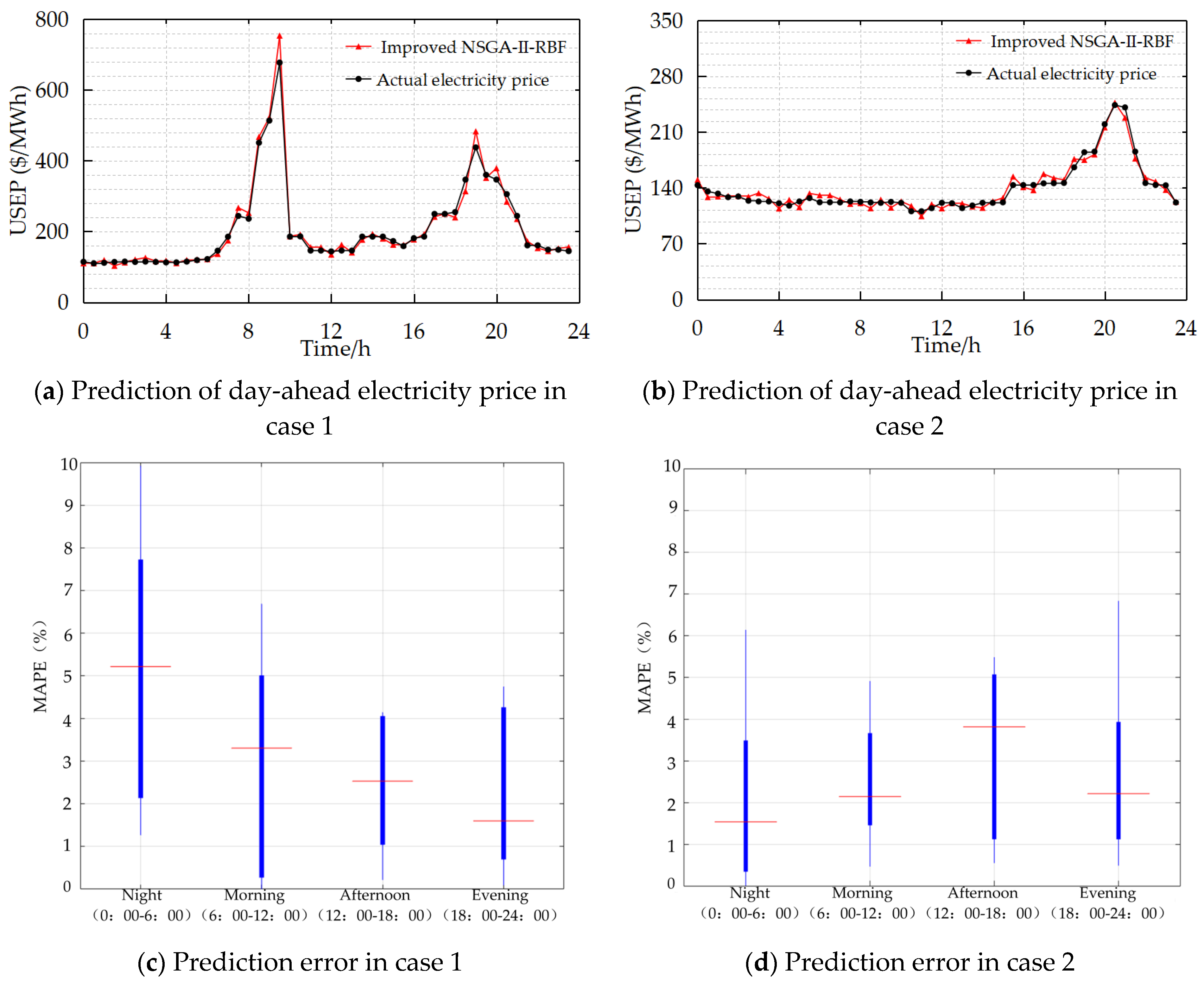
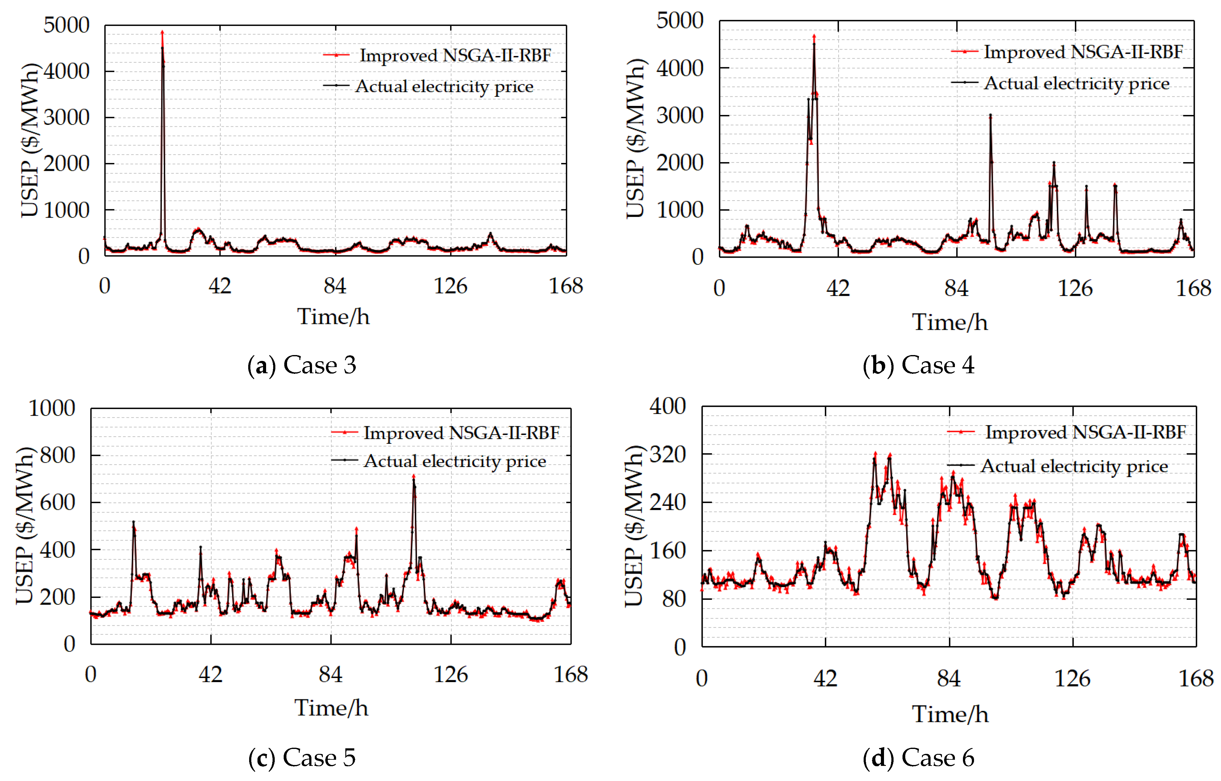
5.3. Analysis of Prediction Results and Algorithm Performance

To thoroughly evaluate the model’s predictive performance at different times, based on the actual electricity price data from Singapore’s power market on 23 July 2023, which was a low-volatility day, and 24 July 2023, which was a high-volatility day, error analysis was conducted for four time periods: night, morning peak, noon, and evening peak. Figure 10 shows the box-and-whisker plots of the day-ahead electricity price forecast results and MAPE for each time period in Case 1 and Case 2.
As shown in Figure 10a, the MAPE of the RBF amounts to 4.941%. The predicted peak prices during the morning rush hour closely matched the actual values, demonstrating the model’s effective capture. The rapid decline in afternoon prices deviated from expectations, with the actual price drop exceeding the forecast, possibly due to unquantified short-term market factors. However, the MAPE of the improved NSGA-II-RBF was only 4.941%, indicating its ability to track extreme volatility. Figure 10c shows that the median error is the smallest on the high-fluctuation day and night, and the median error outlier increases in the morning rush hour. The median error at noon is 5.04%, which is significantly higher than in other periods, and the median error in the evening rush hour is 6.79%, but the MAPE is still less than 7%, indicating that the model is still robust under extreme fluctuations.
Similarly, Figure 10b exhibits the day-ahead electricity price prediction scenario of Case 2. The forecast curve of the low-fluctuation scenario throughout the day is closely aligned with the actual value and only slightly underestimated in the afternoon. This is related to the reduction in the commercial load on weekends and the simplification of electricity price driving factors, and the model has strong generalization for the stable mode. The MAPE value of the method proposed in this paper is approximately 4.126%. From Figure 10d, it can be seen that the nighttime model has excellent stability during the low-fluctuation period, with a small increase in error during the morning rush hour and a slightly wider distribution of error during noon, which is related to the randomness of electricity price caused by photovoltaic output fluctuations. The median error during the evening rush hour is 5.26%, indicating that the model can still effectively track the peak of electricity price. The aforesaid outcomes signify that this method is capable of discerning a more optimal solution.
Figure 11 displays the weekly electricity price prediction outcomes of Case 3, Case 4, Case 5, and Case 6, respectively. Figure 11a typifies a standard spring week, and the electricity price predicted by the RBF is proximate to the actual value. As is evident from Figure 11b, the RBF has the capacity to trace the price increase that transpires within the 25th to 48th hours of this week. In this case, the MAPE of the RBF method is 4.481%.
Analogously, Figure 11c,d present the weekly electricity price prediction outcomes for Case 5 and Case 6, which, respectively, stand for a typical autumn week and a typical winter week. Regarding Case 5, the weekly MAPE value of the optimized RBF amounts to 4.931%, being the lowest among Cases 3 to 6. For Case 6, the MAPE of the optimized RBF is 5.013%, which is extremely close to the MAPE of Case 3. As observable from Figure 11c,d, the more significant the electricity price fluctuation, the larger the predicted MAPE value will be. The results show that the model prediction curve is highly consistent with the actual price trend and can effectively capture the seasonal load fluctuations, such as the price peak caused by high temperature in summer, short-term fluctuations caused by heating in winter, and the difference between weekdays and weekends in a week.

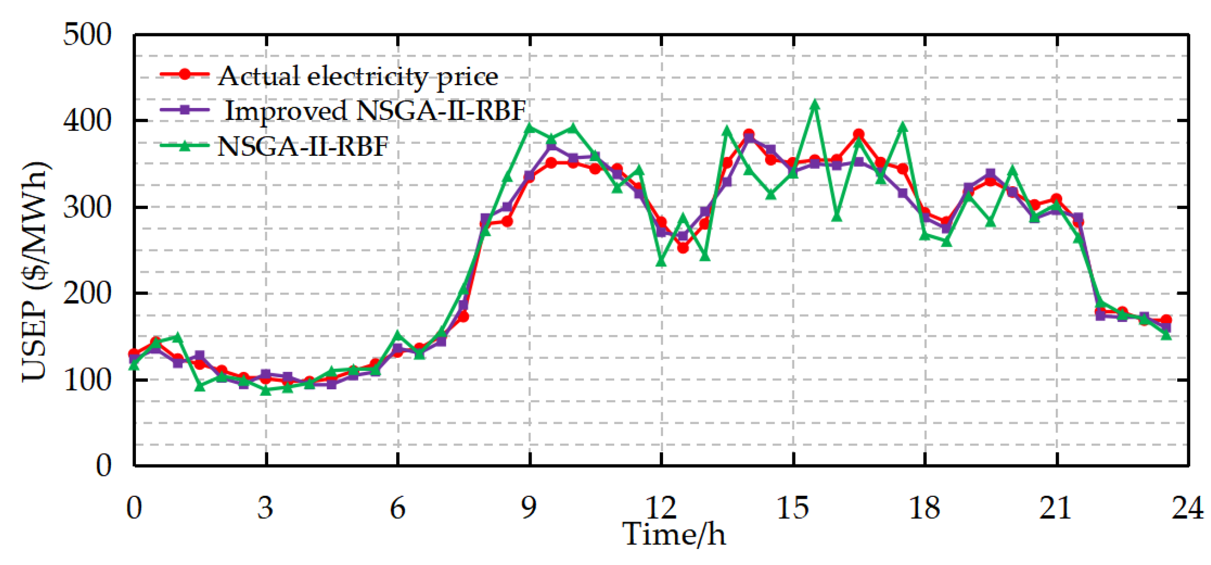
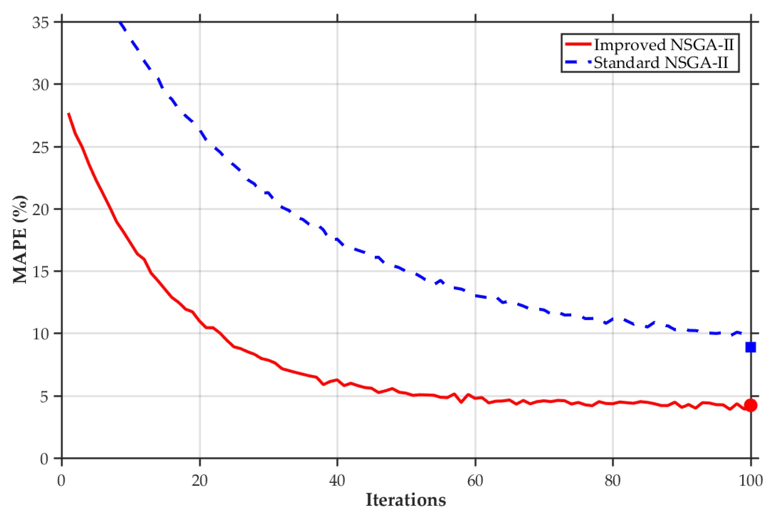
5.3.1. Analysis on the Comparison Between the Model Prior to and Subsequent to the Enhancement of NSGA-II

To illustrate the preeminence of the model presented in this paper, subsequent to enhancing the NSGA-II algorithm, a comparison is made with the model without the enhanced NSGA-II. The same dataset, which is based on the measurement data of the Singapore electricity market from June 1 to 29, is used to predict the day-ahead price of electricity on June 30. The final prediction result is obtained by using the average value obtained from multiple experiments in the test set. The experimental findings are depicted in Figure 12 and Table 4. In order to intuitively express the advantages of the improved algorithm, the convergence curves of standard NSGA-II and improved NSGA-II are shown in Figure 13.
As discernible from Figure 12, the predicted electricity price curve of the RBF model with the enhanced NSGA-II algorithm proposed herein is closer to the actual electricity price curve. In contrast, the accuracy of the prediction outcomes of the RBF model employing the unimproved NSGA-II algorithm is significantly lower compared to that of the model presented in this paper. From Figure 13, we know that the adaptive crossover in the improved algorithm dynamically adjusts crossover and mutation probabilities based on individual fitness, balancing global exploration with local development to prevent the algorithm from getting trapped in local optima. Local search performs fine-grained neighborhood searches for elite solutions, enhancing solution accuracy and diversity, ensuring a uniform distribution of the Pareto frontier. This improved hybrid strategy significantly accelerates convergence, reducing the number of iterations by 30%, and improves prediction accuracy.
As is evident from Table 4, the evaluation indices of the RBF model that utilizes the improved NSGA-II for day-ahead electricity price prediction are lower in value, which implies a superior prediction performance. When compared with the unoptimized RBF model, the MAE, RMSE, and MAPE of the model put forward in this paper have declined by 56.57%, 57.54%, and 52.41%, respectively. Meanwhile, the coefficient of determination R2 has increased by 7.2%. This clearly demonstrates that the enhancement of the NSGA-II algorithm has augmented the prediction accuracy of the model. The traditional NSGA-II-RBF model is unable to efficiently balance model complexity. Specifically, the quantity of nodes in the hidden layer is relatively large, a situation that might lead to problems of overfitting. The improved NSGA-II-RBF, through dynamic crowding degree calculation and adaptive parameter adjustment, significantly reduces the number of hidden layer nodes after optimization, reducing the complexity while ensuring the accuracy, based on the same hardware environment: Intel i7-12700H CPU, 32GB RAM, NVIDIA RTX 3070 GPU. The average runtime of a single iteration for the improved NSGA-II-RBF model and the traditional NSGA-II-RBF model was recorded. Experimental results show that the improved NSGA-II algorithm, through dynamic crowding distance calculation and adaptive parameter adjustment, significantly reduced the number of iterations required to converge, decreasing the single iteration time from 12.3 s in the traditional NSGA-II to 9.8 s.

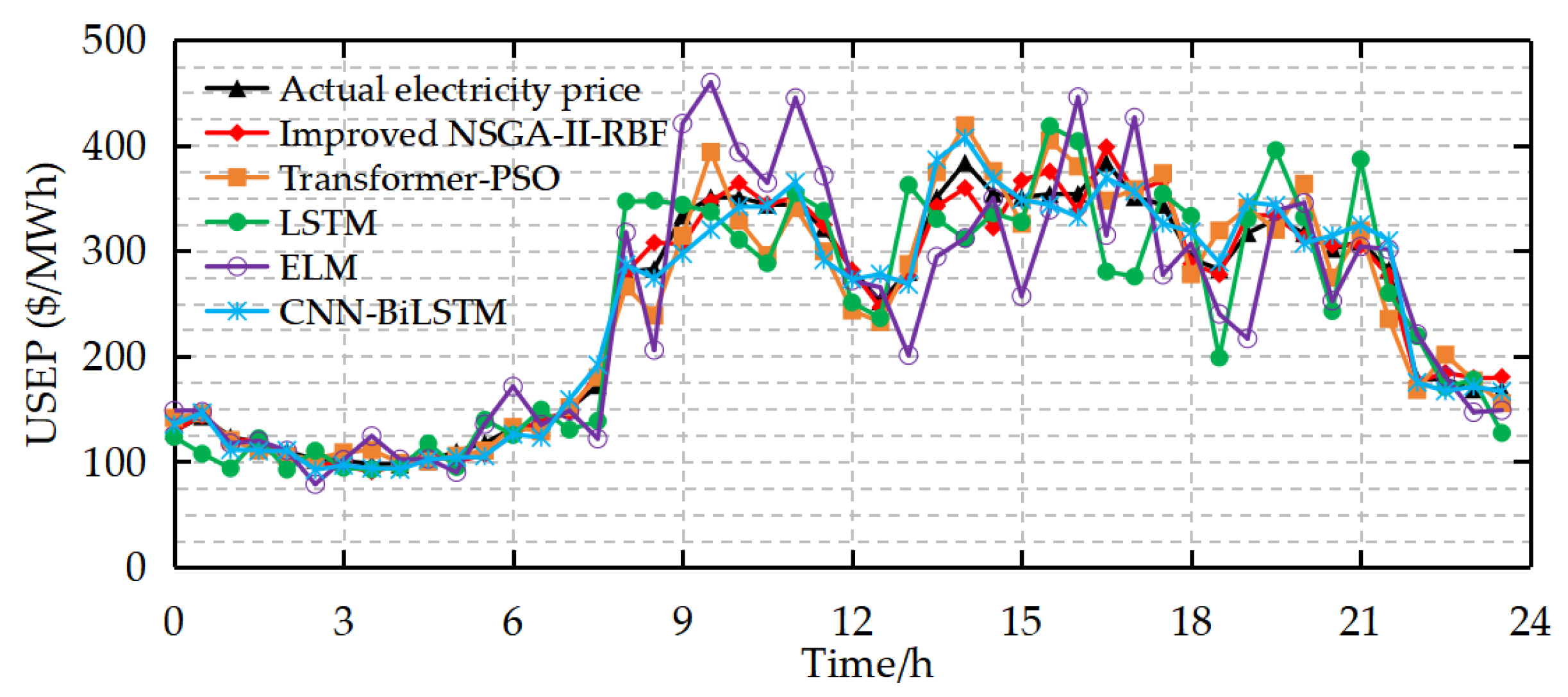
5.3.2. Comparative Analysis of Different Models

To further validate the preeminence of the model put forward in this paper, the model presented herein is contrasted with the LSTM, transformer-particle swarm optimization (Transformer-PSO), extreme learning machine (ELM), and convolutional neural network/bidirectional long short-term memory (CNN-BiLSTM) models. An identical dataset is employed as the input, and the final prediction outcomes are acquired by calculating the average value from multiple experiments. The experimental results are shown in Figure 14 and Figure 15, respectively.
As is evident from Figure 14, the predicted electricity price curve of the model presented in this paper shows a closer approximation to the actual electricity price curve. When contrasted with other models, it exhibits a more robust learning capacity regarding historical electricity prices and influencing factors. This provides additional validation for the accuracy of the model put forward in this paper.
As is observable from Figure 15, the evaluation indices of the model presented in this paper are all lower in value compared to those of the models used for comparison. As can be seen from Figure 15a,b, compared with the CNN-BiLSTM model, the improved NSGA-II-RBF reduces MAE, RMSE, and MAPE by 24.61%, 24.59%, and 20.28%, respectively, and increases R2 by 1.13%. This proves the advantages and accuracy of the model presented in this paper.
To quantify the statistical significance of performance differences between models, this paper employs paired t-tests to analyze prediction errors such as MAE, RMSE, and MAPE. The null hypothesis H0 is ‘there is no significant difference in model performance’, with a significance level set at α = 0.05. If the p-value < 0.05, the null hypothesis is rejected, indicating that there is a statistically significant difference between the models.
As shown in Table 5, in the comparison of improved NSGA-II-RBF with LSTM, Transformer-PSO, and other models, all p-values are below 0.05, indicating that the performance improvement is statistically significant. Compared to LSTM, the p-value for MAE is 0.003, rejecting the null hypothesis, confirming that the improved model significantly reduces prediction errors.

6. Conclusions

This research centers on the prediction of day-ahead electricity prices in sustainable power markets, and it aims to tackle the issue of price fluctuations that are brought about by the integration of renewable energy sources. A novel multi-objective optimization model combining improved NSGA-II and RBF neural networks is proposed. Through in-depth analysis of electricity price dynamics and feature selection using the MIC method, the model effectively captures nonlinear price characteristics while balancing prediction accuracy and computational complexity. Compared with multiple benchmark models, the proposed approach demonstrates superior prediction performance and robust adaptability to seasonal variations and price spikes. Key conclusions drawn from this research include the following:
  • The MIC-based feature selection method successfully identifies critical factors, such as international gas prices, electricity load, and temperature. By integrating these features with historical price data, the model optimizes input data quality and significantly improves prediction accuracy.
  • The improved NSGA-II algorithm outperforms traditional optimization methods in RBF network training. Through dynamic crowding degree calculation, adaptive crossover and mutation probabilities, and enhanced elitist retention strategies, it maintains population diversity, accelerates convergence, and avoids local optima to find optimal network parameters.
  • The proposed model overcomes limitations of conventional methods in handling nonlinearity, high-frequency dynamics, and multivariate dependencies. It provides a reliable prediction tool for sustainable market operations, enabling stakeholders to formulate optimal strategies, reduce renewable energy curtailment, and promote grid sustainability.
While this research has achieved significant advancements, several opportunities for improvement exist. Due to the completeness of public data in the Singapore market, this paper does not directly include wind and solar power output data. However, the model indirectly captures the impact of renewable energy fluctuations through international natural gas prices. Future research can integrate real-time renewable energy output indicators to further enhance the model’s adaptability to low-carbon electricity markets. The dynamic congestion calculation and adaptive parameter adjustment mechanism of this framework can adapt to the fluctuation characteristics of different markets. It can be applied to other markets in the future to reflect its better performance. Practical applications in market trading strategies and grid dispatch optimization should be investigated to strengthen real-world relevance and operational effectiveness, thereby supporting the stable development of sustainable power systems.

Author Contributions

Conceptualization, S.S. and D.W.; methodology, C.L.; software, Y.S.; validation, Y.S.; formal analysis, Z.L.; investigation, G.Z.; resources, G.Z.; data curation, Z.L.; writing—original draft preparation, C.L.; writing—review and editing, S.Q.; visualization, S.Q.; supervision, S.S.; project administration, D.W.; funding acquisition, D.W. All authors have read and agreed to the published version of the manuscript.

Funding

This research was funded by the National Natural Science Foundation of China (Grant No. 52407011).

Institutional Review Board Statement

Not applicable.

Informed Consent Statement

Not applicable.

Data Availability Statement

The raw data supporting the conclusions of this article will be made available by the authors on request.

Conflicts of Interest

Authors Zhenghan Liu and Guifan Zhang were employed by the company State Grid Jibei Electric Power Co., Ltd. The remaining authors declare that the research was conducted in the absence of any commercial or financial relationships that could be construed as a potential conflict of interest.

References

  1. Liu, J.; Wang, J.; Cardinal, J. Evolution and reform of UK electricity market. Renew. Sustain. Energy Rev. 2022, 161, 112317. [Google Scholar] [CrossRef]
  2. Hu, J.; Harmsen, R.; Crijns-Graus, W.; Worrell, E.; van den Broek, M. Identifying barriers to large-scale integration of variable renewable electricity into the electricity market: A literature review of market design. Renew. Sustain. Energy Rev. 2018, 81, 2181–2195. [Google Scholar] [CrossRef]
  3. Zhang, B.; Tian, H.; Berry, A.; Huang, H.; Roussac, A.C. Experimental comparison of two main paradigms for day-ahead average carbon intensity forecasting in power grids: A case study in Australia. Sustainability 2024, 16, 8580. [Google Scholar] [CrossRef]
  4. Ibebuchi, C.C. Day-Ahead Energy Price Forecasting with Machine Learning: Role of Endogenous Predictors. Forecasting 2025, 7, 18. [Google Scholar] [CrossRef]
  5. Lago, J.; Marcjasz, G.; De Schutter, B.; Weron, R. Forecasting day-ahead electricity prices: A review of state-of-the-art algorithms, best practices and an open-access benchmark. Appl. Energy 2021, 293, 116983. [Google Scholar] [CrossRef]
  6. Xu, H.; Ma, J.; Xue, F.; Li, X.; Li, H.; Wang, W.; Zhong, Y.; Zhao, J.; Zhang, Y. Optimization control strategy for photovoltaic/hydrogen system efficiency considering the startup process of alkaline electrolyzers. Int. J. Hydrogen Energy 2025, 106, 65–79. [Google Scholar] [CrossRef]
  7. Klyuev, R.V.; Morgoev, I.D.; Morgoeva, A.D.; Gavrina, O.A.; Martyushev, N.V.; Efremenkov, E.A.; Mengxu, Q. Methods of forecasting electric energy consumption: A literature review. Energies 2022, 15, 8919. [Google Scholar] [CrossRef]
  8. Karabiber, O.A.; Xydis, G. Electricity price forecasting in the Danish day-ahead market using the TBATS, ANN and ARIMA methods. Energies 2019, 12, 928. [Google Scholar] [CrossRef]
  9. Ioannidis, F.; Kosmidou, K.; Savva, C.; Theodossiou, P. Electricity pricing using a periodic GARCH model with conditional skewness and kurtosis components. Energy Econ. 2021, 95, 105110. [Google Scholar] [CrossRef]
  10. Gonzalez, J.P.; Roque, A.M.S.M.S.; Perez, E.A. Forecasting functional time series with a new Hilbertian ARMAX model: Application to electricity price forecasting. IEEE Trans. Power Syst. 2018, 33, 545–556. [Google Scholar] [CrossRef]
  11. Alsuwaylimi, A.A. Comparison of ARIMA, ANN and hybrid (ARIMA–ANN) models for time series forecasting. Inf. Sci. Lett. 2023, 12, 1003–1016. [Google Scholar]
  12. Blfgeh, A.; Alkhudhayr, H. A Machine Learning-Based Sustainable Energy Management of Wind Farms Using Bayesian Recurrent Neural Network. Sustainability 2024, 16, 8426. [Google Scholar] [CrossRef]
  13. Aksan, F.; Li, Y.; Suresh, V.; Janik, P. CNN-LSTM vs. LSTM-CNN to predict power flow direction: A case study of the high-voltage subnet of northeast Germany. Sensors 2023, 23, 901. [Google Scholar] [CrossRef] [PubMed]
  14. Xuan, H.; Maestrini, L.; Chen, F.; Grazian, C. Stochastic variational inference for GARCH models. Stat. Comput. 2024, 34, 45. [Google Scholar] [CrossRef]
  15. Keles, D.; Scelle, J.; Paraschiv, F.; Fichtner, W. Extended forecast methods for day-ahead electricity spot prices applying artificial neural networks. Appl. Energy 2016, 162, 218–230. [Google Scholar] [CrossRef]
  16. Abisoye, B.O.; Sun, Y.; Zenghui, W. Survey of Artificial Intelligence Methods for Renewable Energy Forecasting: Methodologies and Insights. Renew. Energy Focus 2024, 48, 100529. [Google Scholar] [CrossRef]
  17. Bian, K.; Priyadarshi, R. Machine Learning Optimization Techniques: A Survey, Classification, Challenges, and Future Re-search Issues. Arch. Comput. Methods Eng. 2024, 31, 4209–4233. [Google Scholar] [CrossRef]
  18. Loizidis, S.; Kyprianou, A.; Georghiou, G.E. Electricity market price forecasting using ELM and bootstrap analysis: A case study of the German and Finnish day-ahead markets. Appl. Energy 2024, 363, 123058. [Google Scholar] [CrossRef]
  19. Shejul, K.; Harikrishnan, R.; Gupta, H. The improved integrated exponential smoothing based CNN-LSTM algorithm to forecast the day-ahead electricity price. MethodsX 2024, 13, 102923. [Google Scholar] [CrossRef]
  20. Xiong, X.; Qing, G. A hybrid day-ahead electricity price forecasting framework based on time series. Energy 2023, 264, 126099. [Google Scholar] [CrossRef]
  21. Sridharan, V.; Tuo, M.; Li, X. Wholesale electricity price forecasting using integrated long-term recurrent convolutional network model. Energies 2022, 15, 7606. [Google Scholar] [CrossRef]
  22. Zhang, T.; Tang, Z.; Wu, J.; Du, X.; Chen, K. Short term electricity price forecasting using a new hybrid model based on two-layer decomposition technique and ensemble learning. Electr. Power Syst. Res. 2022, 205, 107762. [Google Scholar] [CrossRef]
  23. Jiang, P.; Nie, Y.; Wang, J.; Huang, X. Multivariable short-term electricity price forecasting using artificial intelligence and multi-input multi-output scheme. Energy Econ. 2023, 117, 106471. [Google Scholar] [CrossRef]
  24. Ghimire, S.; Deo, R.C.; Casillas-Pérez, D.; Salcedo-Sanz, S. Two-step deep learning framework with error compensation technique for short-term, half-hourly electricity price forecasting. Appl. Energy 2024, 353, 122059. [Google Scholar] [CrossRef]
  25. Sai, W.; Pan, Z.; Liu, S.; Jiao, Z.; Zhong, Z.; Miao, B.; Chan, S.H. Event-driven forecasting of wholesale electricity price and frequency regulation price using machine learning algorithms. Appl. Energy 2023, 352, 121989. [Google Scholar] [CrossRef]
  26. Fraunholz, C.; Kraft, E.; Keles, D.; Fichtner, W. Advanced price forecasting in agent-based electricity market simulation. Appl. Energy 2021, 290, 116688. [Google Scholar] [CrossRef]
  27. Laitsos, V.; Vontzos, G.; Bargiotas, D.; Daskalopulu, A.; Tsoukalas, L.H. Data-driven techniques for short-term electricity price forecasting through novel deep learning approaches with attention mechanisms. Energies 2024, 17, 1625. [Google Scholar] [CrossRef]
  28. Wu, H.; Liang, Y.; Heng, J.-N.; Ma, C.-X.; Gao, X.-Z. MSV-net: Multi-scale visual-inspired network for short-term electricity price forecasting. Energy 2024, 291, 130350. [Google Scholar] [CrossRef]
  29. Chen, H.; Zhang, J.; Zhang, C.; Qiao, N.; Zhang, J.; Li, Q. Research on short-term electricity price prediction in power market based on BP neural network. In Proceedings of the 2022 9th International Forum on Electrical Engineering and Automation (IFEEA), IEEE, Zhuhai, China, 4–6 November 2022; pp. 1198–1201. [Google Scholar]
  30. Bashir, T.; Haoyong, C.; Tahir, M.F.; Liqiang, Z. Short term electricity load forecasting using hybrid prophet-LSTM model optimized by BPNN. Energy Rep. 2022, 8, 1678–1686. [Google Scholar] [CrossRef]
  31. Hadjout, D.; Torres, J.; Troncoso, A.; Sebaa, A.; Martínez-Álvarez, F. Electricity consumption forecasting based on ensemble deep learning with application to the Algerian market. Energy 2022, 243, 123060. [Google Scholar] [CrossRef]
  32. Geng, G.; He, Y.; Zhang, J.; Qin, T.; Yang, B. Short-term power load forecasting based on PSO-optimized VMD-TCN-attention mechanism. Energies 2023, 16, 4616. [Google Scholar] [CrossRef]
  33. Jia, W.; Zhao, D.; Shen, T.; Su, C.; Hu, C.; Zhao, Y. A new optimized GA-RBF neural network algorithm. Comput. Intell. Neurosci. 2014, 2014, 982045. [Google Scholar] [CrossRef] [PubMed]
  34. Tao, J.; Yu, Z.; Zhang, R.; Gao, F. RBF neural network modeling approach using PCA based LM–GA optimization for coke furnace system. Appl. Soft Comput. 2021, 111, 107691. [Google Scholar] [CrossRef]
  35. Zhang, Y.; Shang, P. KM-MIC: An improved maximum information coefficient based on K-Medoids clustering. Commun. Nonlinear Sci. Numer. Simul. 2022, 111, 106418. [Google Scholar] [CrossRef]
  36. Zhao, W.; Zhou, L.; Han, C. A Hybrid Optimization Approach Combining Rolling Horizon with Deep-Learning-Embedded NSGA-II Algorithm for High-Speed Railway Train Rescheduling Under Interruption Conditions. Sustainability 2025, 17, 2375. [Google Scholar] [CrossRef]
Figure 1. Electricity prices on 3 January, 3 April, 3 July, and 3 October in Australia in 2010.
Sustainability 17 04551 g001
Figure 2. Electricity prices 25–31 January, 24–30 April, 25–31 July, and 25–31 October in Australia in 2010.
Sustainability 17 04551 g002
Figure 3. Electricity prices in Victoria, Australia, on 26 October 2014.
Sustainability 17 04551 g003
Figure 4. Electricity prices in Singapore on 12–13 November 2023 (data source: Energy Market Authority of Singapore).
Sustainability 17 04551 g004
Figure 5. The correlation between a load and electricity price.
Sustainability 17 04551 g005
Figure 6. The matrix thermograph of correlation analysis based on MIC.
Sustainability 17 04551 g006
Figure 7. MIC-based correlation analysis between electricity prices and influencing factors.
Sustainability 17 04551 g007
Figure 8. Optimizing the structure of the RBF network using the improved NSGA-II algorithm.
Sustainability 17 04551 g008
Figure 9. The flow of the day-ahead electricity price prediction model based on RBF and the improved NSGA-II.
Sustainability 17 04551 g009
Figure 10. Actual and predicted electricity prices in the Singapore electricity market.
Sustainability 17 04551 g010
Figure 11. Actual electricity prices and forecast electricity prices in the Singapore electricity market.
Sustainability 17 04551 g011
Figure 12. A comparison of predicted day-ahead electricity prices before and after the model improvement.
Sustainability 17 04551 g012
Figure 13. A comparison of convergence curves between standard NSGA-II and improved NSGA-II.
Sustainability 17 04551 g013
Figure 14. A comparison of the prediction results of different models.
Sustainability 17 04551 g014
Figure 15. A comparison of error indexes of different models.
Sustainability 17 04551 g015
Table 1. The characteristics of the existing electricity price forecasting model and the proposed method are compared.
ModelNonlinear Processing AbilityParameter AdaptabilityComputational EfficiencyMulti-Objective Optimization
ARIMAlownohighno
LSTMmiddleLow (fixed hyperparameter)middleno
CNN-BiLSTMmiddleChinese (manual parameter adjustment)lowno
Transformer-PSOhighCentral (dynamic weighting)lowportion
Improved NSGA-II-RBFhighHigh (dynamic optimization)highyes
Table 2. Parameter settings of the improved NSGA-II algorithm.
Parameter CategoryParameter NameNumerical ValueExplanation
Population parametersPopulation size200Ensure diversity and avoid premature convergence.
Genetic manipulationCross probability ( P k , c )Adaptive range: 0.5–0.9The initial value is 0.9, which is dynamically adjusted according to individual fitness.
Mutation probability ( P k , m )Adaptive range: 0.005–0.1The initial value is 0.1, which is dynamically adjusted according to individual fitness.
Terminal conditionMaximum number of iterations100According to the complexity adjustment of the problem, it is necessary to balance the calculation time and convergence effect.
Table 3. Datasets for all research cases.
CaseCharacteristic DateTraining Data (Date)Test Data (Date)
1A typical Monday in summerMonday, 29 May 2023–Monday, 17 July 2023Monday, 24 July 2023
2A typical Sunday in summer28 May 2023 (Sunday)–16 July 2023 (Sunday)23 July 2023 (Sunday)
3A typical day of the weekly electricity price in spring23 January 2023 (Monday)–19 March 2023 (Sunday)Monday, 20 March 2023–Sunday, 26 March 2023.
4Typical days of the weekly electricity price in summerMonday, 1 May 2023–Sunday, 25 June 202326 June 2023 (Monday)–2 July 2023 (Sunday)
5A typical day of the weekly electricity price in autumnMonday, 31 July 2023–Sunday, 24 September 2023Monday, 25 September 2023–Sunday, 1 October 2023.
6Typical days of the weekly electricity price in winterMonday, 30 October 2023–Sunday, 24 December 2023Monday, 25 December 2023–Sunday, 31 December 2023
Table 4. A comparison of evaluation indicators of the algorithm with and without the improvement.
Prediction ModelFMAE ($/MWh)RMSE ($/MWh)MAPER2Avg. Iteration Time (s)
NSGA-II-RBF1522.26428.4698.861%0.91912.3
Improved NSGA-II-RBF99.66912.0894.217%0.9859.8
Table 5. p-values of paired t-tests between models.
Compare ModelsMAERMSEMAPE
LSTM0.0030.0020.001
Transformer-PSO0.0120.0080.004
CNN-BiLSTM0.0070.0060.003
Disclaimer/Publisher’s Note: The statements, opinions and data contained in all publications are solely those of the individual author(s) and contributor(s) and not of MDPI and/or the editor(s). MDPI and/or the editor(s) disclaim responsibility for any injury to people or property resulting from any ideas, methods, instructions or products referred to in the content.

