Optimization of Energy Efficiency with a Predictive Dynamic Window Approach for Mobile Robot Navigation

Abstract

This study introduces an enhanced Predictive Dynamic Window Approach (P-DWA), developed as an offline trajectory planner for simulation-based analysis. The algorithm predicts nine candidate trajectories per iteration, evaluates their temporal and kinematic feasibility, and selects the top three based on energy efficiency. Results show an average reduction of approximately 9% in energy consumption compared to the traditional P-DWA, while maintaining efficient computational performance with average iteration times ranging from 15.6 ms to 18.5 ms. However, this gain in energy efficiency typically requires more iterations to complete a path, reflecting the algorithm’s more conservative motion strategy. The trade-off between energy savings and total simulation time underscores the value of this approach for testing sustainable navigation strategies. Overall, the proposed P-DWA provides a valuable tool for offline trajectory generation in autonomous mobile robotics, supporting energy-aware path planning under controlled simulation environments.

1. Introduction

In recent years, mobile robots have emerged as versatile and integral components in various industries, from manufacturing and logistics to healthcare and beyond. The effectiveness of these robots relies heavily on their navigation capabilities, and as demands for efficiency and autonomy increase, so does the need for advanced navigation techniques. The focus of the evolving landscape of mobile robot navigation, in terms of recent advancements and the integration of predictive techniques, is to enhance energy efficiency, as Thrun et al. [1] mentioned.

Rahmaduan et al. [2] asserted that within the swiftly changing field of agriculture, autonomous agronomic robots are emerging as transformative agents, reshaping traditional approaches to crop management. The integration of autonomy in agronomic robots represents a breakthrough in precision farming, offering a promising solution to the challenges faced by the agricultural industry. These challenges include the need for efficient resource utilization, labor scarcity, and the demand for sustainable and eco-friendly practices [3].

Agriculture is a sector that has long relied on manual labor and traditional methods for various tasks such as planting, harvesting, monitoring crop health, and managing resources. However, with the increasing global population and the consequent rise in food demand, there is a pressing need for more efficient and productive farming techniques. Autonomous agronomic robots are designed to address these needs by performing tasks with high precision and consistency, thus enhancing overall productivity and sustainability, as Abdellatif et al. [4] mentioned.

One of the primary advantages of autonomous agronomic robots is their ability to operate continuously and with high precision. Fountas et al. [5] expressed that robots are equipped with advanced sensors and machine learning algorithms that enable them to monitor crop health, detect diseases, and apply the appropriate amount of water, fertilizers, and pesticides. This precision in resource application not only improves crop yields but also minimizes the environmental impact by reducing the overuse of chemicals and water.

Moreover, these robots can perform labor-intensive tasks such as planting and harvesting, which are often subject to labor shortages. By automating these processes, agronomic robots reduce the dependency on human labor and increase the efficiency of farm operations, as Mail et al. [6] expressed. This is particularly important in regions where agricultural labor is scarce or expensive. The ability of these robots to work around the clock further enhances productivity, ensuring that tasks are completed in a timely manner, which is crucial for maintaining crop health and maximizing yields.

In addition to improving efficiency, autonomous agronomic robots contribute to sustainable farming practices [7]. They enable farmers to adopt precision agriculture techniques, which involve the precise management of farming inputs based on real-time data collected from the field. This approach leads to more efficient use of resources, reducing waste and lowering the carbon footprint of agricultural activities. For example, precision irrigation systems controlled by these robots can optimize water usage, ensuring that crops receive the right amount of water at the right time, thus conserving water resources.

The role of autonomous agronomic robots extends beyond individual farms to broader agricultural landscapes. These robots can be integrated into smart farming ecosystems, where they work in conjunction with other technologies such as drones, satellite imagery, and IoT sensors [8]. This integration facilitates comprehensive monitoring and management of large agricultural areas, providing farmers with valuable insights into crop performance, soil health, and environmental conditions. By leveraging these insights, farmers can make informed decisions that enhance productivity and sustainability across their entire operation.

One notable example of innovation in this field is the development of weeding robots [9]. These robots use advanced computer vision and machine learning algorithms to distinguish between crops and weeds. They can precisely target and remove weeds, reducing the need for chemical herbicides and promoting healthier crop growth. Similarly, robotic harvesters are being designed to pick fruits and vegetables with the same delicacy and care as human workers, but with greater speed and efficiency. These robots are capable of operating in various weather conditions and can adapt to different crop types, making them versatile tools for modern agriculture.

Karama and Frazzoli [10] explained that mobile robot navigation encompasses the intricate interplay of sensors, algorithms, and decision-making processes that allow these robots to traverse environments autonomously. The primary obstacle involves refining navigational tactics to ensure efficient transit, taking into account elements like dodging obstacles, route strategizing, Simultaneous Localization and Mapping (SLAM), and the management of resource usage.

Recent advancements and emerging technologies are reshaping the landscape of mobile robot navigation [11,12,13,14]. The integration of artificial intelligence, machine learning, and predictive algorithms is pushing the boundaries of what these robots can achieve, enabling them to adapt to dynamic environments with unparalleled efficiency [15].

One notable approach that has gained prominence in this domain is the Dynamic Window Approach (DWA), as Fox et al. [16] described. The DWA represents a strategy for local navigation that enables robots to navigate in dynamic and complex environments by dynamically adjusting their motion parameters in real-time [17]. Beyond its real-time reactive capabilities, the Dynamic Window Approach (DWA) can also serve as an offline trajectory planner in simulation environments. In this context, a predefined path can be imposed on the robot to systematically evaluate its motion behavior, performance metrics, or energy consumption under controlled trajectory constraints. This dual role significantly enhances DWA’s versatility, making it a valuable tool not only for real-world navigation tasks but also for simulation-based research and analysis, as demonstrated by Liao et al. [18].

Li [19] presented an algorithm based on a combination of Q-learning and DWA techniques that successfully generates multiple viable paths in environments with static obstacles, dynamic obstacles, and target points. The path planning algorithm was executed multiple times in these environments to generate several optimal paths. Experimental results were collected and visualized to illustrate the findings.

Furthermore, the Multi-objective Genetic Algorithm is another technique that improves the DWA methodology, as Suresh et al. [20] revealed. The Mobile Robot Path Search based on a Multi-objective Genetic Algorithm (MRPS-MOGA) addresses this complexity by considering multiple factors such as safety, distance, smoothness, trip duration, and collision avoidance. MRPS-MOGA evaluates and selects the best path from various viable options using a genetic algorithm. Initially, random paths are generated to form a population, and their fitness values are assessed based on multiple objectives. Mutation is applied to ensure diversity, and the best path is derived from the population.

To facilitate this real time adaptation, a fuzzy algorithm is employed, a technique illustrated by Hong et al. [21] and Abubakr et al. [22]. Actual developments in this field have introduced a paradigm shift towards predictive navigation approaches, with a notable method being the Predictive Dynamic Window Approach (P-DWA) [23]. PDWA combines real-time sensing with predictive modeling to anticipate future obstacles and dynamically adjust the robot’s trajectory, contributing to both smoother navigation and reduced energy consumption. Additionally, Teso-Fz-Betoño et al. [24] enhanced the algorithm by combining Neuro Fuzzy with P-DWA for path resolution improvement.

Moreover, Model Predictive Control (MPC) is an advanced control technique that allows mobile robots to make informed decisions by forecasting the future changes in their surroundings and adjusting their actions for optimal outcomes [25,26,27]. Unlike traditional control methods, MPC considers both the current state of the robot and the predicted future states, allowing for dynamic adjustments in real-time. The core idea behind MPC is to formulate an optimization problem, considering the robot’s dynamics, constraints, and objectives, and solve it iteratively to generate optimal control in-puts, as Kim et al. [28] presented. This predictive approach empowers the robot to navigate through complex and dynamic environments, adapting its trajectory in response to unforeseen obstacles or changes in the surroundings.

Patel et al. [29] demonstrated how leveraging GPU-accelerated Particle Swarm Optimization significantly enhances the accuracy of energy consumption prediction models for AGVs. Their study highlights the advantages of integrating multi-objective optimization with Artificial Neural Networks to optimize both prediction accuracy and computational efficiency. This approach enables a more precise estimation of AGV energy use, ensuring sustainable and efficient operations in agricultural environments by reducing unnecessary energy expenditure and optimizing vehicle control strategies, reinforcing the necessity of predictive models in AGV energy management.

Zhang et al. [30] proposed a two-tier Model Predictive Control architecture that optimizes AGV trajectory planning while addressing network degradation issues. Their study presents a global MPC executed at the edge to compute optimal paths for multiple AGVs and a local MPC implemented on each AGV to maintain trajectory tracking despite communication delays. The approach minimizes unnecessary energy consumption caused by trajectory deviations and enhances AGV navigation efficiency, proving that MPC-based motion planning contributes to energy-efficient operations in Industry 4.0 environments.

Liu et al. [31] emphasized the importance of incorporating energy constraints into AGV path planning by introducing an energy-efficient AGV path planning model that optimizes transport distance and energy consumption simultaneously. Their research highlights how traditional AGV path planning approaches often overlook energy-related environmental impacts and demonstrates that transport task execution order significantly influences total energy consumption. By considering both motion state and vehicle structure, the proposed model effectively reduces energy expenditure, validating the role of energy-aware path optimization in improving the sustainability of automated transport systems.

Despite the valuable contributions of existing navigation strategies, most fail to explicitly address the challenge of energy efficiency in mobile robots. Approaches such as Q-learning-enhanced DWA [19] or multi-objective genetic algorithms [20] optimize trajectory quality or obstacle avoidance but do not consider energy consumption as a critical factor. Fuzzy logic integrations [21] improve adaptability but still lack explicit energy-aware evaluation. Model Predictive Control (MPC) [25,26,27] has proven effective for anticipating future system states and optimizing trajectories accordingly, but its practical application in real-time, embedded systems requires careful tuning and simplification to avoid excessive computational load. Recent studies like those of Patel et al. [29], Zhang et al. [30], and Liu et al. [31] incorporate energy considerations into global or structured scenarios, particularly for AGVs in industrial environments. However, they often neglect fine-grained, local navigation strategies that operate under real-time constraints and dynamically varying surroundings. This work addresses that gap by proposing a Predictive Dynamic Window Approach (P-DWA) that integrates a lightweight energy consumption model directly into the local decision-making process. The method retains predictive capabilities inspired by MPC while remaining computationally viable for onboard deployment, achieving significant reductions in energy usage during autonomous navigation.

Hence, this article introduces a synergistic integration of MPC with DWA and energy management, significantly enhancing current navigation strategies. This integration is designed to support autonomous task execution by an agronomic robot operating in diverse environments. The proposed approach has been developed and evaluated through simulation, enabling a controlled analysis of performance under various obstacle configurations and energy constraints.

2. Materials and Methods

The Dynamic Window Approach (DWA) is a local navigation strategy that enables robots to operate in dynamic and complex environments by continuously adjusting their motion parameters in real time. The algorithm is structured into four distinct stages, as explained by García et al. [32], to facilitate the generation of the next motion step.

The DWA begins by evaluating the robot’s current state, which includes its position, orientation, and velocity. Accurate state estimation is critical for constructing a relevant dynamic window. The robot then uses LiDAR to perceive its environment, providing data that is used to identify obstacles, map the surroundings, and anticipate potential collisions. Based on this analysis, the dynamic window is computed as a set of admissible velocities, constrained by the robot’s kinematic limits (e.g., maximum linear and angular speeds) and environmental information gathered through sensing.

The final step involves evaluating and selecting the optimal velocity from this window. The candidate velocities are assessed according to predefined criteria, such as obstacle proximity, alignment with the goal direction, and collision avoidance. The velocity that best satisfies these criteria is selected for the robot’s next movement.

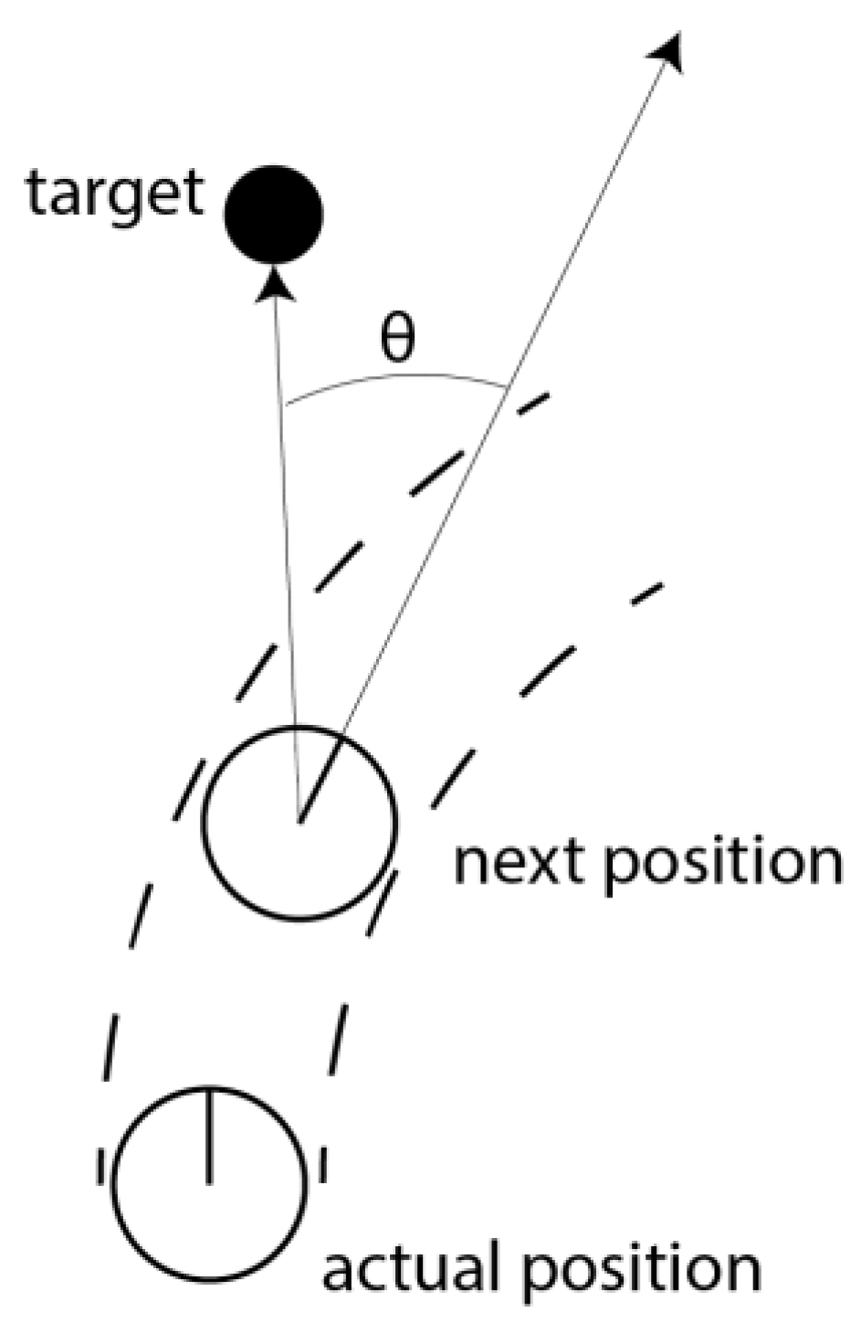
However, the standard DWA does not account for future states, which has led some authors to adopt MPC techniques to select the most suitable trajectory based on multiple parameters, such as the estimated time to reach the goal. The main equation governing the DWA is presented in (Equation (1)), with each variable described in

Table 1. Definition of parameters and variables for the Dynamic Window Approach (DWA), as described in the referenced literature [4]. AGV stands for automated guided vehicle.

Explanation	Variable	Units
Linear velocity of vehicle	${ \mathrm{V}}_r$	m/s
Angular velocity of vehicle	$\dot{\mathsf{\gamma }}$	rad/s
Alignment of the robot with the target direction	$\mathrm{Direction}({\mathrm{V}}_r,\dot{\mathsf{\gamma }})$	-
Proximity to obstacle	$\mathrm{Range}({\mathrm{V}}_r,\dot{\mathsf{\gamma }})$	m
Traversal velocity	$\mathrm{Speed}({\mathrm{V}}_r,\dot{\mathsf{\gamma }})$	m/s
Head factor	${ \mathsf{\alpha }}_{\mathrm{D}}$	rad−1
Obstacle distance confident	${ \mathsf{\beta }}_{\mathrm{D}}$	m−1
Speed coefficient	${ \mathsf{\gamma }}_{\mathrm{D}}$	s/m
Fitness function	$\mathrm{G}({\mathrm{V}}_r, \dot{\mathsf{\gamma }})$	-
Normalization function	$\mathsf{\sigma }$	-

$$\mathrm{G}({\mathrm{V}}_r,\dot{\mathsf{\gamma }})= \mathsf{\sigma }({\mathsf{\alpha }}_{\mathrm{D}}·\mathrm{Direction}({\mathrm{V}}_r,\dot{\mathsf{\gamma }})+{\mathsf{\beta }}_{\mathrm{D}}·\mathrm{Range}({\mathrm{V}}_r,\dot{\mathsf{\gamma }})+{\mathsf{\gamma }}_{\mathrm{D}}·\mathrm{Speed}({\mathrm{V}}_r,\dot{\mathsf{\gamma }}))$$

(1)

The heading is calculated by subtracting θ from 180°, where θ represents the angle between the target point and the AGV’s current heading direction, as illustrated in Figure 1. Additionally, the constants ${\mathsf{\alpha }}_{\mathrm{D}}$, ${\mathsf{\beta }}_{\mathrm{D}}$, and ${\mathsf{\gamma }}_{\mathrm{D}}$ are assigned fixed values of 0.2, 0.2, and 2.0, respectively, as established by Fox et al. [16].

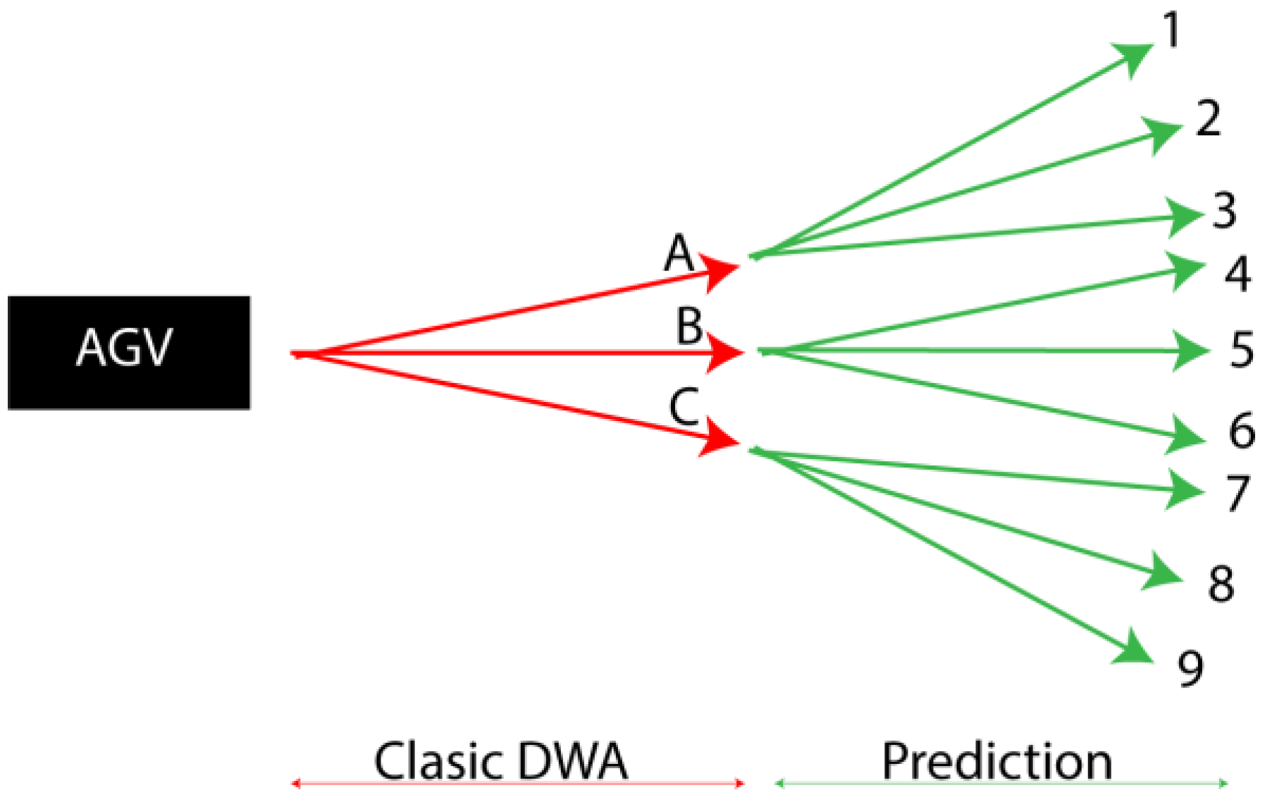
Equation (1) is applied iteratively to generate a variety of candidate trajectories for evaluation. In the traditional DWA framework, this optimization step selects the most suitable path from the set of admissible trajectories. However, to incorporate a predictive component within the Predictive DWA (P-DWA) framework, it becomes necessary to evaluate multiple future possibilities. In this context, the algorithm identifies the three most promising trajectories—labeled A, B, and C—which represent potential future positions for the AGV [24].

After computing the three initial candidate positions (A, B, and C), the process proceeds to the prediction step, which anticipates future movements. In this phase, the DWA algorithm is applied independently to each of the three positions to generate three additional trajectories per candidate, resulting in a total of nine predicted paths. These represent the potential future states of the AGV used for optimization purposes. Among these nine options, the algorithm selects the one with the lowest estimated energy consumption or highest overall score.

It is important to clarify that the AGV physically moves only to one of the initial positions (A, B, or C). For example, if the optimal path is found to originate from the second prediction group, the AGV will proceed to position B. This concept is illustrated in Figure 2.

Traditionally, the Dynamic Window Approach (DWA) allows an Automated Guided Vehicle (AGV) to evaluate and select the optimal path from a set of candidate trajectories, typically labeled A, B, or C. However, with the increasing demand for more sophisticated and energy-efficient autonomous systems, the need for advanced planning techniques has become more apparent. The Predictive Dynamic Window Approach (P-DWA) extends the capabilities of traditional DWA by incorporating future state prediction and energy consumption analysis, resulting in more informed and efficient trajectory selection. Unlike the standard DWA, which optimizes only the immediate next step, P-DWA simulates multiple future steps to anticipate the evolution of the environment. This predictive capability enables the AGV to make decisions that better balance path optimality and energy efficiency by leveraging additional contextual information.

Nevertheless, this approach presents certain challenges. Excessive prediction depth can increase computational complexity and may yield suboptimal outcomes if the environment changes unpredictably during the planning horizon. Therefore, achieving an effective trade-off between prediction depth and computational efficiency is essential for the robust deployment of P-DWA.

The operation of the Predictive Dynamic Window Approach (P-DWA) with integrated energy consumption prediction can be divided into six key steps, each contributing to the AGV’s ability to navigate efficiently and adapt to dynamic environments:

• Trajectory Prediction Using Traditional DWA: The process begins by applying the traditional DWA algorithm to predict multiple candidate trajectories based on the AGV’s current state and environmental perception. From these, the three most promising paths—denoted as points A, B, and C—are selected as potential immediate movement options.
• Motion Simulation: Once the initial trajectories are selected, the AGV’s kinematic model is used to simulate motion toward each of the three points. This ensures trajectory feasibility with respect to physical constraints such as maximum velocity, acceleration, and turning radius.
• Secondary DWA Execution: The DWA algorithm is then applied independently to each of the points A, B, and C to generate three additional trajectories per point. This results in a total of nine possible future paths, expanding the prediction horizon and improving decision robustness.
• Energy Consumption Simulation: The nine candidate trajectories are then evaluated by simulating the AGV’s energy usage along each path. This step is critical for identifying the most energy-efficient option, allowing the AGV to consider not only geometric and dynamic feasibility but also power optimization.
• Optimal Trajectory Selection: Among the nine predicted trajectories, the one with the lowest estimated energy consumption is selected. However, the AGV only physically moves to one of the initial three positions (A, B, or C), as the remaining paths are used solely for predictive evaluation. This strategy mirrors the principles of Model Predictive Control (MPC), focusing on short-term execution while accounting for longer-term outcomes.
• Iterative Execution: This entire process is continuously repeated, enabling the AGV to adapt its navigation strategy in real time. The iterative nature of the algorithm ensures responsiveness to environmental changes and supports consistent energy-efficient operation in dynamic or uncertain scenarios.

The integration of energy-aware prediction into P-DWA introduces several key advantages:

• Improved Decision-Making: By simulating and evaluating future states, the AGV can make more informed navigation decisions, balancing safety, efficiency, and energy constraints.
• Energy Efficiency: Incorporating energy consumption as a decision metric allows the system to prioritize paths that reduce power usage, extending battery life and improving sustainability.
• High Adaptability: The algorithm’s iterative and predictive design enables continuous adaptation to changing environments, ensuring robust performance even in complex, real-world conditions.

Furthermore, to enhance the efficiency of the P-DWA algorithm, the DC motors of the AGV have been mathematically modeled, allowing the required power to be estimated as a function of velocity. For each execution of (Equation (1)), the motor power consumption is calculated. This energy estimation enables the algorithm not only to identify trajectories with optimal speed profiles but also to prioritize those that minimize energy usage, as detailed in (Equation (2)).

$${\omega }_L=\arg \underset{\left\{i\in \left\{A,B,C\right\}\right\}}{min}{E}_i, {\omega }_R=\arg \underset{\left\{i\in \left\{A,B,C\right\}\right\}}{min}{E}_i$$

(2)

The calculation of energy consumption is based on the physical and dynamic properties of the mobile robot. In particular, estimating the power requirements of DC motors is essential for understanding overall system efficiency and ensuring optimal performance. In this study, a mathematical model is proposed to estimate the energy consumption of a robot’s DC motors, taking into account both linear and angular velocities, along with relevant physical parameters such as wheel radius and axle length. This approach aligns with standard formulations for separately excited DC motors, as described in the Control Tutorials for MATLAB and Simulink by the University of Michigan [33], and is consistent with methodologies used in the recent literature on energy-aware motor modeling [34,35].

Specifically, the rotational speeds of the left (${\omega }_L$ and right (${\omega }_R$) wheels are derived from the robot’s linear velocity (${\mathrm{V}}_r$), angular velocity ($\dot{\mathsf{\gamma }}$), and physical dimensions, including the wheel radius (r) and the distance between the wheels (d). The corresponding equations are presented in (Equation (3)). A power constraint of 350 W per motor is imposed to ensure safe operation under typical working conditions and to reflect realistic embedded system limitations, following recommendations observed in prior energy optimization studies for DC motors [35].

$${\omega }_L={\displaystyle \frac{{ \mathrm{V}}_r-\dot{\mathsf{\gamma }}\cdot \frac{d}{2}}{r}}, {\omega }_R={\displaystyle \frac{{ \mathrm{V}}_r+\dot{\mathsf{\gamma }}\cdot \frac{d}{2}}{r}}$$

(3)

Equation (3) describes the differential wheel speeds required for turning maneuvers, where the inner wheel rotates more slowly than the outer wheel. The torque required by each motor (τ) is then calculated by considering the relationship between the motor current (I) and torque, as well as the angular velocity of each motor, as expressed in (Equation (4)).

$${\tau }_L=k_t\cdot I_{L }, {\tau }_R=k_t\cdot I_R$$

(4)

This relationship assumes that torque is directly proportional to current, which is a typical characteristic of DC motors. The power (P) consumed by each motor is calculated by multiplying the torque (τ) by the motor’s angular velocity (ω). The power consumption of the left and right motors is given by (Equation (5)).

$$P_L={\tau }_L\cdot {\omega }_L, P_R={\tau }_R\cdot {\omega }_R$$

(5)

Equation (5) highlights the direct relationship between torque, angular velocity, and power consumption in DC motors. The total energy consumption (E) is then calculated by summing the power consumed by both motors and integrating it over time (t). This is formally expressed in (Equation (6)).

$$E={{\displaystyle \int }}_0^t(P_L+P_R)dt$$

(6)

This equation integrates the power consumption of both motors over time, yielding a comprehensive measure of the system’s energy usage. To ensure safe and reliable operation, each motor is constrained to a maximum power limit of 350 W. This operational constraint is defined in (Equation (7)).

$$P_L={\tau }_L\cdot {\omega }_L\le 350 \mathrm{W}, P_R={\tau }_R\cdot {\omega }_R\le 350 \mathrm{W}$$

(7)

These inequalities ensure that the power consumed by each motor remains within its rated capacity, thereby preventing overheating and potential damage to the system. This constraint is essential for preserving the operational integrity and extending the lifespan of the motors, particularly in dynamic and high-performance applications. Additionally, the complete model of the mobile robot integrates both its kinematic behavior and the relationship between the individual wheel velocities and the robot’s overall motion, as presented in (Equation (8)).

$$\dot{q}=\left[\begin{array}{c}\dot{X}\\ \dot{Y}\\ \dot{\theta }\end{array}\right]=\left[\begin{array}{c}Vr\cdot \cos (\theta )\\ Vr\cdot sin(\theta )\\ \dot{\gamma }\end{array}\right]$$

(8)

where

• $\dot{q}$: the time derivative of the state vector q, which includes the robot’s position (X, Y) and orientation θ.
• θ: the orientation of the robot (in radians), measured from the fixed X-axis.

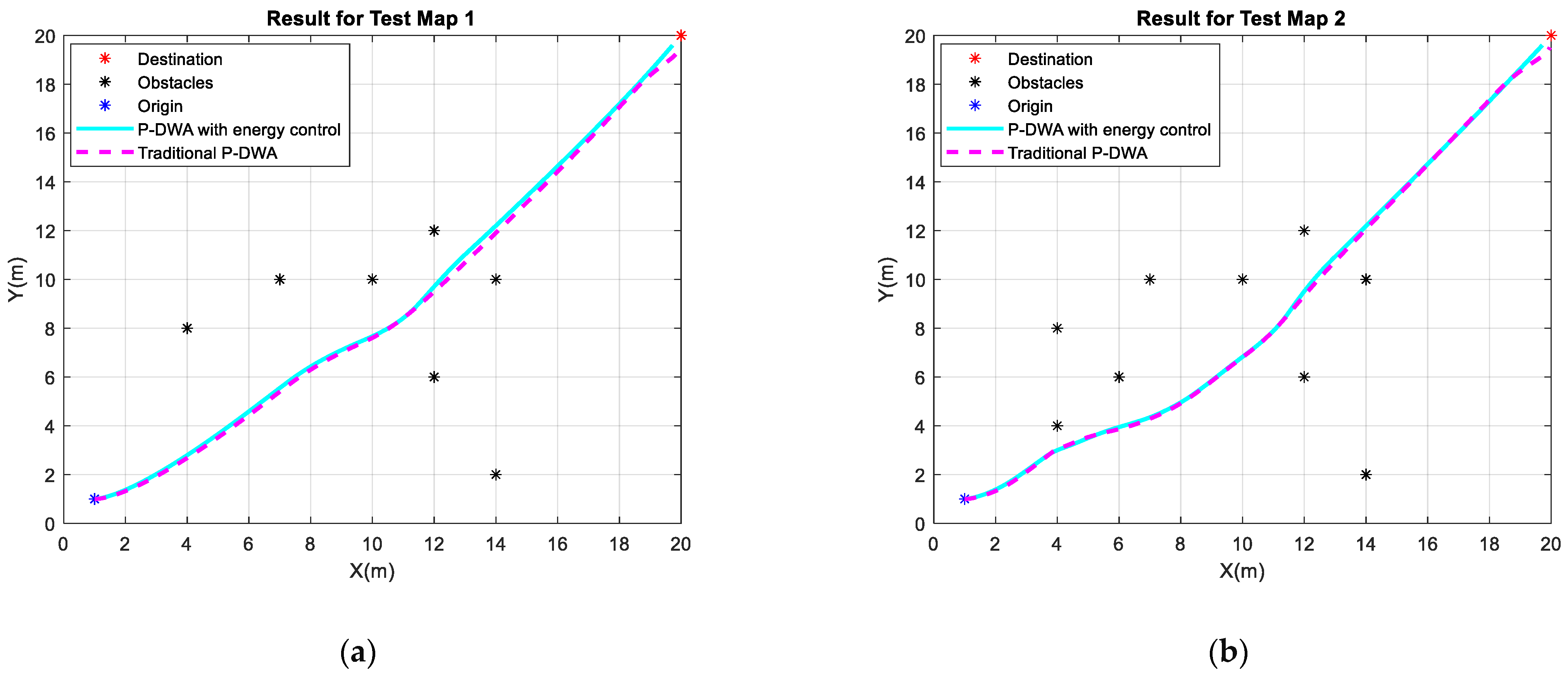
To evaluate the energy management system integrated into the P-DWA algorithm, multiple tests were performed using four distinct map configurations, as illustrated in Figure 3. Each map presents a unique obstacle layout, leading to variations in navigation behavior, including differences in speed profiles, trajectory selection, and energy consumption. This setup enables a detailed comparison between the performance of P-DWA with energy control and the standard P-DWA without it.

• Test Map 1 (a): Contains a sparse distribution of obstacles that influence trajectory selection while maintaining a relatively open navigation space.
• Test Map 2 (b): Modifies the obstacle arrangement from Map 1, introducing alternative path planning challenges and requiring adjustments to the speed profile.
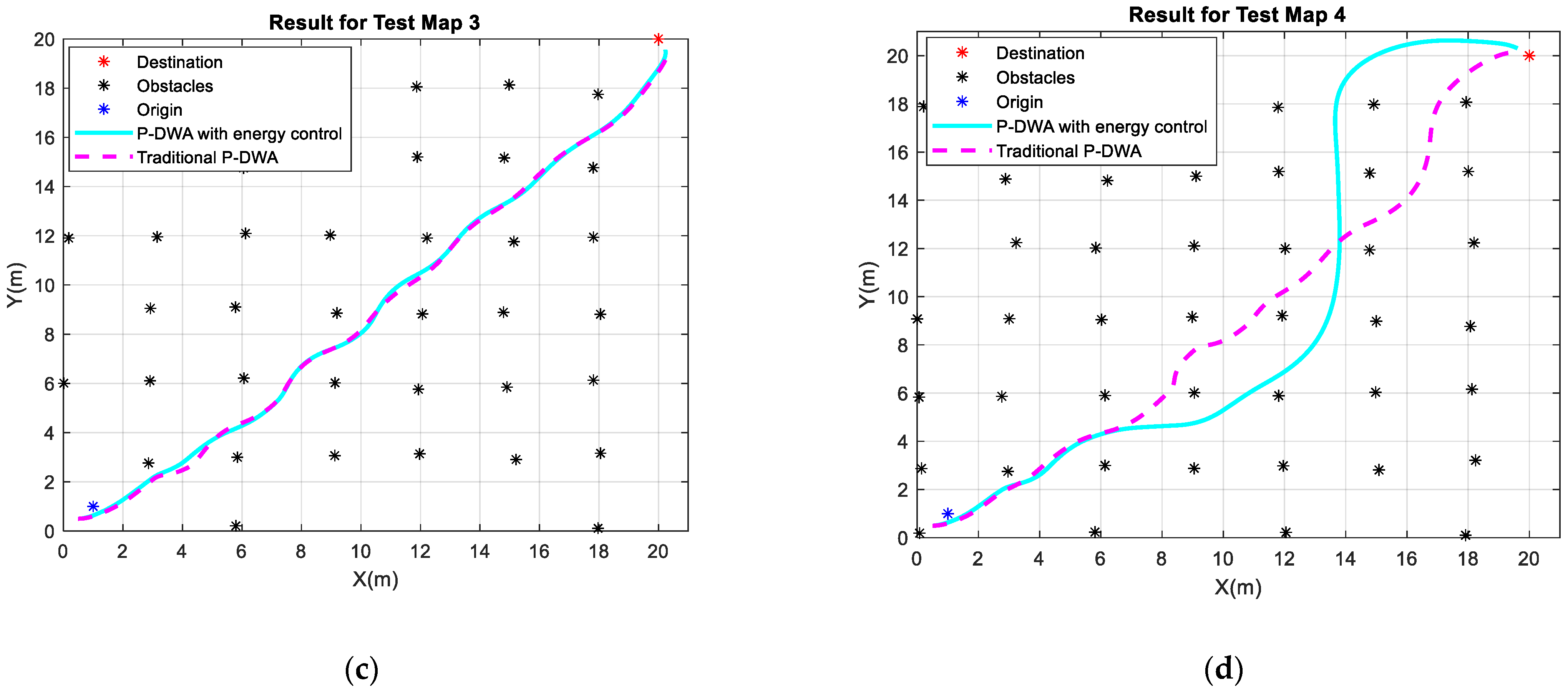
• Test Maps 3 (c): Features a denser and more structured obstacle configuration, significantly constraining movement and demanding more sophisticated energy-aware trajectory planning.
• Test Map 4 (d): Similar to Map 3, but with additional obstacles placed near the starting position. This subtle change increases the initial complexity of navigation, requiring more precise maneuvering and further refinement in energy-optimized path planning.

By analyzing the robot’s behavior across these controlled scenarios, the impact of incorporating energy-aware decision-making into the P-DWA framework can be thoroughly assessed. All experiments were performed using the P-DWA algorithm as an offline trajectory planner, without deploying the strategy on any physical robot. The entire evaluation was carried out in MATLAB R2024b (MathWorks, Natick, MA, USA) on a desktop computer (ASUS, Barcelona, Spain) equipped with an Intel^® Core™ i7-2770K CPU at 3.50 GHz, 20 GB of RAM, and a 64-bit Windows 10 operating system (Microsoft Corp., Redmond, WA, USA). Simulations were executed with a fixed control frequency of 10 Hz, applying a control step (dt) of 0.05 s, a maximum linear velocity of 3 m/s and a maximum angular velocity of 2 rad/s. The prediction horizon was limited to 2.5 s to maintain computational tractability while ensuring planning fidelity. All motion data, including velocity profiles, trajectory paths, and energy metrics, were recorded for post-analysis.

3. Results and Discussions

As shown in Figure 3, the two algorithms exhibit distinct behaviors across the four test maps. A detailed analysis of each case is presented below to assess the effectiveness of the energy-aware P-DWA in terms of navigation behavior. This analysis aims to provide deeper insights into the performance of the integrated energy control mechanism and its overall impact on system efficiency and trajectory quality.

As shown in Figure 3a–c, the first three test cases reveal nearly identical trajectories for both algorithms. This similarity arises because the dynamic weighting parameters (${\mathsf{\gamma }}_{\mathrm{D}}$, ${\mathsf{\beta }}_{\mathrm{D}}$, and ${\mathsf{\alpha }}_{\mathrm{D}}$) remain constant, ensuring that the decision-making processes for obstacle avoidance and path selection are fundamentally equivalent. However, beneath this apparent similarity lies a critical difference: energy consumption.

In contrast, Test Map 4 (Figure 3d) introduces a subtle yet impactful variation—two additional obstacles placed near the starting point, slightly altering the navigable area. This change results in a more pronounced divergence in behavior between the two algorithms, particularly in their capacity to adapt to constrained environments.

A key consideration is that the energy-aware P-DWA utilizes a prediction window that may suggest an alternative trajectory appearing more efficient at first. However, these predicted paths require validation, as substantial deviations from the traditional trajectory—as well as factors such as increased travel distance—can affect their overall viability. In certain situations, an energy-optimized route may not be the most practical when additional environmental constraints are considered.

This highlights a fundamental requirement of the P-DWA framework: the need for additional filtering layers in the trajectory planning process. These layers would serve to eliminate non-viable paths and ensure a balanced trade-off between energy efficiency and overall feasibility. Such an approach underscores the necessity of a more sophisticated, multi-criteria decision-making process in energy-aware navigation systems.

To fully understand these differences, trajectory analysis alone is insufficient. For this reason, Figure 4, Figure 5, Figure 6 and Figure 7 provide a detailed examination of energy consumption along each path. The total energy expenditure, discussed in the following analysis, is obtained by summing the energy consumed at each iteration, as defined in Equation (6). This comprehensive evaluation provides deeper insights into the advantages of incorporating energy control into the P-DWA framework.

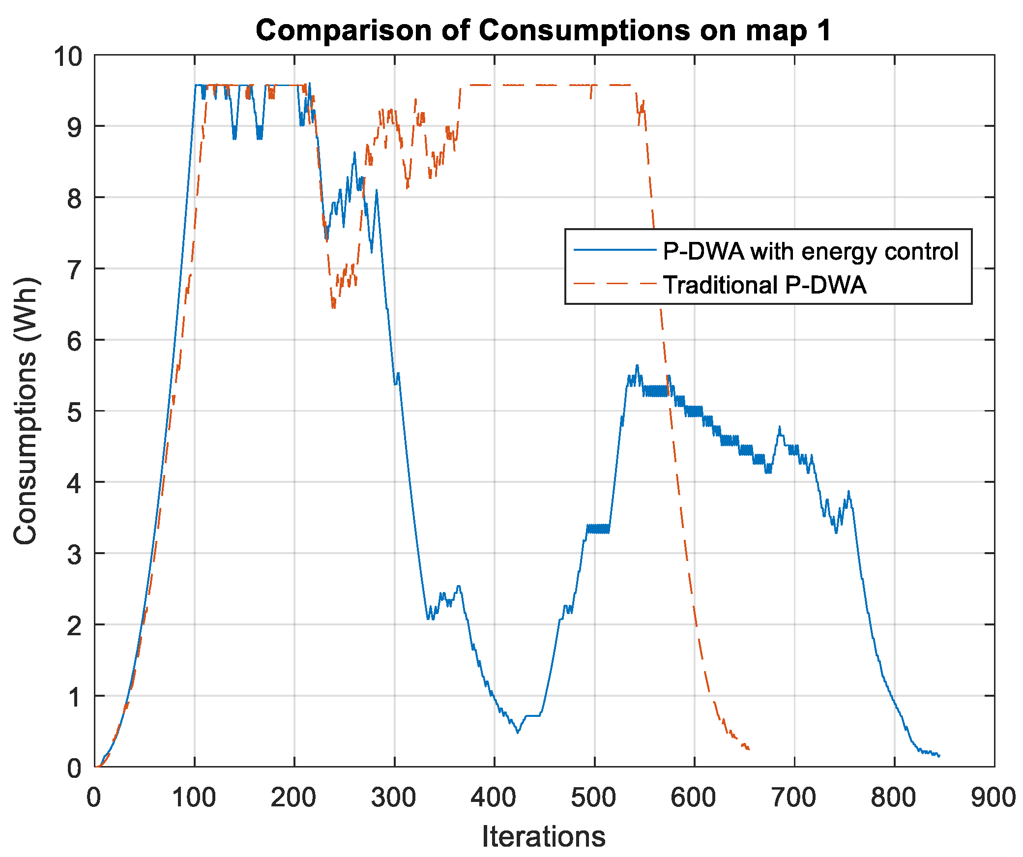
As illustrated in Figure 4, the energy consumption profiles for both algorithms on Test Map 1 differ substantially. The energy-aware P-DWA requires approximately 200 additional iterations compared to the traditional method, resulting in a time increase of about 10 s. This is attributed to the algorithm’s prioritization of energy efficiency over rapid completion.

A key observation is that the traditional P-DWA maintains a relatively high and stable energy consumption throughout most of the trajectory, followed by a sharp drop after approximately iteration 550, signaling premature completion of the route. This behavior indicates that the traditional approach emphasizes direct navigation without active optimization of energy usage, leading to a higher peak consumption of nearly 9.5 Wh during operation.

In contrast, the energy-aware P-DWA exhibits a more gradual and adaptive consumption profile, characterized by multiple reductions in power usage throughout the trajectory. This suggests that the algorithm actively regulates velocity and acceleration to reduce unnecessary energy expenditure. Notably, after iteration 400, the algorithm executes a significant energy-saving maneuver, likely involving speed reduction or smoother trajectory adjustment. This behavior reflects a more controlled and efficient energy management strategy.

The total energy consumption further emphasizes this distinction:

• Traditional P-DWA: 4.67 Wh, with a sharp energy decline near the end of the trajectory.
• Energy-aware P-DWA: 3.70 Wh, with a smoother and more balanced energy profile across the iterations

This represents a 21% reduction in total energy consumption, reinforcing the effectiveness of the proposed approach in optimizing energy use. While the traditional P-DWA completes the trajectory more quickly, it does so at the cost of significantly higher energy consumption. In contrast, the energy-aware method requires more iterations but ensures a more sustainable and controlled energy expenditure.

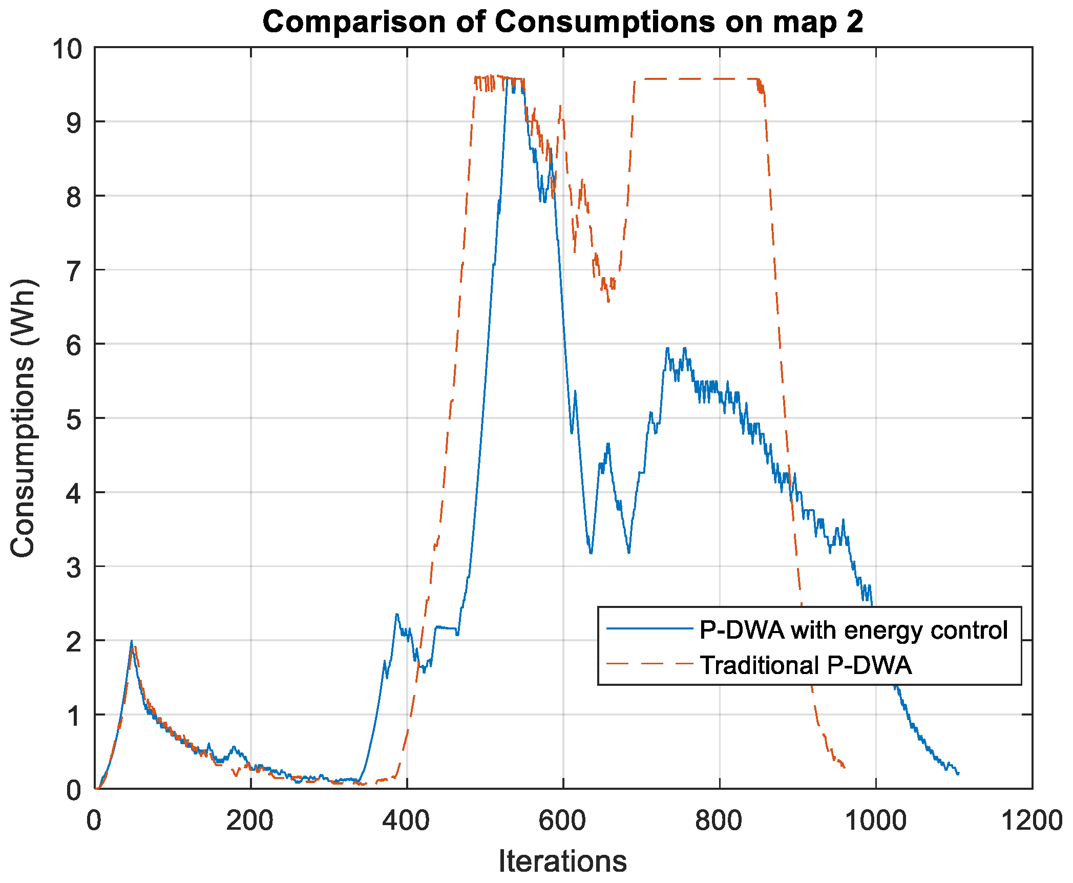
In the second scenario, corresponding to Figure 3b and illustrated in the results of Figure 5, a similar behavioral trend is observed. In this case, the proposed P-DWA with energy control achieves a lower overall energy expenditure compared to the traditional P-DWA algorithm. The total energy consumption for each approach is as follows:

• P-DWA with energy control: 3.16 Wh
• Traditional P-DWA: 4.17 Wh

This represents a 24% reduction in energy consumption, reinforcing the effectiveness of integrating energy-aware decision-making into motion planning. The proposed method demonstrates a more gradual and controlled energy consumption profile, avoiding sharp peaks and unnecessary energy usage. In contrast, the traditional P-DWA exhibits a high-consumption pattern followed by an abrupt completion of the trajectory, suggesting less efficient energy management.

Despite the energy savings, the traditional P-DWA completes the trajectory with fewer iterations, once again highlighting a trade-off between energy efficiency and execution time. The proposed method requires approximately 12 additional seconds to complete the navigation task, which may be a relevant factor depending on the specific application. However, in scenarios where energy conservation is critical, this additional time is a minor cost in exchange for the substantial reduction in power consumption.

This balance between execution time and energy optimization suggests that the proposed approach is particularly well-suited for applications involving battery-powered autonomous systems, automated guided vehicles, and mobile robots, where extending operational time is a priority. The results presented in Figure 4 and Figure 5 further validate the benefits of incorporating energy-aware motion planning, positioning the proposed algorithm as a promising advancement in the field of energy-efficient robotic navigation.

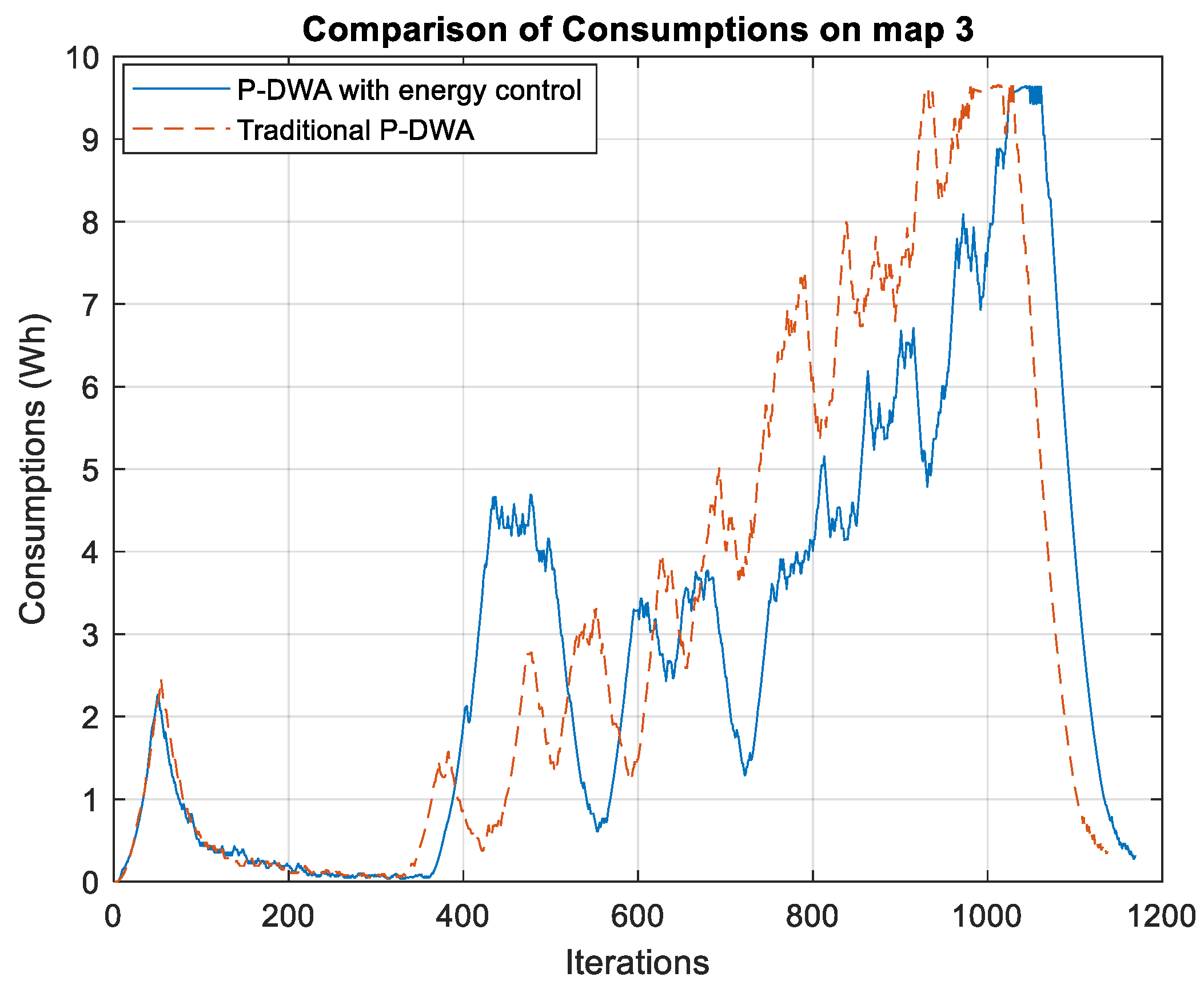
Figure 6 presents the energy consumption profiles of both algorithms on Test Map 3, revealing a trend that differs from the previous scenarios. Unlike earlier cases where the proposed P-DWA with energy control achieved substantial energy savings, the difference between the two approaches here is less pronounced. The total energy consumption for each method is as follows:

• P-DWA with energy control: 3.4 Wh
• Traditional P-DWA: 3.6 Wh

This yields a modest reduction of approximately 5.6% in energy consumption using the energy-aware method. The smaller difference suggests that in this particular map configuration, the trajectory generated by the traditional P-DWA is already relatively efficient, resulting in similar energy expenditures for both approaches.

However, a closer examination of the energy consumption patterns across iterations reveals noteworthy distinctions. While the traditional P-DWA initially maintains lower energy consumption, it experiences a sharp increase toward the end of the trajectory, peaking at nearly 9.5 Wh before abruptly dropping upon completion. In contrast, the proposed P-DWA exhibits a more progressive and adaptive consumption profile, avoiding sudden peaks and distributing energy use more evenly throughout the navigation process. This behavior reflects a more consistent and optimized decision-making strategy that emphasizes energy efficiency across the entire trajectory, rather than at isolated segments.

As observed in earlier test cases, the proposed P-DWA requires more iterations to complete the trajectory, further illustrating the trade-off between energy efficiency and execution time. However, in this specific scenario, the additional iterations do not yield a substantial improvement in total energy savings.

These findings suggest that while the energy-aware P-DWA promotes a more stable and controlled energy distribution, its overall impact on energy consumption is highly dependent on obstacle layout and path complexity. The results emphasize that the benefits of energy-aware motion planning are more evident in certain environments. Nonetheless, the algorithm’s ability to avoid abrupt power spikes and maintain consistent energy usage remains a valuable characteristic—particularly in applications where power fluctuations may compromise system stability, such as in autonomous mobile robots and battery-powered vehicles.

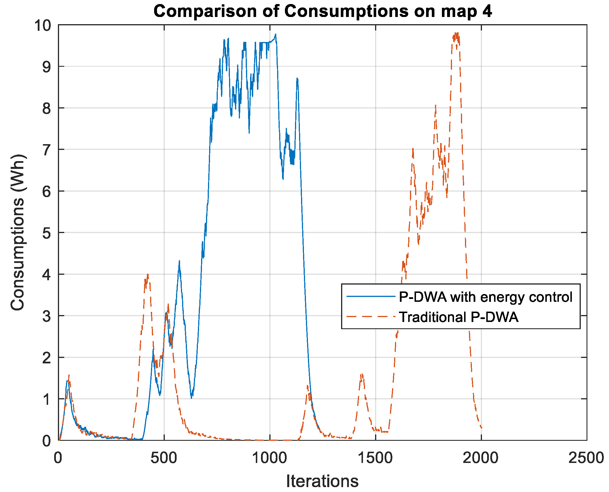
Figure 7 illustrates the energy consumption profiles for both algorithms on Test Map 4, where a notable difference in trajectory length between the two approaches can be observed. Unlike previous cases, the proposed P-DWA with energy control follows a significantly longer path, as depicted in the corresponding trajectory plot. This extended trajectory directly impacts the energy consumption results, exhibiting a reverse trend compared to the earlier scenarios. The total energy consumption for each algorithm is as follows:

• P-DWA with energy control: 4.7 Wh
• Traditional P-DWA: 3.02 Wh

In contrast to the previous test cases—where the energy-aware algorithm consistently reduced overall energy usage—in this scenario, it results in higher total consumption. This outcome is primarily due to the longer trajectory selected by the proposed method, which increases the number of iterations and, consequently, the cumulative energy expenditure. An analysis of the trajectory plot reveals that the energy-aware P-DWA opts for a smoother and more curved path, potentially aiming to optimize velocity and minimize abrupt acceleration or braking. However, this smoother profile leads to an extended travel distance, ultimately increasing total energy use.

It is important to note that this outcome stems from the nature of the trajectory planning approach used. Since the method performs simulation-based evaluation of multiple possible paths, it selects those that prioritize energy profile smoothness over minimum travel distance. In a real-time or reactive context, additional logical constraints would likely discard such elongated trajectories. Thus, this result highlights the role of the planner when unconstrained by time or sensor feedback logic and suggests the need to integrate further trajectory selection constraints when deploying in more dynamic or resource-limited environments.

Conversely, the traditional P-DWA follows a more direct route, completing the task in fewer iterations and consuming less overall energy, despite displaying less control over power spikes. The energy consumption graph further supports this observation: the traditional method shows a late, high-intensity energy spike, while the energy-aware algorithm distributes its consumption more evenly over time.

These findings highlight a critical trade-off between trajectory optimization and total energy efficiency. Although the energy-aware P-DWA effectively manages power fluctuations and avoids sharp peaks, its extended path may result in higher total energy consumption—an outcome that may not be ideal in all use cases. Therefore, selecting between these two approaches should depend on the specific operational priorities: whether minimizing energy usage per unit of time or reducing overall energy expenditure across the entire trajectory is more critical to the application.

Table 2. Performance metrics and computational cost for proposed and traditional navigation algorithms.

Scenario	Algorithm	Distance (m)	Mean (m/s) Velocity	Median (m/s) Velocity	Total Simulation Time (s)	Avg Iteration Time (ms)
1	Proposed	26.73	0.6	0.68	13.36	16.70
1	Traditional	26.83	0.8	0.98	10.27	15.64
2	Proposed	26.97	0.49	0.49	18.37	16.68
2	Traditional	27.07	0.57	0.52	15.38	15.98
3	Proposed	28.31	0.49	0.52	21.04	18.50
3	Traditional	28.17	0.50	0.48	20.17	17.74
4	Proposed	32.42	0.53	0.51	22.02	17.80
4	Traditional	28.69	0.29	0.17	35.31	17.64

summarizes the mean and median speeds recorded for both algorithms across the four test scenarios, offering a comparative analysis of their performance. While one reviewer noted that speed is the primary factor influencing the differences between the two approaches, it is important to emphasize that both speed and acceleration significantly contribute to the observed outcomes. The similarity in trajectory planning between the two methods is largely due to the consistent configuration parameters used in the P-DWA. The only modification introduced in the proposed algorithm is the additional constraint related to energy consumption.

As shown in Figure 3a and Table 2, the proposed energy-aware algorithm achieves a mean speed of 0.6 m/s and a median speed of 0.68 m/s over a trajectory of 26.73 m, whereas the traditional P-DWA reaches higher values of 0.8 m/s and 0.98 m/s over a comparable distance of 26.83 m. Despite its lower speed, the proposed algorithm maintains a simulation time of 13.36 s with an average iteration time of 16.70 ms, indicating a modest computational load. The traditional algorithm, although faster in execution (10.27 s), only slightly improves iteration efficiency (15.64 ms), highlighting that the energy-aware strategy introduces minimal computational overhead. The higher median relative to mean speed in the traditional method suggests a more aggressive acceleration pattern, potentially leading to increased energy demand and less stable movement.

In the second test case (Figure 3b), both algorithms reduce speed due to obstacle interference at (4, 4) and (6, 6), which significantly constrains motion. The proposed method maintains both mean and median speeds at 0.49 m/s, while the traditional algorithm achieves a higher mean (0.57 m/s) and median (0.52 m/s). The distances traveled are similar (26.97 m vs. 27.07 m), yet the proposed algorithm takes longer to simulate (18.37 s vs. 15.38 s), primarily due to more conservative acceleration profiles. Computationally, the difference remains modest (16.68 ms vs. 15.98 ms per iteration), confirming that the energy-aware logic does not drastically increase per-step computational cost.

In the third scenario (Figure 3c), performance between methods converges. The proposed algorithm registers 0.49 m/s mean and 0.52 m/s median speeds, covering 28.31 m in 21.04 s with an average iteration time of 18.50 ms. The traditional P-DWA reaches 0.50 m/s and 0.48 m/s over a similar 28.17 m trajectory, completing in 20.17 s with a 17.74 ms average iteration time. The marginal differences suggest that both algorithms follow nearly identical trajectories, with the proposed method slightly favoring smoother velocity transitions at the cost of marginally longer computation time.

In the final test case (Figure 3d), a significant divergence arises. The energy-aware method covers a longer distance (32.42 m vs. 28.69 m) while sustaining higher speeds (0.53 m/s mean, 0.51 m/s median). The traditional algorithm, by contrast, demonstrates considerably lower performance (0.29 m/s mean and 0.17 m/s median), completing its trajectory in 35.31 s—far longer than the proposed method’s 22.02 s. Despite this, iteration times are comparable (17.80 ms vs. 17.64 ms), again supporting the idea that energy regulation comes at minimal computational cost. The extended trajectory of the proposed algorithm may result in higher total energy usage, but the smoother motion profile contributes to better control and adaptability.

Overall, both trajectory dynamics and computational efficiency must be considered jointly. The proposed algorithm consistently demonstrates stable behavior with only slightly higher iteration times (typically within 1 ms of the traditional method), ensuring real-time feasibility. The extended simulation durations observed are primarily due to lower speeds and longer trajectories, not to inefficient computation.

These findings reinforce the notion that energy-aware navigation does not compromise computational viability. On the contrary, it offers smoother control and predictable iteration costs while balancing speed and distance effectively. This makes it an appealing choice in energy-constrained or safety-critical applications where smooth trajectories and predictable energy profiles are prioritized over minimal travel time. Scenario 4 especially highlights the trade-off between trajectory length and energy stability, reminding us that the optimal strategy depends on application goals—be it minimizing energy usage, improving execution time, or ensuring robustness.

4. Conclusions

The results demonstrate the distinct behaviors of the traditional and the proposed energy-controlled Predictive Dynamic Window Approach (P-DWA) across diverse navigation conditions. The analysis highlights the trade-offs between speed, acceleration, energy efficiency, and trajectory planning, revealing that although the traditional algorithm achieves higher mean and median speeds, it does so at the cost of greater energy consumption and more abrupt acceleration patterns. These sharp variations result in higher energy peaks, which reduce efficiency in energy-sensitive or battery-powered robotic applications. In contrast, the proposed energy-aware P-DWA prioritizes smoother acceleration and more consistent energy distribution, achieving significant reductions in energy consumption without critically compromising execution time.

Quantitatively, the proposed algorithm achieved a 22% reduction in energy consumption in Scenario 1 and 24% in Scenario 2, while maintaining similar distances and total simulation times. In Scenario 3, the energy savings were minimal—just 2.1%—indicating that when the trajectory is already efficient, energy-aware constraints offer limited additional benefits. In Scenario 4, however, the proposed method consumed approximately 56% more energy than the traditional one, due to an elongated trajectory. This case illustrates an important trade-off: while energy-aware strategies reduce consumption in most conditions, they may increase total distance traveled in complex environments, potentially offsetting their benefits.

These findings confirm that acceleration control is as critical as speed in determining energy efficiency. While the traditional algorithm emphasizes faster traversal, often with sharp changes in velocity, the proposed planner focuses on regulated motion, resulting in lower peak demands and smoother profiles. This validates the energy-aware P-DWA as a robust solution for applications where energy efficiency is essential, particularly in long-duration, battery-constrained missions.

Future work should focus on evaluating the impact of the proposed planner not only on energy performance but also on trajectory fidelity. Since the energy-aware algorithm acts as a local planner within a broader navigation architecture, it is crucial to analyze whether energy-optimized local paths deviate significantly from the global plan. A systematic study of such deviations, particularly under high constraint conditions, will help quantify whether the extended trajectories remain within acceptable operational limits. Understanding this relationship will be key to integrating energy-aware motion planning seamlessly into full navigation stacks, ensuring both energy efficiency and mission reliability.