
Study on the Evolution of Groundwater Level in Hebei Plain to the South of Beijing and Tianjin Based on LSTM Model

Abstract
1. Introduction
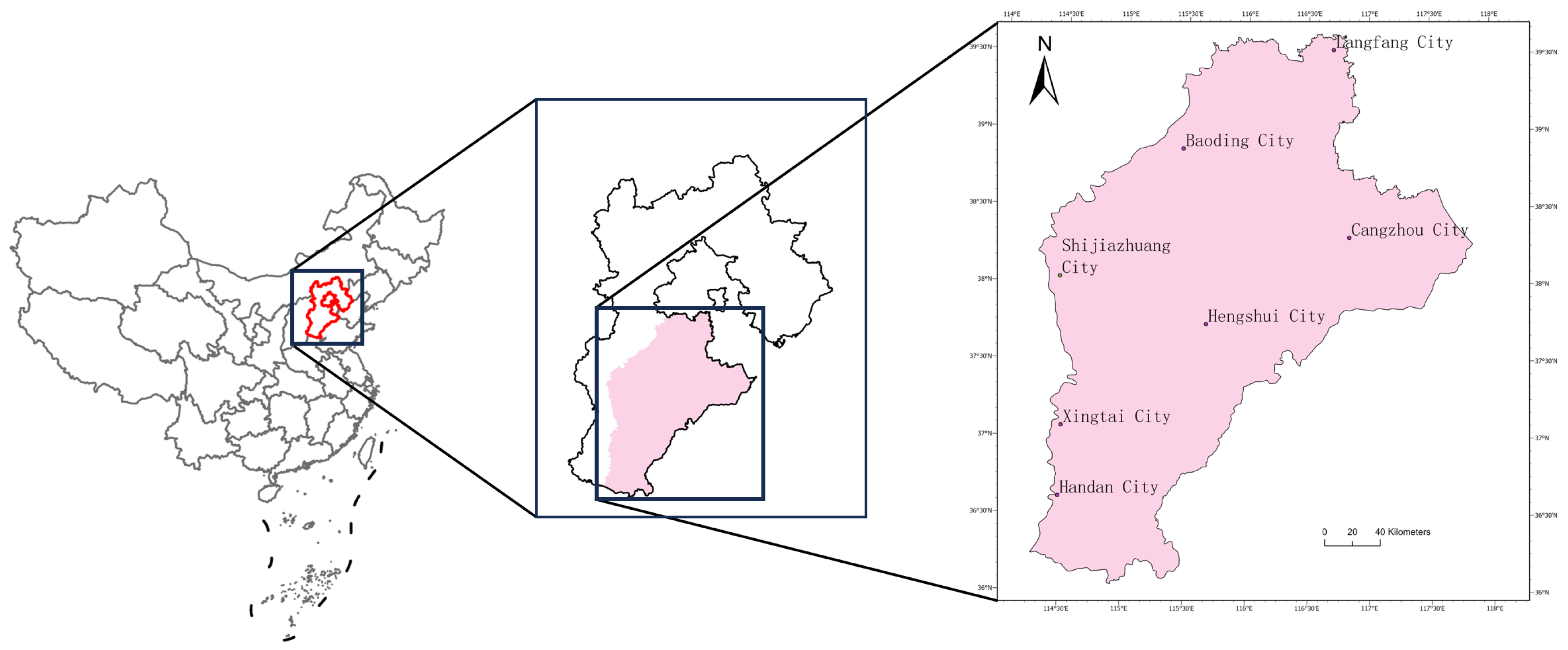
2. Study Area
3. Materials and Methods
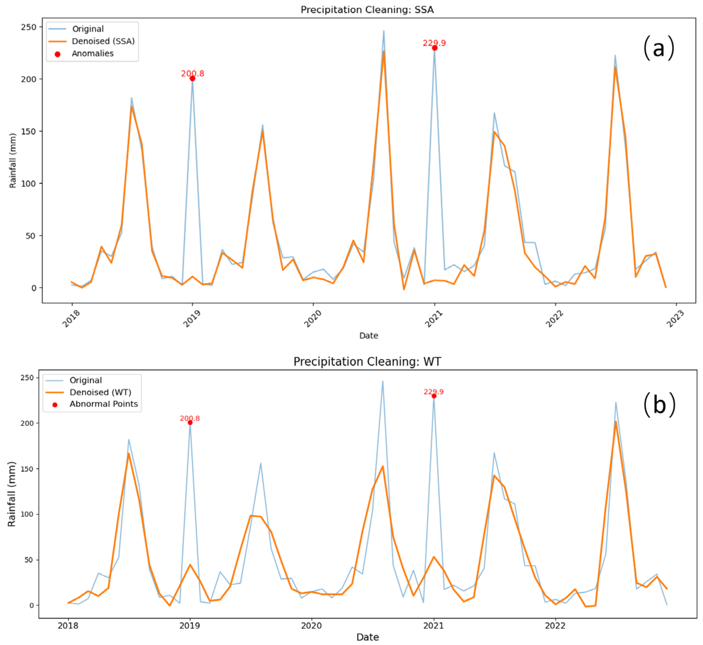
3.1. Data Sources and Processing
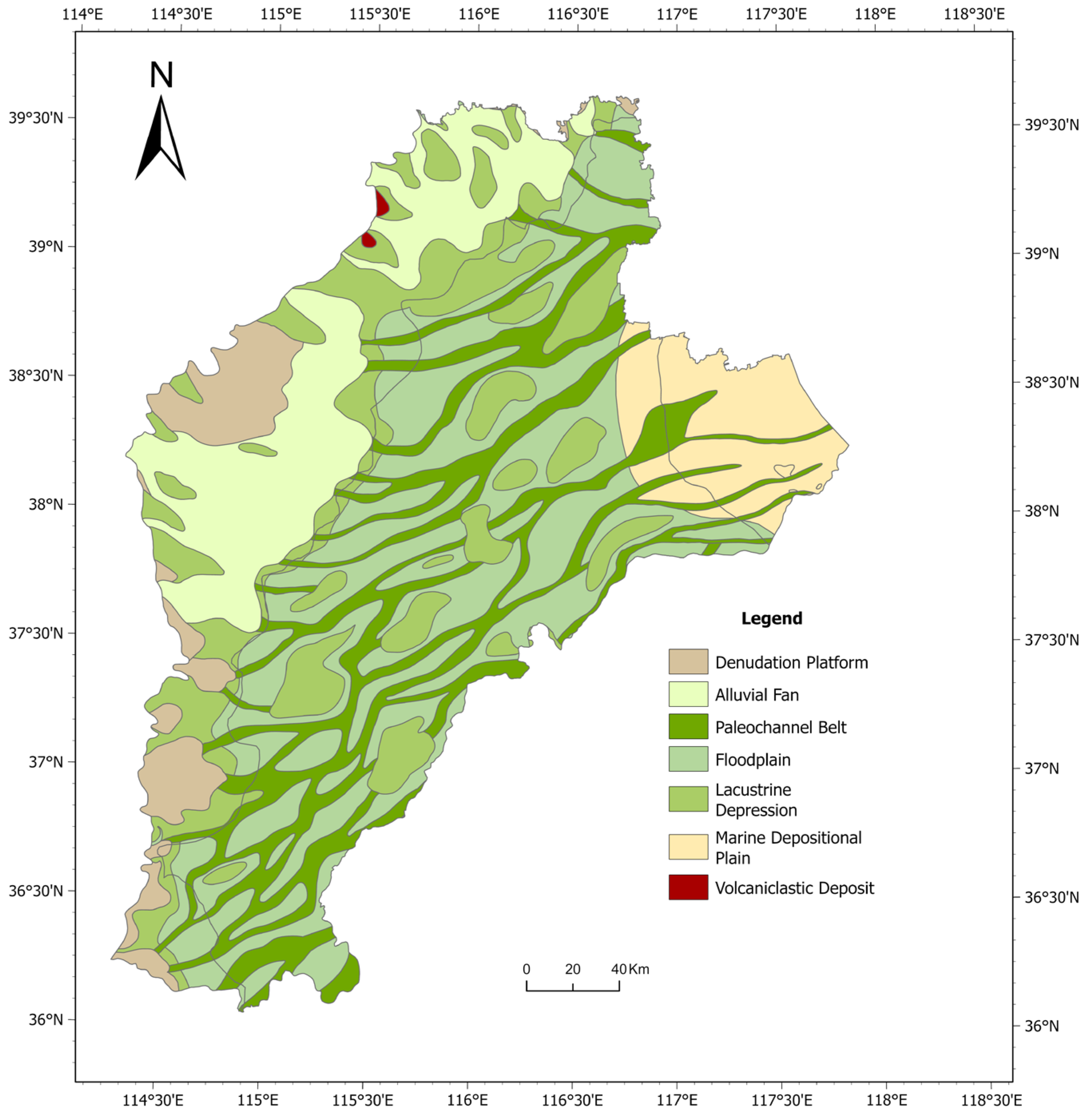
3.2. Sample Division Based on Depositional Systems
3.3. Model Construction
3.4. Hyperparameter Settings
3.5. Assessment Methodology
4. Results
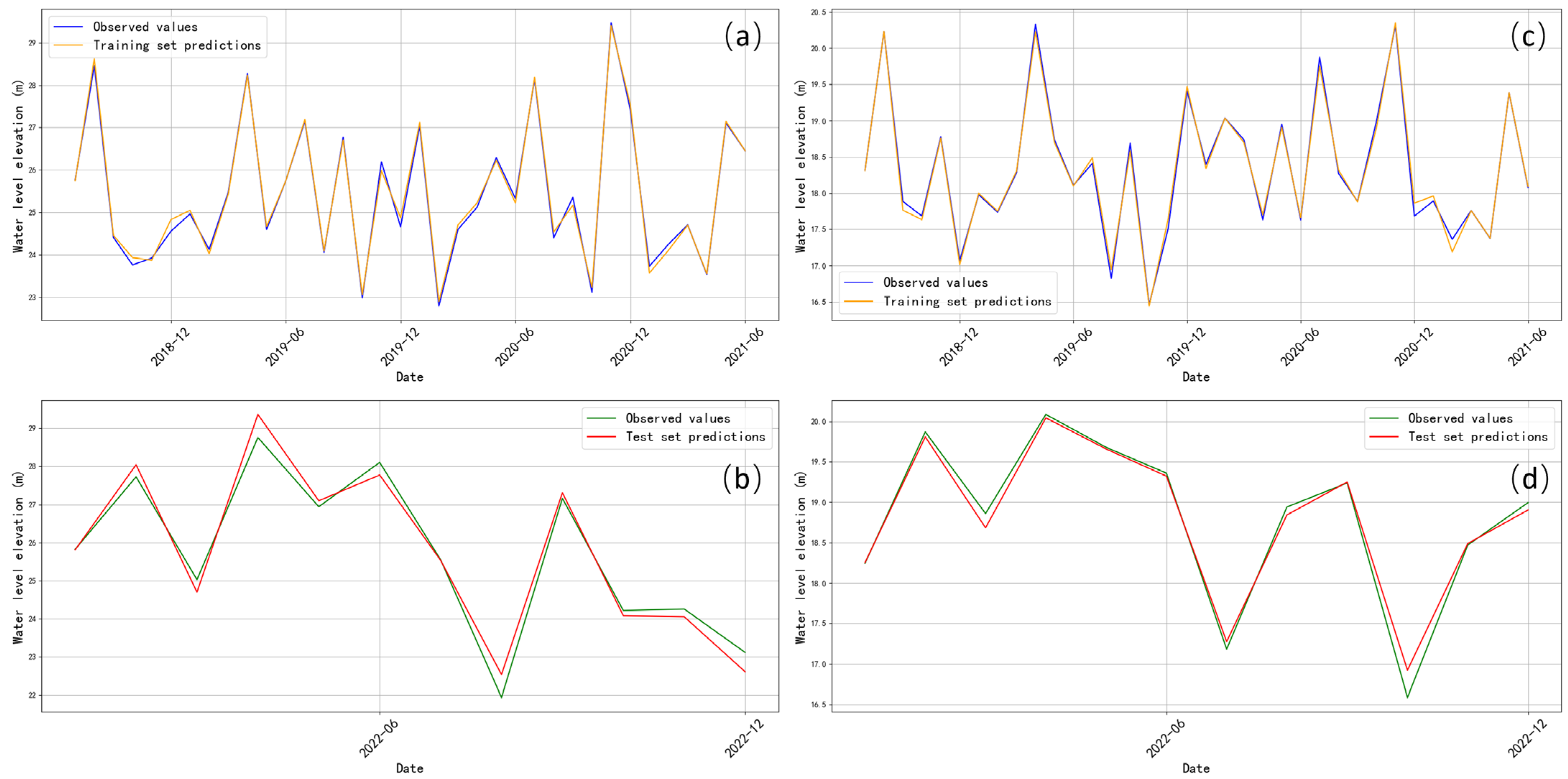
4.1. Fitting Result
4.2. Groundwater Level Prediction Results
4.2.1. Scenario Setting for the Forecast Period
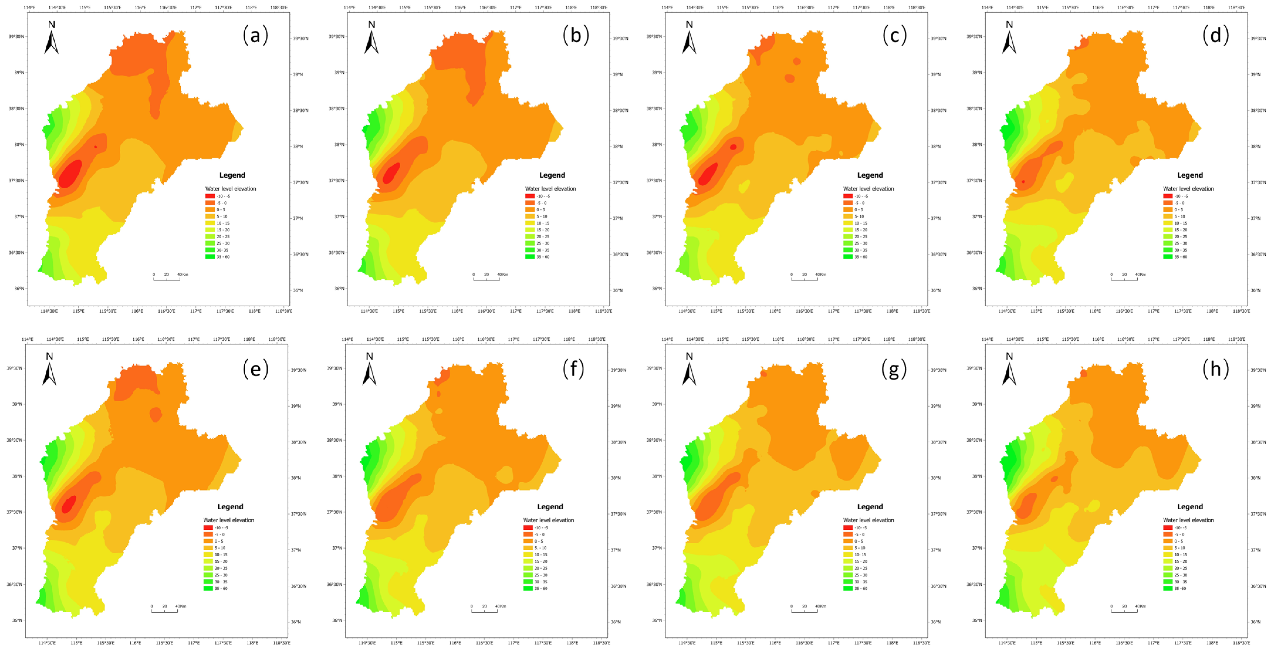
4.2.2. Predicted Results
5. Discussion
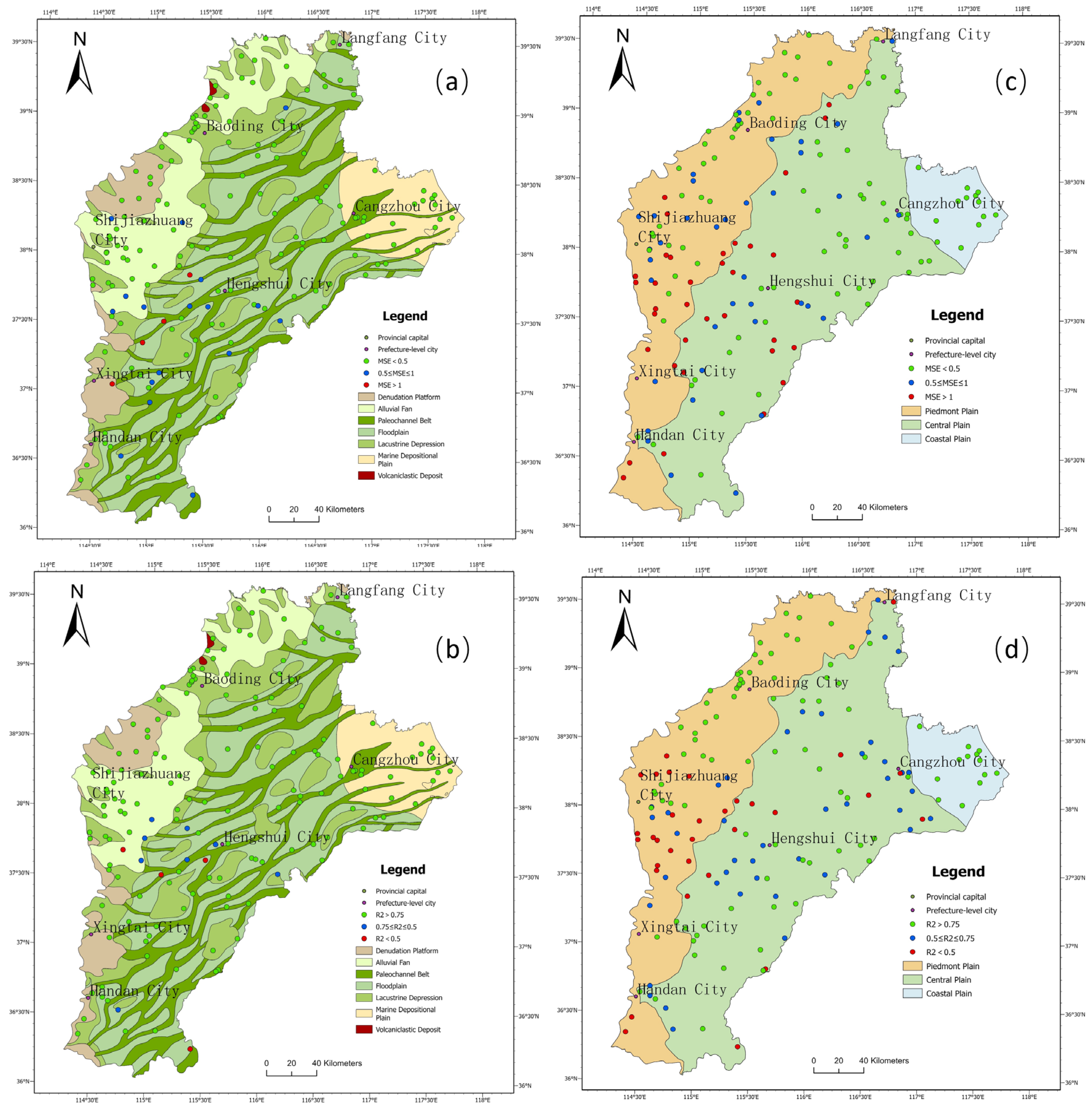
5.1. Comparison of Simple vs. Refined Partitioning
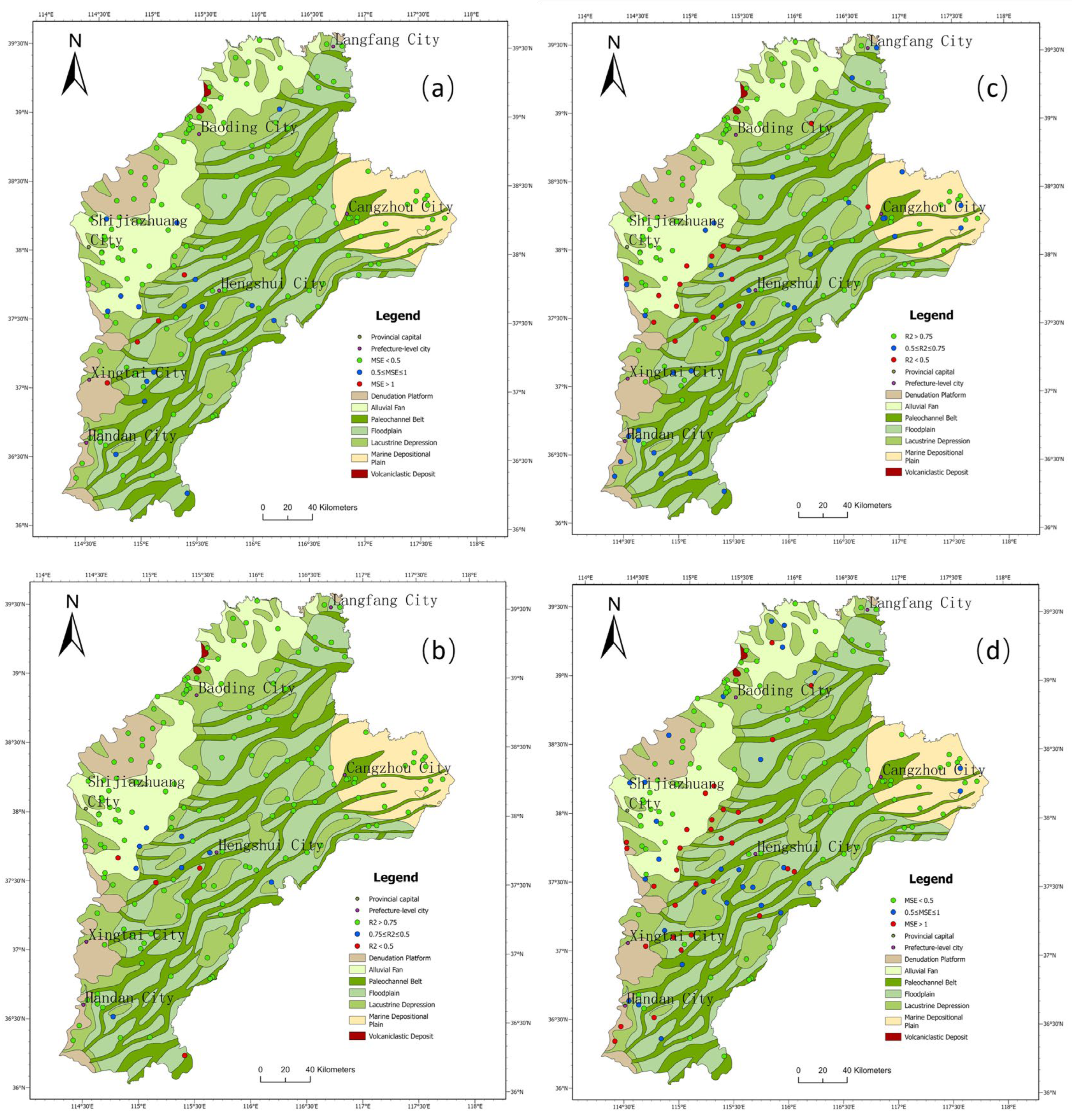
5.2. Comparison of Models with and Without Static Features
6. Conclusions
Author Contributions
Funding
Institutional Review Board Statement
Informed Consent Statement
Data Availability Statement
Acknowledgments
Conflicts of Interest
References
- Chen, F.; Xu, X.; Yang, Y.; Ding, Y.; Li, J.; Li, Y. Investigation on the evolution trends and influencing factors of groundwater resources in China. Adv. Water Sci. 2020, 31, 811–819. [Google Scholar] [CrossRef]
- Usman, M.; Qamar, M.U.; Becker, R.; Zaman, M.; Conrad, C.; Salim, S. Numerical modelling and remote sensing based approaches for investigating groundwater dynamics under changing land-use and climate in the agricultural region of Pakistan. J. Hydrol. 2020, 581, 124408. [Google Scholar] [CrossRef]
- Ma, Z.; Wang, W.; Hou, X.; Wang, J.; Duan, L.; Wang, Y.; Zhao, M.; Li, J.; Jing, J.; Li, L. Examining the change in groundwater flow patterns: A case study from the plain area of the Baiyangdian Lake Watershed, North China. J. Hydrol. 2023, 625, 130160. [Google Scholar] [CrossRef]
- Lachaal, F.; Mlayah, A.; Bédir, M.; Tarhouni, J.; Leduc, C. Implementation of a 3-D groundwater flow model in a semi-arid region using MODFLOW and GIS tools: The Zéramdine–Béni Hassen Miocene aquifer system (east-central Tunisia). Comput. Geosci. 2012, 48, 187–198. [Google Scholar] [CrossRef]
- Huang, J.; Zhou, Y.; Wenninger, J.; Ma, H.; Zhang, J.; Zhang, D. How water use of Salix psammophila bush depends on groundwater depth in a semi-desert area. Environ. Earth Sci. 2016, 75, 556. [Google Scholar] [CrossRef]
- Roy, P.K.; Roy, S.S.; Giri, A.; Banerjee, G.; Majumder, A.; Mazumdar, A. Study of impact on surface water and groundwater around flow fields due to changes in river stage using groundwater modeling system. Clean Technol. Environ. Policy 2015, 17, 145–154. [Google Scholar] [CrossRef]
- Osman, A.I.A.; Ahmed, A.N.; Chow, M.F.; Huang, Y.F.; El-Shafie, A. Extreme gradient boosting (Xgboost) model to predict the groundwater levels in Selangor Malaysia. Ain Shams Eng. J. 2021, 12, 1545–1556. [Google Scholar] [CrossRef]
- Demirel, M.C.; Venancio, A.; Kahya, E. Flow forecast by SWAT model and ANN in Pracana basin, Portugal. Adv. Eng. Softw. 2009, 40, 467–473. [Google Scholar] [CrossRef]
- Hsu, K.; Gupta, H.; Sorooshian, S. Artificial neural network modeling of the rainfall-runoff process. Water Resour. Res. 1995, 31, 2517–2530. [Google Scholar] [CrossRef]
- Kratzert, F.; Klotz, D.; Brenner, C.; Schulz, K.; Herrnegger, M. Rainfall–runoff modelling using long short-term memory (LSTM) networks. Hydrol. Earth Syst. Sci. 2018, 22, 6005–6022. [Google Scholar] [CrossRef]
- Lees, T.; Buechel, M.; Anderson, B.; Slater, L.; Reece, S.; Coxon, G.; Dadson, S.J. Benchmarking data-driven rainfall–runoff models in Great Britain: A comparison of long short-term memory (LSTM)-based models with four lumped conceptual models. Hydrol. Earth Syst. Sci. 2021, 25, 5517–5534. [Google Scholar] [CrossRef]
- Yang, S.; Yang, D.; Chen, J.; Santisirisomboon, J.; Lu, W.; Zhao, B. A physical process and machine learning combined hydrological model for daily streamflow simulations of large watersheds with limited observation data. J. Hydrol. 2020, 590, 125206. [Google Scholar] [CrossRef]
- Li, B.; Li, R.; Sun, T.; Gong, A.; Tian, F.; Khan, M.Y.A.; Ni, G. Improving LSTM hydrological modeling with spatiotemporal deep learning and multi-task learning: A case study of three mountainous areas on the Tibetan Plateau. J. Hydrol. 2023, 620, 129401. [Google Scholar] [CrossRef]
- Zounemat-Kermani, M.; Batelaan, O.; Fadaee, M.; Hinkelmann, R. Ensemble machine learning paradigms in hydrology: A review. J. Hydrol. 2021, 598, 126266. [Google Scholar] [CrossRef]
- Nearing, G.S.; Kratzert, F.; Sampson, A.K.; Pelissier, C.; Klotz, D.; Frame, J.M.; Prieto, C.; Gupta, H.V. What Role Does Hydrological Science Play in the Age of Machine Learning? Water Resour. Res. 2020, 57, e2020WR028091. [Google Scholar] [CrossRef]
- Cerqueira, V.; Torgo, L.; Soares, C. Machine learning vs statistical methods for time series forecasting: Size matters. arXiv 2019. [Google Scholar] [CrossRef]
- Bai, T.; Tahmasebi, P. Graph neural network for groundwater level forecasting. J. Hydrol. 2023, 616, 128792. [Google Scholar] [CrossRef]
- Yu, L.; Zhou, Y.; Yao, H. Research on Groundwater Level Prediction Method in Karst Areas Based on Improved Attention Mechanism Fusion Time Convolutional Network. Autom. Control. Comput. Sci. 2024, 58, 481–490. [Google Scholar]
- Dian, S.; Li, X.; Yang, D.; Rui, S.; Guo, B. Adaptive robust prediction of groundwater level based on fusion attention mechanism LSTM network. Adv. Eng. Sci. 2024, 56, 54–64. [Google Scholar] [CrossRef]
- Zhao, Y.; Yang, L.; Pan, H.; Li, Y.; Shao, Y.; Li, J.; Xie, X. Spatio-temporal prediction of groundwater vulnerability based on CNN-LSTM model with self-attention mechanism: A case study in Hetao Plain, northern China. J. Environ. Sci. 2025, 153, 128–142. [Google Scholar] [CrossRef]
- Li, H.; Zhang, L.; Zhang, Y.; Yao, Y.; Wang, R.; Dai, Y. Water-Level Prediction Analysis for the Three Gorges Reservoir Area Based on a Hybrid Model of LSTM and Its Variants. Water 2024, 16, 1227. [Google Scholar] [CrossRef]
- Gharehbaghi, A.; Ghasemlounia, R.; Ahmadi, F.; Albaji, M. Groundwater level prediction with meteorologically sensitive Gated Recurrent Unit (GRU) neural networks. J. Hydrol. 2022, 612, 128262. [Google Scholar] [CrossRef]
- Cui, F.; Al-Sudani, Z.A.; Hassan, G.S.; Afan, H.A.; Ahammed, S.J.; Yaseen, Z.M. Boosted artificial intelligence model using improved alpha-guided grey wolf optimizer for groundwater level prediction: Comparative study and insight for federated learning technology. J. Hydrol. 2021, 606, 127384. [Google Scholar] [CrossRef]
- Cai, H.; Liu, S.; Shi, H.; Zhou, Z.; Jiang, S.; Babovic, V. Toward improved lumped groundwater level predictions at catchment scale: Mutual integration of water balance mechanism and deep learning method. J. Hydrol. 2022, 613, 128495. [Google Scholar] [CrossRef]
- Zhang, Q.; Li, P.; Ren, X.; Ning, J.; Li, J.; Liu, C.; Wang, Y.; Wang, G. A new real-time groundwater level forecasting strategy: Coupling hybrid data-driven models with remote sensing data. J. Hydrol. 2023, 625, 129962. [Google Scholar] [CrossRef]
- Sun, J.; Hu, L.; Li, D.; Sun, K.; Yang, Z. Data-driven models for accurate groundwater level prediction and their practical significance in groundwater management. J. Hydrol. 2023, 608, 127630. [Google Scholar] [CrossRef]
- Zhang, J.; Dong, D.; Zhang, L. A New Method for Estimating Groundwater Changes Based on Optimized Deep Learning Models—A Case Study of Baiquan Spring Domain in China. Water 2023, 15, 4129. [Google Scholar] [CrossRef]
- Foster, S.; Garduno, H.; Evans, R.; Olson, D.; Tian, Y.; Zhang, W.; Han, Z. Quaternary aquifer of the North China Plain—Assessing and achieving groundwater resource sustainability. Hydrogeol. J. 2004, 12, 81–93. [Google Scholar] [CrossRef]
- Fei, Y.H.; Miao, J.X.; Zhang, Z.J.; Chen, Z.Y.; Song, H.B.; Yang, M. Analysis on evolution of groundwater depression cones and its leading factors in North China Plain. Resour. Sci. 2009, 31, 394–399. [Google Scholar]
- Liu, C.; Yu, J.; Kendy, E. Groundwater exploitation and its impact on the environment in the North China Plain. Water Int. 2001, 26, 265–272. [Google Scholar] [CrossRef]
- Zhang, X.; Pei, D.; Hu, C. Conserving groundwater for irrigation in the North China Plain. Irrig. Sci. 2003, 21, 159–166. [Google Scholar] [CrossRef]
- Zhu, L.; Gong, H.; Chen, Y.; Wang, S.; Ke, Y.; Guo, G.; Li, X.; Chen, B.; Wang, H.; Teatini, P. Effects of Water Diversion Project on groundwater system and land subsidence in Beijing, China. Eng. Geol. 2020, 276, 105763. [Google Scholar] [CrossRef]
- Peng, S.; Ding, Y.; Wen, Z.; Chen, Y.; Cao, Y.; Ren, J. Spatiotemporal change and trend analysis of potential evapotranspiration over the Loess Plateau of China during 2011–2100. Agric. For. Meteorol. 2017, 233, 183–194. [Google Scholar] [CrossRef]
- Ding, Y.; Peng, S. Spatiotemporal trends and attribution of drought across China from 1901–2100. Sustainability 2020, 12, 477. [Google Scholar] [CrossRef]
- Peng, S.; Ding, Y.; Liu, W.; Li, Z. 1 km monthly temperature and precipitation dataset for China from 1901 to 2017. Earth Syst. Sci. Data 2019, 11, 1931–1946. [Google Scholar] [CrossRef]
- Peng, S.; Gang, C.; Cao, Y.; Chen, Y. Assessment of climate change trends over the Loess Plateau in China from 1901 to 2100. Int. J. Climatol. 2018, 38, 2250–2264. [Google Scholar] [CrossRef]
- Dong, Q.; Yang, Z.; Chen, Y.; Li, X.; Zeng, K. Anomaly detection in cognitive radio networks exploiting singular spectrum analysis. In Proceedings of the Computer Network Security: 7th International Conference on Mathematical Methods, Models, and Architectures for Computer Network Security, MMM-ACNS 2017, Warsaw, Poland, 28–30 August 2017; Springer International Publishing: Berlin/Heidelberg, Germany; pp. 247–259. [CrossRef]
- Delhomme, J.P. Kriging in the hydrosciences. Adv. Water Resour. 1978, 1, 251–266. [Google Scholar] [CrossRef]
- Wang, W.; Xue, X.; Wei, G. Spatial variability of water level in Hetao irrigation district of Inner Mongolia and their estimations by the kriging. J. Irrig. Drain. 2007, 26, 18–21. [Google Scholar]
- Wu, Z.; Lu, C.; Sun, Q.; Lu, W.; He, X.; Qin, T.; Yan, L.; Wu, C. Predicting groundwater level based on machine learning: A case study of the Hebei plain. Water 2023, 15, 823. [Google Scholar] [CrossRef]
- Nan, T.; Cao, W.; Wang, Z.; Gao, Y.; Zhao, L.; Sun, X.; Na, J. Evaluation of shallow groundwater dynamics after water supplement in North China Plain based on attention-GRU model. J. Hydrol. 2023, 625, 130085. [Google Scholar] [CrossRef]
- Hochreiter, S.; Schmidhuber, J. Long short-term memory. Neural Comput. 1997, 9, 1735–1780. [Google Scholar] [CrossRef] [PubMed]
- Sherstinsky, A. Fundamentals of recurrent neural network (RNN) and long short-term memory (LSTM) network. Phys. D Nonlinear Phenom. 2020, 404, 132306. [Google Scholar] [CrossRef]
- Bahdanau, D.; Cho, K.; Bengio, Y. Neural machine translation by jointly learning to align and translate. arXiv 2014. [Google Scholar] [CrossRef]
- Ehteram, M.; Ghanbari-Adivi, E. Self-attention (SA) temporal convolutional network (SATCN)-long short-term memory neural network (SATCN-LSTM): An advanced python code for predicting groundwater level. Environ. Sci. Pollut. Res. 2023, 30, 92903–92921. [Google Scholar] [CrossRef]


| Name of Data | Type of Data | Scale of Data | Source of Data |
|---|---|---|---|
| Elevation of Water Level | Dynamic data | Monthly | China Geological Survey |
| Precipitation | Dynamic data | Monthly | National Meteorological Science Data Centre |
| Evapotranspiration | Dynamic data | Monthly | National Meteorological Science Data Centre |
| Groundwater extraction | Dynamic data | Monthly | Water Resources Bulletin |
| Ecological recharge | Dynamic data | Monthly | Investigation and Evaluation on Groundwater Sustained Development in the North China Plain Project |
| Precipitation infiltration coefficient | Static data | Investigation and Evaluation on Groundwater Sustained Development in the North China Plain Project | |
| Evaporation coefficient | Static data | Investigation and Evaluation on Groundwater Sustained Development in the North China Plain Project | |
| Hydraulic conductivity | Static data | Investigation and Evaluation on Groundwater Sustained Development in the North China Plain Project | |
| Specific yield | Static data | Investigation and Evaluation on Groundwater Sustained Development in the North China Plain Project | |
| Elevation | Static data | GEBCO global land elevation data |
| Name | Name of Parameters | Parameters Setting |
|---|---|---|
| SSA | Window Length | 6 |
| Number of Principal Components | 4 | |
| WT | Wavelet function | bior4.4 |
| Level | 2 | |
| Thresholding mode | Soft |
| Name of Parameters | Parameter Setting |
|---|---|
| Lag size | 25 km |
| Major range | 80 km |
| Partial sill | 1.8 m |
| Nugget | 0.2 |
| Output cell size | 1000 m |
| Search radius | Variable |
| Number of points | 12 |
| Maximum distance | 50 km |
| Name of Sample | Number of Monitoring Wells | Dynamic Features | Static Features |
|---|---|---|---|
| Piedmont alluvial-flood fan | 33 | Precipitation, Extraction, Ecological recharge | Hydraulic conductivity, Specific yield, Precipitation infiltration coefficient, Elevation |
| Piedmont lacustrine plain | 23 | Precipitation, Extraction, Ecological recharge | Hydraulic conductivity, Specific yield, Precipitation infiltration coefficient, Elevation |
| Piedmont inner terrace | 12 | Precipitation, Extraction, Ecological recharge | Hydraulic conductivity, Specific yield, Precipitation infiltration coefficient, Elevation |
| Central floodplain | 43 | Precipitation, Extraction, Ecological recharge Evapotranspiration | Hydraulic conductivity, Specific yield, Precipitation infiltration coefficient, Evaporation coefficient, Elevation |
| Central paleochannel belt | 35 | Precipitation, Extraction, Ecological recharge Evapotranspiration | Hydraulic conductivity, Specific yield, Precipitation infiltration coefficient, Ecological recharge, Evaporation coefficient, Elevation |
| Central lacustrine depression | 11 | Precipitation, Extraction, Ecological recharge Evapotranspiration | Hydraulic conductivity, Specific yield, Precipitation infiltration coefficient, Ecological recharge, Evaporation coefficient, Elevation |
| Marine depositional plain | 13 | Precipitation, Extraction, Evapotranspiration | Hydraulic conductivity, Specific yield, Precipitation infiltration coefficient, Evaporation coefficient, Elevation |
| Name of Sample | Number of Hidden Layers | Number of Neurons | Batch Size | Number of Iterations |
|---|---|---|---|---|
| Piedmont t alluvial-flood fan | 2 | 100 | 64 | 500 |
| Piedmont lacustrine depression | 2 | 100 | 32 | 500 |
| Piedmont inner terrace | 2 | 50 | 12 | 500 |
| Central floodplain | 2 | 100 | 64 | 500 |
| Central paleochannel belt | 2 | 100 | 64 | 500 |
| Central lacustrine depression | 2 | 50 | 12 | 500 |
| Marine depositional plain | 2 | 50 | 12 | 500 |
| Name of Sample | Number of Monitoring | MSE | R2 | |
|---|---|---|---|---|
| Piedmont alluvial-flood fan | 33 | Training set | 0.07 | 0.98 |
| Test set | 0.22 | 0.91 | ||
| Piedmont lacustrine depression | 23 | Training set | 0.04 | 0.99 |
| Test set | 0.13 | 0.96 | ||
| Piedmont inner terrace | 12 | Training set | 0.08 | 0.99 |
| Test set | 0.18 | 0.97 | ||
| Central floodplain | 43 | Training set | 0.05 | 0.98 |
| Test set | 0.31 | 0.87 | ||
| Central paleochannel belt | 35 | Training set | 0.04 | 0.97 |
| Test set | 0.23 | 0.88 | ||
| Central lacustrine depression | 11 | Training set | 0.04 | 0.98 |
| Test set | 0.33 | 0.88 | ||
| Marine depositional plain | 13 | Training set | 0.01 | 0.99 |
| Test set | 0.24 | 0.98 |
| Name of Sample | Fold 1 | Fold 2 | Fold 3 | Fold 4 | Fold 5 | Mean |
|---|---|---|---|---|---|---|
| Piedmont alluvial-flood fan | 0.757 | 0.917 | 0.964 | 0.911 | 0.982 | 0.906 |
| Piedmont lacustrine depression | 0.611 | 0.931 | 0.976 | 0.902 | 0.983 | 0.880 |
| Piedmont inner terrace | 0.662 | 0.966 | 0.989 | 0.923 | 0.984 | 0.905 |
| Central floodplain | 0.502 | 0.922 | 0.951 | 0.825 | 0.974 | 0.835 |
| Central paleochannel belt | 0.490 | 0.952 | 0.945 | 0.921 | 0.969 | 0.855 |
| Central lacustrine depression | 0.776 | 0.871 | 0.914 | 0.799 | 0.917 | 0.855 |
| Marine depositional plain | 0.685 | 0.939 | 0.992 | 0.872 | 0.966 | 0.891 |
| Name of Sample | Total Increase of Groundwater Level Elevation (m) (2020.6–2040.6) | Total Increase of Groundwater level Elevation (m) (2020.12–2040.12) | |
|---|---|---|---|
| Piedmont alluvial-flood fan | Maintaining groundwater extraction reduction policies | 9.46 | 9.35 |
| Maintaining the current intensity of extraction | 6.29 | 5.15 | |
| Piedmont lacustrine depression | Maintaining groundwater extraction reduction policies | 4.8 | 3.6 |
| Maintaining the current intensity of extraction | 3.38 | 2.87 | |
| Piedmont inner terrace | Maintaining groundwater extraction reduction policies | 3.91 | 2.52 |
| Maintaining the current intensity of extraction | 2.19 | 1.32 | |
| Central floodplain | Maintaining groundwater extraction reduction policies | 7.14 | 6.92 |
| Maintaining the current intensity of extraction | 2.65 | 2.57 | |
| Central paleochannel belt | Maintaining groundwater extraction reduction policies | 7.2 | 4.59 |
| Maintaining the current intensity of extraction | 3.74 | 3.45 | |
| Central lacustrine depression | Maintaining groundwater extraction reduction policies | 4.94 | 4.59 |
| Maintaining the current intensity of extraction | 2.64 | 1.4 | |
| Marine depositional plain | Maintaining groundwater extraction reduction policies | 0.63 | 1.45 |
| Maintaining the current intensity of extraction | 0.56 | 1.04 |
| Sample Name | Number of Wells | MSE | R2 | |
|---|---|---|---|---|
| Piedmont plain | 68 | Training set | 0.37 | 0.90 |
| Test set | 0.68 | 0.60 | ||
| Central plain | 86 | Training set | 0.55 | 0.73 |
| Test set | 0.74 | 0.68 | ||
| Coastal plain | 13 | Training set | 0.01 | 0.99 |
| Test set | 0.24 | 0.98 |
| Name of Sample | Number of Monitoring | MSE | R2 | |
|---|---|---|---|---|
| Piedmont alluvial-flood fan | 33 | Training set | 0.07 | 0.98 |
| Test set | 0.22 | 0.91 | ||
| Piedmont lacustrine depression | 23 | Training set | 0.04 | 0.99 |
| Test set | 0.13 | 0.96 | ||
| Piedmont inner terrace | 12 | Training set | 0.08 | 0.99 |
| Test set | 0.18 | 0.97 | ||
| Central floodplain | 43 | Training set | 0.05 | 0.98 |
| Test set | 0.31 | 0.87 | ||
| Central paleochannel belt | 35 | Training set | 0.04 | 0.97 |
| Test set | 0.23 | 0.88 | ||
| Central lacustrine depression | 11 | Training set | 0.04 | 0.98 |
| Test set | 0.33 | 0.88 | ||
| Marine depositional plain | 13 | Training set | 0.01 | 0.99 |
| Test set | 0.24 | 0.98 |
Disclaimer/Publisher’s Note: The statements, opinions and data contained in all publications are solely those of the individual author(s) and contributor(s) and not of MDPI and/or the editor(s). MDPI and/or the editor(s) disclaim responsibility for any injury to people or property resulting from any ideas, methods, instructions or products referred to in the content. |
© 2025 by the authors. Licensee MDPI, Basel, Switzerland. This article is an open access article distributed under the terms and conditions of the Creative Commons Attribution (CC BY) license (https://creativecommons.org/licenses/by/4.0/).
Share and Cite
Guo, W.; Yang, H.; Li, Z.; Meng, R.; Bao, X.; Bai, H. Study on the Evolution of Groundwater Level in Hebei Plain to the South of Beijing and Tianjin Based on LSTM Model. Sustainability 2025, 17, 4394. https://doi.org/10.3390/su17104394
Guo W, Yang H, Li Z, Meng R, Bao X, Bai H. Study on the Evolution of Groundwater Level in Hebei Plain to the South of Beijing and Tianjin Based on LSTM Model. Sustainability. 2025; 17(10):4394. https://doi.org/10.3390/su17104394
Chicago/Turabian StyleGuo, Wei, Huifeng Yang, Zeyan Li, Ruifang Meng, Xilin Bao, and Hua Bai. 2025. "Study on the Evolution of Groundwater Level in Hebei Plain to the South of Beijing and Tianjin Based on LSTM Model" Sustainability 17, no. 10: 4394. https://doi.org/10.3390/su17104394
APA StyleGuo, W., Yang, H., Li, Z., Meng, R., Bao, X., & Bai, H. (2025). Study on the Evolution of Groundwater Level in Hebei Plain to the South of Beijing and Tianjin Based on LSTM Model. Sustainability, 17(10), 4394. https://doi.org/10.3390/su17104394