Sustainable Development Through Energy Transition: The Role of Natural Resources and Gross Fixed Capital in China

Abstract

Governments and politicians are very concerned about the environmental sustainability of the energy sector, particularly with regard to oil and gas. To assist in achieving global climate objectives, the clean energy transition involves moving away from a fossil-fuel-based economy and toward one that is dominated by clean, renewable energy. This reduces carbon emissions. Here, we consider the moderating effects of natural resources, urbanization, and energy consumption between 1990 and 2022 as we analyze the impact of China’s energy transition and the external balance of goods and services on the country’s environmental quality. We used ARDL econometric techniques and present a thorough empirical investigation. Overall, the findings indicate that the ecological footprint is adversely correlated with energy transition, natural resource use, the external balance of goods and services, and renewable energy usage. Urbanization and the use of non-renewable energy, however, are positively associated with that footprint. The use of renewable energy sources, richness of natural resources, and energy transition all contribute to environmental sustainability. The sustainability of the environment is weakened by urbanization and non-renewable energy usage. It is recommended that policymakers facilitate the acceleration of the energy transition by utilizing renewable energy, promoting policies that create favorable conditions for the widespread adoption of renewables, and balancing the nation’s urban structure in a way that enhances self-sufficient urban development and ensures a sustainable future. Limitations of this study and future directions for research are outlined.

1. Introduction

The 17th century saw the beginning of several revolutionary advances, including the expansion of industry, the advent of globalization, which allowed for more interconnection and communication, and advancements in agriculture, which allowed for greater food security [1]. The climatic problem is a direct result of the technological gap that has opened up between humans and the natural world [2]. In light of the growing ecological disaster, several economies are striving to achieve sustainable development goals (SDGs), one of which is achieving carbon neutrality. In particular, the 17 SDGs have been laid out by the United Nations General Assembly to advance numerous causes, including but not limited to energy efficiency, human welfare, sustainable consumption and production, innovation, poverty reduction, and environmental sustainability [3]. Evidence from both theory and practice points to industrial pollution and reliance on conventional energy sources as the root causes of the current climate catastrophe. A major step in achieving SDG7 (modern, affordable, dependable, and sustainable energy for everybody by 2030) is shifting from non-renewable to renewable energy sources. Zhao et al. [4] explain that this is due to the fact that SDG7 is closely related to SDG13, which addresses climate action. The energy transition vision of the European Union (EU) prioritizes energy efficiency throughout the transition to a perfect energy system, similar to other regional economies [5]. On top of that, the EU has come up with its own renewable energy, energy efficiency, and carbon reduction energy strategy that is compatible, with the Paris Agreement (PAC). The PAC shows how the energy system across the EU will change, with carbon emissions reduced by 65% by 2030 compared to the 1990s. Furthermore, in response to the climate emergency, the EU has set a goal of achieving net-zero emissions by 2040 rather than 2050 and sourcing all of its energy from renewable sources by the same year.

Also, several economies are showing a lot of interest in the low-carbon transition, which has become a highly discussed topic. One of the most effective strategies to reduce environmental impacts and emissions on a global scale is to phase out the use of fossil fuels in energy production. Renewable energy sources may contribute up to 90% of the carbon reduction, even if the term “global transition of energy” is still in its early stages [6]. At the same time, other factors, including the particular usage of technology and geographical regions, determine the extent to which energy affects the environment and the severity of the consequences. Demand for more energy, water, and improved infrastructure puts a strain on the environment and causes a dramatic reduction in natural resource availability [7]. There has been some discussion in the literature on natural resource depletion and its far-reaching economic consequences. To that end, the ecological footprint (EFP) is a solid metric for gauging the environmental impact of human-caused NRR overexploitation. According to Zhao et al. [8], the EFP is a suitable basis for quantifying the bio-productive area needed to aid the target population. When looking at the demand side, the EFP calculates the ecological assets required by a population or product to generate the environmental resources they use and to absorb the waste they make, which constitutes carbon dioxide emissions. The EFP trend in China is shown in Figure 1.

This study delves into the topic of energy evolution in China, specifically how it affects economic growth and environmental effects. According to Qauhou et al. [9], gas, oil, and coal are the primary energy sources for producing electricity, accounting for one-fifth of the total energy. Nevertheless, strategies for producing energy vary between residential, transportation, and commercial uses; hence, businesses must adapt their practices to make as little CO₂ as possible [10]. However, global clean energy evolution metrics and progress do not align with climate goals, according to the International Energy Agency’s [11] study.

The generation of energy resulted in a 1.7% increase in CO₂ emissions in 2018. In Accordingly, the Faster Transition Scenario plan envisions an evolution that is noticeably more hostile than previous plans, especially in the energy sectors. According to Zhang et al. [12], greenhouse gas emissions, particularly from the energy sector, reached their highest point in 2020 and then decreased by around 75%. This signifies a favorable trend for environmental quality. In support of this, there has been a reduction of almost 90% in carbon concentration in the energy sector. Looking ahead, by 2050, end-use sectors expect energy efficiency, environmentally friendly measures, and trends towards reaching the lowest carbon levels [11]. The trend of China’s energy transition up to 2022 can be seen in Figure 2.

There are still several unanswered questions about the impact of technical advancements on environmental sustainability. Firstly, research and development (R&D) is sometimes used as a stand-in for technical advancement; however, not all R&D is associated with energy efficiency. Therefore, it may not have much of an effect on CEM. Additionally, technical advancements are seen as a complicated and risky process that relies on R&D as well as other aspects, such as the expertise of technological researchers. Consequently, increasing R&D spending in the name of environmental sustainability is irrational because such inputs are vague and unspecific [13]. Research and development in the energy sector is also not associated with any government statistics. However, compared to overall R&D spending, EPTs—which are a result of energy-saving research and development—are more greatly associated with environmental performance [14,15]. Additionally, no official data are linked to energy industry research and development. EPTs, on the other hand, are more greatly linked to environmental performance than total R&D investment [16]. EPTs are the product of research and development efforts aimed at conserving energy. Figure 3 shows that the number of ENPs is increasing with time. Specifically, it has been increasing with a greater rate from 2006. In 2006, it was 125 thousand, and in 2021, it is 350 thousand.

The extraction of NRRs is encouraged by economic development, which is mainly associated with industrialization. According to Zhang et al. [17], deforestation, mining, industrialization, and agriculture all contribute to the use of NRRs, which in turn damages environmental sustainability. Extraction of NRRs reduces biocapacity and leaves more of an environmental footprint, according to Kumar et al. [18], who shares a historical perspective on the relationship between NTR and the EFP. Sustainable management methods integrated with NRR extraction and use, however, can be seen as a silver bullet for environmental harm. According to Liu et al. [19], the EFP is considered a more all-encompassing metric for evaluating sustainability and resource usage when contrasted with carbon emissions, haze pollution (PM2.5), and other greenhouse gas emissions. Soil, water, and air are all implicated in pollution as a result. Hence, this study investigated the trends in the EFP, as indicated by the NRRs, within the framework of EU economies over the last few decades rather than utilizing CEM as a pollution metric.

The conversation above and essential knowledge gaps inspired this study, which adds to the body of literature from several angles, benefiting readers, activists, and scholars alike. Exploring environmental sustainability practices among EU economies using the EFP as a major dependent variable is the first and foremost contribution of this study. Carbon emissions are used to show trends in environmental deterioration in EKC tests, according to a large body of research; nevertheless, there is a critical lack of data to support this concept. Ref. [20] lists several benefits of using the EFP, one of which is its impact on the environment. The EFP considers the ecological effects of human actions, such as production and consumption, both immediately and over time. Also, it is a well-rounded metric for looking at global resource use and distribution [21]. One of the most compelling reasons to think about the EFP, though, is that it serves as a proxy for a variety of ecological data. Therefore, it is possible to produce skewed results regarding policy recommendations and consequences if the EFP is disregarded in favor of alternative metrics for environmental contamination [22].

Additionally, our analysis has expanded the primary explanatory factors to include patents and energy transition in addition to natural resources and non-renewable energy. This research fills a vacuum in the literature that has been addressed with insufficient evidence: trends in ecological sustainability through energy transition and EPTs for China. According to the research background, the European Union’s economies have made great strides toward energy patents and the energy transition by taking a number of innovative actions. Nevertheless, questions about how EPTs and the energy transition might mitigate environmental harm like the EFP remain unanswered in the research. This study fills a gap in the existing literature by addressing this issue.

In addition to non-renewable energy and natural resources, our study has broadened the main explanatory elements to encompass patents and the energy transition. Environmental sustainability trends through EPTs and the energy transition for EU economies have received little attention in the literature until now, and this study addresses that need. European Union economies have taken several unique steps toward EPTs and the energy transition, according to the study backdrop. However, there are still unresolved concerns regarding the potential of EPTs and the energy transition to reduce environmental impacts caused by EFPs. This study addresses following research questions: (1) Can sophisticated panel estimates help China reduce or regulate its ecological footprints, and are patents and the energy transition contributing to this? (2) Does the enhanced panel estimate show that NON and natural-resource-related factors lead to a higher EFP in China?

The following were the aims of the present study: (1) Using cutting-edge econometric methods, we wanted to learn how the energy transition and patents are regulating environmental harm like the EFP in China. (2) We used sophisticated panel models to investigate how non-renewable resources and natural resources (NRs) contribute to an increased EFP in China. Here is how the remainder of this paper is structured: Section 2 covers the literature review, while Section 3 details the study methodologies. The empirical findings and debate are covered in Section 4, while the conclusion, policy implications, and prospects are highlighted in Section 5.

2. Literature Review

2.1. Energy Transition and Sustainability

The energy system’s overall efficiency has been enhanced by de-fossilization and electrification, aligning with the 1.5 °C objectives. In his exploration of the role of regional economic integration in easing the energy transition, Alsagr et al. [23] ponders the question of energy sustainability in South Asia. The first tests helped control the CSD and the slope heterogeneity, and the data were gathered from 1992 to 2015. A sustainable ecological solution has been proven by the empirical results, which show that inter-regional commerce among South Asian nations is crucial for increasing the share and production of clean energy utilization. The energy transition, ecological innovations, and environmental policies in relation to the EFP are investigated by Nawaz et al. [24] in the context of the OECD countries. The findings demonstrate that the energy transition and eco-innovation reduce the EFP while promoting environmental sustainability. For the OECD economies between 1990 and 2015, Yang et al. [25] examine how the energy transition affected EFP and GDP growth. It is clear from their long-term results that energy consumption and transition have a detrimental impact on environmental quality and that they tend to lower the EFP. Explored by Xu et al. [26] is the trilemma that links the energy balance with the transition to renewable energy and the separation of GDP from ecological sustainability. Models using generalized least square (GLS) and generalized least square mixed-effect data show that switching to renewable energy sources slows environmental degradation. In particular, there is a tendency for a 0.027% decrease in the environmental impact for every 1% rise in the clean energy transition. According to Wang et al. [27], the subjects of technology, energy transition, and low carbon emissions have garnered considerable attention from governments and policymakers as a result of the COP26 conference and the SDGs. Utilizing the GMM-PVAR model, their research examines the interplay between energy transition, GDP growth, carbon emissions, and ICTs using the BRICS sample as a basis. Using yearly data from 2000 to 2017, the results show that there is a positive and statistically significant association between energy transition and carbon emissions, with information and communication technologies being a substantial option for advancing the energy transition and addressing environmental problems. In addition, Sun et al. [28] highlight green resilience as a strategy for successful recovery from a multifaceted crisis, praising the energy conversion in the EU as a result of a new set of policies. The authors offer several arguments for the need for green resilience, which pertain to the clean energy transition, including climate change, vulnerability, security, safety, resilience, and competition.

There has been a significant upsurge in studies investigating the connection between energy usage and natural surroundings. Using data from 1985 Q1 to 2014 Q4, Zhou et al. [29] analyzed the effects of REC, GDP growth, biomass capacity, and trade policies on environmental deterioration in the United States. In their study, Wan et al. [30] investigated how using renewable energy sources affected the sector’s ecological quality in Nigeria, taking into account public efficiency. The long-term connection between Pakistan’s energy usage, water resources, and carbon dioxide emissions was investigated [31]. Usman et al. [32] examined how globalization and renewable energy sources affected the ecological footprint by mitigating the effects of GDP and real production. Among the applied methods, the quantile Granger causality test, quantile autoregressive distribution lag (QARDL), and quantile unit root test were used by Shahbaz et al. [33] to interrogate the connection between EFP, FFE, and the complexity of the US economy. Small and medium-sized biomass, wind, hydro, and geothermal power production systems were discussed in relation to their environmental impacts by Asif et al. [34]. To study the effect of fossil fuel energy use, biomass energy use, and GDP in the US transport sector on CO₂ emissions, Jahanger et al. [35] used the following statistical methods: Gregory–Hansen cointegration, cointegrate regression (FMOLS, Hatemi J, DOLS and CCR), and the spectral Breitun–Candelon causality test. Furthermore, to identify the supply-side impact of FFPGE on ecological quality, Shen et al. [36] carried out an empirical analysis. Against the backdrop of the top ten nations in terms of total solar energy use, Tang et al. [37] utilized quantile-on-quantile regression to examine the dynamic effect of solar energy utilization on the EFP.

2.2. Energy Patents and Sustainability

Green and sustainable energy technology patents have been increasing at an astounding rate. As a result, the connection between EPT and ecological sustainability has garnered a lot of attention from academics, politicians, and activists. Energy production’s impact on the environment and society has recently emerged as a hot topic in climate change discussions [38]. Renewable EPTs may moderate the effects of energy policy on the environment. Results from a non-radial data envelopment study covering 30 Chinese provinces between 2010 and 2017 corroborate the EPI’s general upward trend. On the other hand, the energy patent index is not extreme on average, falling somewhere between 0.44 and 0.52—a long way from the ideal level of 1. Furthermore, the environmental performance index is positively impacted by both clean energy and measures that reduce emissions. By applying the STIRPAT model, Gan et al. [39] analyze how EPTs influence CEM in China. To combat environmental deterioration, such as CEM, the authors argue that technical progress is the most important component. Nonetheless, EPTs vary greatly in aim and performance dynamics, leading to a great deal of diversity. When considering both traditional and alternative GMM estimators, the results demonstrate that EPTs are not effective tools for controlling CEM. Nonetheless, EPTs that stem from businesses and academic organizations have a beneficial effect on CEM control. In addition, EPTs with a utility type drastically cut down on CEM. According to Safdar et al. [40], developing new forms of renewable energy is crucial for combating climate change. Researchers in South Korea investigated the country’s economy to determine how domestic R&D funding and patent performance affect collaboration between academic institutions, the government, and private companies. The analysis using data from 2010 to 2017 found that national R&D funding is insufficient. Yet, alternative EPTs’ efficacy is enhanced by collaboration among the above parties.

In addition, Zhang et al. [41] investigate energy production and investment strategies in Turkey’s economy. By decreasing its energy reliance, maintaining green growth, and lowering its impacts on the environment, Turkey has set a formidable challenge for itself, as the authors point out. The energy policy and sustainability agenda has also seen a noteworthy shift in wind, solar, and nuclear power.

2.3. Natural Resources and Sustainability

A long-term strategy for environmental health is the effective recovery and use of NRR. Research on the function of NRR in establishing the EFP is, hence, on the rise. Natural resources, clean energy, and urbanization are some of the factors that Anser et al. [42] examine as EFP drivers in the BRICS. The long-run association between the variables was investigated from 1992 to 2016 using modern panel data estimate methods such as DOLS and FMOLS. Clean energy and NRR reduce EFP, which contributes to ecological quality, according to the research. It has also been proven that the BRICS economies have EKC. In order to determine if the NRR enhances or degrades ecological health, Hao et al. [43] examine the US economy across the past fifty years. Their research suggests that human capital and NRR can lessen the impact on the environment and the EFP. According to Gupta et al. [44], there are conflicting results in the literature about the association between NRR and the EFP. An additional factor is the significant shift in industrialization, consumerism, and NRR extraction that China’s economy has been experiencing. They confirmed that an increase in EFP is connected with a rise in the NRR, considering the long-term equilibrium link between the two variables and that economic expansion and urbanization do not play a productive role in regulating environmental deterioration. Environmental contamination is associated with the EFP in Latin America, where less industrialization and more biodiversity are reported [45]. One all-encompassing environmental proxy that has been studied in relation to the role of rent from natural resources is per capita EFP. The outcomes demonstrate that the effects of NRR and economic complexity are not uniform across the EFP distribution.

Additionally, Huang et al. [46] examined the G7 area from 1992 to 2018 to determine how human capital, NRR, and financial inclusion impacted sustainability issues like the EFP. Based on the results of the Cup-FM and Cup-BC advanced panel methodologies, it appears that human capital and NRR tend to lower the EFP among the G7 economies. Also, as financial inclusion reflects environmental degradation, it is recommended that current financial services and products be developed in line with sustainability goals.

2.4. Non-Renewable Energy (NON) and Sustainability

In recent times, a great deal of study has been carried out using information on many economies to evaluate the relationship of EFP with NON. For instance, Wang et al. [47] analyzed the relationship between TOP, EFP, renewables, and NON, as well as the affiliation between these factors and 24 OECD countries during 1998–2014. They carried out an empirical analysis to determine whether a hypothesis known as the environmental Kuznets curve (EKC) can be applied in this particular case. New panel techniques of the second generation also revealed that the severity of damage such as the EFP is exacerbated when the proportion of NON rises is reduced. Shi et al. [48] stated that between the years 1990 and 2018, the EFP of the BRICS region was influenced by financial development, energy consumption, agricultural production, and forest area. The scholars’ details support long-run elasticity, causality, cointegration, the second generation, the panel unit root, and CSD. The results depicted above show that the EFP commonly emerges as 0.438% higher when sourced from NON sources, compared to a regular supplier. With energy from renewable sources, the figure was 2248% lower. It is possible to obtain growth both using non-renewable and renewable sources, while preserving forest areas and reducing the EFP. Cai et al. [49] plan to research the fifteen most polluted economies of the world to determine under which contexts factors are contributing to economic growth and the EFP. According to data produced via approximate AMG estimation, it is possible to conclude that in the chosen economies, the main reason for ecological degradation is NON consumption. When revisiting the impacts of RE and NRE on the EFP from 1965 Q1 to 2017 Q4, using a sample of the Turkish economy and the QARDL methodology, Hu et al. [50] found support for the existence of an environmentally informed EKC in the Turkish economy, where EFP improves due to both the per capita income and NON. Zhao et al. [51] employed the PMG-ARDL technique to investigate the factors that are essential to realize the goal of the SDGs through the decrease in pollution in the European Union. On this basis, it may be stated that using RNE sources improves ecological quality while NRN sources worsen the environmental quality. In the authors’ opinion, it is possible to suggest a more sustainable solution—the incorporation of RE technology into the energy mix. Secondly, while seeking to change in the whole economic path towards a decarbonized one, the EU members should strengthen their commitments to the emission goals. On the topic of the EFP and based on the previous literature, Li et al. [52] attempted to fill the research gap where ASEAN economies are concerned with carbon dioxide emissions as environment indicators. Their findings reveal that renewable energy is the global solution to environmental deterioration, while non-renewable energy is a threat to EFP.

The aim and objectives of Danish et al. [53] were to establish the relationship between energy utilization and pollution in the context of economies that import and export oil, to fill a gap that existed within the literature. They identified that Non-RE rises considerably due to the larger environmental degradation expounded by the adopted AMG method, which endures with slope heterogeneity, CSD, structural breaks, and stationarity features in the sample economies. Non-RE is greatest in NETO because these economies source their major foreign exchange earnings from exports of oil and other natural resources. Further, Ruan et al. [54] analyzed the relationship between EFP, non-RE, renewable energy, and joblessness in South Asian economies. Based on the findings, it was envisaged that there is a unidirectional causality between EFP, RNE, and non-renewable resources, with a progression of negative impacts on environmental sustainability as non-renewable resources increase.

2.5. Research Gap

This study investigated the effect of the energy transition and energy-related patents on environmental impacts such as the EFP, highlighting an ongoing gap: the lack of sufficient evidence on how these factors mitigate environmental degradation. Additionally, despite the strides made in technological innovation and energy efficiency, the precise impact of NON and natural resource use on long-term sustainability remains underexplored. Future research should focus on integrating more robust panel estimates and dynamic time-series models to address how China’s policies on renewable energy, technology, and resource management affect ecological stability. This is necessary to guide a policy formulation that better aligns with sustainable development goals and decarbonization efforts.

3. Data and Methodology

3.1. Data

The ecological footprint has become important as a tool for understanding the complex interplay between human activities and the Earth’s ecosystems in an age of heightened environmental awareness. The ecological effects of our actions must be evaluated and quantified as we move through a globally interconnected world. The notion of the ecological footprint, which originated in ecological economics, provides us with a useful lens through which to assess the environmental resources we use and the effect of our economies, policies, and way of life on the natural environment.

Therefore, to explore the influence of the energy transition, energy-related patents, NON, TNR, and GFC formation are employed in relation to the EFP. For this purpose, time-series data on China for 1990–2022 (32 observations) were used.

Table 1. Variables in detail.

Symbol	Term	Variable	Source
EFP	Ecological footprint	Ecological footprint (gha per capita)	GFN
ENT	Energy transition	Access to clean fuels and technologies (% of population) employed in the energy transition	WDI
ENP	Energy patents	Measured in terms of total patents, both for technology and sub-technology	IRENA
NON	Non-renewable energy	Fossil fuel energy consumption (% of total)	WDI
TNR	Natural resource rents	Total natural resource rents (% of GDP)	WDI
GFC	Gross fixed capital	Gross fixed capital formation (% of GDP)	WDI

lists their acronyms, measurement units, and sources.

The ecological footprint, quantified as the global hectares per capita (gha/cap), is gained from the Global Footprint Network (GFN) and is sometimes referred to as the “EFP”. The acronym “ENT” refers to the energy transition, which involves the utilization of clean fuel and technology. Additionally, data are assembled from the World Development Indicator (WDI) in this context. In contrast, the term “ENP” refers to the cumulative number of patents associated with the technology, with data sourced from IREANA. Fossil fuel energy consumption is utilized as a form of non-renewable energy consumption, commonly referred to as “NON”, and is obtained from the WDI dataset. The use of total natural resources, represented by the variable TNR and received from the WDI, is measured as a proportion of the gross domestic product (GDP). Gross fixed capital formation, commonly referred to as GFC, is utilized as a measure of the proportion of GDP.

3.2. Econometric Techniques

We adopted the methodology outlined in Figure 4 to analytically produce results as described in the following section.

Step 1: Initially, prior to estimating the augmented ARDL model, we employed various unit root tests to assess the stationarity of the variables, including the ADF, and Kwiatkowski, Phillips, Schmidt, and Shin (KPSS) tests [55]. Novel unit root tests were developed to enhance the deficiencies of conventional unit root tests, including ADF and KPSS, by providing information on ambiguous break dates. The L unit root test [56] is a minimum Lagrange multiplier test incorporating one structural break. In comparison to alternative structural break tests, such as those referenced in [57], the LS test [56] exhibits superior size and power attributes, along with the ability to reliably pinpoint break dates. Thus, employing the LS (2013) test [56] mitigates the probability of erroneous estimations and inaccurate break date forecasts. The null hypothesis for the unit root testing is H0, which is examined against the alternative hypothesis H1.

Step 2: A significant issue in time-series analysis is the occurrence of a structural break in the data. Failure to account for structural discontinuities in the analysis may result in biased outcomes [58]. Consequently, we utilize econometric methods that are effective in detecting and addressing structural break problems. Initially, the Zivot–Andrews (ZA) unit root analysis incorporating a structural break [59] is utilized. This method determines the position of a structural break for each series by forecasting a t statistic based on the null hypothesis of non-stationarity. This method permits the structural break to occur in the intercept, trend, or both simultaneously.

Step 3: In light of structural break issues, the Gregory–Hansen (GH) cointegration analysis [60] is performed. This method forecasts three test statistics (ADF, Zt, and Za) for each model, assuming the null hypothesis of non-cointegration among the variables.

Step 4: We utilize the newly created bootstrapped autoregressive distributed lag (BARDL) methodology for regression analysis. This method was established by McNown et al. [61] to address the shortcomings of the traditional autoregressive distributed lag (ARDL) approach proposed by Pesaran et al. [62]. The BARDL method is a bootstrapped variant of the ARDL method. The limits test for cointegration within the conventional ARDL framework employs an F statistic and a t statistic to assess cointegration among the variables [62]. The F statistic is derived from an error-correction model (ECM) utilizing lagged levels of both dependent and independent variables, whereas the t statistic is calculated from an ECM employing the lagged level of the dependent variable. Moreover, the BARDL methodology has an extra F statistic, referred to as F independent, which is obtained from an ECM utilizing lagged values of the independent variables. All three test statistics are anticipated under the null hypothesis of non-cointegration. Consequently, cointegration among the variables is indicated if the projected values of all three test statistics (utilizing the BARDL approach) exceed the bootstrapped critical values.

Step 5: The autoregressive distributed lag (ARDL) model, introduced by Pesaran et al. [62], has been widely employed in prior studies. The rationale is that the test is exceptionally adaptable, as it allows the regressors to be either at the level or the first difference, but the regression is required to be at the first difference. McNown et al. [61] recently introduced an enhanced ARDL to examine the long-term relationships among indicators, to circumvent the previously described problems. The augmented ARDL approach offers several advantages. Initially, the integration order of the model’s indicators, including the dependent variable, may vary, but it must not exceed one (i.e., they must not be I(2)). This is an appropriate method for limited datasets. Thirdly, endogenous explanatory variables exert no indirect influence on the proposed test.

Equation (1) is expressed as an error-correction model in the ARDL format:

$$\begin{array}{cc}\Delta {EFP}_t=& {\beta }_0+{\displaystyle \sum _{i=1}^q}{\beta }_{1i}\Delta EF{P}_{t-i}+{\displaystyle \sum _{i=0}^p}{\beta }_{2i}\Delta EN{T}_{t-i}+{\displaystyle \sum _{i=0}^u}{\beta }_{3i}\Delta EN{P}_{t-i}+{\displaystyle \sum _{i=0}^v}{\beta }_{4i}\Delta NO{N}_{t-i}\\ & +{\displaystyle \sum _{i=0}^w}{\beta }_{5i}\Delta TN{R}_{t-i}+{\displaystyle \sum _{i=0}^w}{\beta }_{5i}\Delta GF{C}_{t-i}+{\alpha }_{1}EF{P}_{t-1}+{\alpha }_{2}EN{T}_{t-1}+{\alpha }_{3}E{NP}_{t-1}+{\alpha }_{4}NO{N}_{t-1}+{\alpha }_{4}TN{R}_{t-1}+{\alpha }_{4}GF{C}_{t-1}+{\mu }_t\end{array}$$

(1)

The optimal lag periods for each variable are denoted by q, p, u, v, and Equation (1), with the lag times selected based on the Akaike information criterion (AIC). The estimated parameters vary from [β0 to 5] and [α1 to 4]. Two tests are initially provided to check the cointegration among the indicators: the t-test on the lagged dependent variable and the F-test on the significance of the indicators for all lagged variables. Furthermore, it encompasses two degenerate situations. In scenario 1, the F-test is statistically significant; nevertheless, the coefficients of the explanatory variables (βi for I = 2, …, 4) are not significant. Situation 2 occurs when the F-test is significant, although the coefficient for the regressors (β1) is not significant. To avoid the second degenerate scenario, both the T-test and the F-test must yield significant results; conversely, the first degenerate example can be circumvented by assuming that the regression is I(1) [61]. Alola et al. [63] asserted that this hypothesis does not adequately depict cointegration due to the often-insufficient power characteristics of unit root testing. If the projected F and T statistics exceed their upper-bound critical values, one may conclude that all included indicators are cointegrated.

4. Results and Estimation

Descriptive analysis, sometimes referred to as descriptive statistics, constitutes a core component of data analysis. Its primary objective is to briefly summarize and show data, thereby unveiling essential attributes, patterns, and trends but refraining from drawing larger generalizations. The methodology utilized in this approach encompasses a range of statistical techniques, including measurements of central tendency (such as the mean, median, and mode), measures of variability (such as standard deviation), and measurements of spread (skewness and kurtosis). Descriptive analysis is commonly employed as the primary stage in the process of data exploration. Its purpose is to facilitate the acquisition of insights by researchers and analysts, enabling them to make decisions based on empirical evidence. The outcome of descriptive analysis is presented in

Table 2. Descriptive statistics.

Statistics	EFP	ENT	ENP	NON	TNR	GFC
Mean	20.7432	3.9157	11.7763	4.4207	1.0768	3.6203
Median	20.7526	3.8938	11.7287	4.4439	1.0929	3.6651
Maximum	20.8798	4.4426	12.8150	4.4874	2.2667	3.7959
Minimum	20.5640	3.3463	10.6182	4.3152	−0.1464	3.1775
Std. dev.	0.1008	0.3413	0.7413	0.0554	0.6533	0.1609
Skewness	−0.2508	0.0049	−0.0005	−0.5249	0.0131	−0.9848
Kurtosis	1.8324	1.7205	1.4873	1.7894	1.9907	3.3413
Jarque–Bera	2.2204	2.2509	3.1459	3.5308	1.4015	5.4952
Observations	32	32	32	32	32	32

.

Table 2 provides a descriptive study of six variables, namely EFP, ENT, ENP, NON, TNR, and GFC. The analysis encompasses several statistical indicators, such as measurements of central tendency (specifically, the mean and median), data range (represented by the maximum and lowest values), data dispersion (quantified by the standard deviation), skewness, kurtosis, and a normality test (known as the Jarque–Bera test). It is worth noting that the variables have very little disparities between their mean and median values, indicating an approximately symmetrical distribution. The standard deviations exhibit variability among variables, which suggests varying degrees of dispersion in the data. Skewness readings often reflect minor deviations from perfect symmetry, with GFC displaying the most prominent skewness. The values of kurtosis indicate different levels of tail thickness. The Jarque–Bera test reveals that certain variables, specifically GFC and NON, exhibit departures from a normal distribution. These observations contribute to the comprehension of the attributes and any anomalies within the dataset, which is advantageous for later analysis and interpretation of the data.

Among the most commonly used statistical methods in time-series analysis, there are two major testing procedures: the augmented Dickey–Fuller (ADF) unit root test [64] and the general Kwiatkowski–Phillips–Schmidt–Shin (GKPSS) unit root test [65]. A time-series test known as the augmented Dickey–Fuller (ADF) test is used with the intercept, with lag 1, and using AIC to determine the order of integration of a time-series variable, meaning that a value of the unit root implies that the variable is non-stationary. This is accomplished by examining the existence of a stochastic trend. On the other hand, the KPSS test can detect both trend stationarity and difference stationarity. Its null hypothesis posits that the data are stationary with respect to a deterministic trend. The results of the unit root are reported in

Table 3. Unit root test for stationarity.

	ADF		GKPSS
Factor	Level	Difference	Level	Difference
EFP	−2.011	−8.557 ***	4.059 ***	4.243 ***
ENT	0.881	−3.326 ***	4.104 ***	4.491 ***
ENP	0.297	−5.432 ***	4.203 ***	4.102 ***
NON	−2.972 **	−3.991 **	4.404 ***	2.148 **
TNR	−2.356	−2.145 **	4.470 ***	0.428
GFC	−1.704	−3.951 ***	4.302 ***	1.276 *

Note: ***, **, and * denote the 1%, 5%, and 10% significance levels.

.

Table 3 displays the outcomes of unit root tests, namely ADF [64] and GKPSS (general Kwiatkowski, Phillips, Schmidt, and Shin) [65] tests, performed on six variables: EFP, ENT, ENP, NON, TNR, and GFC. The ADF tests conducted on the original data at the level suggest that the variables EFP, ENT, ENP, and TNR do not display statistically significant evidence of non-stationarity. Nevertheless, necessary indicators NON and GFC give some signs that they are non-stationary according to the 5% level of significance. However, if first-order differencing is carried out on the data, all the factors are found to be statistically significant at the 1 percent level in both the ADF and the GKPSS tests. This implies that the factors become stationary after the differencing process has been carried out. The bearings of the preceding illustration indicate that the first differences in the elements are crucial to achieving stationarity—an important prerequisite to executing time-series analysis and modeling.

The Lee and Strazicich (LS) [56] test is a statistical method used in time-series analysis in order to investigate the stationarity status of certain time-series data. To the best of the authors’ knowledge, the LS test is unique in its ability to detect structural breaks/shifts. At the same time, it can select the correct lag order. It is capable of testing for both level and trend stationarity while boasting a higher statistical power than all of researchers’ conventional tests, like ADF and KPSS tests, as was proven here under various scenarios. The ability to employ this method in any situation and carry out the examination of stationarity in time-series data due to a decrease in structural variables or shifts in a trend makes this method highly advantageous. The results of the LS test are presented in

Table 4. LS structural break test.

Variable	Minimum Test Statistic	Break Point	1% Level	5% Level	10% Level
EFP	−6.833	2001–2013	−6.932	−6.175	−8.825
ENT	−13.23	2005–2008	−6.963	−6.201	−5.890
ENP	−8.846	1999–2010	−6.932	−6.175	−5.825
NON	−9.218	2000–2014	−6.691	−6.152	−5.798
TNR	−6.551	2001–2015	−6.691	−6.152	−5.798
GFC	−6.373	2003–2007	−7.196	−6.312	−5.893

below.

In this case, an analysis of the LS structural break test results is shown in Table 4 with six variables: EFP, ENT, ENP, NON, TNR, and GFC. This test is meant to identify structural breaks or shifts in the time-series data that can influence the stationarity of these variables. The analysis of the results indicates structural gaps in all six predicates with specific breakpoint values seen within fixed periods. However, one may also note that the test statistics concerning each variable are substantially lower compared to the crucial values of the 1%, 5%, and 10% significance levels. This speaks of structural fractures, and therefore non-stationarity, of the time-series data used in analyzing the housing prices of the concerned countries. This illustrates how endorsements of structural changes are important in the assessment of analysis and predictions about the structural framework of a time-series analysis.

Within the field of time-series analysis, quantity LLC is used to define the most appropriate number of lags for inclusion in autoregressive (AR) and moving average (MA) equations. The AIC, BIC, and HQIC are a few of the most important criteria utilized in the selection of models. Authors do not wish to complicate their models and, at the same time, do not wish to lose sight of essential patterns and trends of the given data. So, they utilize lag duration in their models to improve model accuracy, computational time, and model explainability. The choice of the appropriate lag, as given in

Table 5. Lag length criteria.

Lag	LL	LR	df	p	FPE	AIC	HQIC	SBIC
0	−349.01				1730.79	24.4834	24.572	24.7663
1	−75.1419	547.74	36	0.000	0.0001	8.0787	8.6989	10.059
2	−34.4436	81.396	36	0.000	0.0001	7.7547	8.9065	11.4323
3	46.2231	161.33	36	0.000	0.0000	4.6742	6.3576	10.0492
4	1138.85	2185.2 *	36	0.000	1.9035 *	−68.1963 *	−65.9814 *	−61.1241 *

Note: * denotes the 10% significance level.

, enhances the efficiency of forecasting, reduces sample autocorrelations in the residuals of a model, increases the statistical efficiency of the model, helps in generalization for out-of-sample values, and, at the same time, does not distort the basic feature of efficiency of time-series analysis carried out by LLC.

The lag length applied in the determination of the best lag order in carrying out time-series modeling is presented in Table 5. The criteria used evaluate the complexity and suitability of models, which are based on different lag orders beginning from zero and ending at four. However, as can be seen in the Table 5, the likelihood ratio statistic reaches a high level of significance for l = 1, 2, and 3. This indicates that the inclusion of these lag orders brings considerable improvements in the fit of the model as compared to models that have fewer lag orders. The results shown in Table 5 illustrate that as the lag orders rise, the changes in model performance measures, including the AIC, HQIC, SBIC, and FPE, become more substantial. However, adding lag 4 into the model results in improvements in log probability but with an added cost in model complexity. Therefore, the decision concerning which lag order is most appropriate for the selected model should be based on the two above-mentioned criteria. Taking these factors into consideration, lag 4 can be proposed as a promising candidate.

The attractive feature of the Gregory–Hansen test [57] for cointegration with regime shifts is that this statistical technique tests for cointegration in time-series data while taking into account the possibility of shifts in the cointegrating relationship. It allows for the mean reversion rate of different characteristics in economic or financial data and different cointegration parameters for the regimes, thereby capturing different dynamics of the long-run relationships. Owing to its capabilities of defining and analyzing properties of regime transitions apart from flexibility, the test is a valuable instrument for accurate modeling and managing of risks and decision-making in the fields where dynamics of interdependences of variables are a major concern, for instance, finance and economics.

The results of the Gregory–Hansen test for cointegration with regime shifts are presented in

Table 6. Cointegration with regime shifts.

Gregory–Hansen Test for Cointegration with Regime Shifts at the Level
				Asymptotic Critical Values
	Test Statistic	Breakpoint	Year	1%	5%	10%
ADF	−7.05	11	2000	−5.77	−5.28	−5.02
Zt	−7.16	11	2000	−5.77	−5.28	−5.02
Za	−40.49	11	2000	−63.64	−53.58	−48.65
Gregory–Hansen Test for Cointegration with Regime Shifts at the Trend
ADF	−6.65	5	1994	−6.05	−5.57	−5.33
Zt	−6.75	5	1994	−6.05	−5.57	−5.33
Za	−38.98	5	1994	−70.27	−59.76	−54.94

, which includes two levels of analysis. Thus, the tests that are used consist of two names—‘Level’ and ‘Trend’. This test is aimed at checking the tendency of variables in the time-series model, as well as checking the stability of this tendency when there are several structural shifts during the examination period. The results of ADF, Zt, and Za test statistics represent negative trends in both the models, which offer evidence against the null hypothesis of no cointegration. This implies that there is a long-run association between the variables measured within the model. In addition, the breakpoint that has been observed in the year 2000 regarding the value of ‘Level’ and in the year 1994 regarding the value of ‘Trend’ reflects that the associations of these values underwent a conspicuous change in the respective years. This work stresses the necessity of including shifts in the framework used for the analysis and modeling of time-series data.

The autoregressive distributed lag (ARDL) [66] model is considered one of the most preferred statistical regression models used in econometrics analysis of time-series data due to its flexibility and robustness, and it is considered suitable for mixed integration such as I(0, 1). This work focuses on the relationship between a variable of interest and its previous values together with the values of one or more other independent variables. The kinds of models examined in this paper are commonly known as ARDL models and they are immensely beneficial, especially when characterizing short- and long-term relations, making them ideal when used to study various effects of historical values or extraneous effects on the change in a variable over a certain period. The findings of the analysis carried out with the help of the ARDL method are shown in

Table 7. ARDL bound test.

F-Bound Test		Null Hypothesis: No Level Relationship
Test Statistic	Value	Signif.	I(0)	I(1)
			Asymptotic: n = 1000
F-statistic	5.443172	10%	2.08	3
k	5	5%	2.39	3.38
		2.5%	2.7	3.73
		1%	3.06	4.15

.

The results of the ARDL bound test, which is used to ascertain the existence of a cointegration connection among the variables, are presented in Table 7. The examination assesses the null hypothesis, which posits the absence of an association, utilizing the F-statistic as the designated test statistic. The crucial values corresponding to various significance levels (10%, 5%, 2.5%, and 1%) serve as reference points for a comparative analysis. In this instance, the F-statistic surpasses the critical values at all levels of significance, resulting in the rejection of the null hypothesis. This finding provides compelling evidence of the presence of a cointegration link among the variables, indicating a durable association between them over the long run. However, the ARDL results for the short run and long run are presented in

Table 8. Results from ARDL test.

Variable	Coefficient	Std. Error	t-Statistic	Prob.
Long run
C	18.5524	4.0556	4.5744	0.000
EFP(−1)	−1.0277	0.2100	−4.8929	0.000
ENT(−1)	−0.2707	0.1138	−2.3770	0.026
ENP	−1.7902	0.6102	−2.9337	0.002
NON(−1)	0.3936	0.1644	2.3932	0.025
TNR	0.212	0.0312	6.7948	0.000
GFC	0.1023	0.0491	2.0835	0.006
Short run
D(ENT)	−0.8693	0.1654	−5.2543	0.000
D(NON)	−0.3800	0.1539	−2.4688	0.021
ECT(−1)	−1.0277	0.1482	−6.9312	0.000

.

The findings of the ARDL model, which examines the enduring and immediate connections among different variables, are displayed in Table 8. Over time, the intercept demonstrates statistical significance, suggesting a fundamental level for the dependent variable. There is a negative correlation between the EFP and the dependent variable, indicating that a reduction in the lagged EFP results in a corresponding drop in the dependent variable. The dependent variable is influenced by both lagged values of another variable, most likely ENT, as well as contemporaneous variables such as ENP, NON, TNR, and GFC.

In the immediate term, the alterations in some variables (D(ENT) and D(NON)) have an impact on the dependent variable. Furthermore, the presence of a delayed error-correction term (ECT) suggests the existence of cointegration among the variables. The results of this study indicate that both delayed and contemporaneous factors have significant impacts on the changes in the dependent variable. Furthermore, there is evidence to support the existence of a long-term link among the variables included in the model. Nevertheless, a comprehensive understanding of the economic or ecological consequences of these variables needs further study to account for their distinctive character and contextual factors. This study employed some diagnostic, coefficient, and stability tests to measure credibility and reliability. The outcomes are presented in

Table 9. Diagnostic tests.

Test	p-Value	Conclusion
Breusch Godfrey LM test [67]	0.4712	No problem with serial correlations
Breusch–Pagan–Godfrey test [68]	0.3010	No problem of heteroscedasticity
ARCH test [69]	0.5837	No problem of heteroscedasticity
Ramsey RESET test [70]	0.4183	Model is specified correctly
Jarque–Bera test [71]	0.5715	Estimated residuals are normal

.

The findings of the diagnostic tests of the statistical model under consideration are provided in Table 9. The Breusch–Godfrey Lagrange multiplier (LM) [67] test is used to check for serial correlation or autocorrelation of the residuals, which was not significant. Based on the results from both the Breusch–Pagan–Godfrey test and the ARCH test [69], it can therefore be argued that there is no sign of heteroscedasticity in the model. This means that the spread of the residuals in different periods is still relatively constant. The Ramsey RESET test [70] gave further confirmation of the model, showing that the included relationships were correctly modeling the data as observed. The test of normality performed here was the Jarque–Bera test [71], showing that the residuals were nearly normally distributed. Altogether, these results indicate that the specified model has been accurately developed, involving essential assumptions for statistical measurement and suitable for performing a reliable analysis and producing valid conclusions.

VAR stands for vector autoregressive, a type of model that plays a significant role in econometrics and several other disciplines and is useful in analyzing numerous stochastically moving and characterized time-series variables mutually. In contrast to other models of similar types, such as regression models, for example, VAR models do not contain an endogenous variable; the model used implies that each variable is described as a function of its own previous values and previous values of other variables in the system. This means that one can analyze such things as interactions, feedback relations, and responses to perturbations of the variables. VAR models are very useful for forecasting as well as for policy scenarios, especially in the case of macroeconomic and financial applications, where the methodology provides information on how the variations in one variable impact the whole system in the future.

The findings obtained using the estimation of the vector autoregressive model are shown in

Table 10. Vector autoregressive model.

	EFP	ENT	ENP	NON	TNR	GFC
EFP(−1)	0.1222	−0.0114	−0.0541	0.2483	6.6644	0.6878
	(0.2344)	(0.0637)	(0.4940)	(0.1866)	(9.8321)	(1.2424)
	[0.5217]	[0.1788]	[−0.1095]	[−1.3306]	[−0.6778]	[−0.5536]

. A summary of the results of the analyzed model is presented in the following table, which includes information about the coefficients, standard errors, and t-statistics of the lagged values of several variables, including EFP, ENT, ENP, NON, TNR, as well as GFC. In this regard, the coefficients refer to the extent of influence that shifting the value of EFP by one unit has on the present values of the aforementioned variables. For instance, the constant term of h is 0. As 0.1222 in the first row in the context of Equation (1) shows, an increase in the delayed EFP to one unit means a marginal rise in the load. Compensation from the ABCP has led to an additional USD 1222 unit increase in the present value of ENT. Standard errors are used to assess the goodness of these estimates, while t-statistics are used to test hypotheses relating to the forecast. Table 10 helps in understanding interactions between the variables in the framework of the VAR model.

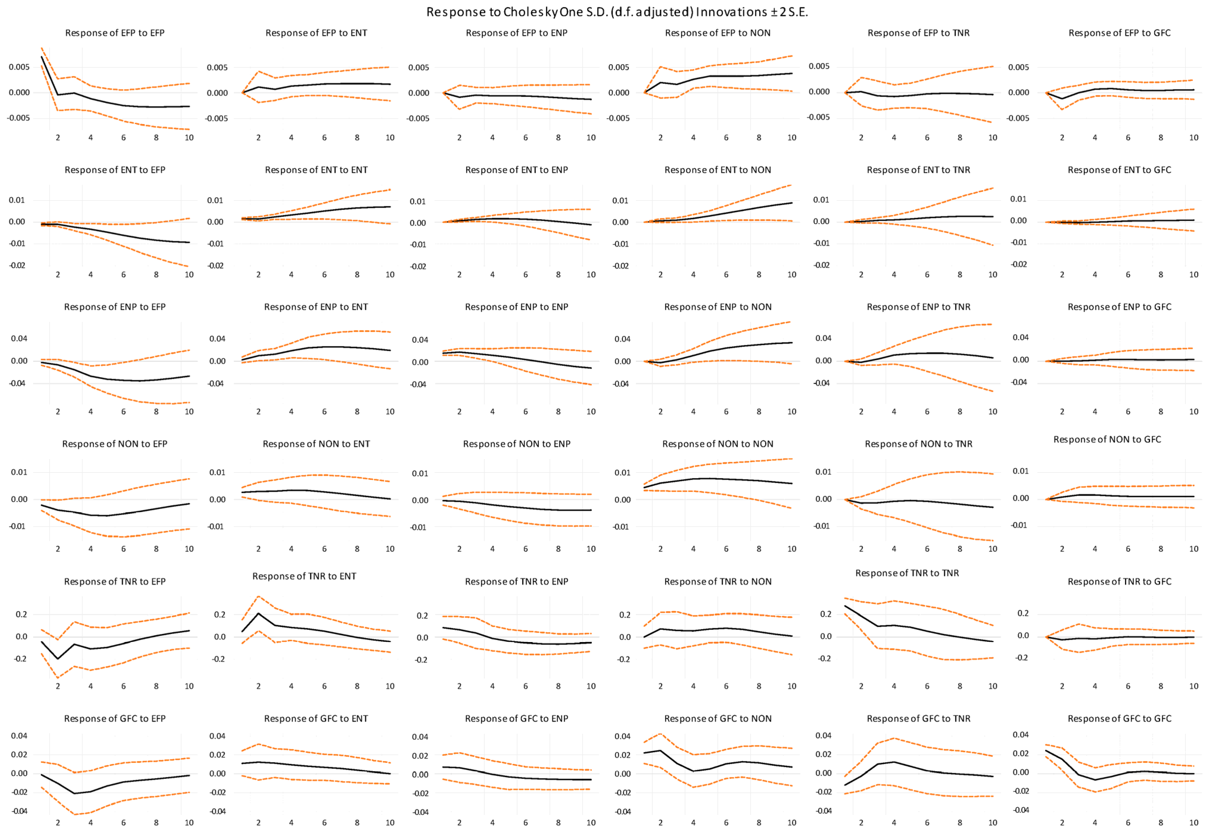
In the framework of the time-series analysis, especially in the VAR models, the impulse response function (IRF) plays an important role. This work aims to compare the effect of a small change or a shock in one variable in a system on changes in the other variables over a period. The use of IRFs leads to a direct visualization and analysis of the system’s response amplitude and time; this brings a substantial understanding of the dynamic interactions between the variables in the system. An often-needed and valued application is policy analysis, as well as projecting and understanding the effects of actions or other occurrences on complex procedures. Figure 5 displays the results of IRFs, which reflect the impact of the variables studied in this research.

The IRF is a widely used method in the econometric literature for analyzing the time evolution of a variable after a shock in another variable by holding all other variables constant. A shock is generally regarded as adding or subtracting one standard deviation from the impulse variable. The IRF declares that a small change in ENT, ENP, NON, TNR, and GPC will positively influence the ecological footprint, indicating that a small change in predictors has a significant influence on the ecological footprint.

The response points to the ways in which different variables move with regard to this shock over a particular time frame. The IRF provides insight into the influence of a shock on variables at various time delays, enabling the observation of the evolving effects of the shock. The numerical values in the IRF serve as an indicator of the magnitude of the response, with larger values suggesting a more significant size of the reaction. Additionally, the signs of the values within the IRF provide information regarding the direction of the response. Confidence intervals, commonly depicted as blue regions in an IRF plot, serve the purpose of assessing the statistical significance of the deviation of the IRF from a null value of zero. Furthermore, the beauty of the IRF is that it spotlights the fluctuation in dependent and independent factors simultaneously. It shows that a change in energy transition and energy-related patents significantly decelerates the adverse effects on the environment while the implications of non-renewable energy and natural resource utilization escalate the environmental change. In contrast, a change in ENT will promote EPTs, encourage the responsible utilization of natural resources, and decelerate the implications of non-renewable energy.

The cumulative impact on each independent component is shown in Figure 6, which also takes into consideration the dependent variable. It is shown in Figure 6 that if we make use of all of our independent components effectively and efficiently, we will be able to reduce our carbon emissions via efficient implementation of the energy transition, energy patents, efficient utilization of natural resources, and gross capital development, which will reduce the dependence on renewable or environmentally friendly sources of energy generation.

Discussion

The stationarity test was employed on a time-series framework to uncover the stationarity statuses of EFP, ENT, ENP, NON, TNR, and GFC and to establish the appropriate lag order for the model, as well as to investigate the cointegration with regime changes and to identify the dynamic interdependencies of various variables. Here are some of this study’s most important conclusions: For all six variables, we rejected the null hypothesis of the Lee–Strazicich unit root test, which confirms the necessity of accounting for structural shifts when modeling time series. The test results were far below the threshold values for many levels of significance for non-stationarity. Further decomposition of the LLC of our modeling showed that lag 4 adequately balanced an even order and over-parametrization, meaning it was the most suitable.

The Gregory–Hansen test for cointegration with regime shifts was used to measure the long-term relationships between variables and show the existence of significant shifts at specific points in time. Longitudinal relationships were also discovered by the ARDL model, revealing that lag 4 seems to be preferable for modeling. The internal validity and reliability of this study were confirmed by diagnostic checks, which showed that the models aligned with the fundamental statistical assumptions. The VAR model has the capability of fitting a long-horizon VAR equation and showing the response of the system if one variable is changed for, say, 10 years, and for how many years the effects of the change will still be felt in the system. Variations in the impulse responses due to external disturbances were effectively captured by the IRF analysis, thus giving us an understanding of the system’s behavior.

The following are the major implications of the results of this study. In the first instance, the imperative of accounting for structural change as a critical factor in any method of analysis or projection is underscored by the observation of structural shifts and non-stationarity in the time-series data used in this research. If not accounting for structural change, Widman and Hua’s findings are cross-sectional instead of developmental, which, in turn, entails erroneous deductions and forecasts. In order to obtain a good forecast accuracy and, at the same time, a rational use of resources, it is crucial to find a good working balance between the complexity and accuracy of the models, as can be seen from the LLC analysis determining the proper lag order. The extent of co-movement amongst variables with an exchange in regimes is discovered and proven through cointegration. This has profound implications in fields such as economics and finance, which require information on how dependencies change over time for decision-making to be informed. This study’s results are in line with those of previous studies [72,73,74].

Conclusions made using the ARDL model are regarded as balanced and consider both short-term and long-term relations between variables and systems’ dynamics. An improved prediction and policy analysis are facilitated by the adoption of the VAR model and IRF analysis, which indicates how changes in some variables impact the rest of the system. These findings are similar to that of the previous study conducted by Tufail et al. [75]. We are equally aware of the fact that while analyzing cointegration, issues such as structural breaks, lag order, and dynamics should not be ignored. The results conform with two earlier studies [76,77] approving the application of VAR models for dynamic interdependency analysis and highlighting the requirement of comprehensive model diagnoses.

In regard to our hypothesis about the significant influence on environmental impact, ARDL validates that the energy shift significantly influences China’s ecological scenario, while new energy generation sources negatively impact climate change. Although the reckless utilization of natural resources predominantly impacts the environment negatively, non-renewable energy, on the contrary, significantly positively affects the environment in China. Consequently, it may be reported that the energy shift and energy-related patents significantly lower the catastrophic environmental impact, while the lesser utilization of natural resources and non-renewable energy significantly positively fosters environmental change.

Although the findings hold up to a battery of statistical tests, it is important to remember that they are only one possible interpretation. There may be unobserved factors impacting the variables, and findings from alternative models or methods might differ slightly. Furthermore, there were restrictions to this study. Alternative approaches were not thoroughly investigated, leaving us uncertain whether the chosen models and criteria are adequate for the data. In addition, the outcomes may only apply to the given dataset and not any others.

In the future, further research could be performed on other variables, or the model could be tested with other forms of time-series modeling or in sample checks with different datasets. Decision-makers may also wish to conduct more studies on the economic or ecological impact of the discovered relations.

This study contributes to the literature on time-series analysis by presenting a comprehensive discussion on structural abnormalities, the choice of lag order, cointegration with a regime shift, and dynamic relationships among the variables. Concerning these results, conclusions may be made, for example, concerning the possibility of forecasting essential parameters, making choices, and understanding the temporal changes in constructions that belong to complex systems.

5. Conclusions

The objective of this study was to provide detailed information on the time-series analysis methods that have been used in the empirical analysis of the variables EFP, ENT, ENP, NON, TNR, and GFC. Thus, the key objectives of this study were to identify the specifics of stationarity, to determine the lag orders, to establish the cointegration with regime shifts, and to discover the dynamic interactions between these variables. During our work, we gained some important insights: Chiefly, as we observed structural breaks and non-stationary data, we stress the importance of taking structural change into account in any analysis.

Regarding the lag length criterion, in our analysis, we found lag 4 to be the optimum for the modeling since this option has the best fit between the model’s complexity and accuracy. The Gregory–Hansen test gave information regarding cointegration with the switchover in regime assumption, allowing for an understanding of constant change in the connection position in the process. A vivid and dynamic description of the system’s characteristics was produced with the ARDL model, which allowed for the consideration of short-term and long-term dependencies between variables. Moreover, the reliability of the developed models was confirmed by diagnostic testing.

In a world that is characterized by ongoing change and uncertainty, the information that we obtained from our research enables us to make more well-informed decisions. It serves as a timely reminder that to thrive in the face of ever-shifting circumstances, we need to be resilient, flexible, and forward-thinking. Let us take the insights gained from this study and use them as we move forward in areas such as economics, finance, environmental policy, and other fields. Let us make our choices based on the evidence, encourage collaboration among different fields of study, and be ready to adjust to the ever-shifting environment.

In conclusion, the insights that were acquired from this study are not the end but rather the beginning; they provide a foundation upon which we may develop solutions that are more resilient and effective for the difficulties that are still to come. Let us move forward with self-assurance, secure in the knowledge that gaining an awareness of the fluidity that characterizes our environment will ultimately lead to a future that is brighter and more stable.

Energy transitions and EPTs provide the basis of the European Union’s sustainability strategy, which was the primary subject of the present study. In addition, this study explored how economic growth, non-RE resources, natural resources, and gross fixed capital contribute to the justification of EFP patterns. Moreover, this research investigated the variables’ stationarity, heterogeneity in slope coefficients, and cross-sectional dependence. In cases where the slope coefficients varied, it was proven that certain EU nations are dependent on one another. Panel cointegration was further applied when the variables became stationary. Following that, CS-ARDL provided both short-term and long-term justification for the outcomes.

According to the results, China’s environmental impact can be reduced through energy transition and patents. Conversely, there is a pressing need to transform economic expansion and resource use into more sustainable management techniques in order to address the environmental impairments caused by non-RE, natural resources, and economic growth. Gross fixed capital formation leads to increased EFP, which is a kind of natural instability that goes against many previous conclusions. Although the directions of the magnitude of the coefficients vary, the arguments were verified using AMG and CCEMG calculations. This study’s empirical findings have real-world policy implications, particularly in the Chinese setting:

• It is recommended that in order to further the clean energy transition, China should tackle the powerful and pervasive obstacles to such activities. The transition to a low-carbon economy is a globally shared goal, and China should do its part to facilitate the export of technology known for its energy efficiency. Moreover, as an alternative to relying on fossil fuels, we may promote the energy transition by raising public awareness of environmental issues and the importance of finding sustainable energy sources.
• Energy patents, as a method of technical progress, are also seen as a great way to lessen the impact on the environment, similar to reducing the EFP. Consequently, the European Union is strongly encouraged to make strategic investments in green patent research and development. Reducing the reliance on non-renewable sources is only one of advantages that might accrue from such coordinated efforts. Furthermore, the technological acceptance model holds that the European Union area should use the information from this study for ongoing energy-saving research and development.
• The beneficial impact of natural resources on the EFP raises concerns about environmental deterioration; however, improving the management of these resources via the use of efficient human capital and technology might require long-term solutions. At the same time, another productive action would be to diversify economic activity away from reliance on natural resource revenues and toward sustainable development.
• Since the EFP is increasing as a result of economic expansion, China needs to incorporate more environmentally friendly and sustainable practices into its current growth models. Another way to protect from environmental pollution is for various companies to switch to green energy gradually. These industries have a significant impact on the production and consumption of many products and services.

We end by emphasizing several limits and potential directions. For instance, this study’s narrow focus on China means that the regional implications for SDG-related strategic strategies are uncertain. When it comes to defining the sustainability agenda, this study also disregards the importance of human capital, individual indicators of energy transition, green investment, financial inclusion, and development. To produce fresh empirical results and policy recommendations, future research should lift these constraints. For future cross-sectional comparisons and improved policy suggestions, it would be helpful to divide EU states into highly polluted and less polluted categories according to the EFP or carbon emissions.