Economic and Technical Aspects of Power Grids with Electric Vehicle Charge Stations, Sustainable Energies, and Compensators

Abstract

The study applies the black kite algorithm (BKA), equilibrium optimizer (EO), and secretary bird optimization algorithm (SBOA) to optimize the placement of electric vehicle charge stations (EVCSs), wind turbine stations (WTSs), photovoltaic units (PVUs), and capacitor banks (CAPBs) in the IEEE 69-node distribution power grid. Three single objectives, including power loss minimization, grid power minimization, and total voltage deviation improvement, are considered. For each objective function, five scenarios are simulated under one single operation hour, including (1) place-only EVCSs; (2) place EVCSs and PVUs; (3) place EVCSs, PVUs, and CAPBs; (4) EVCSs and WTSs; and (5) EVCSs, PVUs, WTSs, and CAPBs. The results indicate that the EO can find the best solutions for the five scenarios. The results indicate that the EO and SBOA are the two powerful algorithms that can find optimal solutions for simulation cases. For one operating day, the total grid energy that is supplied to base loads and charge stations is 80,153.1 kWh, and many nodes at high load factors violate the lower limit of 0.95 pu. As for installing more renewable power sources, the energy that the base loads and charge stations need to supply from the grid is 39,713.4 kWh. As more capacitor banks are installed, the energy demand continues to be reduced to 39,578.9 kWh. The energy reduction is greater than 50% of the demand of all base loads and charge stations. Furthermore, the voltage can be significantly improved up to higher than 0.95 pu, and a few nodes at a few hours fall into the lowest range. Thus, the study concludes that the economic and technical aspects can be guaranteed for DPGs with additional installation of EVCSs.

1. Introduction

1.1. The Motivation

The world is facing the urgent issue of global warming [1] and climate change [2], primarily due to the increase in CO₂ emissions [3]. To deal with such situations and mitigate the adverse effects, the need for international agreements or treaties is urgent, and the Paris Agreement is one of the solutions that has been highly accepted and joined by many countries [4]. The agreement seeks to unite global efforts by setting clear targets to mitigate the most severe consequences of climate change, ensuring a sustainable future. The goal is essential to mitigating the most severe consequences of climate change.

Countries are also implementing strategies to mitigate the effects, such as transitioning to electric vehicles (EVs) [5]. A study in China [6] used the Gaussian two-step floating catchment area (G2SFCA) method to evaluate the spatial accessibility of public electric vehicle charging stations (EVCSs). The results revealed an uneven distribution of EV infrastructure across the country, emphasizing the need for robust policy support and technological advancements to promote EV adoption and sustainability. Similarly, a study examining Istanbul [7] utilized a three-step approach to evaluate optimal EVCS locations based on various geospatial criteria. The findings indicated that the most suitable areas for EVCS placement in Istanbul are concentrated in the southeastern part of the European side and the southwestern portion of the Anatolian side.

1.2. The Development Statuses of EVCSs to Serve EV Growth in Several Countries and Territories

In [8], the authors in the study emphasize the critical need for expanding EVCS infrastructure in the U.S. and also highlight the importance of having a proper strategy for placing and developing EVCSs in residential areas to enhance EV growth. In addition, the study also suggests a framework for optimal placement to support businesses and underlines the significance of choosing the right charger type and location and considering consumer needs for the success of EVCS projects. Next, the author in [9] explores the financial aspects of establishing public charging stations (PCSs) in rural U.K. areas, using linear programming to forecast EV adoption and financial returns. Despite finding most rural PCSs unprofitable in the long term, the author proposes different solutions, such as reducing the number of chargers per station and adjusting electricity prices to enhance viability, calling for investment based on these strategies. In [10], the authors evaluate the feasibility of placing EVCSs in different cities and towns in Sri Lanka, considering various aspects, and finally conclude that public hotspot-based EVCSs are feasible and highly suggest the implementation. At the same time, environmental benefits and market potential are also considered.

1.3. The Literature Review About the Integration of the ECVS Distribution Power Grid

In [11], a fuzzy multi-objective model employing a genetic algorithm (GA) is introduced for the optimal placement and sizing of EV charging stations (EVCSs), aiming to improve traffic flow and reduce power loss within both transportation and power distribution networks. This model takes into account variables like traffic density and existing power infrastructure, demonstrating its efficacy through a case study involving a 33-node power grid and a 25-node traffic network. In [12], the author emphasizes the need for an expanded charging infrastructure due to the growing number of electric vehicles (EVs), then a scenario analysis framework for Beijing’s Changping district is proposed; the scenario provides a capability to estimate the need for advanced charging technologies by 2020. In [13], the hybrid AGWOPSO algorithm is presented, outperforming traditional GWO and PSO algorithms in optimizing EVCS and capacitor placement on IEEE 33-node and 34-node distribution power grids (DPGs), enhancing grid performance and profitability. The authors in [14] develop and evaluate a mathematical model using the modified primal-dual interior point algorithm (MPDIPA) to optimize the size and location of EVCSs on the IEEE 123-node DPG, focusing on minimizing costs and improving power efficiency. Finally, the author in [15] discusses the impact of imprecisely placed level 3 EVCSs on the stability of electric distribution power grids (EDPGs), proposing the use of particle swarm optimization (PSO) to find optimal placements of EVCSs and photovoltaic units (PVUs) on a 52-node EDPG for cost minimization and system load balancing. The Jaya algorithm has shown a significant improvement over existing techniques by optimizing voltage, cost, and power loss [16]. The Balanced Mayfly Algorithm (BMA) was applied to find a better size and location of EVCSs in Allahabad, India, than particle swarm optimization variants [17]. The study in [18] proposed a stochastic model that integrates EVCSs with wind energy to enhance the efficiency of multi-level charging infrastructures, energy storage, and network reinforcement, effectively reducing energy and infrastructure costs while maintaining system balance. In [19], the use of HOMER software for real-world data analysis reveals that in addition to the many environmental benefits provided by renewable energy sources, the combined systems incorporating diesel, photovoltaics, and battery storage are more cost-effective for both isolated and connected EVCS models. Battery energy storage systems were considered in power grids with the operation of EVCSs under the consideration of land limits [20]. The integration of demand response strategies, photovoltaic units, and energy storage systems into residential EVCSs, considering the challenges caused by PVU output uncertainties and load demand variation, was concerned with using the fuzzy logic approach in [21] and a hybrid optimization method in [22]. The challenges and opportunities of integrating EVCSs from the perspectives of different stakeholders and the impacts on distribution networks were discussed in [23]. The study in [24] introduced a novel strategy for improving radial DPG performance through optimal placement of DGs, DSTATCOMs, and EVCSs using a new algorithm, significantly reducing power loss and enhancing voltage stability. In [25,26], the authors evaluated the impact of integrating EVCSs into DPGs, focusing on grid stability. The solar–biogas EVCSs for cost-effective charging in Bangladesh were optimally placed [27]. Voltage stability in the Indian grid was proved by integrating DSTATCOM and using the Bald Eagle Search Algorithm (BESA) [28]. Furthermore, the authors in [29] optimize the placement of both RES and fast charging stations (FCSs) using the red kite optimization algorithm (ROA) to minimize power loss and voltage issues in IEEE 33- and 69-node DPG configuration. In conclusion, ROA has proven itself to reach a high level of computational performance and reliability while the scale of the considered problem has become larger. The study in [30] focused on the optimization of EV types, battery energy storage systems (BESSs), and charging methods. In addition to EVCSs, BESSs have also been considered to be placed in different configurations of DPGs [31], recently as auxiliary devices to improve the stability and reliability of the whole grid. Due to their function, which can charge or discharge the power as controlled, BESSs are also used as a solution to mitigate the negative effects caused by EVCSs on the grid [32]. However, the combination of EVCS, BESSs, and all other auxiliary devices must be strictly evaluated and assessed in the planning process as executed in [33]. To support the planning process mentioned in [33], the authors in [34] applied an optimal algorithm called the multi-objective thermal exchange optimization algorithm (MOTEO) to determine the best placement of both EVCSs and BESSs. In [35], a two-stage stochastic programming approach was used to optimize the energy procurement and equipment dispatch of an electric vehicle charging station (EVCS). Next, the application of a recently proposed optimization called the Honey Badger Algorithm (HBA) is conducted to accommodate BESSs and wind turbines (WTs) along with an EVCS in the IEEE-69 node DPG [36]. Furthermore, the authors in [37] issued several challenges faced by electric vehicle (EV) charging networks, such as power losses and high energy costs. A hybrid approach combining War Strategy Optimization (WSO) and a Radial Basis Function Neural Network (RBFNN) is proposed to mitigate these issues.

1.4. The Novelty and Contribution

In this research, EVCSs, PVUs, CAPBs, and WTSs are considered to optimize their placement in the IEEE 69-node DPG to achieve the minimization of active power loss (OAPL), grid power required at slack node (PSL), and the total voltage deviation (TVD). The black-winged kite algorithm (BKA) [38], equilibrium optimizer (EO) [39], and secretary bird optimization algorithm (SBOA) [40] are applied to determine the optimal placement of EVCSs, PVUs, CAPBs, and WTSs. The main novelties can be summarized as follows.

-

Successfully applied novel metaheuristic algorithms, including the black-winged kite algorithm (BKA) and secretary bird optimization algorithm (SBOA), to optimize the placement of an EVCS in the IEEE 69-node DPG. Both the BKA and SBOA have proven their capability in the development phase compared to other previous methods, including the most iconic ones, such as PSO, DE, or GWO. Regarding the SBOA, personally, the method is superior to most of the recent recently developed ones, such as the nutcracker optimization algorithm (NOA) and Rime optimization algorithm (RIME), which were developed in 2023; golden jackal optimization (GJO)—2022; artificial gorilla troops optimizer (GTO)—2021; etc. Regarding the BKA, the algorithm also outperforms a wide range of state-of-the-art metaheuristic algorithms such as the improved moth flame optimization algorithm (IMFA) and sand cat swarm optimization (SCOA), developed in 2023; golden jackal optimization (GJO) and coati optimization algorithm (COA)—2022; hunter–prey optimization (HPO) and quantum-based avian navigation optimizer algorithm (QANAO)—2021; etc.

-

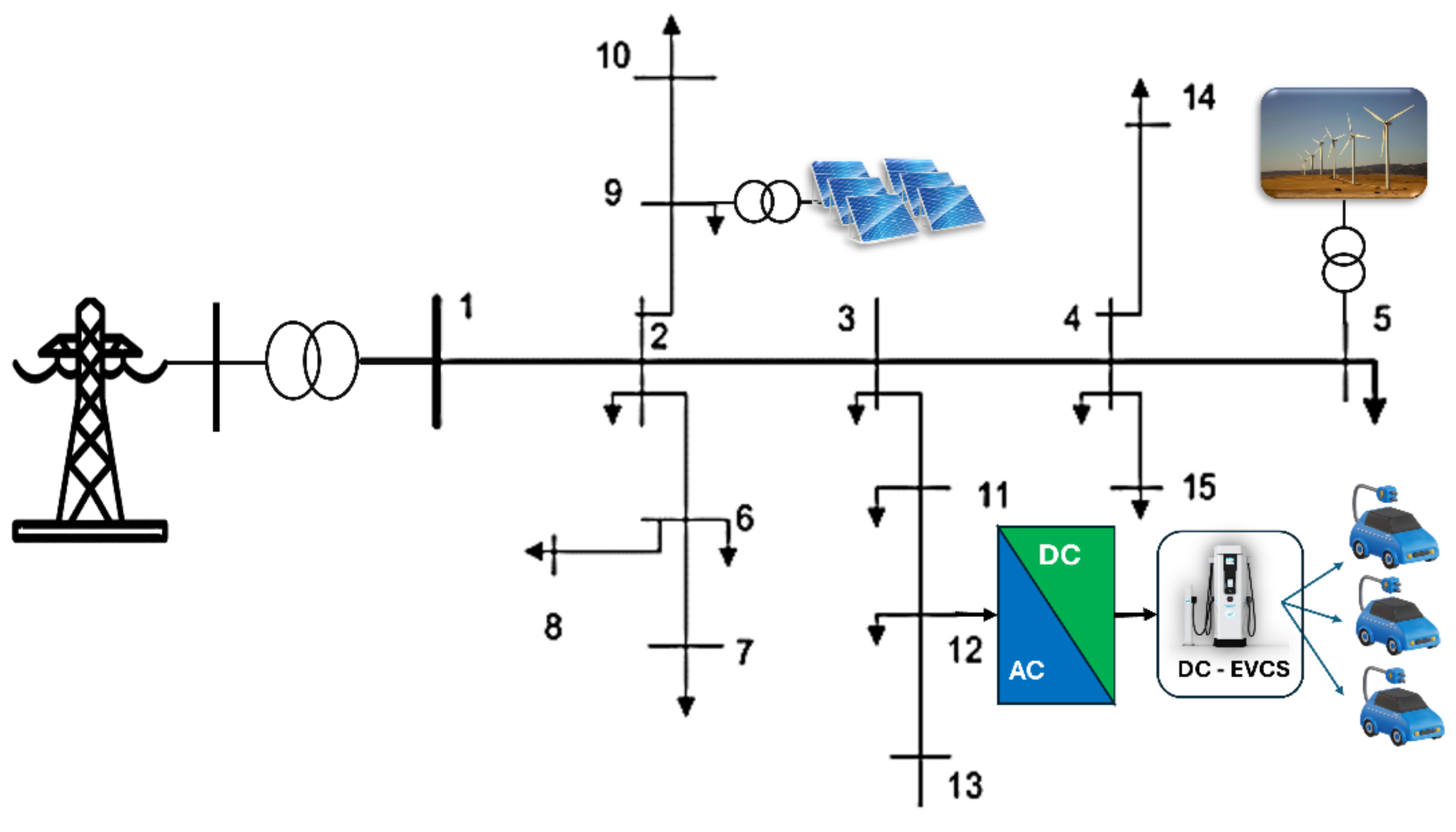
Implemented the integration of ECVSs in three different objective functions with five distinctive scenarios for each considered objective function. For each objective function, the placement of EVCSs is executed along with a particular type of auxiliary devices, which could be CAPBs, PVUs, WTs, or combined with all the mentioned devices to offer a detailed look at the real effectiveness of all these implementations. Based on that, the present valuable references are for the planners, dispatchers, and also operators.

-

As well as providing a detailed look while solving the considered problem on the aspects of planning and designing through different scenarios, as mentioned above, the study also presented the results of solving the problem based on the viewpoint of operational aspects with real data of load demand variation and supplied power form PVU and WT within 24 h.

The main contributions of the research can be summarized as follows:

-

Determine the best-applied algorithm among the three ones using different criteria and specific comparisons.

-

The placement of EVCSs is considered to reach the optimal value of different objective functions, including minimizing the overall active power loss, minimizing the power source at the slack bus, and minimizing the total voltage deviation index.

-

Clarify the effectiveness of placing EVCSs with other auxiliary devices using particular scenarios for each considered objective function and indicate the best scenario resulting in the best value for each considered objective function.

-

Present and analyze in detail the differences in results reached by three objective functions while compared to others, offering a valuable reference for those, especially operators, in terms of optimizing their own DPGs to reach the desired expectations.

-

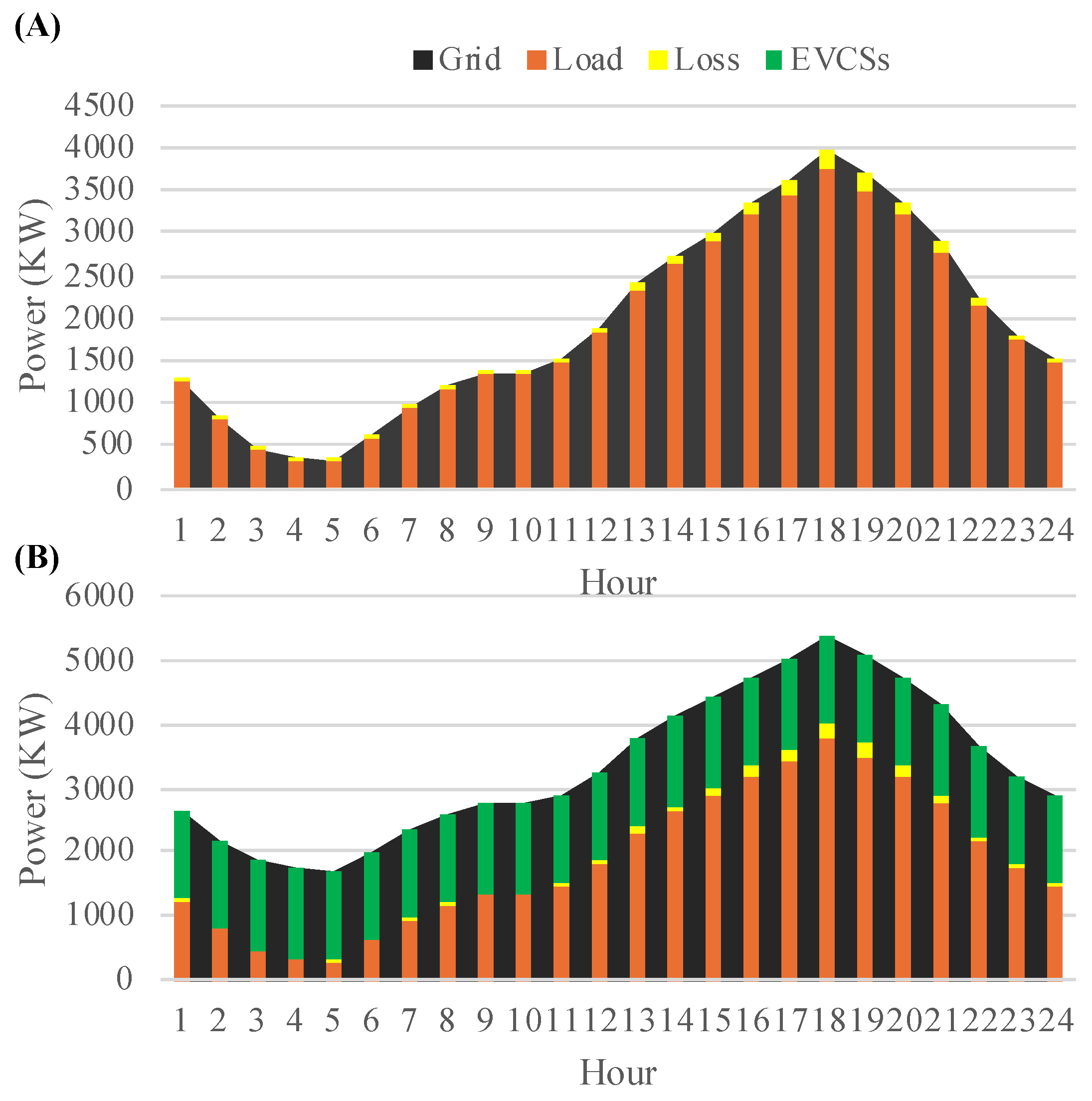
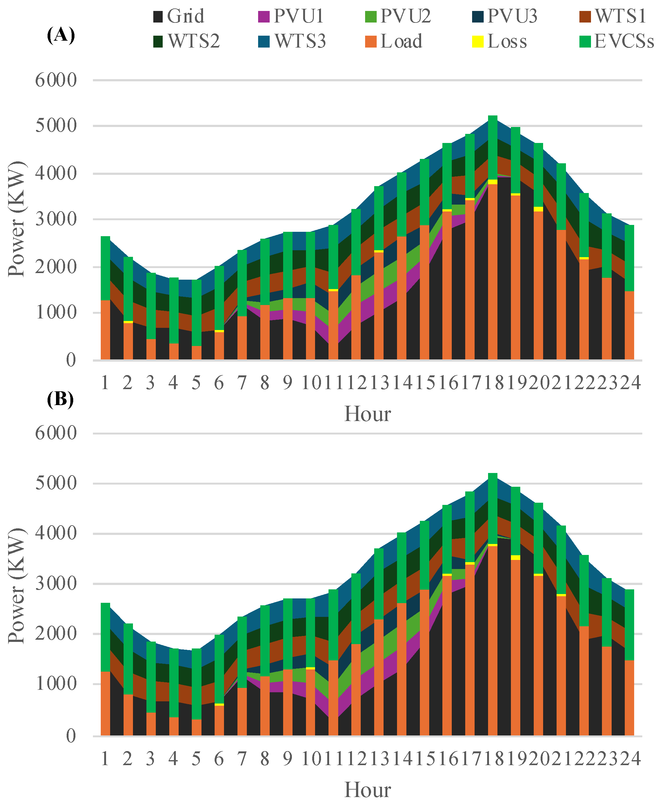
Clarify the contribution of renewable-based distributed generators to the reduction in grid power and present a detailed evaluation using quantitative results while solving the problem considered from an operational viewpoint.

-

Using particular case studies to demonstrate the effectiveness of utilizing optimization algorithms to solve the considered problem from both the planning and operational viewpoints.

Besides the introduction, the other contents of the research are structured as follows: Section 2 will present the main objective functions and the involved constraints; Section 3 briefly describes the applied methods focused on their distinctive features; Section 4 presents the results and related detailed analysis regarding the actual effectiveness of the applied methods and different employments of the considered problem; lastly, Section 5 reveals the essential conclusions of the whole research, and the downsides and the future orientation of the research are also mentioned.

2. Problem Formulation

In this study, distribution power grids with the operation of electric vehicle charge stations and renewable power sources were optimally operated over one day to reduce total energy loss and grid energy and improve voltage profile. A typical structure of the integrated distribution power grid is plotted in Figure 1.

2.1. The Main Objective Functions

• Reduction of overall active power loss: Total active power loss (PLoss_all) is caused due to the flow of electric current in the distribution lines (branches). Hence, the more branches the given grid has, the larger PLoss_all is; therefore, reducing PLoss_all is really important. The mathematical expression of PLoss_all is formulated as follows:

$$Reduce {PLoss}_{all}=\sum _{bra=1}^{N_{bra}}(3\times I_{bra}^2\times R_{bra})$$

(1)

where ${PLoss}_{all}$ is the overall active power loss; $I_{bra}$ is the current amplitude on the brath branch; $N_{bra}$ is the total number of branches; and $R_{bra}$ is the resistance of the branch bra.

• Reduction in grid power consumption: Grid power is supplied to loads by the transformer at the slack node. So, the second objective is to reduce the total grid power as shown in the following expression.

$$\begin{gathered} Reduce P_{grid}=\sum _{n=2}^{N_{nd}}{P}_{DM,n}+\sum _{j=1}^{N_{LV1}}{P}_{LV1,j}+ \\ \sum _{k=1}^{N_{LV2}}{P}_{LV2,k}+\sum _{l=1}^{N_{LV3}}{P}_{LV3,l}+{PLoss}_{all}-\sum _{w=1}^{N_{WT}}{P}_{WT,w}-\sum _{s=1}^{N_{PVU}}{P}_{PVU,s} \end{gathered}$$

(2)

where $P_{grid}$ is the active grid power at the slack node supplied by the transformer; $\sum _{n=2}^{N_{nd}}{P}_{DM,n}$ is the total active power of loads at from nodes 2 to node $N_{nd}$ and $N_{nd}$ is the number of nodes; $\sum _{j=1}^{N_{LV1}}{P}_{LV1,j}$ is the power demanded by all EVCS level 1, with j = 1, 2, …, $N_{LV1}$ and $N_{LV1}$ is the number of Level 1 EVCSs; $\sum _{k=1}^{N_{LV2}}{P}_{LV2,k}$ is the power demanded by all Level 2 EVCS, with k = 1, 2, …, $N_{LV2}$ and $N_{LV2}$ is the number of Level 2 EVCSs; $\sum _{l=1}^{N_{LV3}}{P}_{LV2,l}$ is the power demanded by all Level 3 EVCSs, with l = 1, 2, …, $N_{LV3}$ and $N_{LV3}$ is the number of Level 3 EVCSs; $\sum _{w=1}^{N_{WTs}}{P}_{WT,w}$ is the total active power supplied by all installed WTSs; $\sum _{s=1}^{N_{PVU}}{P}_{PVU,s}$ is the total active power supplied by all installed PVUs; and $N_{WT}$ and $N_{PVU}$ are, respectively, the number of installed WTSs and PVUs.

• Reduction in total voltage deviation (TVD): The deviation between nominal and real voltages reflects the voltage stability of the system. So, minimizing the TVD of the given grid is also crucial, as modeled by the following objective function [41]:

$$Minimize TVD=\sum _{n=1}^{N_{nd}}\left|1-V_n\right|$$

(3)

where $V_n$ is the voltage magnitude at node n.

2.2. The Involved Constraints

• Power balance constraints: The most important condition for a stable operation of distribution systems is the balance of power between consumption and supply. The constraints are expressed as follows:

$$\begin{gathered} \sum _{n=2}^{N_{nd}}{P}_{DM,n}+\sum _{j=1}^{N_{LV1}}{P}_{LV1,j}+ \\ \sum _{k=1}^{N_{LV2}}{P}_{LV2,k}+\sum _{l=1}^{N_{LV3}}{P}_{LV3,l}+{PLoss}_{all}-\sum _{w=1}^{N_{WT}}{P}_{WT,s}-\sum _{s=1}^{N_{PVU}}{P}_{PVU,s}-P_{grid}=0 \end{gathered}$$

(4)

$$P_{grid}+\sum _{w=1}^{N_{WT}}{P}_{WT,w}+\sum _{s=1}^{N_{PVU}}{P}_{PVU,s}=\sum _{n=2}^{N_{nd}}{P}_{DM,n}+\sum _{j=1}^{N_{LV1}}{P}_{LV1,j}+\sum _{k=1}^{N_{LV2}}{P}_{LV2,k}+\sum _{l=1}^{N_{LV3}}{P}_{LV3,l}+{PLoss}_{all}$$

(5)

$$Q_{grid}+\sum _{c=1}^{N_{CAPB}}{Q}_{CAPB,c}+\sum _{w=1}^{N_{WTs}}{Q}_{WT,w}=\sum _{n=2}^{N_{nd}}{Q}_{DM,n}+\sum _{bra=1}^{N_{bra}}(3\times I_{bra}^2\times X_{bra})$$

(6)

where $Q_{grid}$ is the reactive power supplied by the sole transformer at the slack node or from the transmission grid; $\sum _{c=1}^{N_{CAPB}}{Q}_{CAPB,c}$ is the total amount of active power injected to the grid by all capacitor banks with c = 1, 2, …, $N_{CAPB}$ and $N_{CAPB}$ is the number of capacitor banks placed in the grid; $\sum _{w=1}^{N_{WT}}{Q}_{WT,w}$ is the total reactive power supplied by all placed WTSs; $\sum _{n=2}^{N_{nd}}{Q}_{DM,n}$ is the total reactive power of load demand at all nodes; and $X_{bra}$ is the reactance of branch bra.

• Operational voltage constraint: Voltage is another critical factor that directly affects the reliability and stability of a particular DPG; therefore, voltage must be maintained in the allowed ranges between the minimum and maximum values as follows:

$$V^{min} \le V_n \le V^{max};n=1, \dots , N_{nd}$$

(7)

where $V^{min}$ and $V^{max}$ are the minimum and maximum values of voltage magnitude for all nodes; and $V_n$ is the operating voltage magnitude at the node n.

• Thermal constraint: This constraint is mainly about the current amplitude circulated through a particular branch. The constraint can be expressed as follows:

$$I_{bra} \le { I}_{bra}^{max}$$

(8)

where ${ I}_{br}^{max}$ is the maximum current amplitude of the branch bra.

• PVU operation constraints: These constraints set the legal ranges to the amount of active power supplied to grid by PVUs. The mathematical expression of the constraint is as follows:

$$\begin{gathered} P_{PVU}^{min} \le P_{PVU,s} \le P_{PVU}^{max}; \\ s=1, \dots , N_{PVU} \end{gathered}$$

(9)

where $P_{PVG}^{min}$ and $P_{PVG}^{max}$ are the minimum and maximum active powers supplied by the PVU s.

• CAPB operation constraints: The amount of reactive power supplied by CAPBs can only vary in the allow ranges as follows:

$$\begin{gathered} Q_{CAPB}^{min} \le Q_{CAPB,c} \le Q_{CAPB}^{max}; \\ c=1, \dots , N_{CAPB} \end{gathered}$$

(10)

where $Q_{CAPB}^{min}$ and $Q_{CAPB}^{max}$ are the minimum and maximum reactive powers supplied by the CAPB c.

• WTS operation constraints: WTSs can work safely and efficiently as their designed capability when they are operating within their limits as follows:

$$P_{WT}^{min} \le P_{WT,w} \le P_{WT}^{max};w=1, \dots , N_{WT}$$

(11)

$$Q_{WT}^{min} \le Q_{WT,w} \le Q_{WT}^{max};w=1, \dots , N_{WT}$$

(12)

where $P_{WT}^{min}$ and $P_{WT}^{max}$ are the minimum and maximum active powers supplied by the WT w; and $Q_{WT}^{min}$ and $Q_{WT}^{max}$ are the minimum and maximum reactive powers supplied by the WT w.

• The position constraints of PVUs, CAPBs, and WTSs: This constraint means that the placements of PVUs, CAPBs, and WTSs are considered legally only if they are placed from node 2 onward to the DPG as follows:

$$2 \le L_{PVU,s} \le N_{nd}$$

(13)

$$2\le L_{CAPB,c}\le N_{nd}$$

(14)

$$2 \le L_{WT,w} \le N_{nd}$$

(15)

where $L_{PVU,s}$, $L_{CAPB,c}$, and $L_{WT,w}$ are, respectively, the locations of the PVU s, CAPB c, and WT w.

• EVCS site constraints: The placements of EVCSs at all levels are accepted only if they are connected to node 2 onward to the last node on the DPG as follows:

$$2 \le L_{LV1,j},L_{LV2,k} , L_{LV3,l} \le N_{nd}$$

(16)

with

$$L_{LV1,j}\ne L_{LV2,k} \ne L_{LV3,l}$$

(17)

where $L_{LV1,j}$, $L_{LV2,k}$, and $L_{LV3,l}$ are the positions of the jth Level 1, kth Level 2, and lth Level 3 stations.

3. Applying EO to Optimize the Allocation of EVCSs and Other Auxiliary Devices

3.1. The Equilibrium Optimizer (EO)

The EO was developed by Faramarzi et al. in 2020 by inspiring the concept of mass balance in the given control volume [39]. In the optimal process, each solution in the initial population of the EO is characterized by a concentration. The concentration of all solutions is consistently updated until the equilibrium state in the given control volume is established. When the equilibrium state is already found, the optimal concentration is determined [42]. The mathematical model of the update method executed by the EO is presented as follows:

$$E_n^{new}=E_{Top}+\left(E_n-E_{Top}\right)\times EP+{\displaystyle \frac{GR}{RC\times GCV}}\times \left(1-EP\right)$$

(18)

with

$$E_{Top}\in \left[E_{Top1};E_{Top2};E_{Top3};E_{Top4};E_{TopAver} \right]$$

(19)

$$\begin{gathered} EP=2\times \left|RD-0.5\right|\times \left[e^{-GCV}-1\right] \\ with GCV={\left(1-{\displaystyle \frac{It}{{It}^{max}}}\right)}^{1-{\displaystyle \frac{It}{{It}^{max}}}} \end{gathered}$$

(20)

$$GR={\displaystyle \frac{1}{2}}\times EP\times (E_{Top}-GCV\times E_n)$$

(21)

where $E_n^{new}$ is the nth new solution with n = 1, 2, …, N_pz; $E_{Top}$ is selected from the top four best solutions ($E_{Top1};E_{Top2};E_{Top3};E_{Top4}$) and the average top solution, $E_{TopAver}$. $E_{TopAver}$ is the mean solution of ($E_{Top1};E_{Top2};E_{Top3};E_{Top4}$); $E_n$ is the nth current solution; $EP$ is the exponential parameter; $GR$ is the generation ratio; and $RC$ and $GCV$ are, respectively, the return coefficient and the capacity of the given control volume.

3.2. The Selection of Control and Dependent Variables

The problem of optimizing the placement of EVCSs, CAPBs, PVUS, and WTSs in distribution power grids considers the locations and power of these installed devices so that the power loss, grid power, and standard deviation are minimal. So, the task of metaheuristic algorithms is to determine the best location and power of them.

In assumptions, the study considers the following:

• PVUs with a power factor of 1.0.
• WTSs with a power factor between 0.85 and 0.95.
• Placing one Level 1, one Level 2, and one Level 3 EVCS.

Based on the above assumptions, the power required by EVCSs and the power factor of PVUs are no longer control variables, but the power factor of WTSs, the location of EVCSs, CAPBs, WTSs, and PVUs, the reactive power supplied by CAPBs, the active power supplied WTSs and PVUs are control variables. In addition, all the mentioned control variables except for the power factor of WTs are discrete. That means that their legal value must be the positive integer. Particularly, the location of EVCSs, CAPBs, WTs, and PVUs on the grid must be “21, 22, 23, etc.”. Moreover, the power supplied by WTs and PVUs is also the discrete value that will be later mentioned in detail in Section 4. Specifically, the rated power of WTs is limited between 0 and 500 kW with a step of 100 kW. Similarly, PVUs and CAPBs are also treated in the same manner between zero and their rated values.

After the control variables are determined, the forward–backward sweep technique [43] is run to calculate the branch currents and node voltages. The parameters are called dependent variables, and they are checked and set to penalty terms, as shown in Equations (30) and (31) in [44]. Note that the value of all the branch currents and node voltages are continuous due to the attributes of power flow calculation and also to ensure the accuracy of the desired value of the main objective functions considered in this work.

3.3. The Fitness Function

The study considers three single objective functions shown in Equations (1)–(3), so three fitness functions are formed based on each objective function and the penalty terms of currents and voltages. The fitness function is the sum of the objective and penalty terms, as shown in the study [44].

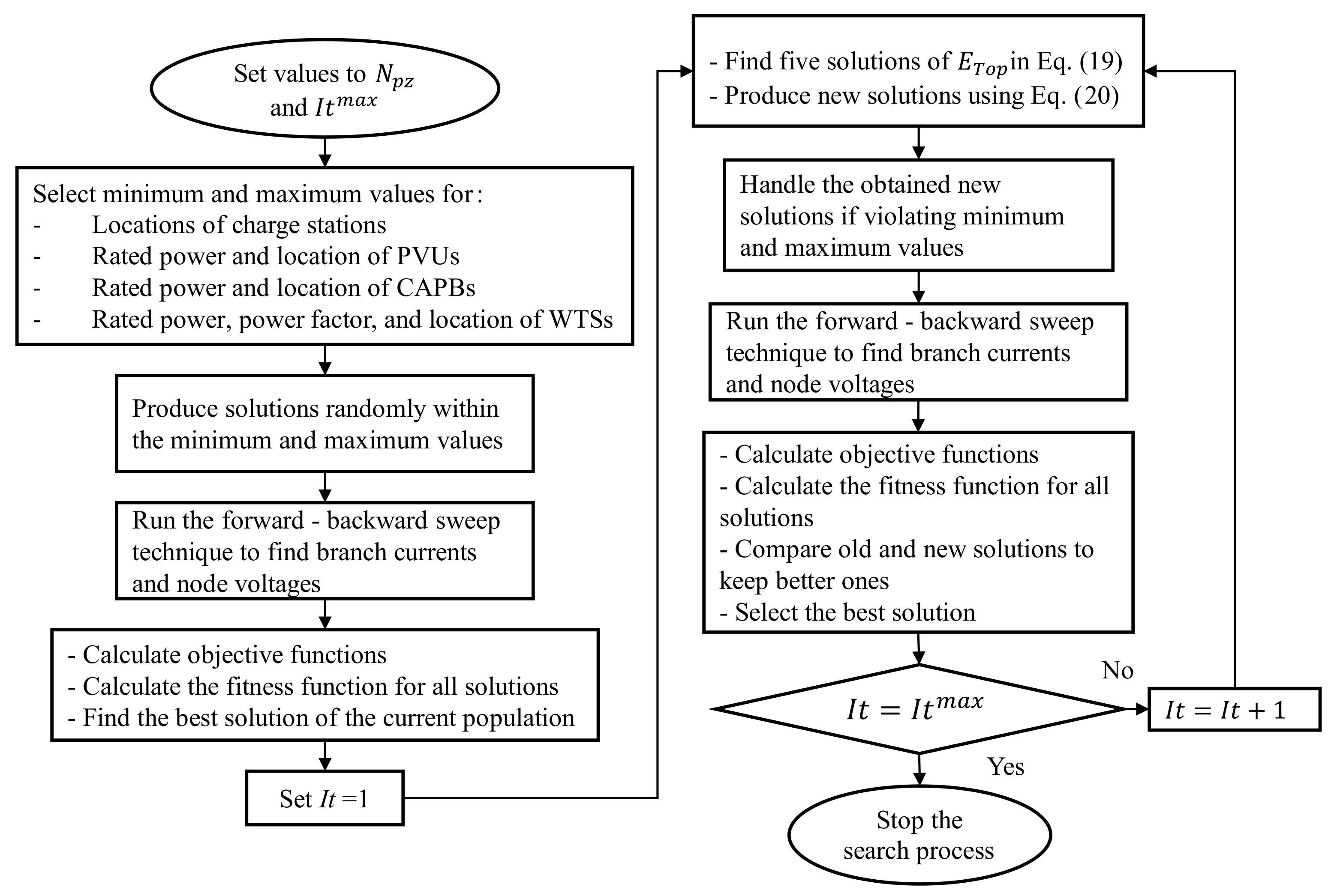
3.4. The Implementation of EO for the Problem

The implementation of the EO for the optimal placement of EVCSSs, CAPBs, PVUs, and WTSs is presented in Figure 2.

4. Results and Discussion

4.1. Simulation Scenarios for the Three Applied Algorithms

In this section, three algorithms, including the BKA, EO, and SBOA, are applied to optimize the placement of EVCSs, CAPBs, WTSs, and PVUs in the IEEE 69-node DPG. The data of the system are shown in [35]. The selected DPG comprises 68 branches, serving a base load demand of 3802.19 kW and 2694.6 kVar. The total active power loss is 225.01 kW, and the grid operates at a nominal voltage of 12.66 kV. For each objective function, four simulation scenarios are summarized in

Table 1. The placement combination of EVCSs and other power sources for four simulation scenarios.

Scenario	PVUs	CAPBs	WTs	EVCSs
1	-	-	-	1 Level 1 station, 1 Level 2 station, and 1 Level 3 station
2	3 PVUs with power factor of 1.0 for each PVU	-	-
3	3 PVUs: power factor of 1.0, 3 kW solar panel	3 CAPBs: 30 kVAr for each step	-
4	-	-	3 WTSs: 100 kW WT and power factor of [0.85, 0.95]
5	3 PVUs: power factor of 1.0, 3 kW solar panel	3 CAPBs: 30 kVAr for each step	3 WTSs: 100 kW WT and power factor of [0.85, 0.95]

. The placement of EVCSs is implemented for all four simulation scenarios with one Level 1 station, one Level 2 station, and one Level 3 station. The details of each level of EVCSs, number of electric vehicles, and total power demand of each station type is given in

Table 2. Summary of electric vehicle charge stations [30].

Type	Rated Power of Each Charger (kW)	Number of Chargers/EVs	Rated Power of Each EVCS (kW)
L1 EVCS	1.9	100	190
L2 EVCS	4.0	50	200
L3 EVCS	100	10	1000

.

Scenario 2 carries out the placement of three PVUs with the power factor of 1.0. It means the PVUs cannot inject reactive power into the grid and the transformer at slack must not supply all reactive power demand to loads. On the contrary, other remaining simulation scenarios consider the reactive power supply from added power sources such as capacitor banks, wind turbines, and photovoltaic units. Scenario 3 carries out the placement of three PVUs with the power factor 1.0 and three other capacitor banks. Scenario 4 places three WTSs, and each WT has a power factor within the range of [0.85; 0.95] [34]. Scenario 5 places three PVUs with the power factor of 1.0, and three CAPBs and three WTSs with power factors between 0.85 and 0.95. The minimum and maximum capacities of each PVU are 0 and 600 kW with a step size of 3 kW. Similarly, the minimum and maximum capacities of the WTSs are 0 and 500 kW with a step size of 100 kW, and the minimum and maximum capacities of the CAPBs are 0 and 600 kVAr with a step size of 30 kVAr. The step sizes of 3 kW of the PVUs, 30 kVAr of the CAPBs, and the 100 kW of the WTs are taken from studies [45,46,47].

This section also discusses and analyzes the actual performance of the three applied algorithms. To reach the best results, we set the control parameters, including the population size (N_pz) and the maximum number of iterations (${It}^{max}$), as shown in

Table 3. Setting control parameters for algorithms for four simulation scenarios.

Scenario	Description	Population	Maximum Iteration Number	Number of Control Variables
Base	Without EVCS and auxiliary devices	-	-	-
1	3 EVCSs	40	200	3
2	3 EVCSs + 3 PVUs	40	500	3 + 6 = 9
3	3 EVCSs + 3 PVUs + 3 CAPBs	100	500	3 + 6 + 6 = 15
4	3 EVCSs + 3 WTSs	100	500	3 + 9 = 12
5	3 EVCSs + 3 PVUs + 3 CAPBs+ 3 WTSs	100	1000	3 + 6 + 6 + 9 = 24

. Moreover, each algorithm executed 50 trials for each scenario. All the results and simulations presented in this research were conducted on a computer with the basic comparisons: a 2.6 GHz central processing unit (CPU) from Intel and 8 GB of random accessing memory (RAM).

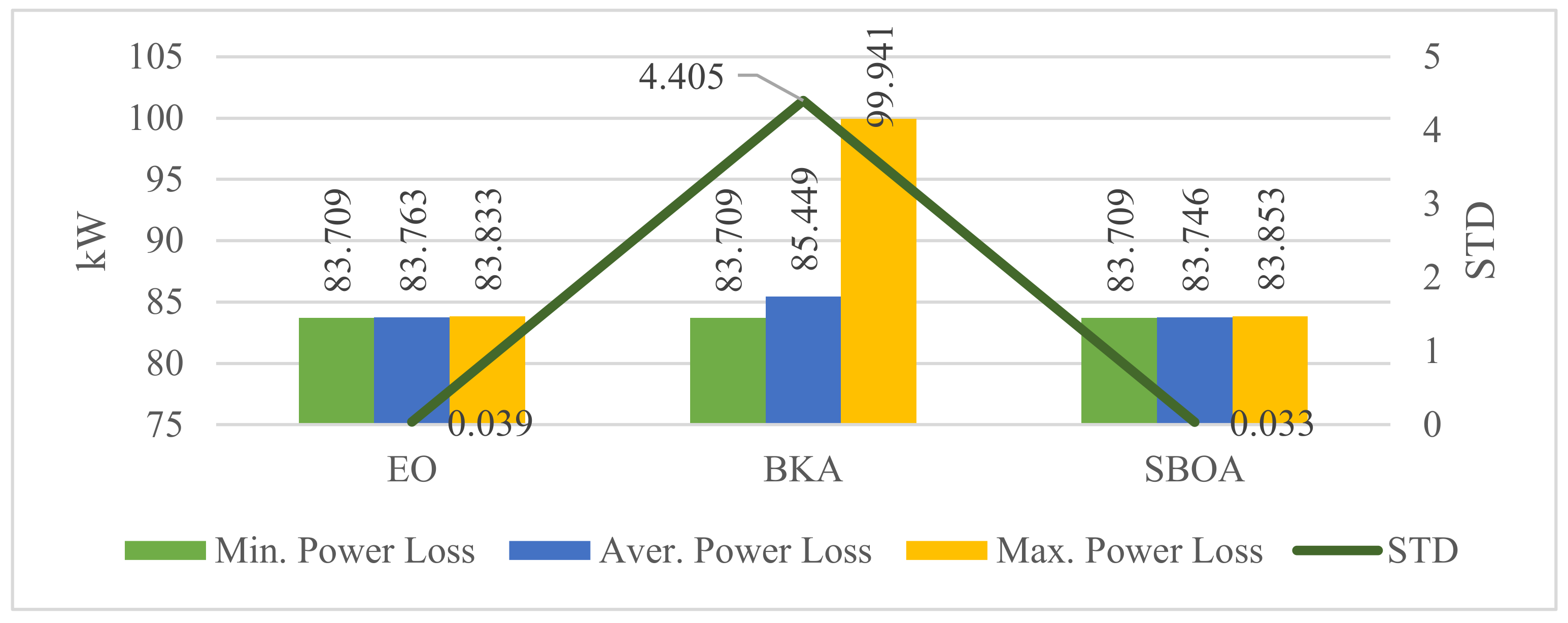
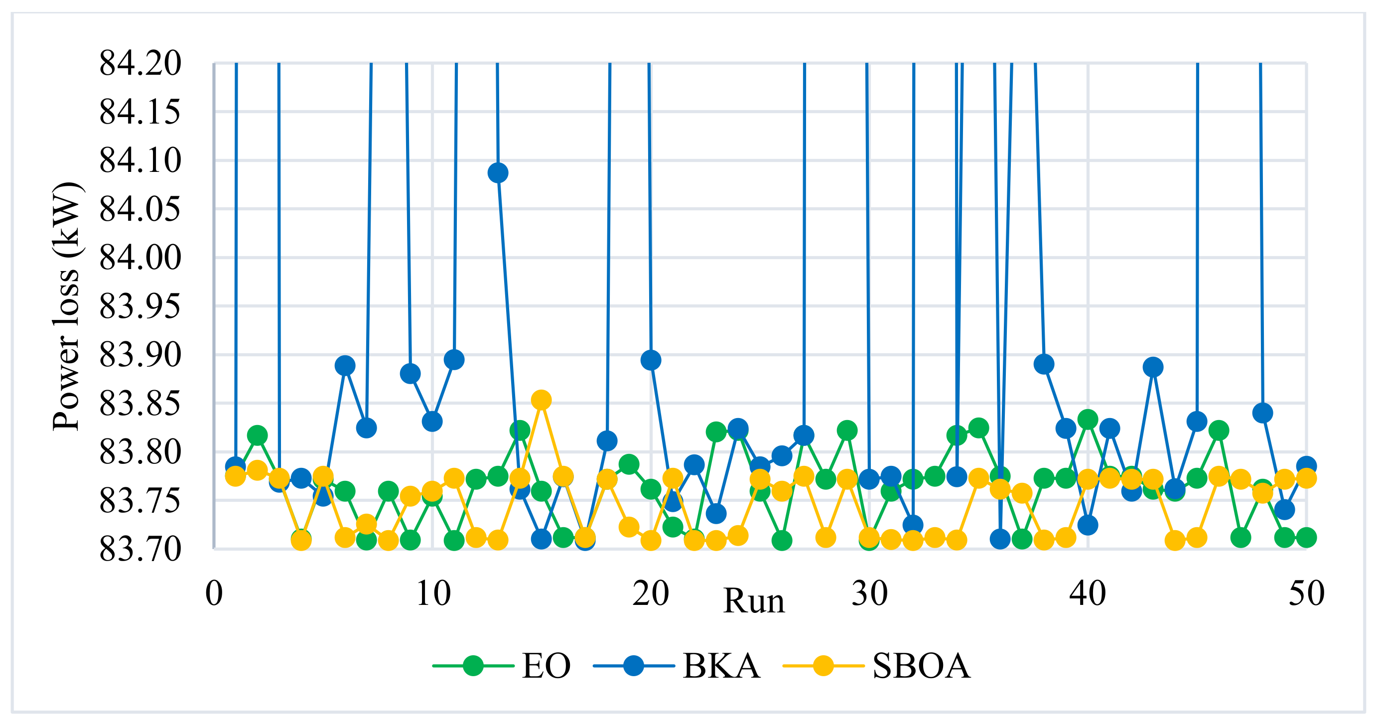
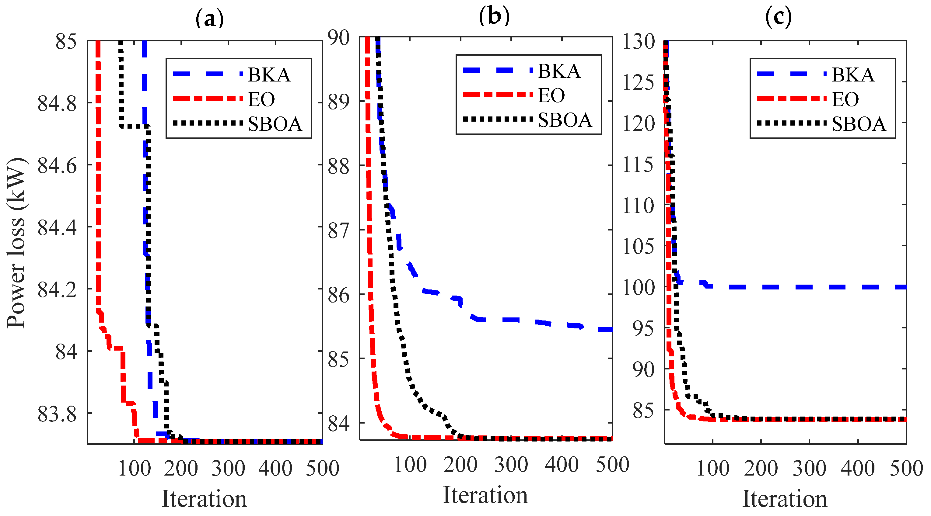
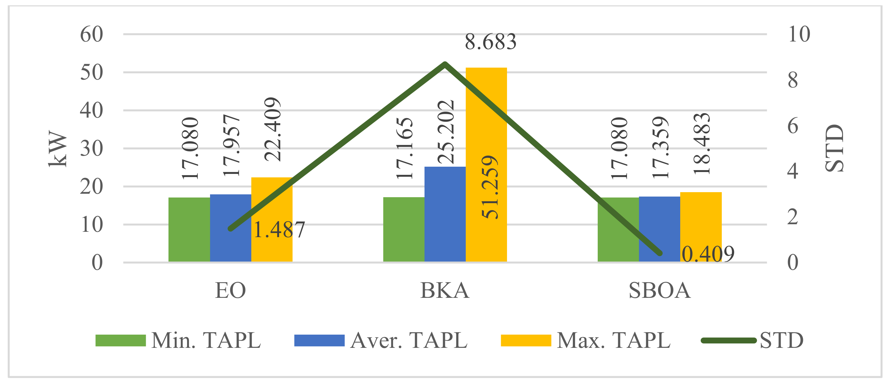
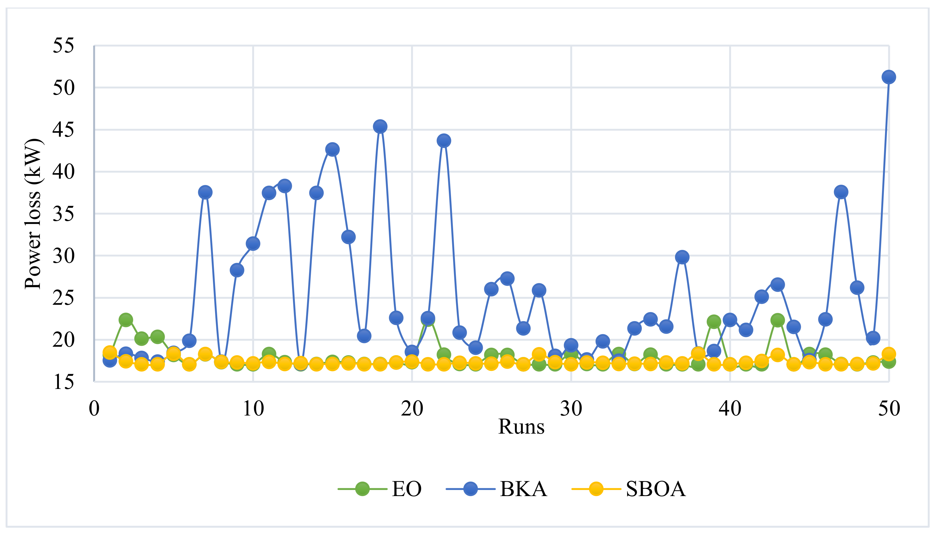
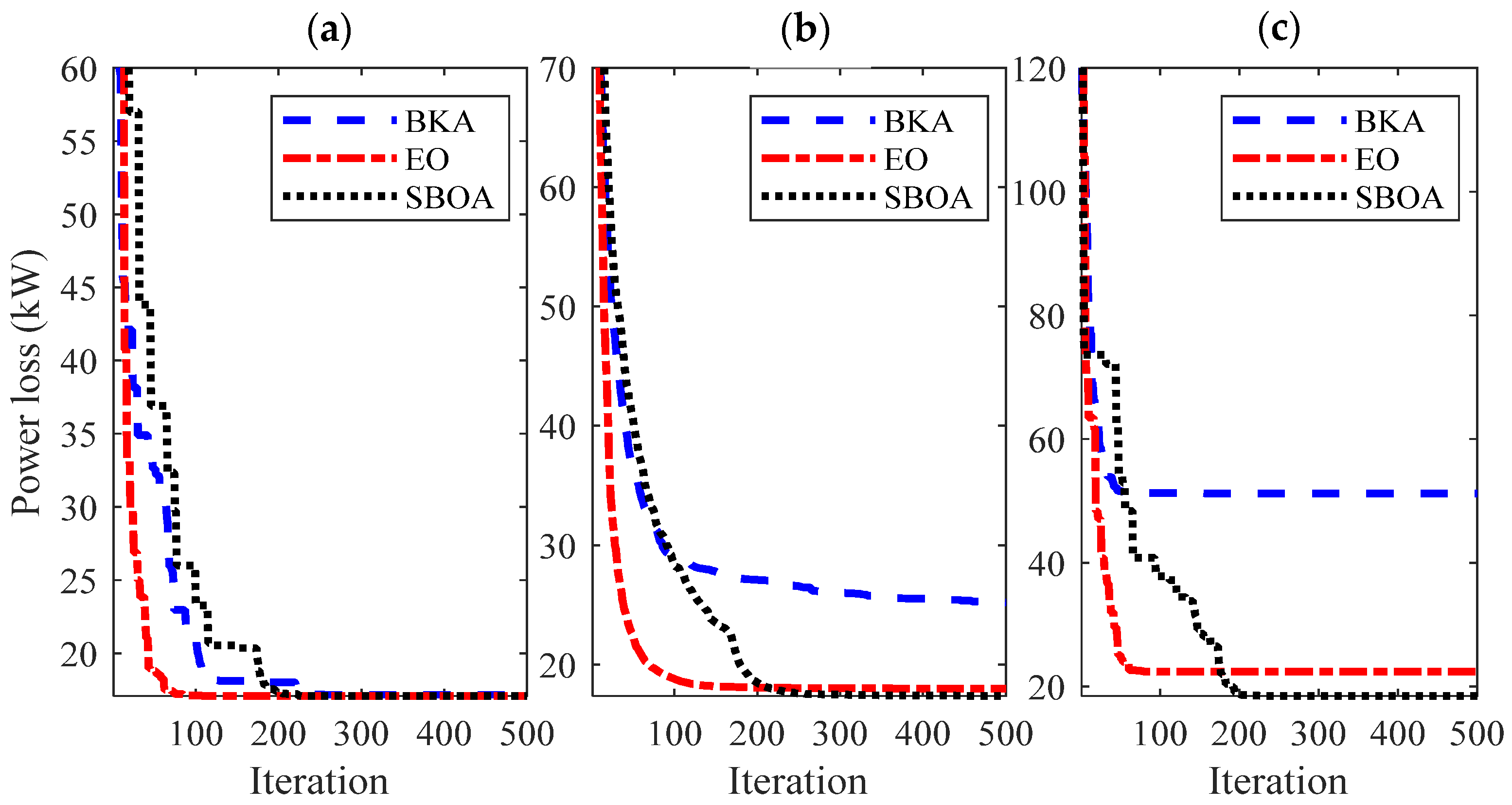
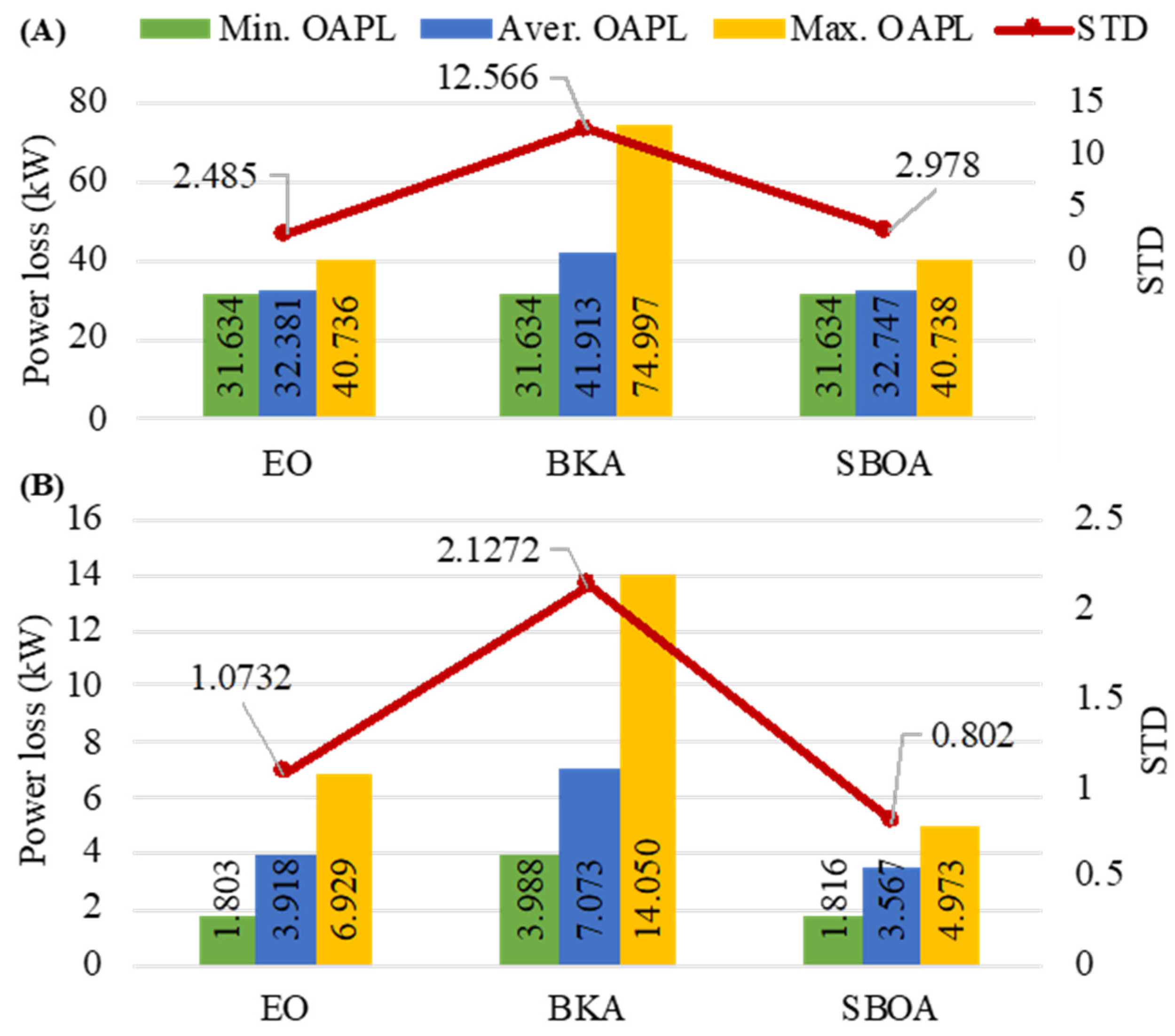
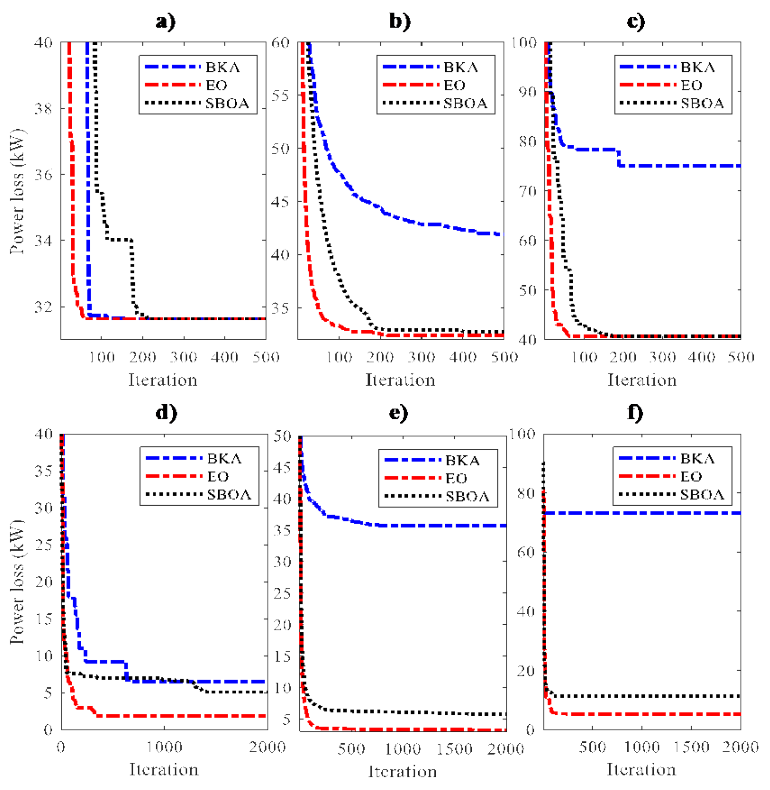
4.2. Simulation Results for Power Loss Reduction

In this section, the three applied methods are executed to optimize the placement of EVCSs and other auxiliary devices to achieve the minimum total power losses in the whole considered DPG. The result in this case is presented in the five scenarios described in the next subsection below.

Table 4. Summary of results obtained by three algorithms for Scenario 1.

Method	EO	BKA	SBOA
Best loss (kW)	225.031	225.031	225.031
Mean loss (kW)	225.031	225.031	225.031
Maximum loss (kW)	225.032	225.032	225.032
STD	4.27 × 10−5	4.31 × 10−5	4.31 × 10−5
Time execution (s)	102.532439	71.980158	1026.675761

reports that the three methods can reach the smallest loss of 255.031 kW and a very small standard deviation of about 4.10–5. The mean loss and maximum loss have the same values as the best loss. The three algorithms have the same solution for placing the three EVCS at nodes 28, 3, and 2 for Level 1, Level 2, and Level 3 stations.

Figure 3, Figure 4 and Figure 5 report the results for Scenario 2. In Figure 3, the three algorithms can reach the same best loss of 83.709 kW. The EO and SBOA reach a very small standard deviation of about 0.035, but that is about 4.4 for the BKA. Figure 4 shows that the SBOA has the most high-quality solutions, and the BKA has the most low-quality solutions. The convergence characteristics in Figure 5 indicate that the SBOA and EO can reach the same fast convergence and stable search ability, while the BKA is the worst for the manners. In summary, the three algorithms can reach the best solution with the same minimum loss, and the SBOA and EO are more stable than the BKA.

Figure 6, Figure 7 and Figure 8 report the results for Scenario 3. In Figure 6, the EO and SBOA reach the same minimum loss of 17.080 kW, whereas the BKA suffers a worse minimum loss of 17.165 kW. In addition, the mean and maximum losses of the SBOA are smaller than those of the EO and BKA. This manner can be clarified as shown in Figure 7, since more yellow points than green and blue points are located at the bottom. The convergence characteristics in Figure 8 indicate that the SBOA and EO can reach the same fast convergence for the best run; however, the EO and BKA are slower than the SBOA for the mean and worst runs. In summary, the EO and SBOA can reach the best solution, but the SBOA is the most stable algorithm for Scenario 3 of power loss reduction.

Figure 9 and Figure 10 show the results for Scenario 4 and Scenario 5. For Scenario 4, the three algorithms had the same minimum and maximum power losses; meanwhile, the EO had a smaller mean and standard deviation power loss than the SBOA and BKA. On the contrary, the EO reached the best minimum power loss for Scenario 5; however, the SBOA reached a smaller mean, maximum, and standard deviation power loss than the EO and BKA. In Figure 10, the EO is the most stable algorithm for Scenario 4, while the SBOA is the most stable for Scenario 5.

Table 5. The comparison of power loss values of the five scenarios compared to the base.

Scenario	Power Loss (kW)	Percentage of Power Loss Reduction (%)
Base	255.0185 (#)	-
1	225.031	-
2	83.709	62.80
3	17.080	92.41
4	31.634	85.94
5	1.803	99.20

The sign (#) means that the power loss value is determined based on using the forward–backward sweep technique [43] only.

below provides a detailed comparison of the EVCS’s effect in five scenarios compared to the base scenario without EVCSs and other auxiliary devices. Note that the comparison to the base scenario is performed using the optimal results obtained by the EO, the most effective method among the three applied methods.

The quantitative results presented in Table 5 clearly indicate that the power loss value of the whole network is slightly increased in the first scenario with only EVCSs placed on the grid. After that, the power loss decreased by 62.80% in Scenario 2, in which EVCSs simultaneously optimized their placements with PVU. Next, the percentage of power loss reduction in Scenario 3 was 92.41% and slightly increased to 85.94% in scenario 4, but this reduction percentage was still noticeable compared to the base scenario. Lastly, Scenario 5 witnesses a huge reduction in power loss, which was 99.20%. The conclusion is that the optimization of all types of auxiliary devices has played a crucial role in reducing the power loss increase caused by EVCSs, which can be viewed in Scenario 1.

4.3. Simulation Results for Grid Power and TVD Reduction

Table 6. Summary of results obtained by algorithms for grid power reduction.

Scenario	Grid Power (kW)	EO	BKA	SBOA	The Best Algorithm
1	Minimum	5416.521 *	5416.521 *	5416.521 *	EO, BKA, SBOA
	Mean	5416.521	5416.521	5416.521
	Maximum	5416.522	5416.522	5416.522
	STD	4.32 × 10−5 *	4.39 × 10−5 *	4.31 × 10−5 *
2	Minimum	3475.199 *	3475.215	3475.199 *	EO, SBOA
	Mean	3475.248	3484.043	3475.252
	Maximum	3475.312	3522.981	3475.334
	STD	0.036 **	11.476	0.040
3	Minimum	3408.569 *	3410.718	3408.569 *	EO, SBOA
	Mean	3410.571	3428.051	3409.602
	Maximum	3430.959	3475.832	3420.839
	STD	4.432	15.205	2.369 **
4	Minimum	3723.1242 *	3723.12521	3723.1242 *	EO, SBOA
	Mean	3725.136	3737.0985	3724.966
	Maximum	3732.2242	3763.0824	3732.637
	STD	3.7844	13.8621	3.679 *
5	Minimum	1893.2864 *	1895.97115	1893.471	EO
	Mean	1895.0782	1901.5247	1895.337
	Maximum	1896.7659	1936.1058	1899.513
	STD	1.0645 *	6.4806	1.307

and

Table 7. Summary of results obtained by algorithms for TVD reduction.

Scenario	TVD (pu)	EO	BKA	SBOA	The Best Algorithm
1	Minimum	1.838 *	1.838 *	1.838 *	EO, BKA, SBOA
	Mean	1.838	1.838	1.838
	Maximum	1.838	1.838	1.838
	STD	3.11 × 10−7 *	8.53 × 10−7	4.91 × 10−7
2	Minimum	0.6702 *	0.6702 *	0.6702 *	EO, SBOA
	Mean	0.6819	0.6924	0.6771
	Maximum	0.6926	0.7407	0.6926
	STD	0.011 **	0.0176	0.011 **
3	Minimum	0.2609 *	0.2694	0.2611	EO
	Mean	0.2821	0.3892	0.2807
	Maximum	0.5297	0.6603	0.4067
	STD	0.0457	0.0948	0.0314
4	Minimum	0.5923 *	0.5923 *	0.5923 *	EO, BKA, SBOA
	Mean	0.6113	0.6721	0.6067
	Maximum	0.6513	0.9449	0.6602
	STD	0.0276	0.0921	0.0247 **
5	Minimum	0.026 *	0.0356	0.0284	EO
	Mean	0.0368	0.0798	0.043
	Maximum	0.0499	0.2982	0.0971
	STD	0.0056 **	0.0579	0.0103

present the results from executed algorithms for the objective function of grid power and total voltage deviation reduction. In the table, we highlight the best grid power and TVD by using signal * and the most stable algorithm with the lowest standard deviation (STD) for each scenario by using signal **.

In Table 6, the three algorithms reach the same performance with the same value for minimum, mean, and maximum grid power and a very low STD of about 4.10–5 for Scenario 1. The EO and SBOA can reach the best grid power, but the EO is the most stable algorithm for Scenario 2. For Scenario 3 and Scenario 4, the EO and SBOA can reach the best grid power, but the SBOA is the most stable algorithm. For Scenario 5, the EO is the best algorithm with the best grid power and the lowest STD. The results indicate that the EO and SBOA can find the same best solutions for the same simulation scenario, so the best solutions found in the section have high reliability and validity. Since the standard deviation between the EO and SBOA is not very different, the best algorithm is selected using signal *. This means that the algorithms that can find the smallest grid power are called the best algorithms. The best algorithms are put in the last column. The EO is the best algorithm for five scenarios; meanwhile, the SBOA is the best solution for Scenarios 1–4, excluding Scenario 5. The BKA is the best solution for only Scenario 1.

In Table 7, the three algorithms reached the same value of 1.838 pu for minimum, mean, and maximum TVD and had a very low STD approximately less than 10⁻⁶ in Scenario 1. All three algorithms can reach the best grid power, but the EO and SBOA are the most stable algorithms with the smallest STD of 0.011 in Scenario 2. In Scenario 3, the EO can reach the best grid power. In Scenario 4, all three algorithms can reach the same TVD, but the SBOA is the most stable algorithm. For Scenario 5, the EO is the most effective and stable algorithm with the smallest minimum TVD and STD. In the last column, the EO is the best algorithm for five scenarios; meanwhile, the SBOA is the best solution for Scenarios 1, 2, and 4. The BKA is the best solution for only Scenarios 1 and 4.

In summary, the three applied algorithms can find the same best solutions for some of the five scenarios in two objective functions. However, the EO is the best performance algorithm for all five scenarios of two objective functions.

4.4. Discussion on Simulation Scenarios

4.4.1. The Impact of Added Active and Reactive Power Sources on Objectives

As shown in Table 6 and Table 7, the EO is more powerful than the SBOA and BKA in finding the best solutions for all scenarios. So, the section reuses the results from the EO to clarify the difference and significance of the five simulation scenarios.

Table 8. Summary of results for three single objectives obtained by EO.

Scenario	Description	Power Loss (kW)	Grid Power (kW)	TVD (pu)
Base	-	225	4026.49	1.837
1	3 EVCSs	225.031	5416.521	1.838
2	3 EVCSs + 3 PVUs	83.709	3475.199	0.6702
3	3 EVCSs + 3 PVUs + 3 CAPBs	17.08	3408.569	0.2609
4	3 EVCSs + 3 WTSs	31.6342	3723.124	0.5923
5	3 EVCSs + 3 PVUs + 3 CAPBs + 3 WTSs	1.8242	1893.2864	0.026

presents the results achieved by EO for the three objective funtions. For Scenario 1, the installation of three EVCSs with the locations nodes 28, 3, and 2 does not have a high impact on the loss and TVD. Figure 11 shows the solution of Scenario 1 with only three EVCSs. Besides, it is easy to realize that installing EVCSs close to the power source is the best solution. The EO and SBOA can reach the best grid power, but the EO is the most stable algorithm for Scenario 2. For Scenario 3 and Scenario 4, the EO and SBOA can reach the best grid power, but the SBOA is the most stable algorithm. For Scenario 5, the EO is the best algorithm with the best grid power and the lowest STD. The results indicate that the EO and SBOA can find the same best solutions for the same simulation scenario, so the best solutions found in the section have high reliability and validity. Since the standard deviation between the EO and SBOA is not very different, the best algorithm is selected using signal *. It means that the algorithms that can find the smallest grid power are called the best algorithms. The best algorithms are put in the last column. The EO is the best algorithm for five scenarios; meanwhile, the SBOA is the best solution for Scenarios 1–4, excluding Scenario 5. The BKA is the best solution for only Scenario 1.

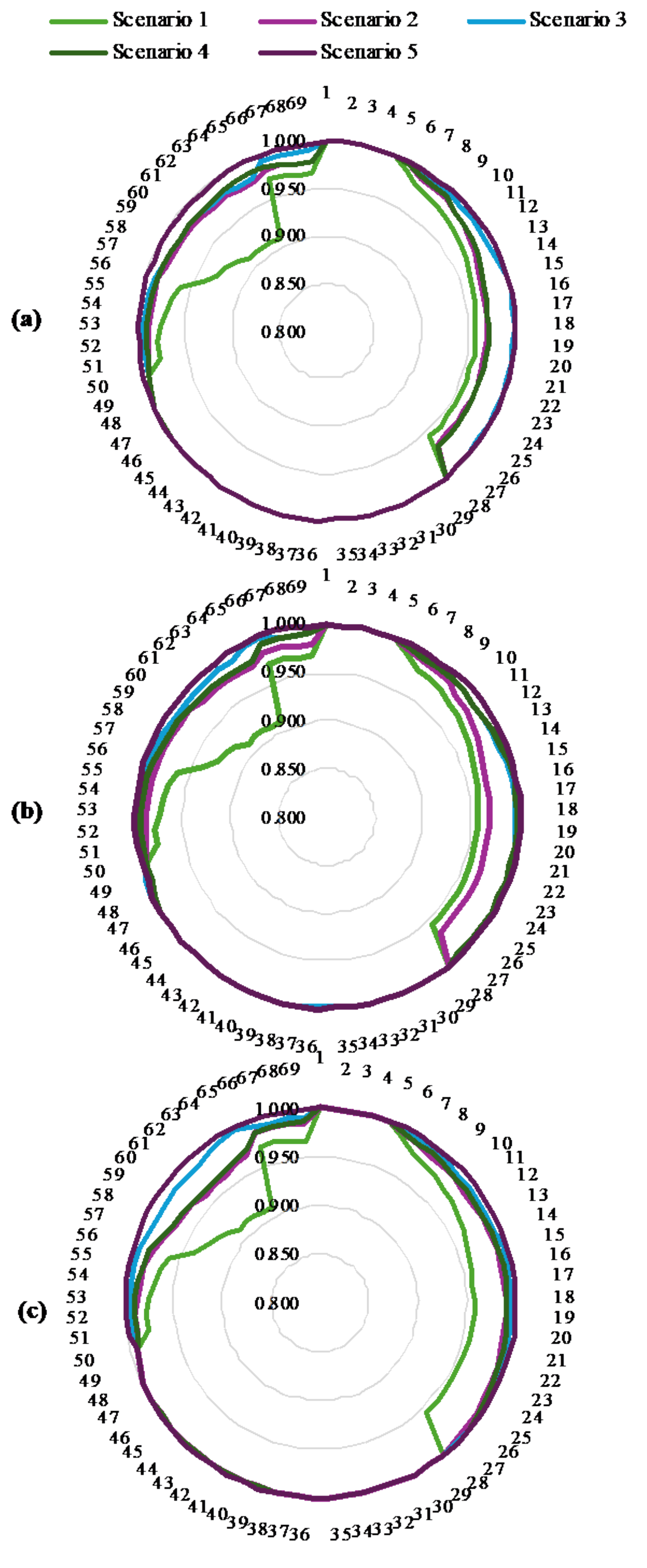
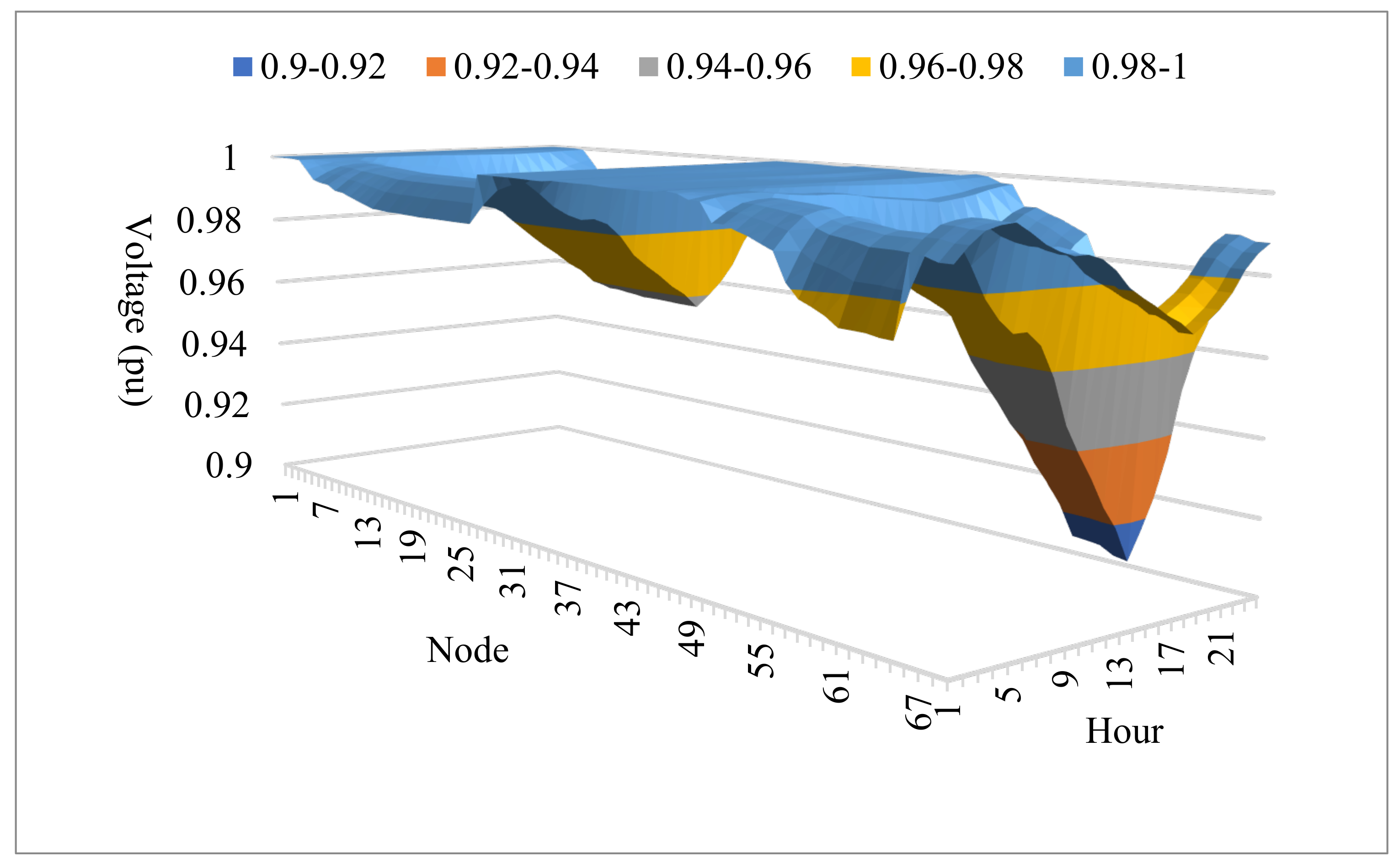
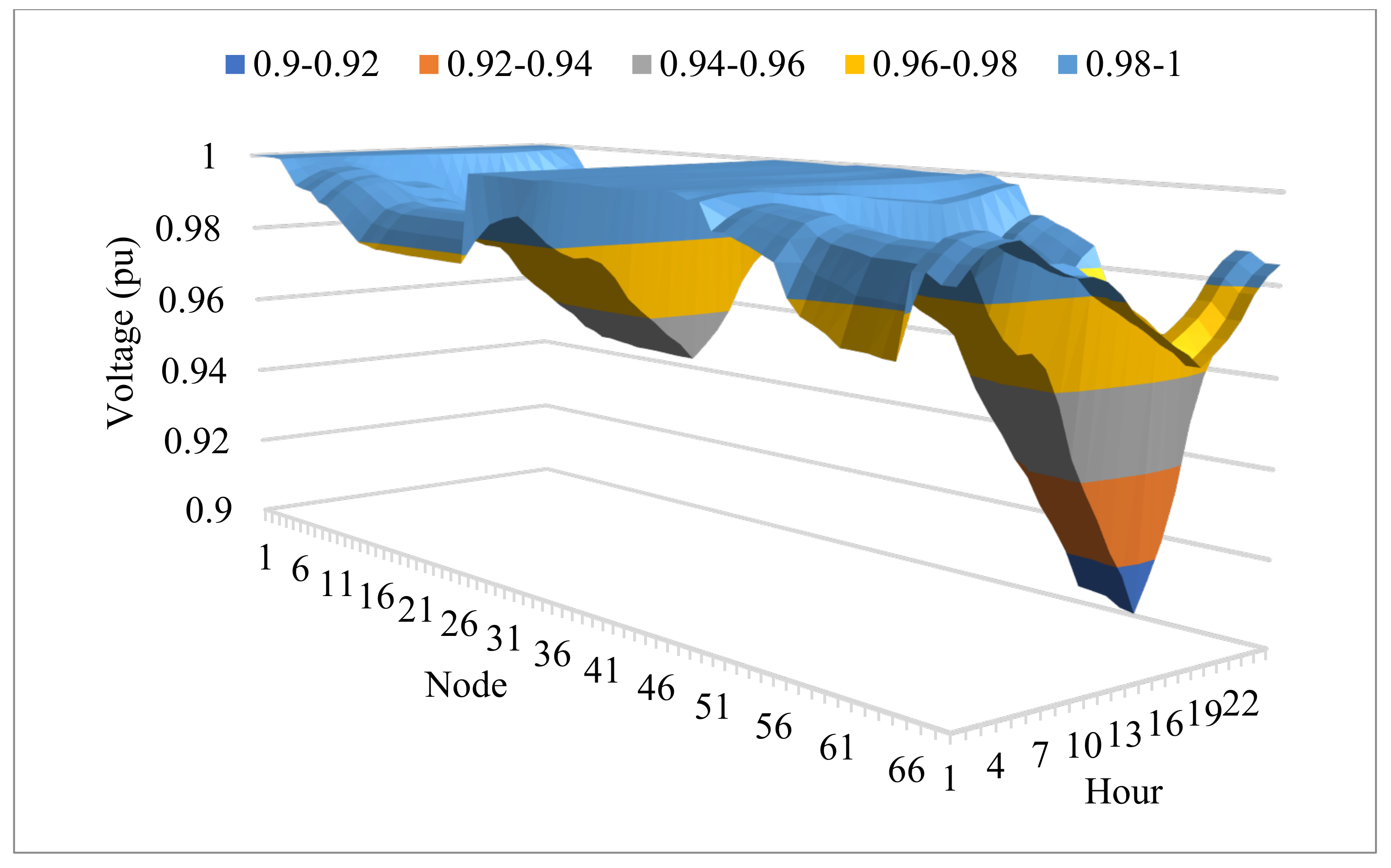
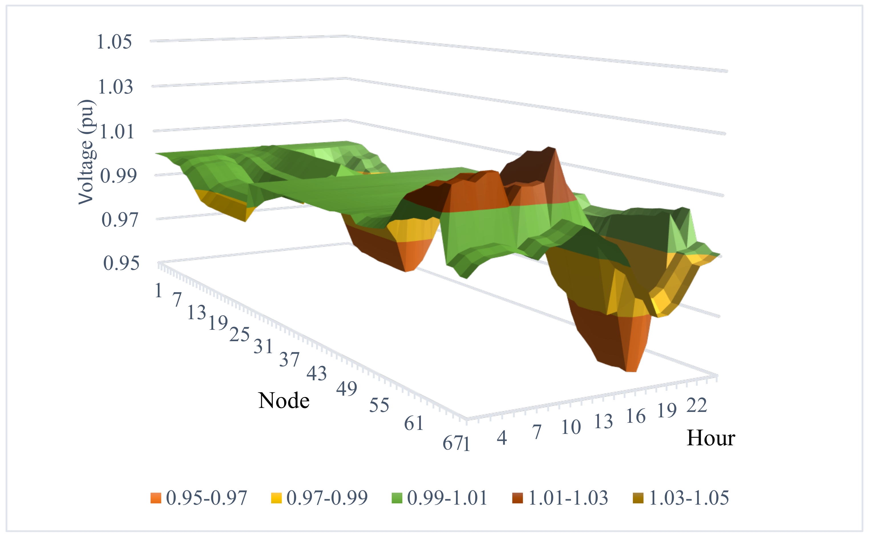
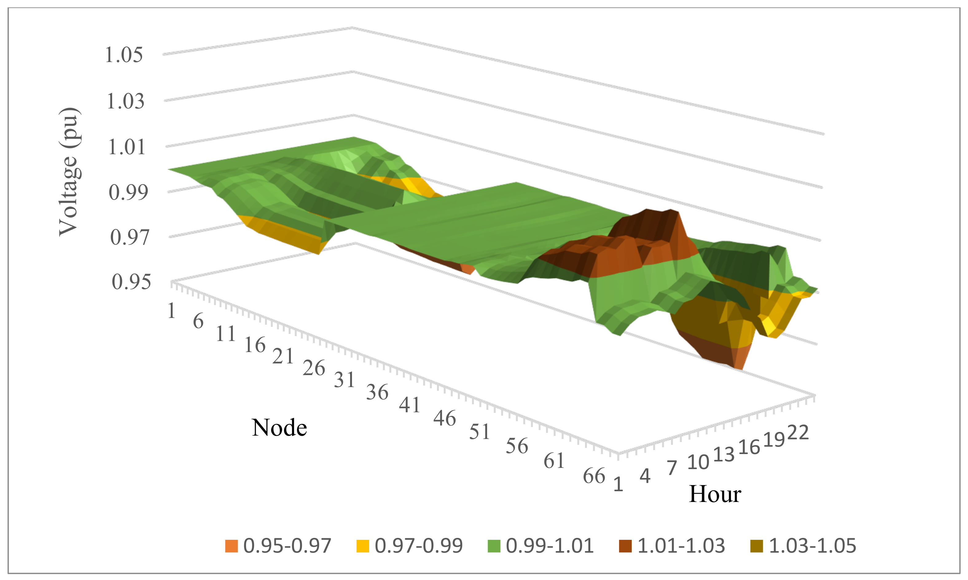
4.4.2. The Improvement of Voltage Fluctuations

In the study, the authors limited the voltage to the range between 0.9 and 1.1 pu, so all proposed solutions can satisfy the voltage constraint. The authors have plotted the voltage profile in Figure 12. There are bigger voltage differences among nodes in the network as running Scenarios 1, 2, and 4. It is clear that from nodes 50 to 69 and from nodes 6 to 27, in all three subfigures of Figure 12, the voltage of Scenario 1 is the smallest among the five scenarios. For the loss and grid power objectives, the voltage of nodes 6–27 in Scenarios 2 and 4 is a little bit greater than in Scenario 1 but much greater than in Scenarios 3 and 5. For the TVD objective in Figure 12c, Scenario 1 is also the worst, whereas the four other scenarios have a very tiny difference in comparison.

Table 9. The TVD values calculated for different objective of five scenarios.

Scenario	Loss Objective	Grid Power Objective	TVD Objective
1	1.838	1.838	1.838
2	0.916	0.916	0.67
3	0.346	0.346	0.261
4	0.816	0.816	0.592
5	0.0727	0.0578	0.0265

is established to show the voltage fluctuation. For the loss objective in the second column, the TVD is arranged in order of decrease as follows: Scenario 1, 2, 4, 3, and 5, with the values of 1.838, 0.916, 0.816, 0.346, and 0.0727. For the objectives of grid power and TVD, the orders are the same, with the values of 1.838, 0.916, 0.816, 0.346, and 0.0578 pu for grid power objective, and 1.838, 0.67, 0.261, and 0.0265 pu for TVD objective. The analysis of the total voltage deviations indicated that the fluctuations are the smallest in Scenario 5 and the second smallest in Scenario 3 for each objective function. On the other hand, the fluctuations in the same scenarios can be smallest by running the TVD objective function, excluding Scenario 1 with only the placement of EVCSs. We go back to Table 1: the active and reactive power sources that are added in Scenario 2 are three PVUs, in Scenario 3 they are three PVUs and three CAPBs, in Scenario 4 they are three WTS, and Scenario 5 placed three PVUs, three CAPBs, and three WTSs. Scenario 5, which has the highest active and reactive power sources, can reach the smallest voltage fluctuations. Both active and reactive powers are added in Scenarios 3 and 4; however, there is a difference in Scenarios 3 and 4. Scenario 3 used three PVUs and three CAPBs with different locations, but Scenario 4 employed three WTSs with the same location for generating active and reactive powers. Furthermore, each WTS can produce the reactive power from (tan(arcos(0.95)x00 = 197.21 kVar) to (tan(arcos(0.85)x600 = 371.85 kVar but each CAPB can produce 600 kVAr in maximum. So, Scenario 4 cannot reach a better voltage profile than Scenario 3.

4.4.3. The Limitations of the Study

The study focused on the technical performance of the distribution power grids in improving the loss, grid power, and TVD by optimizing the location and penetration levels of active and reactive power generation sources such as capacitors and solar- and wind-based distributed generators. In fact, simulations that were implemented focused on total voltage deviation, voltage limits, and power loss but ignored the cost of energy loss on all distribution lines [48], the total cost of investment, operation, and maintenance for wind turbines and solar photovoltaic panels [49], the total cost of building charging stations [50], and the costs of investment, operation, and maintenance for capacitor banks [51]. So, the study is unable to address economic issues. On the other hand, the study is also limited to real data and the distribution of the power grid. These shortcomings are as follows:

• Costs of electric vehicle charge stations and renewable power sources: This study only focuses on the technical factors, including total voltage deviation, voltage limits, and power loss, but neglects economic aspects, such as the cost of energy loss on all distribution lines [48], the total cost of investment, and operation and maintenance for wind turbines and solar photovoltaic panels [49], the total cost of building charging stations [50], and the costs of investment, operation, and maintenance of the capacitor banks [51]. The study did not present any economic planning strategies regarding the construction of the charge stations and renewable power, so the economic effectiveness could not be reflected by using the obtained solutions proposed by the EO and other metaheuristic algorithms. This study aimed to outline the circumstances for a distribution power grid with the installation of electric vehicle charge stations and additional sources based on wind and solar factors. Derived from the results, it concluded that the installation of charge stations led to a high electricity use demand, high power loss, and high voltage drop. However, the optimal placement of renewable energies-based distributed generators and capacitor banks could overcome faults regarding technical issues such as the overloading status of lines, high fluctuations of node voltage, and high power loss.
• The consideration of a practical distribution power network with a new building plan for an electric vehicle charge station and new installation of renewable power sources: This study employed a standard IEEE distribution power grid with 69 nodes and fixed load demand. In addition, geographical issues were not considered when selecting electric vehicle charge stations and renewable power sources. In practice, areas for constructing the stations are very large and highly expensive.
• Load demand, generation of renewable energies, and configuration of the distribution power grid: Basically, load demand and renewable power cannot be 100% accurate as predicted and obtained from the wind and solar global atlas. The change in load profiles has a high impact on the location and power of renewable power sources and capacitor banks. High load demands require high generations from renewable power sources and capacitor banks to reduce power loss and power grids and increase the voltage profile of loads. If the configuration of grids changes, the power flows will change, leading to changes in location and power supplied by renewable power sources and capacitor banks. So, the optimal placement of added electric components significantly changes under different conditions, and optimal solutions obtained by using optimization algorithms cannot be applied at each hour for a practical distribution power network. Furthermore, the inexact data influence the design problem of placing renewable power sources, i.e., selecting the location to install renewable power sources and selecting the capacity of renewable power sources. All studies cope with the same big problem, and we cannot find an absolute solution for determining the exact power of renewable energy and load demand at each hour.
• The practical implementation of EVCS placement must account for several crucial real-world factors, including traffic conditions, available space, and user convenience. Considering these factors, the research findings can become more realistic and applicable to planning and expansion processes. To further develop this research, future studies should prioritize a comprehensive investigation of the availability of potential EVCS locations. After that, a mathematical model must be formulated to restrict EVCS placement to permissible areas, ensuring optimal and feasible deployment.

4.5. Simulation for One Operating Day with Real Wind and Solar Power

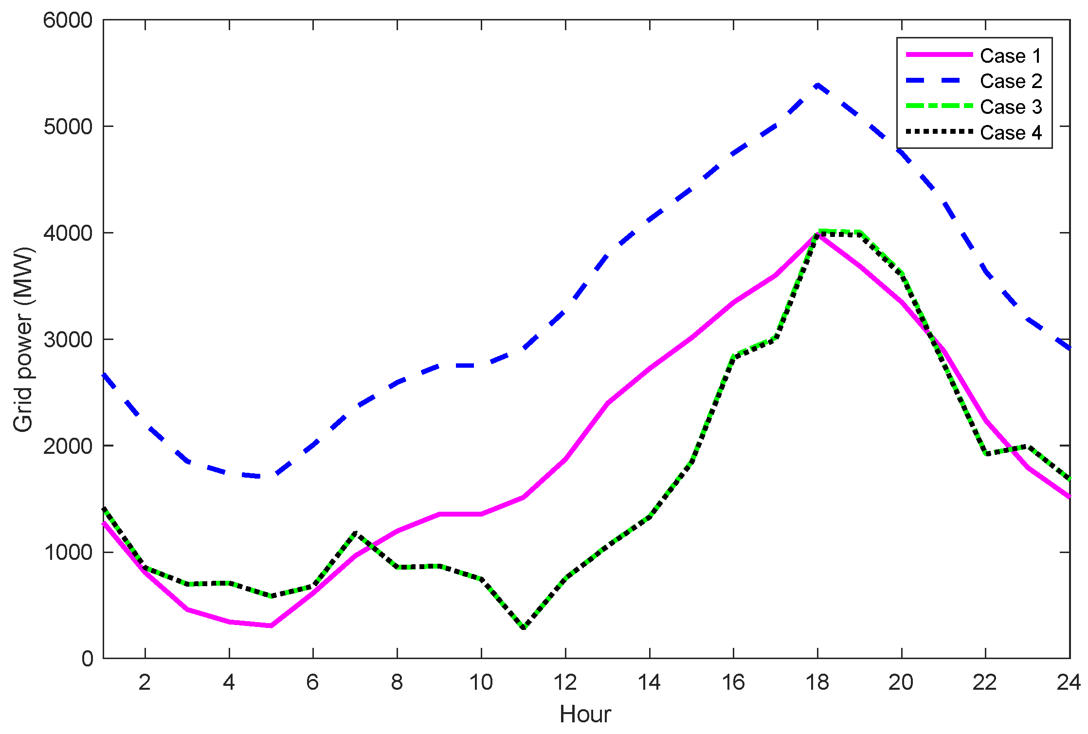
4.5.1. Study Case Simulations

In the section, the EO is selected to operate the power grid with the existing solar- and wind-distributed generators and capacitors.

• Case 1: Find grid energy for the base system without EVCS, distributed generators, and capacitors.
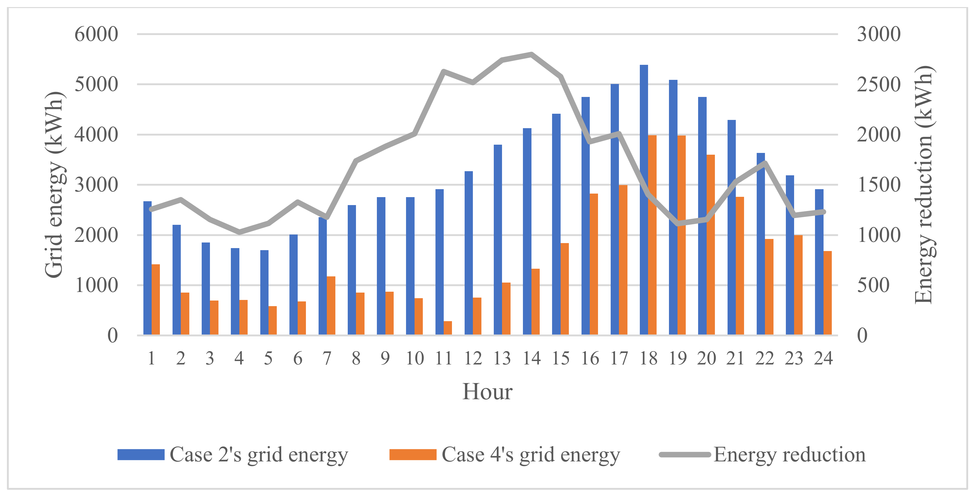
• Case 2: Find grid energy for the modified system with EVCS but without distributed generators and capacitors.
• Case 3: Find grid energy for the modified system with EVCS, solar-, and wind-based distributed generators but without capacitors.
• Case 4: Find an energy grid for the modified system with EVCSs, solar- and wind-based distributed generators, and capacitors.

As can be seen from the case descriptions above, the last two cases included wind- and solar-based distributed generators. Particularly, a 0.6 MWpeak solar-based distributed generator and a 0.5 MWpeak wind-based distributed generator are used in both Cases 3 and 4, respectively. This section concentrates on simulating grid operation over 24 h, requiring a set of generator power outputs. Solar-based distributed generators are significantly influenced by hourly solar radiation levels, as detailed in

Table 10. Radiation data within 24 h.

Hour	Radiation (W/m2)	Hour	Radiation (W/m2)	Hour	Radiation (W/m2)
1	0	9	375	17	291
2	0	10	503	18	86
3	0	11	617	19	0
4	0	12	868	20	0
5	0	13	703	21	0
6	0	14	736	22	0
7	111	15	586	23	0
8	311	16	425	25	0

from [52]. Once solar radiation data are obtained, the following formula calculates the hourly power output of the solar generator [52]:

$$P_{PVU, s, h}=\left\{\begin{array}{c}{P}_{PVU, s}^{rate}\times {\displaystyle \frac{{Ra}_h^2}{{Ra}_{std}\times R_p}}, 0<{Ra}_h<{Ra}_p\\ P_{PVU, s}^{rate}\times {\displaystyle \frac{{Ra}_h}{{Ra}_{std}}},{ Ra}_h>{Ra}_p \end{array}\right.$$

(22)

where $P_{PVU, s, h}$ (MW) is the power supplied by the PVU s at hour h with h = 1, …, 24; $P_{PVU, s}^{rate}$ (MW) is the rated power of the PVU s; ${Ra}_h$ is the solar radiation value at h hour; ${Ra}_p$(W/m²) is the value of radiation point; and ${Ra}_{std}$ is the solar radiation of the embedded environment.

To determine the hourly power output of a wind-based generator, the study relies on corresponding hourly wind speed data. These data were obtained from [53] and are presented in

Table 11. The data of wind speed within 24 h.

Hour	Wind Speed (m/s)	Hour	Wind Speed (m/s)	Hour	Wind Speed (m/s)
1	13.25	9	12.90	17	13.75
2	14	10	12.20	18	12.60
3	12.75	11	15	19	11.50
4	11.90	12	13.25	20	11.90
5	12.5	13	14.30	21	14.50
6	13.90	14	14.10	22	16.00
7	11.80	15	14.25	23	12.70
8	12.75	16	11.75	25	13.00

. While hourly wind speed values are available, the specific calculation for power output will be based on the following formula [53]:

$$P_{WT,w,h}=\left\{\begin{array}{c}0, { ws}_h<{ws}_{h,in} or {ws}_h\ge {ws}_{h,out} \\ P_{WT,w}^{rate}\times {\displaystyle \frac{{ws}_h-{ws}_{h,in}}{{ws}_{rate}^h-{ws}_{h,in}}}, {ws}_{h,in}\le {ws}_h<{ws}_{rate}^h\\ P_{WT,w}^{rate} {ws}_{rate}^h\le {ws}_h<{ws}_{h,out} \end{array}\right.$$

(23)

where $P_{WT,w,h}$ (MW) is the power output of the WTS w at hour h; $P_{WT,w}^{rate}$ (MW) is the largest amount of power output supplied by WTS w; ${ ws}_h$ (m/s) is the value of wind speed at hour h; ${ws}_{rate}^h$ (m/s) is the rated wind speed; and ${ws}_{h,in}$ and ${ws}_{h,out}$ (m/s) are the cut-in and cut-out wind speed at hour h.

Among the four cases above, Case 1 and Case 2 are simulated to find power flows without using the EO and SBOA. In contrast, the two applied algorithms are run in Case 3 and Case 4 to find the operating parameters of solar- and wind-based distributed generators and capacitors. So, Case 1 and Case 2 are simple, while Case 3 and Case 4 are more complicated. The two algorithms are run by the same population settings and maximum iteration numbers of 50 and 200, respectively. The parameters are applied to run each hour for fifty trial runs. So, the implementation comprised 50 × 24 = 1200 trial runs, and the best solution was selected for each hour. As a result, the two algorithms can reach the same minimum power grid with the same operating parameters of solar- and wind-based distributed generators and capacitors. The best results are presented and analyzed as follows:

Figure 13 presents the hourly grid power for four simulation cases, and the total grid power for one day is given in Figure 14. Case 2 needs the highest grid energy at each hour among the four cases because Case 2 supplies power to all base loads and added EVCSs. Case 1, with base load and without EVCSs, needs smaller gird energy than Case 3 and Case 4 for hours 1–7, 18–20, and 23–24. Case 3 and Case 4 supply full power to all base load and EVCSs, but the two cases are equipped with solar- and wind-based distributed generators, as well as capacitors. The deviation between Case 3 and Case 4 cannot be distinguished; however, the total grid power of one day of Case 3 and Case 4 is different, as shown in Figure 14. Case 4 reaches the smallest grid energy of 39,578.9 kWh, while Case 3 has 39,713.9 kWh. Case 4 requires a smaller energy than Case 3 by 134.5 kWh, corresponding to 0.34%. The energy reduction is the result of installing capacitors in Case 4. Compared to Case 2, Case 4 needs a smaller energy of 40,574.3 kWh, corresponding to 50.62%. The energy reduction of 50.62% is the result of installing renewable energy-based distributed generators and capacitors in Case 4 compared to Case 2.

The active power balance constraint satisfaction in Case 1 and Case 2 is clearly seen in Figure 15. The grid power is equal to the sum of load power and loss power at each hour in Figure 15A, while the grid power is equal to the sum of load power, loss power, and EVCSs’ power. Figure 16 presents the satisfaction of active power balance constraints in Case 3 and Case 4. The two cases have the same manner: the total grid power, PVUs’ power, and WTSs’ power are equal to the total loss power, load power, and EVCSs’ power.

Figure 17, Figure 18, Figure 19 and Figure 20 present the voltage profiles of the four cases. Case 1 and Case 2 have an extensive range of voltage from 0.9 to 1 pu. Here, voltage values from 0.9 to 0.95 pu violate the lower voltage limit set to 0.95 pu. Nodes 57 to 69 have low voltage from 0.9 to 0.96 pu within hours 10–20. Case 2 has approximately the same voltage profile as Case 1.

The voltage profile in Case 3 is much improved as compared to Case 1 and Case 2. The range between 0.9 and 0.95 pu does not appear in Figure 19. Case 4 shown in Figure 20 is greater than Case 3 in improving the voltage profile. The nodes with low voltages from 0.95 to 0.97 pu are fewer. In fact, the areas in blue and orange are smaller in Case 4 than in Case 3. This effectiveness of voltage improvement is due to the installation of capacitors. The results indicate that the installation of EVCSs needs higher energy from the power grid and also causes the voltage to get worse, even if the voltage violates the lower limit. The installation of renewable power sources is useful in improving the energy demand and voltage; however, the additional installation of capacitors is more powerful in reducing the energy from the grid and improving the voltage.

4.5.2. The Benefit of Systems with CAPBs, PVUs, and WTSs

The section simulates different cases corresponding to different added electric components to find the best grid power supplied by the conventional power sources at the slack node. The four cases calculated the total grid energy supplied to base loads and/or EVCSs. Here, Case 2 and Case 4 are two special cases: Case 2 with only EVCSs and Case 4 with both EVCSs and other added power sources such as CAPBs, WTSs, and PVUs. This section calculates the benefits thanks to the optimal placement and operation of these added power sources in terms of money and payback period.

When the total costs of the renewable power sources and capacitor banks are exactly determined, their placement becomes more practical and effective in the distribution of power grids. Suppose that this is a project with 20 years and all 365 days of each year have the same load demand and the same generation for renewable power sources. So, the benefit of the system can be obtained by

$${BF}_{sys}=\left[N_{year}.365.\sum _{h=1}^{24}({Price}_h. ∆E_h)\right]-{Cost}_{PV}-{Cost}_{Wind}-{Cost}_{Cap}$$

(24)

where $N_{year}$ is the number of years for the project with the renewable power sources and capacitor banks; ${Price}_h$ is the electricity price at the hth hour; $∆E_h$ is the grid energy reduction at the hth hour; ${Cost}_{PV}$ and ${Cost}_{Wind}$ are the sum of capital, operation, and maintenance costs for solar and wind power sources over 20 years; and ${Cost}_{Cap}$ is the sum of capaictal cost and annual cost over 20 years.

$∆E_h$ is obtained by calculating the difference between Case 2 and Case 4’s grid power. So, the grid energy reduciton is the benefit of Case 4 compared to Case 2. The grid energy of Case 2, Case 4, and the hourly grid energy reduction are plotted in Figure 21.

For economic issues, Case 4 must pay more costs than Case 2 for buying, operating, and maintaining PVUs, CAPBs, and WTSs. The electric price is 96 (USD/MWh) [54], and other costs regarding capacitors, PVUs, and WTSs are given in

Table 12. The price information of added power sources.

Power Source	Capital Price	Operating and Maintenance Price	Annual Price
Wind turbines [55]	1882 (USD/kW)	0.01 (USD/kWh)	-
Solar panel [56]	770 (USD/kW)	0.01 (USD/kWh)	-
Capacitor (600 kVar)	1320 (USD) [57]	-	0.22 (USD/kVar year) [58]

[55,56,57,58].

From the results reported for Case 2 and Case 4 shown in Figure 20, the total grid energy per day for Case 2 and Case 4 and the grid energy reduction are calculated and reported in

Table 13. Gird energy and grid costs for Case 2 and Case 4.

Parameters	Total Grid Energy (kWh/day)	Grid Cost (USD/day)	Grid Cost (USD/20 Years)
Case 2	80,153.1037	7694.69795	56,171,295.1
Case 4	39,578.8509	3799.56969	27,736,858.7
Cost Reduction (USD)			28,434,436.3

. Case 2 used a total grid energy of 80,153.1037 kWh/day, while Case 4 used a small total energy of 39,578.8509 kWh/day. The grid costs per day and for 20 years were obtained by using the formulas (electric price $\times$ total grid energy) and (electric price $\times$ total grid energy $\times$ 365 days $\times$ 20 years), respectively. As a result, Case 4 can save a cost of USD 28,434,436.3 for a period of 20 years.

To calculate the payback period, we calculate the capital cost and operation and maintenance (O & M) cost for PVUs and WTSs, and the capital cost and annual cost for CAPBs. The summary of costs is given in Table 13. The calculation of costs is obtained by using the following formulas:

-

Capital cost (USD) = Capital price $\times$ rated power

-

Annual cost (USD/20 years) = Annual price $\times$ rated power $\times$ 20 years

-

O & M cost (USD/20 years) = O & M price $\times$

-

Total generation $\times$ 365 days $\times$ 20 years

-

Total cost for PVUs and WTs = Capital cost + O & M cost (USD/20 years)

-

Total cost for CAPBs = Capital cost + Annual cost

As shown in

Table 14. Costs of added power sources for Case 4.

Device-Rated Power	Total Gen. (kWh/day)	Capital Cost (USD)	Annual Cost (20 Years)	O & M Cost (USD/20 Years)	Total Cost (USD)
PVU1-500 kW	3217.98	385,000	-	234,912.54	619,912.5447
PVU2-500 kW	3216.89	385,000	-	234,832.71	619,832.705
PVU3-500 kW	3217.38	385,000	-	234,868.43	619,868.4299
WTS1-600 kW	9825.21	1,129,200	-	717,240.00	1,846,439.998
WTS2-600 kW	9825.72	1,129,200	-	717,277.38	1,846,477.383
WTS3-600 kW	9824.12	1,129,200	-	717,160.94	1,846,360.941
CAPB1-600 kVar	-	1320	2640	-	3960
CAPB2-600 kVar	-	1320	2640	-	3960
CAPB3-600 kVar	-	1320	2640	-	3960
Total costs for all devices					7,410,772

, the total costs for added electric components are USD 7,410,772. So, the benefit can be obtained by using the cost reduction-the total costs of all devices, equaling (28,434,436.3–7,410,772) = USD 21,023,664.3. The benefit is equal to 21,023,664.3/7,410,772 = 2.84 times the total costs. The benefit per year is obtained, and then the payback period is determined as follows:

-

Benefit per year = total cost reduction/20 = 1,421,721.82 (USD/year)

-

Payback period = total costs/benefit per year = 5.21 (years)

So, we can obtain the total costs of added devices, including the capital cost, O & M cost, and annual cost, after 5 years and 2.4 months.

5. Conclusions

The study optimized power loss, grid power, and total voltage deviation for the IEEE 69-node distribution power grid by running three algorithms, including the black kite algorithm (BKA), equilibrium optimizer (EO), and secretary bird optimization algorithm (SBOA). The three algorithms were run to optimize the location of added electric vehicle charge stations, wind- and solar-based distributed generators, and capacitor banks to reach the single objectives in one single period. The results from the three algorithms, including the power loss, grid power, and total voltage deviation, are compared to each other to find the most suitable algorithm. The SBOA was more stable than the EO for simple cases with only the charge station placement, both charge stations, and PVUs. In other cases where the charge stations, capacitors, PVUs, and WTSs were placed, the EO was more powerful than the SBOA. So, the last case, which had one operating day, was only applied for the EO to optimize the grid energy and voltage profile. The EO was run for two cases: Case 3 with PVUs and WTSs and Case 4 with PVUs, WTSs, and capacitors. In addition, Case 1 with all the base loads and Case 2 with all the base loads and charge stations were also run to find the grid energy. The results can be summarized as follows:

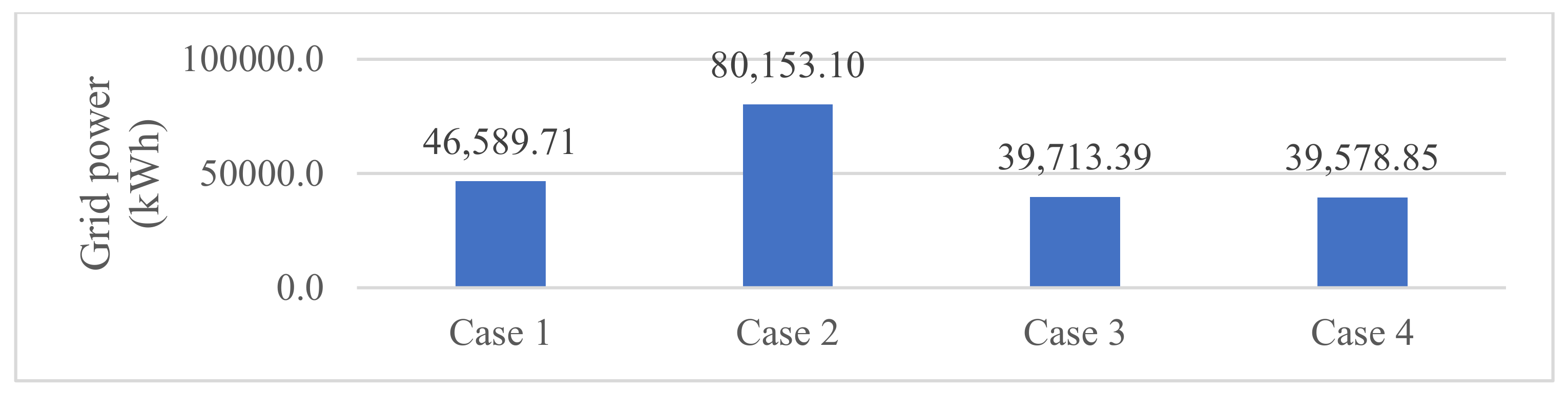
• Case 2 provided the highest energy of 80,153.1 kWh, while Case 3 and Case 4 provided the energy of 39,713.4 kWh and 39,578.9 kWh. So, Case 4 can reduce the energy by greater than 50% of Case 2 and 0.34% of Case 3.
• Case 1 and Case 2 suffered the lowest voltage in the range between 0.9 and 0.95 Pu, violating the lower voltage limit of 0.5 Pu. Case 4 reached the best voltage profile among the four cases, with all nodes in the range from 0.95 to 1.0 Pu. The nodes with 0.95 and 0.97 Pu were the fewest in Case 4, and the remaining nodes were in the range of 0.97 and 1.0 Pu.

The results above show the significant contributions of the study in reducing the energy demand from the power grids, which were supplied by conventional power plants. In addition, the voltage profile was much improved within the allowable range. However, the study must overcome several limitations that could be more practical in the distribution of power grids. Basically, charge stations use electric power devices to produce harmonics that harm power quality. The bad power quality can negatively impact base loads in distribution systems. In addition, the voltage fluctuations or instability issues that happen when faults or disturbances on the grid occur are also a big challenge in the distribution of power grids with EVCSs and renewable power sources. So, future work needs to consider the harmonic generation of the devices and solutions to eliminate the harmonics and faults causing voltage fluctuation and other instability issues. On the other hand, the availability of placing EVCSs at the actual location on the ground must be thoroughly evaluated. Moreover, real distribution power grids, real generation of renewable sources, policies for installing charge stations, and total costs of EVCSs and other electric components will be considered in future work. The next studies can present a real distribution power grid phenomenon in improving electric vehicles charge stations.

References

1. Mariappan, S.; David Raj, A.; Kumar, S.; Chatterjee, U. Global Warming Impacts on the Environment in the Last Century. In Springer Climate; Springer Science and Business Media B.V.: Cham, Switzerland, 2022; pp. 63–93. [Google Scholar]
2. Rawat, A.; Kumar, D.; Khati, B.S. A Review on Climate Change Impacts, Models, and Its Consequences on Different Sectors: A Systematic Approach. J. Water Clim. Chang. 2024, 15, 104–126. [Google Scholar] [CrossRef]
3. Yoro, K.O.; Daramola, M.O. CO2 Emission Sources, Greenhouse Gases, and the Global Warming Effect. In Advances in Carbon Capture; Elsevier: Amsterdam, The Netherlands, 2020; pp. 3–28. [Google Scholar]
4. Paris Agreement Climate Change. Available online: https://unfccc.int/process-and-meetings/the-paris-agreement (accessed on 2 January 2025).
5. Riesz, J.; Sotiriadis, C.; Ambach, D.; Donovan, S. Quantifying the Costs of a Rapid Transition to Electric Vehicles. Appl. Energy 2016, 180, 287–300. [Google Scholar] [CrossRef]
6. Chen, Y.; Chen, Y.; Lu, Y. Spatial Accessibility of Public Electric Vehicle Charging Services in China. ISPRS Int. J. Geoinf. 2023, 12, 478. [Google Scholar] [CrossRef]
7. Kaya, Ö.; Alemdar, K.D.; Campisi, T.; Tortum, A.; Çodur, M.K. The Development of Decarbonisation Strategies: A Three-Step Methodology for the Suitable Analysis of Current Evcs Locations Applied to Istanbul, Turkey. Energies 2021, 14, 2756. [Google Scholar] [CrossRef]
8. Haces-Fernandez, F. Risk Assessment Framework for Electric Vehicle Charging Station Development in the United States as an Ancillary Service. Energies 2023, 16, 8035. [Google Scholar] [CrossRef]
9. Sheng, K.; Dibaj, M.; Akrami, M. Analysing the Cost-Effectiveness of Charging Stations for Electric Vehicles in the U.K.’s Rural Areas. World Electr. Veh. J. 2021, 12, 232. [Google Scholar] [CrossRef]
10. Rathnayake, R.M.D.I.M.; Jayawickrama, T.S.; Melagoda, D.G. The Feasibility of Establishing Electric Vehicle Charging Stations at Public Hotspots in Sri Lanka. In Proceedings of the MERCon 2019—Proceedings, 5th International Multidisciplinary Moratuwa Engineering Research Conference, Moratuwa, Sri Lanka, 3–5 July 2019; Institute of Electrical and Electronics Engineers Inc.: Piscataway, NJ, USA, 2019; pp. 510–514. [Google Scholar]
11. Liu, G.; Kang, L.; Luan, Z.; Qiu, J.; Zheng, F. Charging Station and Power Network Planning for Integrated Electric Vehicles (EVs). Energies 2019, 12, 2595. [Google Scholar] [CrossRef]
12. Zhang, Y.; Zhang, Q.; Farnoosh, A.; Chen, S.; Li, Y. GIS-Based Multi-Objective Particle Swarm Optimization of Charging Stations for Electric Vehicles. Energy 2019, 169, 844–853. [Google Scholar] [CrossRef]
13. Bilal, M.; Rizwan, M. Integration of Electric Vehicle Charging Stations and Capacitors in Distribution Systems with Vehicle-to-Grid Facility. Energy Sources Part A Recovery Util. Environ. Eff. 2021. [Google Scholar] [CrossRef]
14. Liu, Z.; Wen, F.; Ledwich, G. Optimal Planning of Electric-Vehicle Charging Stations in Distribution Systems. IEEE Trans. Power Deliv. 2013, 28, 102–110. [Google Scholar] [CrossRef]
15. Zeb, M.Z.; Imran, K.; Khattak, A.; Janjua, A.K.; Pal, A.; Nadeem, M.; Zhang, J.; Khan, S. Optimal Placement of Electric Vehicle Charging Stations in the Active Distribution Network. IEEE Access 2020, 8, 68124–68134. [Google Scholar] [CrossRef]
16. Ahmad, F.; Khalid, M.; Panigrahi, B.K. An Enhanced Approach to Optimally Place the Solar Powered Electric Vehicle Charging Station in Distribution Network. J. Energy Storage 2021, 42, 103090. [Google Scholar] [CrossRef]
17. Chen, L.; Xu, C.; Song, H.; Jermsittiparsert, K. Optimal Sizing and Sitting of EVCS in the Distribution System Using Metaheuristics: A Case Study. Energy Rep. 2021, 7, 208–217. [Google Scholar] [CrossRef]
18. Mehrjerdi, H.; Hemmati, R. Stochastic Model for Electric Vehicle Charging Station Integrated with Wind Energy. Sustain. Energy Technol. Assess. 2020, 37, 100577. [Google Scholar] [CrossRef]
19. Hafez, O.; Bhattacharya, K. Optimal Design of Electric Vehicle Charging Stations Considering Various Energy Resources. Renew Energy 2017, 107, 576–589. [Google Scholar] [CrossRef]
20. Dai, Q.; Liu, J.; Wei, Q. Optimal Photovoltaic/Battery Energy Storage/Electric Vehicle Charging Station Design Based on Multi-Agent Particle Swarm Optimization Algorithm. Sustainability 2019, 11, 1973. [Google Scholar] [CrossRef]
21. Zhang, M.; Yan, Q.; Guan, Y.; Ni, D.; Agundis Tinajero, G.D. Joint Planning of Residential Electric Vehicle Charging Station Integrated with Photovoltaic and Energy Storage Considering Demand Response and Uncertainties. Energy 2024, 298, 131370. [Google Scholar] [CrossRef]
22. Chowdhury, R.; Mukherjee, B.K.; Mishra, P.; Mathur, H.D. Performance Assessment of a Distribution System by Simultaneous Optimal Positioning of Electric Vehicle Charging Stations and Distributed Generators. Electr. Power Syst. Res. 2023, 214, 108934. [Google Scholar] [CrossRef]
23. Ahmad, F.; Iqbal, A.; Ashraf, I.; Marzband, M.; Khan, I. Optimal Location of Electric Vehicle Charging Station and Its Impact on Distribution Network: A Review. Energy Rep. 2022, 8, 2314–2333. [Google Scholar] [CrossRef]
24. Yuvaraj, T.; Devabalaji, K.R.; Thanikanti, S.B.; Aljafari, B.; Nwulu, N. Minimizing the Electric Vehicle Charging Stations Impact in the Distribution Networks by Simultaneous Allocation of DG and DSTATCOM with Considering Uncertainty in Load. Energy Rep. 2023, 10, 1796–1817. [Google Scholar] [CrossRef]
25. Kathiravan, K.; Rajnarayanan, P.N. Application of AOA Algorithm for Optimal Placement of Electric Vehicle Charging Station to Minimize Line Losses. Electr. Power Syst. Res. 2023, 214, 108868. [Google Scholar] [CrossRef]
26. Krishnamurthy, N.K.; Sabhahit, J.N.; Jadoun, V.K.; Gaonkar, D.N.; Shrivastava, A.; Rao, V.S.; Kudva, G. Optimal Placement and Sizing of Electric Vehicle Charging Infrastructure in a Grid-Tied DC Microgrid Using Modified TLBO Method. Energies 2023, 16, 1781. [Google Scholar] [CrossRef]
27. Karmaker, A.K.; Hossain, M.A.; Pota, H.R.; Onen, A.; Jung, J. Energy Management System for Hybrid Renewable Energy-Based Electric Vehicle Charging Station. IEEE Access 2023, 11, 27793–27805. [Google Scholar] [CrossRef]
28. Yuvaraj, T.; Devabalaji, K.R.; Thanikanti, S.B.; Pamshetti, V.B.; Nwulu, N.I. Integration of Electric Vehicle Charging Stations and DSTATCOM in Practical Indian Distribution Systems Using Bald Eagle Search Algorithm. IEEE Access 2023, 11, 55149–55168. [Google Scholar] [CrossRef]
29. Alshareef, S.; Fathy, A. Efficient Red Kite Optimization Algorithm for Integrating the Renewable Sources and Electric Vehicle Fast Charging Stations in Radial Distribution Networks. Mathematics 2023, 11, 3305. [Google Scholar] [CrossRef]
30. Khalid, M.R.; Khan, I.A.; Hameed, S.; Asghar, M.S.J.; Ro, J. A Comprehensive Review on Structural Topologies, Power Levels, Energy Storage Systems, and Standards for Electric Vehicle Charging Stations and Their Impacts on Grid. IEEE Access 2021, 9, 128069–128094. [Google Scholar] [CrossRef]
31. Parajuli, A.; Gurung, S.; Chapagain, K. Optimal Placement and Sizing of Battery Energy Storage Systems for Improvement of System Frequency Stability. Electricity 2024, 5, 662–683. [Google Scholar] [CrossRef]
32. Saldanha, J.J.; Nied, A.; Trentini, R.; Kutzner, R. AI-based optimal allocation of BESS, EV charging station and DG in distribution network for losses reduction and peak load shaving. Electr. Power Syst. Res. 2024, 234, 110554. [Google Scholar] [CrossRef]
33. Alizadeh, M.; Meegahapola, L.; Amani, A.M.; Jalili, M.; Seilsepour, A. Optimal Planning Framework for Battery Energy Storage Systems and Electric Vehicle Charging Stations in Distribution Networks. In Proceedings of the 2024 IEEE International Conference on Industrial Technology (ICIT), Bristol, UK, 25–27 March 2024; pp. 1–6. [Google Scholar] [CrossRef]
34. Zhang, W.; Yang, X.; Huang, Q.; Yan, S.; Xia, J.; Zhao, Y. EVCS Joint BESS Optimal Planning Based on MOTEO Algorithm. In Proceedings of the 2024 IEEE 2nd International Conference on Power Science and Technology (ICPST), Dali, China, 9–11 May 2024; pp. 1949–1954. [Google Scholar] [CrossRef]
35. Kazemtarghi, A.; Mallik, A. A two-stage stochastic programming approach for electric energy procurement of EV charging station integrated with BESS and PV. Electr. Power Syst. Res. 2024, 232, 110411. [Google Scholar] [CrossRef]
36. Eid, A.; Abdel-Salam, M. Management of electric vehicle charging stations in low-voltage distribution networks integrated with wind turbine–battery energy storage systems using metaheuristic optimization. Eng. Optim. 2024, 56, 1335–1360. [Google Scholar] [CrossRef]
37. Kumar, P.M.; Dhilipkumar, R.; Geethamahalakshmi, G.; Sujatha, M. Efficient distribution network based on photovoltaic fed electric vehicle charging station using WSO-RBFNN approach. J. Energy Storage 2025, 106, 114728. [Google Scholar] [CrossRef]
38. Wang, J.; Wang, W.; Hu, X.; Qiu, L.; Zang, H. Black-Winged Kite Algorithm: A Nature-Inspired Meta-Heuristic for Solving Benchmark Functions and Engineering Problems. Artif. Intell. Rev. 2024, 57, 98. [Google Scholar] [CrossRef]
39. Faramarzi, A.; Heidarinejad, M.; Stephens, B.; Mirjalili, S. Equilibrium Optimizer: A Novel Optimization Algorithm. Knowl Based Syst. 2020, 191, 105190. [Google Scholar] [CrossRef]
40. Fu, Y.; Liu, D.; Chen, J.; He, L. Secretary Bird Optimization Algorithm: A New Metaheuristic for Solving Global Optimization Problems. Artif. Intell. Rev. 2024, 57, 123. [Google Scholar] [CrossRef]
41. Vijay, V.; Venkaiah, C.; Mallesham, V.K.D. Meta Heuristic Algorithm Based Multi Objective Optimal Planning of Rapid Charging Stations and Distribution Generators in a Distribution System Coupled with Transportation Network. Adv. Electr. Electron. Eng. 2023, 20, 493–504. [Google Scholar] [CrossRef]
42. Guerraiche, K.; Midouni, F.; Sahraoui, N.E.; Dekhici, L. Application of Equilibrium Optimizer Algorithm for Solving Linear and Non Linear Coordination of Directional Overcurrent Relays. Adv. Electr. Electron. Eng. 2023, 20, 537–548. [Google Scholar] [CrossRef]
43. Teng, J.H.; Chang, C.Y. Backward/forward sweep-based harmonic analysis method for distribution systems. IEEE Trans. Power Deliv. 2007, 22, 1665–1672. [Google Scholar] [CrossRef]
44. Duong, M.Q.; Pham, T.D.; Nguyen, T.T.; Doan, A.T.; Tran, H.V. Determination of optimal location and sizing of solar photovoltaic distribution generation units in radial distribution systems. Energies 2019, 12, 174. [Google Scholar] [CrossRef]
45. Poudyal, R.; Loskot, P.; Parajuli, R. Techno-Economic Feasibility Analysis of a 3-KW PV System Installation in Nepal. Renew. Wind Water Sol. 2021, 8, 5. [Google Scholar] [CrossRef]
46. Hadzhiev, I.; Malamov, D.; Balabozov, I.; Yatchev, I. Study of Operational Parameters of a Capacitor Bank with Detuned Reactor for Power Factor Correction in a Low Voltage Network. In Proceedings of the 2020 21st International Symposium on Electrical Apparatus & Technologies (SIELA), Bourgas, Bulgaria, 3–6 June 2020; IEEE: Piscataway, NJ, USA, 2020; pp. 1–4. [Google Scholar]
47. Hall, J.F.; Chen, D. Performance of a 100 kW wind turbine with a Variable Ratio Gearbox. Renew. Energy 2012, 44, 261–266. [Google Scholar] [CrossRef]
48. Pham, T.D.; Nguyen, T.T. Minimize renewable distributed generator costs while achieving high levels of system uniformity and voltage regulation. Ain Shams Eng. J. 2024, 15, 102720. [Google Scholar] [CrossRef]
49. Ghiasi, M. Detailed study, multi-objective optimization, and design of an AC-DC smart microgrid with hybrid renewable energy resources. Energy 2019, 169, 496–507. [Google Scholar] [CrossRef]
50. Keleshteri, S.F.; Niknam, T.; Ghiasi, M.; Chabok, H. New optimal planning strategy for plug-in electric vehicles charging stations in a coupled power and transportation network. J. Eng. 2023, 2023, e12252. [Google Scholar] [CrossRef]
51. Sadeghian, O.; Safari, A. Net saving improvement of capacitor banks in power distribution systems by increasing daily size switching number: A comparative result analysis by artificial intelligence. J. Eng. 2024, 2024, e12357. [Google Scholar] [CrossRef]
52. Augusteen, W.A.; Geetha, S.; Rengaraj, R. Economic dispatch incorporation solar energy using particle swarm optimization. In Proceedings of the 2016 3rd International Conference on Electrical Energy Systems (ICEES), Chennai, India, 17–19 March 2016; IEEE: Piscataway, NJ, USA, 2016; pp. 67–73. [Google Scholar]
53. Zhang, H.; Yue, D.; Xie, X.; Dou, C.; Sun, F. Gradient decent based multi-objective cultural differential evolution for short-term hydrothermal optimal scheduling of economic emission with integrating wind power and photovoltaic power. Energy 2017, 122, 748–766. [Google Scholar] [CrossRef]
54. Oda, E.S.; Abd El Hamed, A.M.; Ali, A.; Elbaset, A.A.; Abd El Sattar, M.; Ebeed, M. Stochastic optimal planning of distribution system considering integrated photovoltaic-based DG and DSTATCOM under uncertainties of loads and solar irradiance. IEEE Access 2021, 9, 26541–26555. [Google Scholar] [CrossRef]
55. Zou, K.; Agalgaonkar, A.P.; Muttaqi, K.M.; Perera, S. Distribution system planning with incorporating DG reactive capability and system uncertainties. IEEE Trans. Sustain. Energy 2011, 3, 112–123. [Google Scholar] [CrossRef]
56. Petchrompo, S.; Wannakrairot, A.; Parlikad, A.K. Pruning Pareto optimal solutions for multi-objective portfolio asset management. Eur. J. Oper. Res. 2022, 297, 203–220. [Google Scholar] [CrossRef]
57. Rao, R.S.; Narasimham, S.V.L.; Ramalingaraju, M. Optimal capacitor placement in a radial distribution system using plant growth simulation algorithm. Int. J. Electr. Power Energy Syst. 2011, 33, 1133–1139. [Google Scholar] [CrossRef]
58. Tamilselvan, V.; Jayabarathi, T.; Raghunathan, T.; Yang, X.S. Optimal capacitor placement in radial distribution systems using flower pollination algorithm. Alex. Eng. J. 2018, 57, 2775–2786. [Google Scholar] [CrossRef]
Figure 1. The structure of a typical distribution system with a vehicle charge station and renewable energy sources.
Sustainability 17 00376 g001
Figure 2. The application of EO to the considered problem.
Sustainability 17 00376 g002
Figure 3. Summary of fifty runs obtained by algorithm for Scenario 2 and power loss reduction.
Sustainability 17 00376 g003
Figure 4. The 50-run result for Scenario 2 of power loss reduction.
Sustainability 17 00376 g004
Figure 5. Convergence characteristics for Scenario 2 and power loss reduction: (a) best run, (b) mean run, (c) worst run.
Sustainability 17 00376 g005
Figure 6. Summary of fifty runs obtained by algorithm for Scenario 3 and power loss reduction.
Sustainability 17 00376 g006
Figure 7. The 50-run result for Scenario 3 of power loss reduction.
Sustainability 17 00376 g007
Figure 8. Convergence characteristics for Scenario 3 and power loss reduction: (a) best run, (b) mean run, (c) worst run.
Sustainability 17 00376 g008
Figure 9. Summary of fifty runs obtained by algorithm for two scenarios: (A) Scenario 4 and (B) Scenario 5.
Sustainability 17 00376 g009
Figure 10. Best, mean, and worst convergence characteristics for Scenario 4 (ac), and for Scenario 5 (df).
Sustainability 17 00376 g010
Figure 11. The modified configuration of the considered DPG with EVCSs integrated at nodes 28, 3, and 2.
Sustainability 17 00376 g011
Figure 12. Voltage profile for all scenarios of the three main objective function with (a) power loss reduction, (b) grid power reduction, and (c) TVD reduction.
Sustainability 17 00376 g012
Figure 13. Hourly grid power for four simulation cases.
Sustainability 17 00376 g013
Figure 14. One operating day grid power for four simulation cases.
Sustainability 17 00376 g014
Figure 15. Active power balance: (A) Case 1, (B) Case 2.
Sustainability 17 00376 g015
Figure 16. Active power balance: (A) Case 3, (B) Case 4.
Sustainability 17 00376 g016
Figure 17. Voltage profile over 24 h in Case 1.
Sustainability 17 00376 g017
Figure 18. Voltage profile over 24 h in Case 2.
Sustainability 17 00376 g018
Figure 19. Voltage profile over 24 h in Case 3.
Sustainability 17 00376 g019
Figure 20. Voltage profile over 24 h in Case 4.
Sustainability 17 00376 g020
Figure 21. The grid energy of two compared cases and hourly grid energy reduction.
Sustainability 17 00376 g021