Abstract
Water quality plays a pivotal role in human health and environmental sustainability. However, traditional water quality prediction models are limited by high model complexity and long computation time, whereas AI models often struggle with high-dimensional time series and lack physical interpretability. This paper proposes a two-dimensional water quality surrogate model that couples physical numerical models and AI. The model employs physical simulation results as input, applies spectral proper orthogonal decomposition to reduce the dimensionality of the simulation results, utilizes a long short-term memory neural network for matrix forecasting, and reconstructs the two-dimensional concentration field. The simulation and predictive performance of the surrogate model were systematically evaluated through four design scenarios and three sampling dataset lengths, with a particular focus on the convection–diffusion zone and high-concentration zone. The results indicated that the model achieves high prediction accuracy for up to 7 h into the future, with sampling dataset lengths ranging from 20 to 80 h. Specifically, the model achieved an average R2 of 0.92, a MAE of 0.38, and a MAPE of 1.77%, demonstrating its suitability for short-term water quality predictions. The methodology and findings of this study demonstrate the significant potential of integrating spectral proper orthogonal decomposition and deep learning for water quality prediction. By overcoming the limitations of traditional models, the proposed surrogate model provides high-accuracy predictions with enhanced physical interpretability, even in complex, dynamic environments. This work offers a practical tool for rapid responses to water pollution incidents and supports improved watershed water quality management by effectively capturing pollutant diffusion dynamics. Furthermore, the model’s scalability and adaptability make it a valuable resource for addressing intelligent management in environmental science.
1. Introduction
Reservoirs serve as vital water sources for agriculture, industry, and urban populations and are particularly vulnerable to contamination from various pollution sources [1]. According to the World Health Organization (WHO), 80% of diseases and 50% of child mortality worldwide are linked to poor drinking water quality. Contaminated water poses significant health risks, leading to severe conditions such as diarrhea, dermatological disorders, and, in extreme cases, cancer [2]. As a result, it is crucial for countries to adopt effective water quality prediction methods to assist decision-makers in taking proactive measures to mitigate the adverse effects of pollution [3]. Therefore, the ability to accurately and promptly monitor water quality changes and trace pollutant diffusion paths is critically important [4]. However, traditional prediction models often fail to meet these requirements due to their limited accuracy, high computational costs, and lack of physical interpretability. To address these challenges and fulfill the growing demands of water quality management, this study proposes a model that effectively balances predictive accuracy, computational efficiency, and physical interpretability.
Water quality prediction methods can be broadly classified into three types: statistical models, physical numerical models, and AI models. Statistical models for water quality prediction, typically regression-based, are primarily applied to predict univariate, multivariate, or composite water quality indicators (usually the water quality index (WQI)) at individual monitoring stations [5,6]. However, statistical models are often considered to lack physical interpretability and frequently fail to provide reliable prediction accuracy. Rong et al. addressed the limitations of traditional regression algorithms, such as weak robustness, low prediction accuracy, and poor noise resistance, by proposing an optimized prediction model. However, this model still suffers from drawbacks, including lengthy training times and limited generalization capabilities [7].
In contrast, physical numerical models are based on the physical and biochemical mechanisms of pollutant transport processes. This approach has clear physical significance and can simulate the variations in concentrations in water bodies across multiple dimensions (single-point, one-dimensional, two-dimensional, or three-dimensional). Numerous commercial and open-source models, such as MIKE21, HEC-RAS, WASP, and EFDC, are available to simulate various field water concentration conditions [8]. However, as the spatial resolution, simulation dimension, and scope increase, the model’s complexity and computational time increase exponentially. Chelsea et al. proposed a surrogate model to address the challenges of traditional hydrodynamic models, which are characterized by high complexity, long computation times, and demanding hardware requirements. While their model enables rapid predictions, it has certain limitations in terms of spatial resolution, long-term dynamic simulations, and comprehensiveness in capturing physical processes [9].
Since the beginning of the 21st century, the rapid advancement of artificial intelligence (AI) has established a new paradigm in scientific research, including water quality prediction [10]. AI models identify patterns within datasets, thereby enabling the prediction of relevant indicators [11], and excel at handling high data complexity and limited understanding of underlying mechanisms [12]. In water quality simulation and prediction, traditional models such as backpropagation (BP) neural networks, support vector machines (SVMs), and autoregressive moving average (ARIMA) have been effective at fitting and predicting trends for various water quality parameters, including dissolved oxygen (DO), biochemical oxygen demand (BOD), and chemical oxygen demand (COD) at monitoring stations [13]. Over the past decade, the development of deep learning has driven significant innovations in AI models. Convolutional neural networks (CNNs), particularly long short-term memory (LSTM) networks, have shown a strong ability to handle univariate and multivariate time series problems and have recently been extended to water quality simulations, demonstrating superior trend prediction performance [14]. However, AI models for water quality prediction at single or multiple monitoring stations, whether univariate or multivariate, face two major limitations: they lack physical interpretability and fail to capture the spatial details of concentration fields, making them insufficient for meeting the increasingly refined requirements of environmental management.
Applying deep learning algorithms, which are proficient in time series simulation and prediction, to develop AI models that can simulate and characterize the spatiotemporal features of physical fields while maintaining physical interpretability has become a cross-disciplinary focus in recent years for AI and traditional physics. AI algorithms, including deep learning, are generally black-box models that struggle to handle high-dimensional time series problems directly, particularly those with spatial topological information [15].
Modal decomposition methods, as important tools in signal processing, can decompose complex spatiotemporal data into multiple spatial modes and their corresponding temporal evolution sequences, thereby reducing the dimensionality of a problem while retaining key information. This makes them a bridge for coupling AI algorithms with physical mechanism models. Researchers have combined modal decomposition methods with deep learning algorithms to develop AI-based physical field prediction models, effectively replacing traditional physical models, improving computational speed, and enhancing the physical interpretability of models [16,17,18]. Among these methods, proper orthogonal decomposition (POD) [19] and dynamic mode decomposition (DMD) [20], along with their derivatives, such as spectral proper orthogonal decomposition (SPOD), higher-order dynamic mode decomposition (HODMD), and multiscale proper orthogonal decomposition (mPOD), have achieved significant success in airfoil flow field analysis, nonlinear system research, and machine learning [21]. In particular, the SPOD method, which performs POD in the frequency domain, not only reveals the spatial distribution of data but also effectively captures the temporal evolution characteristics of data, making it highly advantageous in studying dynamic problems with spatiotemporal features. It has been successfully applied in fields such as turbulence analysis, ocean observation, aerospace engineering, and environmental science [22,23,24,25,26,27,28].
The proposed model addresses critical challenges in traditional water quality prediction methods, such as limited physical interpretability and difficulty in handling high-dimensional spatiotemporal data. By integrating SPOD with AI models, the approach preserves the essential dynamic features of two-dimensional water quality fields. This method not only achieves high prediction accuracy but also provides a physically interpretable framework for simulating pollutant diffusion under varying boundary conditions. This study offers a practical solution for rapid and accurate water quality predictions, supporting applications in environmental risk management and water pollution control. Additionally, the findings lay the groundwork for developing digital twin systems for water quality monitoring, facilitating real-time decision-making and sustainable resource management. Specifically, (1) the environmental fluid dynamics code (EFDC) model is used to simulate three scenarios with a single pollution source: a constant inflow rate and pollutant concentration, a changing inflow rate with a constant pollutant concentration, and a constant inflow rate with a changing pollutant concentration as the initial dataset. (2) The modal decomposition error and prediction error are assessed. (3) The impacts of different sampling datasets on the prediction results of the concentration fields in both the diffusion zone and high-concentration zone are evaluated across the three scenarios. (4) The applicability of the model and future directions for optimization are discussed, with the goal of achieving a digital twin through the use of modal decomposition methods.
2. Methodology
2.1. Overview
This study develops a two-dimensional water quality prediction model based on the coupling of the SPOD latent space and the LSTM neural network and investigates the impact of sampling datasets under different boundary conditions on the prediction accuracy. Both the EFDC model and the proposed coupled model were executed on a Windows 10 Home Edition system with an Intel(R) Core(TM) i7-10870H CPU (Intel Corporation, Santa Clara, CA, USA) @ 2.20GHz, 16GB of system memory, and an NVIDIA GeForce RTX 3070 Laptop GPU (Nvidia Corporation, Santa Clara, CA, USA). The model follows these major steps:
- Step 1: Based on the collected geographical data, reservoir operation parameters, and pollutant conditions, three scenarios are designed and computed. The EFDC model is applied to simulate the two-dimensional hydrodynamic and water quality characteristics of the study area. The EFDC simulation results are divided into five different sampling datasets and organized into snapshots.
- Step 2: The SPOD method is used to perform modal decomposition on the various sampling datasets, constructing the latent space and deriving the expansion coefficient matrix.
- Step 3: The LSTM neural network is used to predict the expansion coefficient matrix.
- Step 4: SPOD reconstruction techniques are applied to the reconstructed prediction results to obtain the two-dimensional concentration field at future time steps (Figure 1).
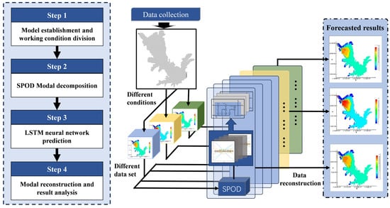 Figure 1. Technical schematic.
2.2. Simulating the Water Quality Concentration Field
This study employs the EFDC model to simulate the spatiotemporal evolution characteristics of the water quality concentration field under various operational scenarios in the study area. Developed by Hamrick at the Virginia Institute of Marine Science, the EFDC model includes multiple hydrological and water quality modules, such as hydrodynamics, water quality, pollutant transport, and sediment transport modules [29]. The EFDC model has been successfully applied in various research areas, including sediment transport, pollutant dynamics, algal blooms, and thermal stratification [30].
The EFDC model applies curvilinear orthogonal coordinate transformation in the horizontal direction and σ coordinate transformation in the vertical direction. The governing equations of the model are as follows [31]:
Continuity equation:
Momentum equation:
State equation:
Concentration transport equation:
In the model, curvilinear orthogonal coordinates are applied horizontally, whereas coordinates are applied vertically: , where ranges from 0 to 1, represents the actual vertical coordinate before the transformation, represents the total depth, represents the bed elevation, and represents the free surface elevation. The velocity components in the curvilinear orthogonal coordinate system for the x and y directions are and , respectively, whereas represents the vertical velocity in the coordinate system. The coefficients , , and are the Jacobian terms for the curvilinear orthogonal coordinate transformation, with . represents the density of the water body; represents the reference density; S represents the salinity; represents the relative hydrostatic pressure; represents the Coriolis force parameter; and represents the vertical turbulent viscosity coefficient. and represent the momentum source and sink terms, respectively, whereas is the vertical turbulent diffusion coefficient. is a source–sink term for a given water quality constituent with concentration .
In this study, the EFDC model was used to develop a two-dimensional hydrodynamic model of the study area. The model topography is built, the grid is divided on the basis of the geographic information of the study area, and three scenarios with different boundary conditions are designed. To simulate various pollutant diffusion scenarios, dye tracers are used instead of traditional water quality indicators, which increases the model’s generality and simplifies the simulation process of pollutant behavior. The output data of the EFDC model are converted into time series snapshots, which are then input into the SPOD model to extract the dynamic modes of the water body.
2.3. SPOD Modal Decomposition
As an extension of the traditional POD method, the SPOD approach is capable of handling both temporal and spatial resolution data, demonstrating several notable advantages [32]. The SPOD method employed in this study is based on the Welch method [33], which uses the batch SPOD algorithm to decompose the dataset [34]. Further derivation formulas can be found in the works of O.T. Schmidt et al. [35], Aaron T. et al. [36], and A. Lario et al. [37].
For concentration field simulations, the output from the EFDC model consists of two-dimensional time series data, which must be reorganized into a time snapshot matrix in the following format:
In this expression, represents the two-dimensional concentration field data, where denotes the number of snapshots, and the spatial coordinate contains available spatial grid points. is the product of the number of spatial grid points and the number of variables , i.e., .
Using the Welch method, the data are divided into segments, yielding overlapping block matrices as follows:
where represents the number of segments, is the number of snapshots per segment, and is the number of overlapping snapshots between segments.
A fast Fourier transform (FFT) is applied to the segmented matrix, yielding:
To reduce spectral leakage, a Hamming window is applied to each segment during the Fourier transform:
The block matrices after the Fourier transform are sorted by frequency in descending order, resulting in a matrix for the -th frequency:
The SPOD modes and their corresponding energies are the eigenvectors and eigenvalues, respectively, of the covariance matrix . The SPOD modes for each frequency are then combined to form:
where is the total number of frequencies, given by .
2.4. Construction of the SPOD Latent Space
The SPOD latent space is composed of the expansion coefficient matrix . After the set of SPOD modes is obtained, the weighted oblique projection method can be employed to derive the expansion coefficient matrix as . This can be expressed as:
In this expression, represents the expansion coefficient matrix with dimensions ; is the SPOD mode matrix sorted by frequency with dimensions ; is the spatial weighting matrix, which defines the inner product space; and is the snapshot matrix of the concentration field.
2.5. Concentration Field Prediction and Reconstruction
The expansion coefficient matrix represents the time-varying intensity and phase of each mode derived from the SPOD method, encapsulating the dynamic characteristics of the temporal evolution of the concentration field. In this study, an LSTM neural network, which is specifically designed to handle sequence data with complex temporal dependencies [38], is employed to predict the expansion coefficient matrix . The structure of the neural network is depicted in Figure 2. The network architecture consists of an input gate, forget gate, output gate, memory cell, and hidden layer. The core algorithm is as follows:
Here, represents the input layer; is the forget gate; is the input gate; denotes the cell state; is the output gate; and is the output of the hidden layer. The matrices are the weight coefficient matrices (e.g., denotes the weight matrix from the input layer to the forget gate), whereas represents the bias vectors (e.g., denotes the bias vector for the forget gate). The function refers to the hyperbolic tangent activation function, and is the sigmoid activation function.
The expansion coefficient matrix obtained through SPOD decomposition is used as input data for the LSTM neural network. The predicted results are subsequently used to reconstruct the concentration field at future time steps, as expressed by the following equation:
In this equation, represents the mode matrix, is the predicted expansion coefficient at time , and is the reconstructed concentration field at time .

Figure 2.
Structure of the LSTM neural network.
3. Case Studies
3.1. Overview of the Study Area
This study selects the Wendegen Reservoir, which is located in the northeastern part of the Inner Mongolia Autonomous Region, China, as the case study area. The Wendegen Reservoir serves as the source reservoir for the Yinchao–Jiliao Water Diversion Project, the largest water diversion project in Inner Mongolia. The reservoir has a normal storage level of 377.00 m, a total storage capacity of 1.964 billion m3, a regulating storage capacity of 1.518 billion m3, and a maximum discharge capacity of 8060 m3/s; the designed water diversion flow rate is 18.58 m3/s. The maximum heights of the main and auxiliary dams are 48.00 m and 14.00 m, respectively. On the basis of the topographical data of the reservoir area, a structured grid was divided with an average grid size of 100 m by 100 m, resulting in a total of 11,267 grids. The model boundary conditions were set as the inflow boundary at the upstream river inlet and the outflow boundary at the dam site. The concentration inlet boundary was placed at the upstream river inlet, as depicted in Figure 3.
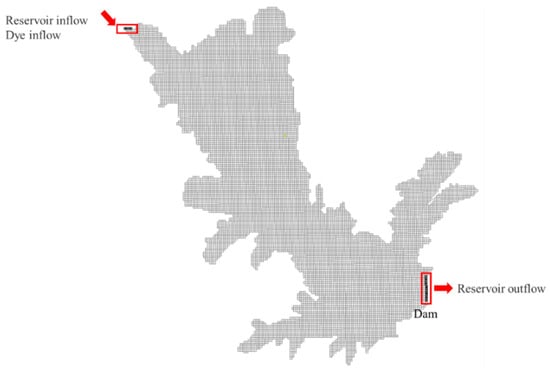
Figure 3.
Model grid division and boundary condition settings.
3.2. Scenario Design
The simulations were conducted via the EFDC model. To increase the model’s versatility while reducing complexity, a dye was selected as a surrogate water quality indicator. The initial dye concentration was set at 10 mg/L, with a degradation coefficient of 0.02, and the reservoir water level was maintained at 375 m. This approach enables a more accurate representation of sedimentation and dispersion processes in natural water bodies.
To assess the applicability of the AI-based water quality model under varying conditions—such as inflow–outflow balance, inflow–outflow imbalance, constant pollutant discharge concentration, and variable pollutant discharge concentration—three computational scenarios were designed, as outlined in Table 1. The pollutant inflow location was consistently set at the reservoir’s inflow point, with a model time step of 1 h, simulating pollutant dispersion over a continuous 10-day period.

Table 1.
Parameter settings for the simulation scenarios.
The simulation results for Scenarios 1, 2, and 3 are presented in Figure 4, Figure 5 and Figure 6, respectively, showing the dynamic changes in pollutant dispersion and its spatial distribution under different conditions.
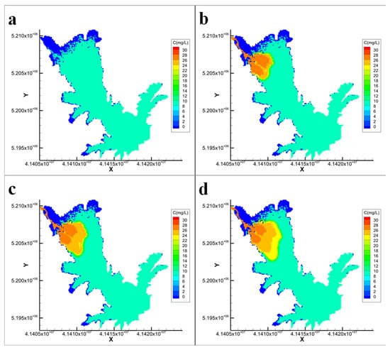
Figure 4.
EFDC model simulation results for Scenario 1 ((a): Day 0; (b): Day 3; (c): Day 6; (d): Day 10; C represents the dye concentration, unit: mg/L).
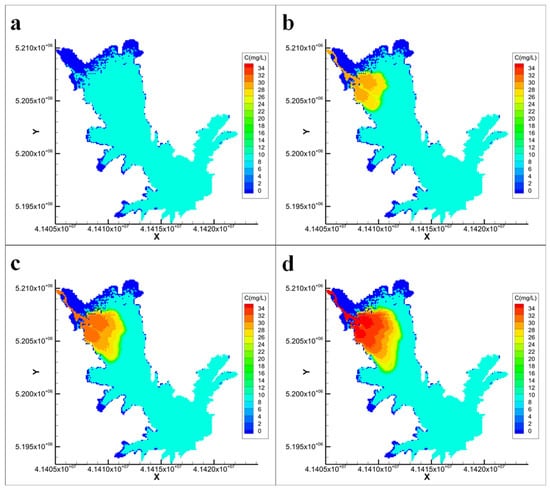
Figure 5.
EFDC model simulation results for Scenario 2 ((a): Day 0; (b): Day 3; (c): Day 6; (d): Day 10; C represents the dye concentration, unit: mg/L).
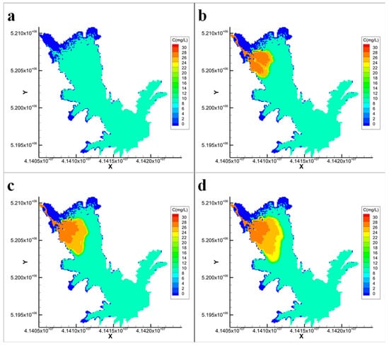
Figure 6.
EFDC model simulation results for Scenario 3 ((a): Day 0; (b): Day 3; (c): Day 6; (d): Day 10; C represents the dye concentration, unit: mg/L).
Compared with the constant condition (Scenario 3), Scenario 1 features a gradual reduction in inflow and outflow rates to half their initial values, whereas the inflow concentration remains constant. A comparison of Figure 4 and Figure 6 reveals that during the initial diffusion period (days 0–3), the reduction in the flow rate had a minimal effect on the pollutant distribution. However, as diffusion continued, the reduction had a significant effect, resulting in higher pollutant concentrations being concentrated near the reservoir inlet. This leads to a more uneven concentration distribution compared with the constant condition, accompanied by a smaller concentration gradient. In Scenario 2, where the inflow and outflow rates remain constant but the pollutant inflow concentration increases over time, a comparison between Figure 5 and Figure 6 demonstrates that the increasing inflow concentration significantly impacts the concentration distribution. During the later stages of dispersion (days 6–10), the extent of the diffusion zone remained largely the same; however, the concentration was notably higher, resulting in a greater concentration gradient. Furthermore, a comparison of Figure 4 and Figure 5 reveals that changes in the pollutant concentration, rather than changes in the flow rate, were the primary factors affecting the concentration field distribution.
3.3. Dataset Composition and Modal Decomposition
Using the EFDC simulation results, concentration field snapshots were obtained for 10 days, totaling 240 h. To avoid the effects of model initialization, data from the first 100 h were discarded. The period from hours 101 to 200, representing the latter phase of concentration diffusion, was selected to form a sampling dataset of length 100 as the initial dataset. The final 40 h, from hours 201 to 240, were retained as a validation set for comparison with the prediction results and assessment of model performance.
To study the effects of different time series input lengths on model prediction accuracy, five sampling datasets were formed using the final 20, 40, 60, 80, and 100 h of the initial dataset. Each dataset was used as input for 12 h lead time concentration field predictions to analyze the prediction error across different sampling dataset sizes. By constructing sampling datasets of varying lengths, this study aimed to comprehensively evaluate the model’s predictive capabilities under diverse data conditions, highlighting its adaptability and robustness in different scenarios.
The use of different numbers of snapshot data for SPOD resulted in varying numbers of modes, as shown in Figure 7. The number of modes obtained increased linearly with the amount of data used. Even with 100 h of snapshot data, the number of modes reached only 49. Therefore, this study adopted full-mode retention and reconstruction techniques, comprehensively considering the dynamic contributions of all modes to enhance the model’s adaptability to nonlinear and complex dynamics, thereby establishing an equivalent full-order prediction mode.
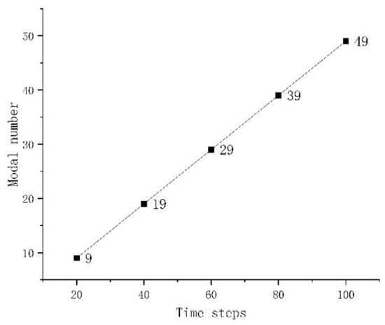
Figure 7.
Number of modes decomposed using different quantities of snapshot data.
Using 20 concentration field snapshots from Scenario 2 as an example, a three-dimensional matrix C(20,174,394) was formed as the input data for SPOD. SPOD was then performed on the input concentration matrix, with the Fourier transform window size set to n_dft = 4, the block overlap rate to l_ovlp = 50%, and the number of blocks to n_blk = 9. Figure 8 shows the spectral energy plot from the SPOD, yielding nine modes, Mode 1 to Mode 9. The energy of Mode 1 and Mode 2 is significantly higher than that of the remaining modes. Mode 1 maintains a consistently high energy level across the entire frequency range, whereas Mode 2 presents slightly lower but relatively stable energy, indicating that these two modes play a dominant role in capturing the primary characteristics of the concentration field. The energy distributions of Modes 3 through 9 decrease gradually, with the energy dropping sharply in the high-frequency range. This suggests that these modes primarily capture secondary features and details in the concentration field, with a greater contribution in the lower frequency range.
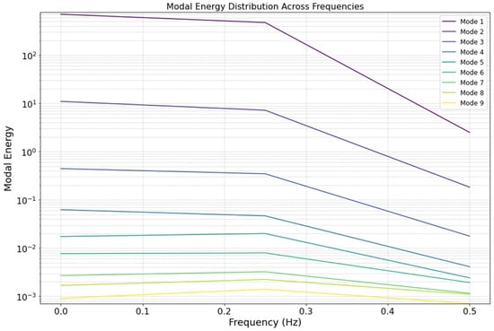
Figure 8.
SPOD energy spectrum at the logarithmic scale for 20 snapshot data points in Scenario 2.
The energy of all the modes decreases to varying degrees as the frequency increases, indicating that high-frequency information is less significant, with the primary features concentrated in the low-frequency range. The principal modes (Modes 1 and 2) are crucial in describing the main dynamic features of the system, whereas the secondary modes (Modes 3 through 9) contain minor physical processes and local information, potentially including noise, disturbances, or small-scale dynamic variations.
4. Results Analysis
The model’s prediction results were evaluated via the coefficient of determination (R2), mean absolute error (MAE), and mean absolute percentage error (MAPE). These metrics are widely recognized as reliable indicators of model performance, with higher R2 and lower MAE and MAPE values typically reflecting better predictive accuracy. The formulas for these evaluation metrics are as follows [39]:
Coefficient of determination (R2):
where and represent the actual and predicted concentration values at the -th position, respectively; is the number of grid cells; and is the mean of the sample values.
Mean absolute error (MAE):
Mean absolute percentage error (MAPE):
Since the full-mode information was used for reconstruction to establish an equivalent full-order model, the prediction errors are entirely attributed to the LSTM neural network, whereas the errors from the SPOD primarily stem from computer floating-point computation errors. Taking Scenario 2, where 20 snapshots of data were used for modal decomposition and reconstruction, as an example, the mean MAE was 5.79 × 10⁻¹⁶ (Figure 9), and the mean R2 value was 1.0.
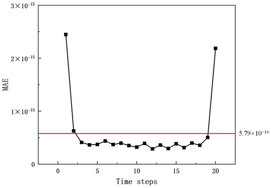
Figure 9.
MAEs for full-mode decomposition and reconstruction of 20 snapshot data points in Scenario 2.
Using the results at the 7th-hour prediction as an example from Scenario 1, where a 60 h sampling dataset was used, Figure 10 compares the model’s prediction with the EFDC simulation results. The model accurately predicts the pollutant dispersion range and trend. In most areas, the prediction results are precise, with significant errors occurring only at the edges where the concentration gradient is steep.
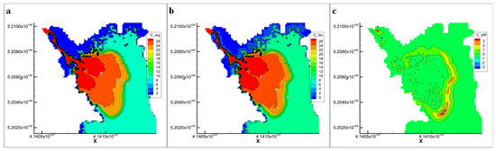
Figure 10.
Prediction results at the 7th hour using a 60 h sampling dataset in Scenario 1 ((a): EFDC Simulation Results, (b): Model Prediction Results, (c): Prediction Error).
4.1. Analysis of the Scenario 1 Prediction Results
For Scenario 1, mode decomposition was performed on each of the five sampling datasets, yielding the corresponding expansion coefficient matrices. Since full-mode information was utilized for modal decomposition and reconstruction, the number of expansion coefficients increased linearly with the length of the time steps (Figure 11), which corresponds to the relationship with the number of modes (Figure 7).

Figure 11.
Relationships between the sampling datasets and the number of expansion coefficients in Scenario 1.
The mode decomposition of the five sampling datasets produced expansion coefficient matrices, which were used as inputs for an LSTM neural network to make predictions iteratively, creating a series of single-input, single-output models for overall prediction. Even with data spanning 100 time steps as input, the data volume for the neural network remains sparse. Therefore, a delay embedding approach was introduced to expand the dataset size and retain the temporal characteristics of the data, thereby improving the efficiency and quality of the neural network model’s learning process.
Given that the initial water concentration was 10 mg/L and that changes in the concentration field are driven primarily by convective diffusion effects due to new pollutant inflows and reservoir flow dynamics, the analysis of the prediction results focuses on two key areas: the diffusion zone where concentrations exceed 10 mg/L and the high-concentration zone where concentrations exceed 20 mg/L. This evaluation aims to assess the model’s prediction accuracy for different levels of pollution and its ability to simulate diffusion effects, thereby enhancing the understanding of pollutant dispersion patterns and model applicability.
Figure 12 presents the evaluation metrics for the diffusion zone and the high-concentration zone. Overall, owing to the iterative multistep prediction method used by the LSTM neural network, the R2 value of the model gradually decreases with increasing prediction time, whereas the MAE and MAPE increase, indicating a decline in prediction accuracy over longer forecast periods and highlighting the model’s limitations for long-term predictions. When a sampling dataset of length 100 was used, the model’s prediction performance was noticeably poorer than that of datasets of length 2080, particularly for the high-concentration zone, where the R2 value decreased to as low as 0.76. This suggests that prediction models built using longer sampling datasets are more complex and have lower generalizability. The increased complexity arises because longer sampling datasets contain more modal information, which increases model complexity while introducing additional noise and redundant information.
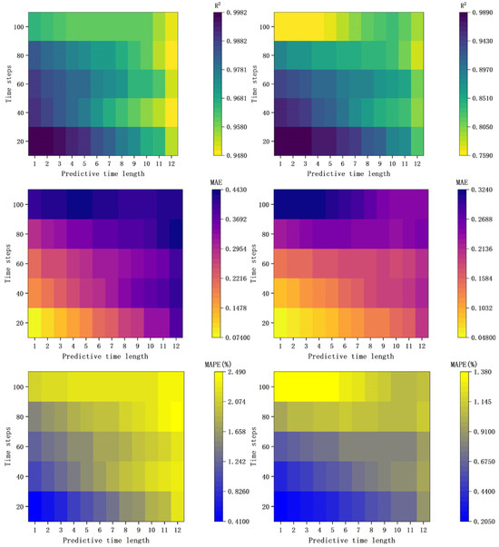
Figure 12.
Evaluation metrics for prediction results in Scenario 1 (First Column: Diffusion Zone Evaluation Metrics; Second Column: High-Concentration Zone Evaluation Metrics).
For the simulation results of the diffusion zone, the model’s prediction performance decreases as the length of the sampling dataset used for prediction increases, particularly for datasets with lengths ranging from 20. This decline in performance is due to the increase in the number of modes as more snapshot data are used, which increases the model’s complexity and makes training more challenging. As shown in Figure 13, the rate of change in all three evaluation metrics decreases with increasing sampling dataset length. Although using a sampling dataset of length 20 yields better short-term prediction results, the prediction errors increase rapidly with longer lead times. On the other hand, models trained with longer sampling datasets exhibit slower changes in prediction errors, indicating that very short sampling datasets are insufficient for capturing the full dynamic information of the concentration field. Moreover, the LSTM-based prediction method cannot ensure accuracy for long lead times when trained on overly short datasets.
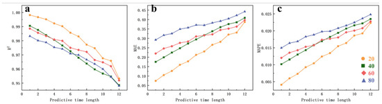
Figure 13.
Trends of the evaluation metrics for the diffusion zone simulation results in Scenario 1 ((a): R2 metric, (b): MAE metric, (c): MAPE metric).
Figure 14 presents the evaluation metrics for the high-concentration zone in Scenario 1. A comparison of Figure 13 and Figure 14 reveals that the trends in the high-concentration zone simulation results are similar to those in the diffusion zone. When shorter sampling datasets are used, the model’s prediction accuracy decreases more noticeably with increasing lead time. For both the diffusion zone and the high-concentration zone, the prediction accuracy decreases as the prediction horizon lengthens, indicating low accuracy for long-term predictions. Although the MAE and MAPE metrics for the high-concentration zone are better than those for the diffusion zone, the R2 metrics for the high-concentration zone are consistently lower than those for the diffusion zone for the same lead time. This indicates that the model’s generalizability is weaker in the high-concentration zone. While the model can simulate the actual value changes in the high-concentration zone relatively well in the short term, the lower R2 reflects a weaker ability to explain data variability in this area.
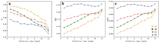
Figure 14.
Trend of evaluation metrics for high-concentration zone simulation results in Scenario 1 ((a): R2 metric, (b): MAE metric, (c): MAPE metric).
4.2. Analysis of the Scenario 2 Prediction Results
Figure 15 shows the evaluation metrics for the prediction results in Scenario 2. Compared with Figure 12, the overall trend in model prediction errors for Scenario 2 is similar to that for Scenario 1. When a sampling dataset of length 100 is used for prediction, the model’s performance is noticeably inferior to that of predictions when datasets of length 20 are used. In Scenario 2, the R2 values for the model using a sampling dataset of length 100 are generally higher than those in Scenario 1, with a minimum R2 value of 0.87 compared with 0.76 in Scenario 1. Although the R2 metric for Scenario 2 is better, the MAE and MAPE metrics are notably worse than those in Scenario 1.
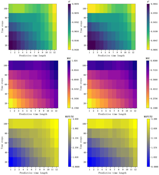
Figure 15.
Evaluation metrics for prediction results in Scenario 2 (First Column: Diffusion Zone Evaluation Metrics; Second Column: High-Concentration Zone Evaluation Metrics).
This difference occurs because, in Scenario 1, the inflow and outflow rates gradually decrease over time while the inflow concentration remains constant, whereas in Scenario 2, the flow rate remains constant while the inflow concentration gradually increases. A comparison of Figure 4 and Figure 5 reveals that higher flow rates and concentrations facilitate pollutant dispersion in both the diffusion zone and the high-concentration zone. The area of the high-concentration zone in Scenario 2 is larger than that in Scenario 1, and the concentration changes are more intense. This makes it harder for the model to capture the changing trends in the concentration field, resulting in poorer generalization for scenarios with more dramatic concentration changes. A comparison of Figure 12 and Figure 15 clearly reveals that for both the diffusion zone and the high-concentration zone, the model prediction performance for Scenario 1 is generally better than that for Scenario 2.
4.3. Analysis of the Scenario 3 Prediction Results
The evaluation metrics for the prediction results of Scenario 3 are presented in Figure 16. By analyzing Figure 12, Figure 15, and Figure 16, the prediction performance of the model for all three scenarios can be comprehensively assessed. For all three scenarios, the model established using a sampling dataset of length 100 consistently produced the worst prediction performance among the corresponding scenarios. This is particularly evident in Scenario 3, where the short-term prediction for the high-concentration zone using the 100-length dataset yielded an R2 value of 0.366.
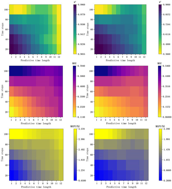
Figure 16.
Evaluation metrics for prediction results in Scenario 3 (First Column: Diffusion Zone Evaluation Metrics; Second Column: High-Concentration Zone Evaluation Metrics).
The primary reason for this is that using a longer sampling dataset for modal decomposition introduces more time series information, which in turn leads to the extraction of more secondary modes and noise. During short-term predictions, the model relies heavily on the most recent modal information, causing these secondary modes and noise to significantly impact the prediction results. Additionally, since Scenario 3 represents a steady-state condition, its concentration field changes more slowly than those of the other two scenarios. As shown in Figure 6, the model shows a more noticeable change in the diffusion zone, whereas changes in the high-concentration zone are relatively slow.
5. Discussion
- Impact of Hydrodynamic Condition Changes on the Prediction Results of the Diffusion Zone.
To examine the impact of changes in reservoir hydrodynamic conditions—caused by reservoir scheduling—on the model’s prediction accuracy, the evaluation metrics for the prediction results from Scenarios 1 and 3 were compared. Figure 17 illustrates the trend of the evaluation metrics for the prediction results in the diffusion zone across both scenarios. The figure clearly shows that for the MAE and MAPE metrics, Scenario 1 outperforms Scenario 3. Additionally, the R2 values in Scenario 1 are consistently higher than those in Scenario 3, further supporting this conclusion. These findings suggest that reservoir scheduling significantly influences the model’s prediction accuracy. Compared with those in Scenario 3, where conditions are less favorable for pollutant dispersion, the pronounced hydrodynamic characteristics in Scenario 1 allow the SPOD method to more accurately capture the primary modal information.
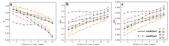
Figure 17.
Comparison of evaluation metric trends for the diffusion zone simulation results between Scenario 1 and Scenario 3 ((a): R2 metric, (b): MAE metric, (c): MAPE metric).
- Impact of Hydrodynamic Conditions on High-concentration Zone Prediction Results.
Figure 18 shows the trends of the evaluation metrics for the prediction results of the high-concentration zones in Scenarios 1 and 3. Compared with Figure 17, although the trends of the three evaluation metrics are similar, the R2 value in Scenario 3 shows a more pronounced decline. This is because, under the steady-state conditions of Scenario 3, pollutant transport in the high-concentration zone is more challenging because of limited convection and diffusion. This finding indicates that the model is more suitable for scenarios with pronounced pollutant dispersion trends. In regions with relatively slow changes, the model struggles to accurately capture the changes in the concentration field, and the noise has a greater influence on the prediction results. The model performs better in scenarios with more dynamic changes.
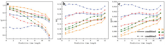
Figure 18.
Comparison of evaluation metric trends for high-concentration zone simulation results between Scenario 1 and Scenario 3 ((a): R2 metric, (b): MAE metric, (c): MAPE metric).
- Impact of Pollutant Inflow Concentration Changes on Pollution Zone Prediction Results.
By comparing the trends in the evaluation metrics for the prediction results of Scenarios 2 and 3 under identical hydrodynamic conditions, the effect of the pollutant inflow concentration on the model’s prediction accuracy can be assessed. A comprehensive comparison of the prediction results from all three scenarios allows us to determine the model’s applicability. Figure 19 shows the trend of the evaluation metrics for the prediction results of the diffusion zone in Scenario 2 and Scenario 3. When combined with the results from Figure 17, the prediction performance when sampling datasets of length 2080 can be analyzed.
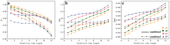
Figure 19.
Comparison of evaluation metric trends for the diffusion zone simulation results between Scenario 2 and Scenario 3 ((a): R2 metric, (b): MAE metric, (c): MAPE metric).
The R2 metric clearly shows that for all three scenarios, there is a significant decline in prediction accuracy for the diffusion zone after 7 h, with the rate of decline also increasing over time. The MAE and MAPE metrics exhibit similar trends, indicating that the model is suitable for short-term water quality predictions (up to 7 h in this case). For longer-term predictions, the accuracy decreases, and the error increases rapidly with increasing lead times. Although using longer windows provides more training data for the neural network, it also introduces more modal information and noise into the modal decomposition process. Therefore, prediction models that are based on long sampling datasets do not outperform those that are based on shorter datasets. In fact, models using shorter sampling datasets achieve similar prediction accuracies with fewer input data, lower model complexity, and shorter training times.
- Impact of Pollutant Inflow Concentration Changes on High-concentration Zone Prediction Results.
By comparing Figure 18 and Figure 20, the model’s simulation performance for the high-concentration zone under different scenarios can be analyzed. Compared with the diffusion zone, the concentration field in the high-concentration zone changes more slowly. In longer sampling datasets, SPOD may extract more low-frequency modes and noise. By analyzing the errors in the high-concentration zone, the model’s accuracy in identifying rapid pollutant dispersion trends can be assessed.
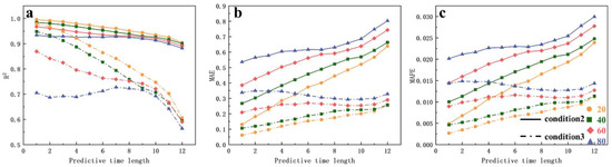
Figure 20.
Comparison of evaluation metric trends for high-concentration zone simulation results between Scenario 2 and Scenario 3 ((a): R2 metric, (b): MAE metric, (c): MAPE metric).
The R2 values for Scenario 3 are significantly lower than those for Scenario 2. This is because Scenario 3 represents a steady-state condition, where pollutant dispersion in the high-concentration zone is very slow, making it difficult for the model to capture its trend. Additionally, longer sampling datasets contain more secondary modes and noise, which is the primary reason for the model’s poorer performance in the high-concentration zone. The trends in the MAE and MAPE for the high-concentration zone are similar to those for the diffusion zone, as the concentration field in the high-concentration zone changes less under steady-state conditions. Although the model’s prediction performance is suboptimal, it does not produce excessively large errors.
Overall, the three evaluation metrics also indicate that the model’s prediction performance decreases after 7 h, suggesting that the model is better suited for short-term water quality prediction, regardless of whether it is used to predict the diffusion zone or the high-concentration zone.
In summary, short sampling datasets are more effective for short-term predictions, as they often provide more accurate results by capturing the concentration field’s variation trends within a specific time period. However, as the length of the training dataset increases, the model may inadvertently incorporate more secondary information and noise, which can reduce prediction accuracy. To mitigate the impact of secondary information, a modal truncation approach can be employed to exclude low-energy modes, thereby optimizing model performance and preserving the critical dynamic features of the concentration field.
- Model performance advantages and future development directions.
The coupled model introduced in this study extends water quality prediction from traditional one-dimensional approaches to two-dimensional fields, enhancing the physical interpretability of the predictions. While achieving a comparable prediction accuracy to conventional deep learning frameworks, it significantly improves the ability to capture dynamic pollutant diffusion processes. Furthermore, compared to traditional machine learning methods such as random forest or XGBoost, the proposed model excels in error control and multidimensional dynamic feature representation, demonstrating greater applicability [40]. This advancement offers an efficient and reliable technical solution for water quality prediction and environmental monitoring. Building on the findings of this study, future research can be expanded in the following directions:
- (1)
- Small sample predictions: In this study, the EFDC simulation results were used as surrogate datasets for modal decomposition. In practical engineering applications, other data sources can be substituted. Since the model itself is suitable for short-term data prediction with certain trends, it can be applied to sudden water pollution incidents. By constructing input datasets using small sample data from real-time emergency and regular monitoring, the model can achieve rapid short-term predictions of pollutant dispersion trends.
- (2)
- Low spatiotemporal resolution prediction: For different water quality indicators, such as chlorophyll, which can be obtained through satellite remote sensing, similar methods can be employed for two-dimensional concentration field predictions. However, satellite remote sensing data often lack both high temporal resolution and high spatial resolution. To address this issue, spatial interpolation methods such as Thiessen polygons (TSNs), inverse distance weighting, multivariate interpolation, and kriging [41], alongside temporal interpolation methods that either treat time as an independent dimension or extend it as a spatial dimension [42], can be employed to enrich datasets. This approach could increase the accuracy and reliability of predictions based on satellite remote sensing data.
- (3)
- Optimization of neural networks and modal decomposition: With the rapid advancement of information technology, increasingly powerful and faster neural networks are continually emerging. Different neural networks may yield varying results when predicting the expansion coefficient matrix, leading to differences in accuracy. Networks such as Informer [43] and Mamba [44] have achieved significant success across various fields. To further increase the model’s speed while ensuring accuracy, high-energy modes can be selectively used for the calculation and reconstruction of the expansion coefficient matrix. However, it should be noted that the number of modes selected must be determined on the basis of user expertise, depending on the specific scenarios and datasets.
- (4)
- Water quality digital twin model: The concept of a digital twin represents a crucial technological pathway for driving the informatization and intelligent development of various industries, including environmental management. As highlighted in this study, the proposed model serves as a foundation for developing a digital twin for water quality by addressing key challenges in managing high-dimensional spatiotemporal data. Using high-fidelity simulations, initial sample sets can be generated to represent concentration field distributions under varying boundary conditions, capturing a broader range of parameters, including those that are challenging or impractical to monitor in real-world scenarios. The integration of modal decomposition, as demonstrated in this study, enables the extraction of dominant dynamic features, while coupling with response surface analysis facilitates the development of a surrogate model. This surrogate model establishes a robust and interpretable relationship between input boundary conditions and output concentration fields. This approach would not only support the preliminary realization of short-term predictions under diverse conditions but also pave the way for scalable, real-time applications in water quality monitoring and sustainable resource management [45].
- (5)
- Model Dimensional Expansion: Although this study focuses on two-dimensional water quality predictions, from a theoretical perspective, the SPOD method is capable of performing modal decomposition on three-dimensional data. However, the complexity of three-dimensional data far exceeds that of two-dimensional data, posing significant challenges to directly establishing a complete prediction model for three-dimensional scalar or vector fields, including issues related to model complexity, computation time, and prediction accuracy. For three-dimensional data, an alternative approach is to slice the dataset into multiple two-dimensional layers. This approach not only helps control the overall model scale but also enables modeling at any arbitrary spatial position, providing a basis for more in-depth investigations.
6. Conclusions
This study integrates spectral proper orthogonal decomposition (SPOD) with long short-term memory (LSTM) neural networks to address challenges in managing high-dimensional spatiotemporal water quality data. By combining physical interpretability with data-driven modeling, the proposed method achieves efficient and accurate predictions while capturing pollutant diffusion dynamics under varying conditions. This model provides practical value for environmental management, including rapid responses to pollution events and optimized reservoir operations, and lays the groundwork for developing digital twin systems for real-time water quality monitoring and sustainable resource management.
By using SPOD for modal decomposition to construct a latent space, the dimensionality of the two-dimensional concentration field time series data is reduced, enabling efficient prediction via neural networks, followed by reconstruction back to the high-dimensional data. The proposed method not only advances surrogate modeling techniques but also offers practical applications for environmental management and pollution control, laying a foundation for the future development of digital twin systems in water quality monitoring. The three typical scenarios presented in this paper encompass situations that may be encountered in practical engineering applications or transitional states between different conditions. By analyzing the model’s performance under these scenarios, the following conclusions can be drawn:
- (1)
- For the three scenarios presented in this paper, it is concluded that using sampling datasets of lengths between 20 and 80 h for prediction within 7 h yields good model performance.
- (2)
- The two-dimensional short-term water quality prediction model based on SPOD and LSTM generally has high accuracy. For overall model prediction, in Scenario 1, four sampling dataset lengths (20, 40, 60, and 80) resulted in an average R2 of 0.93, an average MAE of 0.24, and an average MAPE of 1.22%. Scenario 2, with the same sampling dataset length, achieved an average R2 of 0.96, an average MAE of 0.58, and an average MAPE of 2.48%. Scenario 3, which uses four sampling dataset lengths, yielded an average R2 of 0.86, an average MAE of 0.32, and an average MAPE of 1.61%. The model can accurately capture pollutant concentration changes and diffusion trends.
- (3)
- A physically interpretable two-dimensional water quality prediction neural network model was explored. Compared with traditional neural network-based water quality prediction models, this model increases prediction dimensionality while ensuring accuracy, allowing for the effective prediction of changes in two-dimensional water quality concentration fields. Additionally, the dataset derived from physical governing equations effectively enhances the interpretability of the neural network model. The model can also be extended to predict other two-dimensional scalar fields.
Author Contributions
Conceptualization, S.Z. and J.L.; methodology, S.Z.; software, S.Z.; validation, Y.L., D.Z. and J.L.; formal analysis, S.Z.; investigation, B.Z.; resources, B.Z.; data curation, T.J.; writing—original draft preparation, S.Z.; writing—review and editing, J.L.; visualization, B.Z.; supervision, D.Z.; project administration, Q.P.; funding acquisition, Q.P. All authors have read and agreed to the published version of the manuscript.
Funding
This research was funded by the Research Project of China Yangtze Power Company Limited, grant number Z242302042, and the Hubei Provincial Natural Science Foundation Project, grant number 2024AFD356, and the Major Science and Technology Project of the Ministry of Water Resources, P.R.C., grant number SKS-2022117.
Institutional Review Board Statement
Not applicable.
Informed Consent Statement
Not applicable.
Data Availability Statement
Data from the study are available upon request.
Conflicts of Interest
The authors declare no conflicts of interest.
References
- Vanda, S.; Nikoo, M.R.; Taravatrooy, N.; Sadegh, M.; Al-Wardy, M.; Adamowski, J.F. An emergency multi-objective compromise framework for reservoir operation under suddenly injected pollution. J. Hydrol. 2021, 598, 126242. [Google Scholar] [CrossRef]
- Li, L.; Haoran, Y.; Xiaocang, X. Effects of Water Pollution on Human Health and Disease Heterogeneity: A Review. Front. Environ. Sci. 2022, 10, 880246. [Google Scholar] [CrossRef]
- Huang, Y.; Cai, Y.; He, Y.; Dai, C.; Wan, H.; Guo, H. A water quality prediction approach for the Downstream and Delta of Dongjiang River Basin under the joint effects of water intakes, pollution sources, and climate change. J. Hydrol. 2024, 640, 131686. [Google Scholar] [CrossRef]
- Rangecroft, S.; Dextre, R.M.; Richter, I.; Bueno, C.V.; Kelly, C.; Turin, C.; Fuentealba, B.; Hernandez, M.C.; Morera, S.; Martin, J.; et al. Unravelling and understanding local perceptions of water quality in the Santa basin, Peru. J. Hydrol. 2023, 625, 129949. [Google Scholar] [CrossRef]
- Wu, Z.; Wang, X.; Chen, Y.; Cai, Y.; Deng, J. Assessing river water quality using water quality index in Lake Taihu Basin, China. Sci. Total Environ. 2018, 612, 914–922. [Google Scholar] [CrossRef]
- Nong, X.; Lai, C.; Chen, L.; Shao, D.; Zhang, C.; Liang, J. Prediction modelling framework comparative analysis of dissolved oxygen concentration variations using support vector regression coupled with multiple feature engineering and optimization methods: A case study in China. Ecol. Indic. 2023, 146, 109845. [Google Scholar] [CrossRef]
- Gai, R.; Zhang, H. Prediction model of agricultural water quality based on optimized logistic regression algorithm. EURASIP J. Adv. Signal Process. 2023, 2023, 21. [Google Scholar] [CrossRef]
- Tebebal, M.E. Overview of water quality modeling. Cogent Eng. 2021, 8, 1891711. [Google Scholar]
- Qiu, C.; Wan, Y. Time series modeling and prediction of salinity in the Caloosahatchee River Estuary. Water Resour. Res. 2013, 49, 5804–5816. [Google Scholar] [CrossRef]
- Tiyasha Tung, T.M.; Yaseen, Z.M. A survey on river water quality modelling using artificial intelligence models: 2000–2020. J. Hydrol. 2020, 585, 124670. [Google Scholar] [CrossRef]
- Wang, Q.; Li, Z.; Cai, J.; Zhang, M.; Liu, Z.; Xu, Y.; Li, R. Spatially adaptive machine learning models for predicting water quality in Hong Kong. J. Hydrol. 2023, 622, 129649. [Google Scholar] [CrossRef]
- Wang, Z.; Duan, L.; Shuai, D.; Qiu, T. Research on water environmental indicators prediction method based on EEMD decomposition with CNN-BiLSTM. Sci. Rep. 2024, 14, 1676. [Google Scholar] [CrossRef] [PubMed]
- Elkiran, G.; Nourani, V.; Abba, S. Multi-step ahead modelling of river water quality parameters using ensemble artificial intelligence-based approach. J. Hydrol. 2019, 577, 123962. [Google Scholar] [CrossRef]
- Wan, H.; Xu, R.; Zhang, M.; Cai, Y.; Li, J.; Shen, X. A novel model for water quality prediction caused by non-point sources pollution based on deep learning and feature extraction methods. J. Hydrol. 2022, 612, 128081. [Google Scholar] [CrossRef]
- Tripathy, P.K.; Mishra, K.A. Deep learning in hydrology and water resources disciplines: Concepts, methods, applications, and research directions. J. Hydrol. 2024, 628, 130458. [Google Scholar] [CrossRef]
- Lui HF, S.; Wolf, W.R. Construction of reduced-order models for fluid flows using deep feedforward neural networks. J. Fluid Mech. 2020, 872, 963–994. [Google Scholar] [CrossRef]
- Eivazi, H.; Veisi, H.; Naderi, M.H.; Esfahanian, V. Deep Neural Networks for Nonlinear Model Order Reduction of Unsteady Flows. Phys. Fluids 2020, 32, 105104. [Google Scholar] [CrossRef]
- Wu, P.; Sun, J.; Chang, X.; Zhang, W.; Arcucci, R.; Guo, Y.; Pain, C.C. Data-driven reduced order model with temporal convolutional neural network. Comput. Methods Appl. Mech. Eng. 2020, 360, 112766. [Google Scholar] [CrossRef]
- Burkardt, J.; Gunzburger, M.; Lee, H. POD and CVT-based reduced-order modeling of Navier–Stokes flows. Comput. Methods Appl. Mech. Eng. 2006, 196, 337–355. [Google Scholar] [CrossRef]
- SCHMIDJ, P. Dynamic mode decomposition of numerical and experimental data. J. Fluid Mech. 2010, 656, 5–28. [Google Scholar] [CrossRef]
- Long, Y.; Guo, X.; Xiao, T. Research, Application and Future Prospect of Mode Decomposition in Fluid Mechanics. Symmetry 2024, 16, 155. [Google Scholar] [CrossRef]
- Zhang, B.; Ooka, R.; Kikumoto, H. Analysis of turbulent structures around a rectangular prism building model using spectral proper orthogonal decomposition. J. Wind Eng. Ind. Aerodyn. 2020, 206, 104213. [Google Scholar] [CrossRef]
- Schmidt, O.T. Spectral proper orthogonal decomposition using multitaper estimates. Theor. Comput. Fluid Dyn. 2022, 36, 741–754. [Google Scholar] [CrossRef]
- He, J.; Chen, Z.; Zhao, C.; Chen, X.; Wei, Y.; Zhang, C. Wave Parameter Inversion With Coherent Microwave Radar Using Spectral Proper Orthogonal Decomposition. IEEE Trans. Geosci. Remote Sens. 2022, 60, 3203512. [Google Scholar] [CrossRef]
- Fiore, M.; Gojon, R.; Sáez-Mischlich, G.; Gressier, J. LES of the T 106 low-pressure turbine: Spectral proper orthogonal decomposition of the flow based on a fluctuating energy norm. Comput. Fluids 2023, 252, 105761. [Google Scholar] [CrossRef]
- Zhang, B.; Ooka, R.; Kikumoto, H. Spectral Proper Orthogonal Decomposition Analysis of Turbulent Flow in a Two-Dimensional Street Canyon and Its Role in Pollutant Removal. Bound.-Layer Meteorol. 2022, 183, 97–123. [Google Scholar] [CrossRef]
- Zeng, X.; Zhang, Y.; He, C.; Liu, Y. Time- and frequency-domain spectral proper orthogonal decomposition of a swirling jet by tomographic particle image velocimetry. Exp. Fluids Exp. Methods Their Appl. Fluid Flow 2023, 64, 5. [Google Scholar] [CrossRef]
- Li, X.B.; Chen, G.; Liang, X.F.; Liu, D.R.; Xiong, X.H. Research on spectral estimation parameters for application of spectral proper orthogonal decomposition in train wake flows. Phys. Fluids 2021, 33, 125103. [Google Scholar] [CrossRef]
- Peng, S.; Fu, G.Y.; Zhao, X.H.; Moore, B.C. Integration of Environmental Fluid Dynamics Code (EFDC) Model with Geographical Information System (GIS) Platform and Its Applications. J. Environ. Inform. 2011, 17, 75–82. [Google Scholar] [CrossRef]
- Bai, J.; Zhao, J.; Zhang, Z.; Tian, Z. Assessment and a review of research on surface water quality modeling. Ecol. Model. 2022, 466, 109888. [Google Scholar] [CrossRef]
- Ai, H.; Zhang, W.S.; Hu, X.B.; He, Q.; Liu, Y. The Research and Application Progress of Environmental Fluid Dynamics Code. J. Water Resour. Res. 2014, 3, 247–256. [Google Scholar] [CrossRef]
- Sieber, M.; Paschereit, C.O.; Oberleithner, K. Spectral proper orthogonal decomposition. J. Fluid Mech. 2016, 792, 798–828. [Google Scholar] [CrossRef]
- Welch, P.D. The use of fast Fourier transform for the estimation of power spectra: A method based on time averaging over short, modified periodograms. IEEE Trans. Audio Electroacoust. 1967, 15, 70–73. [Google Scholar] [CrossRef]
- Schmidt, O.T.; Towne, A. An efficient streaming algorithm for spectral proper orthogonal decomposition. Comput. Phys. Commun. 2017, 237, 98–109. [Google Scholar] [CrossRef]
- Schmidt, O.T.; Colonius, T. Guide to Spectral Proper Orthogonal Decomposition. AIAA J. 2020, 58, 1023–1033. [Google Scholar] [CrossRef]
- Aaron, T.; Schmidt, O.T.; Tim, C. Spectral proper orthogonal decomposition and its relationship to dynamic mode decomposition and resolvent analysis. J. Fluid Mech. 2017, 847, 821–867. [Google Scholar] [CrossRef]
- Lario, A.; Maulik, R.; Schmidt, O.T.; Rozza, G.; Mengaldo, G. Neural-network learning of SPOD latent dynamics. J. Comput. Phys. 2022, 486, 111475. [Google Scholar] [CrossRef]
- Yu, Y.; Si, X.; Hu, C.; Zhang, J. A Review of Recurrent Neural Networks: LSTM Cells and Network Architectures. Neural Comput. 2019, 31, 1235–1270. [Google Scholar] [CrossRef]
- Butt, F.M.; Hussain, L.; Mahmood, A.; Lone, K.J. Artificial Intelligence based accurately load forecasting system to forecast short and medium-term load demands. Math. Biosci. Eng. 2020, 18, 400–425. [Google Scholar] [CrossRef]
- Singha, S.; Pasupuleti, S.; Singha, S.S.; Singh, R.; Kumar, S. Prediction of groundwater quality using efficient machine learning technique. Chemosphere 2021, 276, 130265. [Google Scholar] [CrossRef]
- Hwang, H.S.; Kim, B.K.; Han, D. Comparison of methods to estimate areal means of short duration rainfalls in small catchments, using rain gauge and radar data. J. Hydrol. 2020, 588, 125084. [Google Scholar] [CrossRef]
- Li, L.; Revesz, P. Interpolation methods for spatio-temporal geographic data. Comput. Environ. Urban Syst. 2004, 28, 201–227. [Google Scholar] [CrossRef]
- Zhou, H.; Zhang, S.; Peng, J.; Zhang, S.; Li, J.; Xiong, H.; Zhang, W. Informer: Beyond Efficient Transformer for Long Sequence Time-Series Forecasting. Proc. AAAI Conf. Artif. Intell. 2020, 35, 11106–11115. [Google Scholar] [CrossRef]
- Gu, A.; Dao, T. Mamba: Linear-time sequence modeling with selective state spaces. arXiv 2023, arXiv:2312.00752. [Google Scholar]
- Liu, Y.; Meng, X.; Hu, L.; Bao, Y.; Hancock, C. Application of Response Surface-Corrected Finite Element Model and Bayesian Neural Networks to Predict the Dynamic Response of Forth Road Bridges under Strong Winds. Sensors 2024, 24, 2091. [Google Scholar] [CrossRef]
Disclaimer/Publisher’s Note: The statements, opinions and data contained in all publications are solely those of the individual author(s) and contributor(s) and not of MDPI and/or the editor(s). MDPI and/or the editor(s) disclaim responsibility for any injury to people or property resulting from any ideas, methods, instructions or products referred to in the content. |
© 2024 by the authors. Licensee MDPI, Basel, Switzerland. This article is an open access article distributed under the terms and conditions of the Creative Commons Attribution (CC BY) license (https://creativecommons.org/licenses/by/4.0/).