
A Dynamic Prediction Framework for Urban Public Space Vitality: From Hypothesis to Algorithm and Verification

Abstract
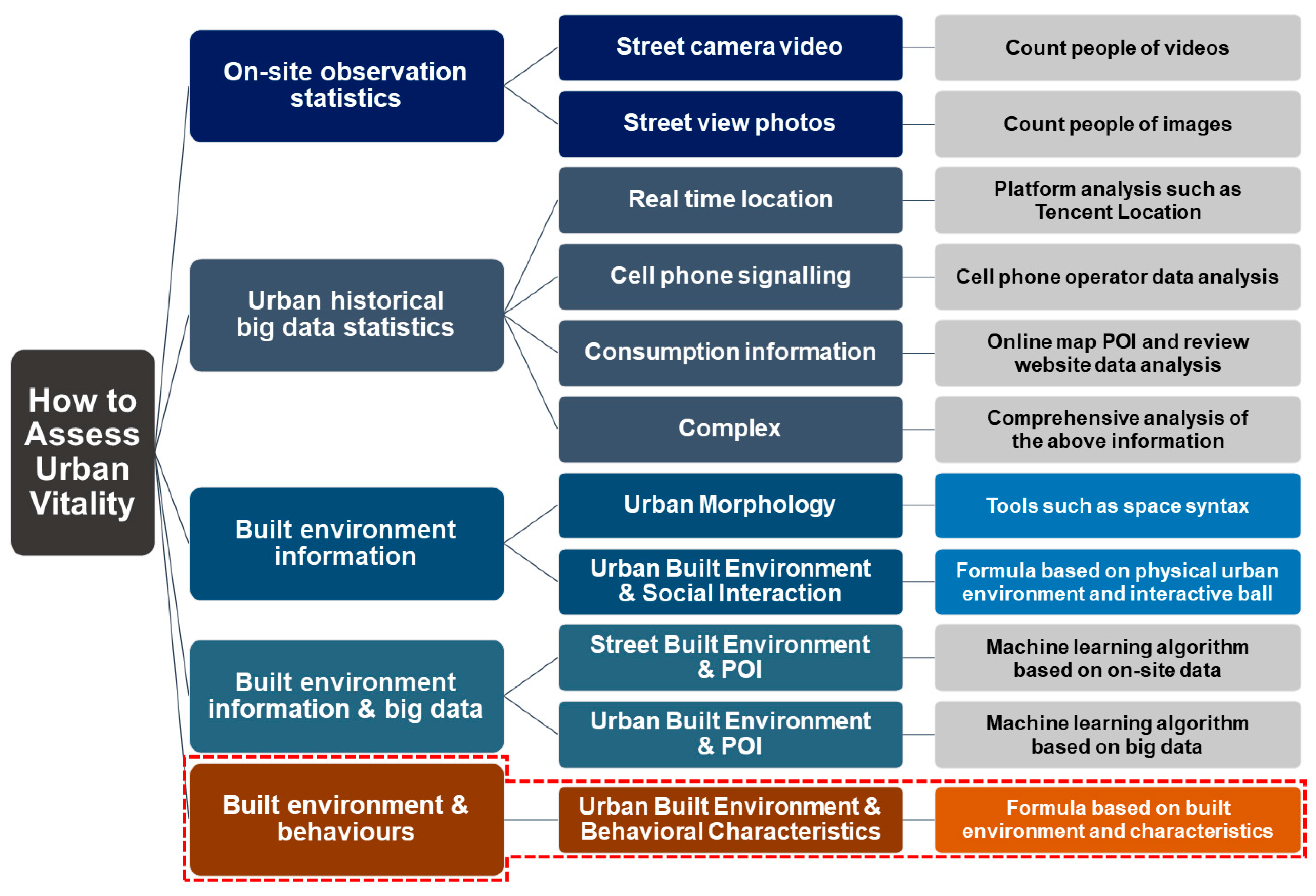
1. Research Background and Introduction
2. Theory of Time Dimension Dynamic Based on Crowd-Frequency
2.1. Hypothesis
- H01: The usage of a space during a particular period is influenced by crowd preferences.
- H02: Specific crowds tend to adhere to predetermined schedules when utilizing urban spaces.
2.2. Specific Parameters
- Crowds
- Frequency
3. Algorithm Construction
3.1. Indicators
3.1.1. Indicator System of Past Studies
3.1.2. New Indicator System
3.2. Algorithm and Formula
4. Prediction Framework Verification and Further Development through a Case Study
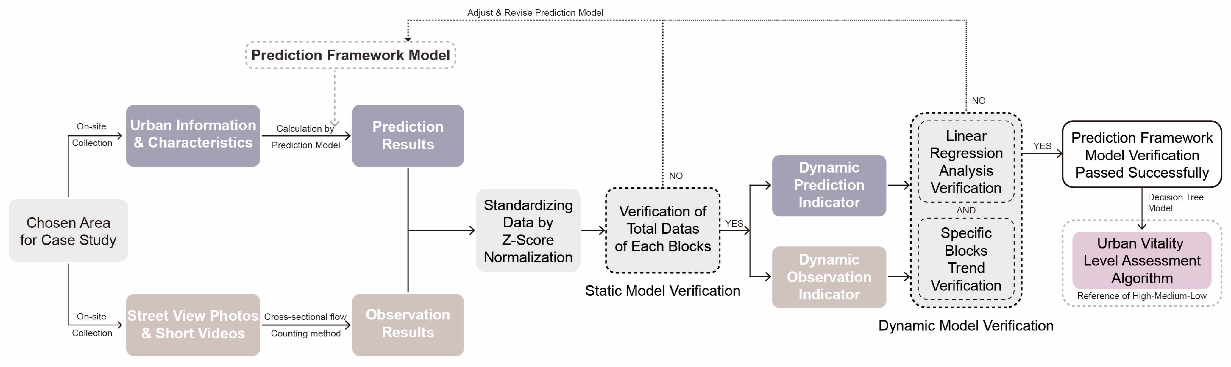
4.1. Verification Flow
4.2. Selection of Case Area for Experimental Verification
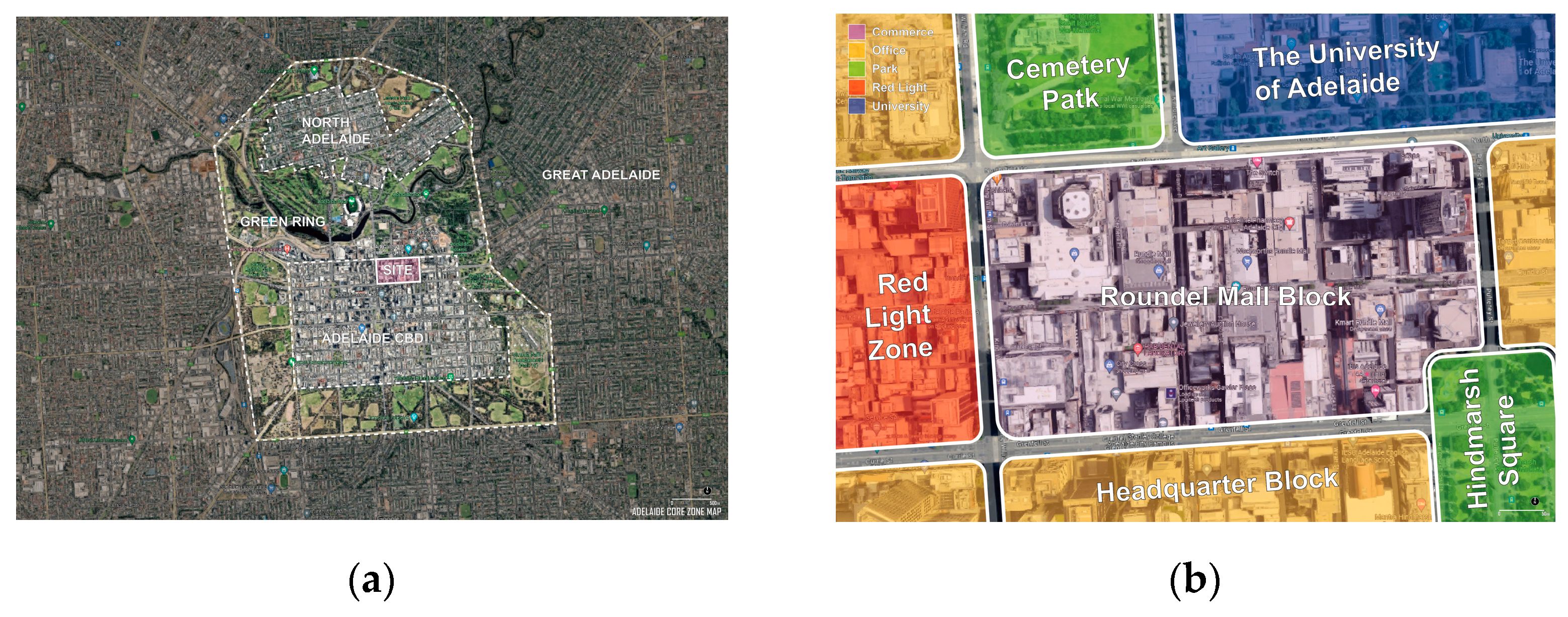
4.2.1. Adelaide Roundel Mall Block
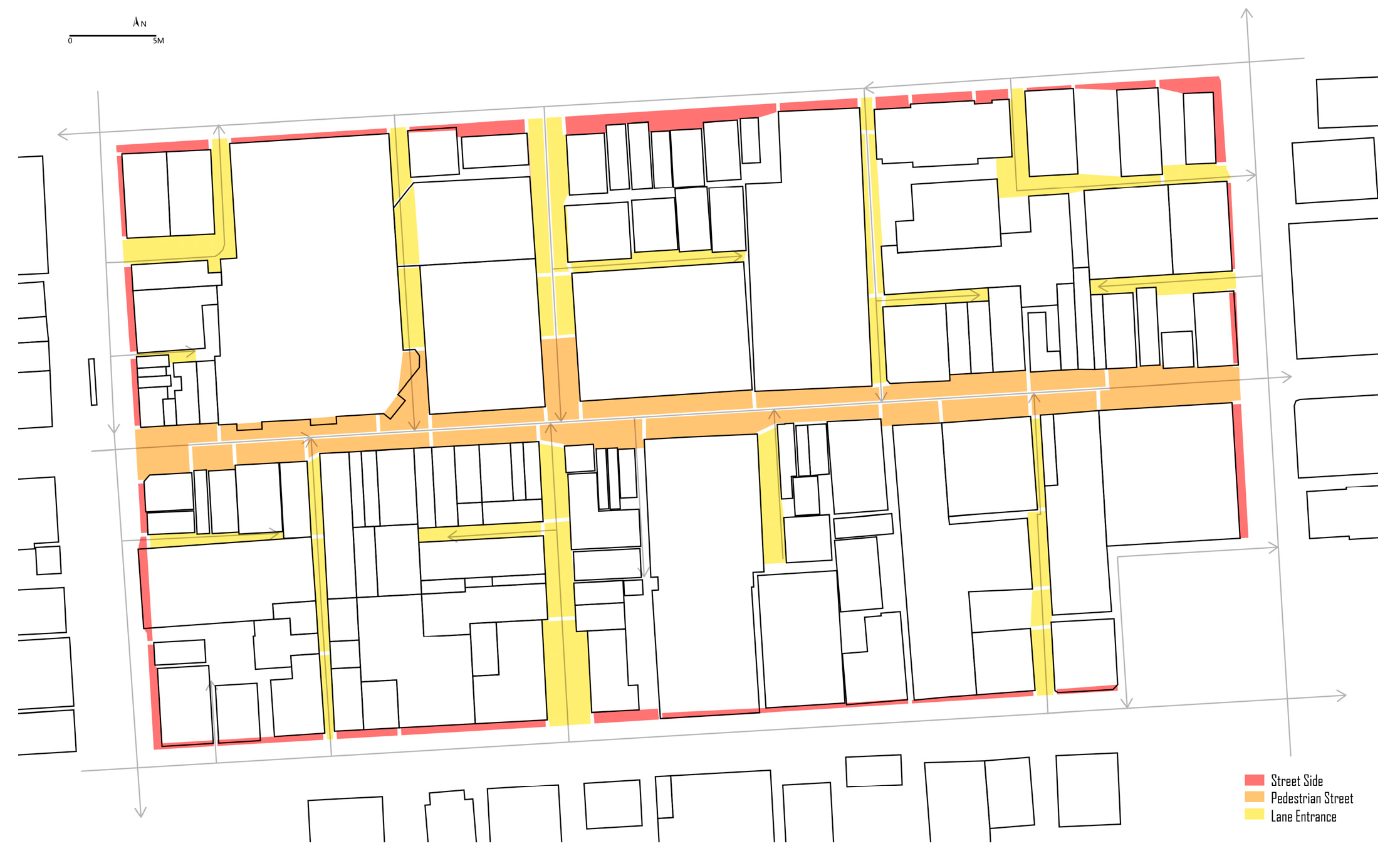
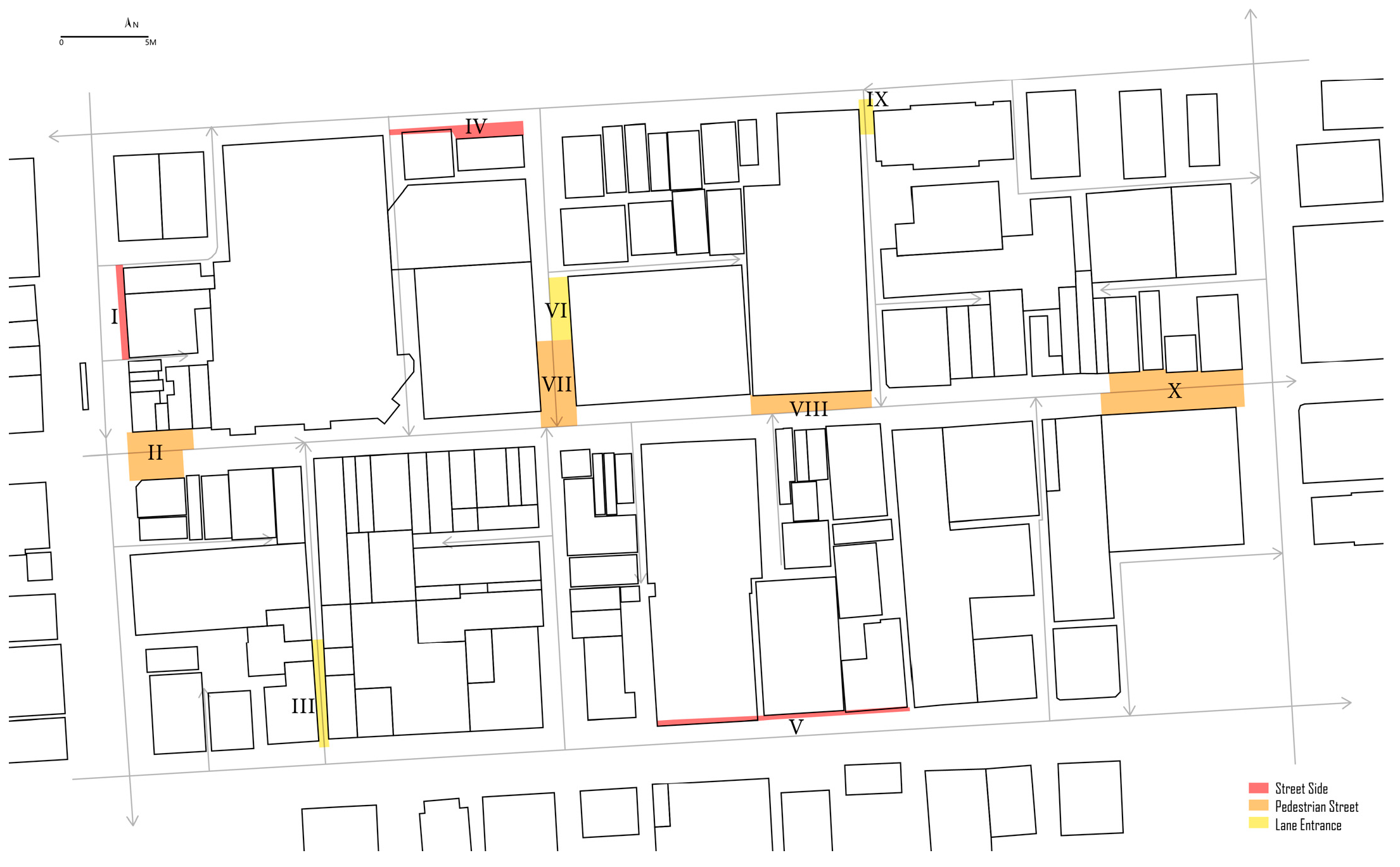
4.2.2. Suite Division and Numbering
4.3. Obtaining and Calculating Each Parameter in the Prediction Model
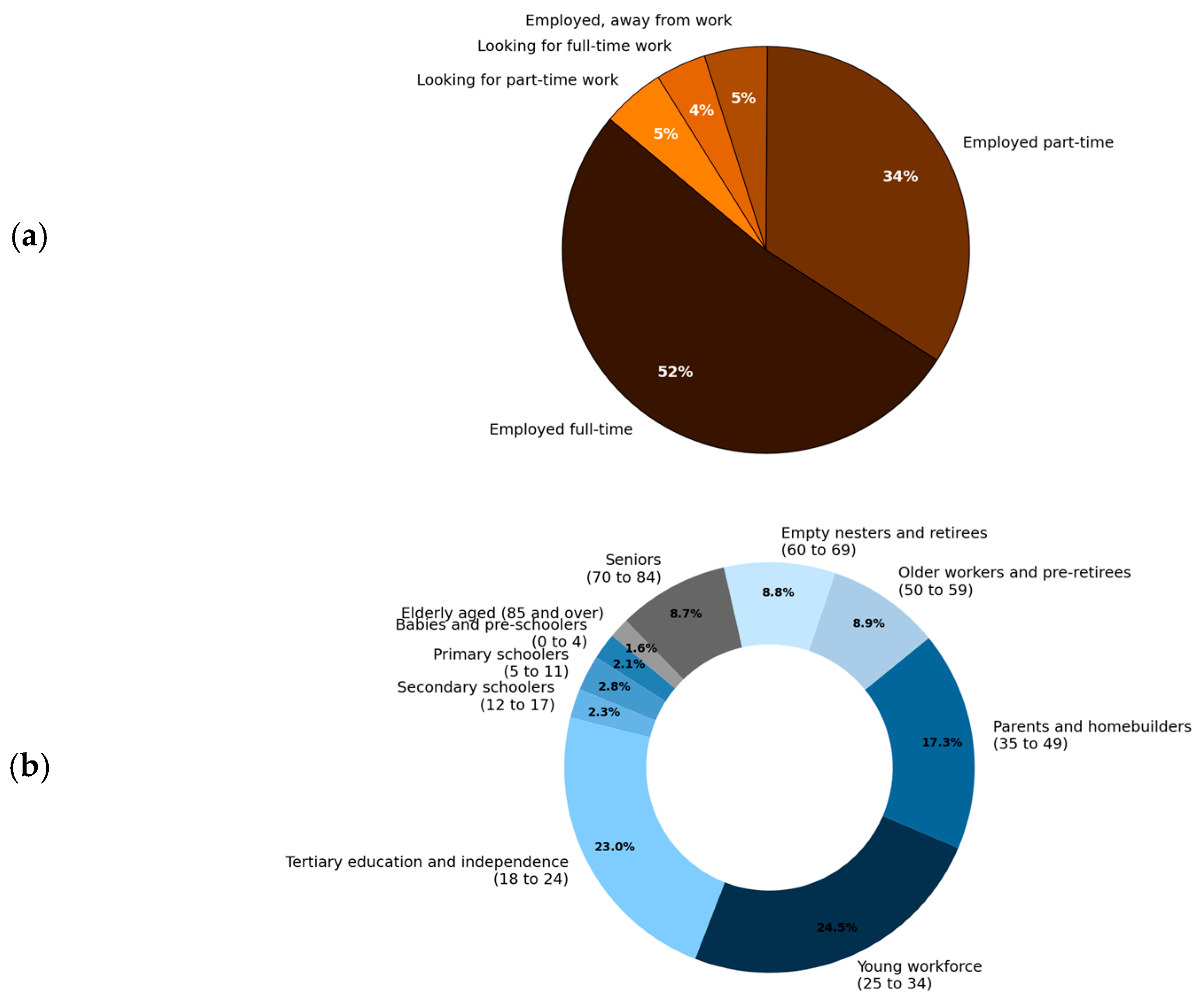
4.3.1. Crowds and Frequency Analysis
4.3.2. Collection of Other Parameters in the Prediction Model
- Area—functional area. The results are obtained by counting the building area and site area in each spatial unit.
- Space access coefficient—assigned based on the openness of each functional space inside and outside the space unit. Completely free is 4, quasi-free opening requirement is 3, potential consumption requirement is 2, fully charged is 1.
- Interaction coefficient—mainly determined based on the land use properties of the space unit, combined with the functional characteristics of indoor and outdoor spaces to assist judgment, and finally determined based on the interactive sphere model.
- Attraction coefficient—determined by the type and level of landscape/activities in the space. According to the location and scale of the attraction point, assign values from 0 to 3, respectively. The higher the value, the greater the influence.
- Auto accessibility—comprehensive calculation based on the distance to public transportation stops. There are nine bus stations, and three train stations around the research plot.
- Walking accessibility—comprehensive calculation of walkable area.
- NEG—spatial external negative factors. First, conduct on-site research to determine the number of negative impact points in the site and make statistics. A large trash can is worth 1, a small trash can is worth 0.5, and a homeless person is worth 1. Then the negative records of each spatial unit are accumulated and obtained.
4.4. Field Observation Data Collection and Processing
4.5. Data Analysis and Comparison Verification
4.5.1. Static Model Results Validation
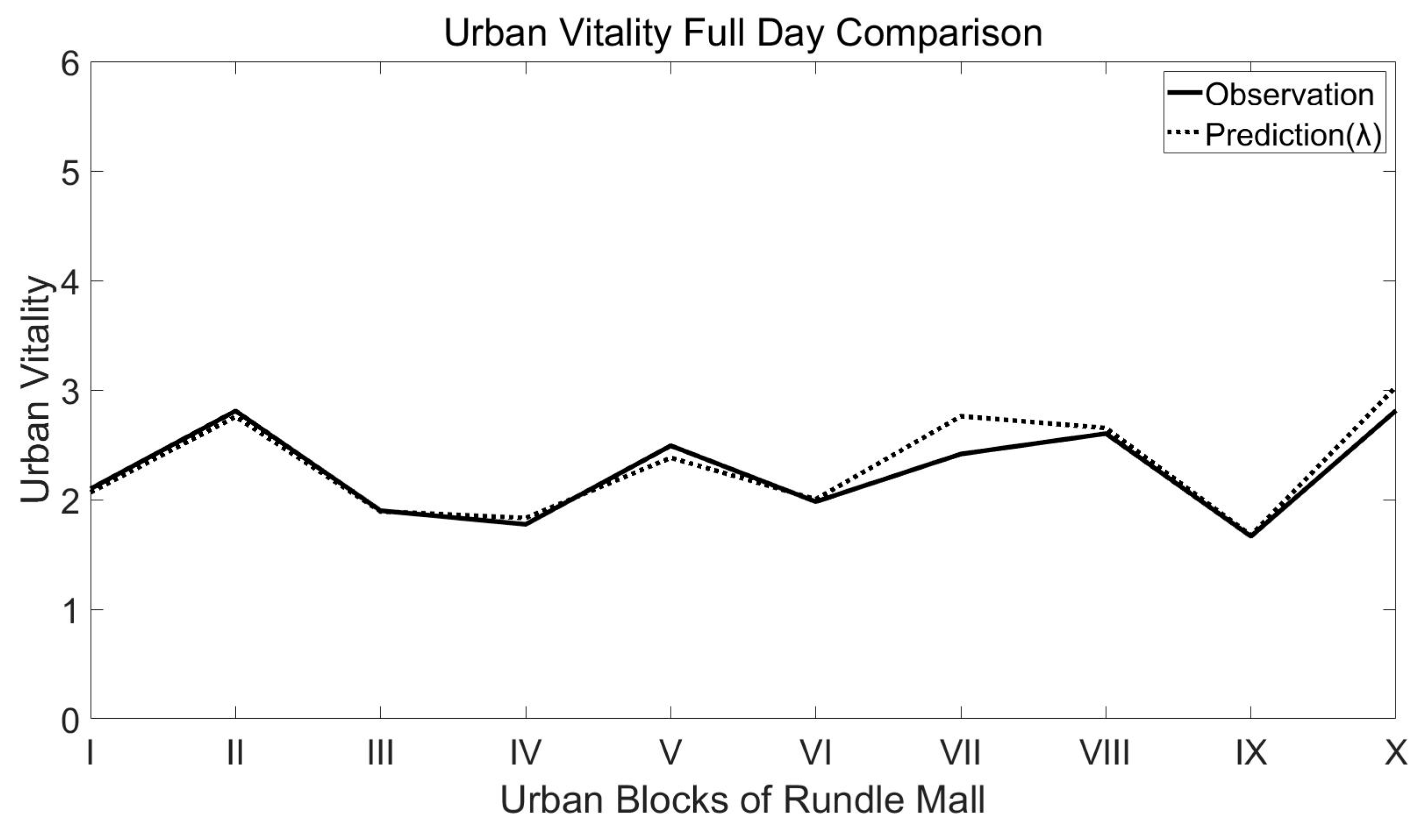
4.5.2. Dynamic Model Results Validation
4.6. A Preliminary Vitality Level Prediction Program Based on Decision Tree Model
5. Discussion
6. Conclusions
Author Contributions
Funding
Institutional Review Board Statement
Informed Consent Statement
Data Availability Statement
Conflicts of Interest
References
- Moser, S. Forest city, Malaysia, and Chinese expansionism. Urban Geogr. 2018, 39, 935–943. [Google Scholar] [CrossRef]
- Shi, L.; Wurm, M.; Huang, X.; Zhong, T.; Leichtle, T.; Taubenböck, H. Urbanization that Hides in the Dark—Spotting China’s “Ghost Neighborhoods” from Space. Landsc. Urban Plan. 2020, 200, 103822. [Google Scholar] [CrossRef]
- Chen, K. Ghost Cities of China. The Story of Cities without People in the World’s Most Populated Country. Eur. Stud. 2017, 69, 998–999. [Google Scholar] [CrossRef]
- Wang, J.; Yang, Z.; Qian, X. Driving Factors of Urban Shrinkage: Examining the Role of Local Industrial Diversity. Cities 2020, 99, 102646. [Google Scholar] [CrossRef]
- Yang, Z.; Pan, Y. Are Cities Losing Their Vitality? Exploring Human Capital in Chinese Cities. Habitat Int. 2020, 96, 102104. [Google Scholar] [CrossRef]
- Jacobs, J. The Death and Life of Great American Cities. 1961; Vintage: New York, NY, USA, 1992; pp. 321–325. [Google Scholar]
- Montgomery, J. Making a City: Urbanity, Vitality and Urban Design. J. Urban Des. 1998, 3, 93–116. [Google Scholar] [CrossRef]
- Chen, W.; Wu, A.N.; Biljecki, F. Classification of Urban Morphology with Deep Learning: Application on Urban Vitality. Comput. Environ. Urban Syst. 2021, 90, 101706. [Google Scholar] [CrossRef]
- Liu, H.; Gou, P.; Xiong, J. Vital Triangle: A New Concept to Evaluate Urban Vitality. Comput. Environ. Urban Syst. 2022, 98, 101886. [Google Scholar] [CrossRef]
- Xu, Y.; Chen, X. Quantitative Analysis of Spatial Vitality and Spatial Characteristics of Urban Underground Space (UUS) in Metro Area. Tunn. Undergr. Space Technol. 2021, 111, 103875. [Google Scholar] [CrossRef]
- Chen, Y.; Yu, B.; Shu, B.; Yang, L.; Wang, R. Exploring the Spatiotemporal Patterns and Correlates of Urban Vitality: Temporal and Spatial Heterogeneity. Sustain. Cities Soc. 2023, 91, 104440. [Google Scholar] [CrossRef]
- Lv, G.; Zheng, S.; Hu, W. Exploring the relationship between the built environment and block vitality based on multi-source big data: An analysis in Shenzhen, China. Geomat. Nat. Hazards Risk 2022, 13, 1593–1613. [Google Scholar] [CrossRef]
- Guo, X.; Chen, H.; Yang, X. An Evaluation of Street Dynamic Vitality and Its Influential Factors Based on Multi-Source Big Data. ISPRS Int. J. Geo-Inf. 2021, 10, 143. [Google Scholar] [CrossRef]
- Li, Z.; Zhao, G. Revealing the Spatio-Temporal Heterogeneity of the Association between the Built Environment and Urban Vitality in Shenzhen. ISPRS Int. J. Geo-Inf. 2023, 12, 433. [Google Scholar] [CrossRef]
- Li, Y.; Yabuki, N.; Fukuda, T. Exploring the Association between Street Built Environment and Street Vitality Using Deep Learning Methods. Sustain. Cities Soc. 2022, 79, 103656. [Google Scholar] [CrossRef]
- Lin, J.; Zhuang, Y.; Zhao, Y.; Li, H.; He, X.; Lu, S. Measuring the Non-Linear Relationship between Three-Dimensional Built Environment and Urban Vitality Based on a Random Forest Model. Int. J. Environ. Res. Public Health 2022, 20, 734. [Google Scholar] [CrossRef] [PubMed]
- Liu, S.; Zhang, L.; Long, Y.; Long, Y.; Xu, M. A New Urban Vitality Analysis and Evaluation Framework Based on Human Activity Modeling Using Multi-Source Big Data. ISPRS Int. J. Geo-Inf. 2020, 9, 617. [Google Scholar] [CrossRef]
- Ye, Y.; Nes, A.v.N. Quantitative Tools in Urban Morphology: Combining Space Syntax, Spacematrix and Mixed-Use Index in a GIS Framework. Urban Morphol. 2014, 18, 97–118. [Google Scholar] [CrossRef]
- Guo, X.; Yang, Y.; Cheng, Z.; Wu, Q.; Li, C.; Lo, T.; Chen, F. Spatial Social Interaction: An Explanatory Framework of Urban Space Vitality and Its Preliminary Verification. Cities 2022, 121, 103487. [Google Scholar] [CrossRef]
- Li, X.; Li, Y.; Jia, T.; Zhou, L.; Hijazi, I.H. The Six Dimensions of Built Environment on Urban Vitality: Fusion Evidence from Multi-Source Data. Cities 2022, 121, 103482. [Google Scholar] [CrossRef]
- Lu, S.; Shi, C.; Yang, X. Impacts of Built Environment on Urban Vitality: Regression Analyses of Beijing and Chengdu, China. Int. J. Environ. Res. Public Health 2019, 16, 4592. [Google Scholar] [CrossRef]
- Singh, D.; Singh, B. Investigating the impact of data normalization on classification performance. Appl. Soft Comput. 2020, 97, 105524. [Google Scholar] [CrossRef]
- Lee, E.S. Assessing Climate Vulnerability for Resilient Urban Planning: A Multidiagnosis Approach. Sensors Mater. 2023, 35, 3479–3498. [Google Scholar] [CrossRef]
- Reverter, A.; Barris, W.; McWilliam, S.; Byrne, K.A.; Wang, Y.H.; Tan, S.H.; Hudson, N.; Dalrymple, B.P. Validation of alternative methods of data normalization in gene co-expression studies. Bioinformatics 2005, 21, 1112–1120. [Google Scholar] [CrossRef] [PubMed]
- Xu, Y.; Chen, X. Uncovering the relationship among spatial vitality, perception, and environment of urban underground space in the metro zone. Undergr. Space 2023, 12, 167–182. [Google Scholar] [CrossRef]
- García-Pardo, K.A.; Moreno-Rangel, D.; Domínguez-Amarillo, S.; García-Chávez, J.R. Urban classification of the built-up and seasonal variations in vegetation: A framework integrating multisource datasets. Urban For. Urban Green. 2023, 89, 128114. [Google Scholar] [CrossRef]
- Hou, J.; Chen, L.; Zhang, E.; Jia, H.; Long, Y. Quantifying the usage of small public spaces using deep convolutional neural network. PLoS ONE 2020, 15, e0239390. [Google Scholar] [CrossRef]
- Hu, X.; Shen, X.; Shi, Y.; Li, C.; Zhu, W. Multidimensional Spatial Vitality Automated Monitoring Method for Public Open Spaces Based on Computer Vision Technology: Case Study of Nanjing’s Daxing Palace Square. ISPRS Int. J. Geo-Inf. 2024, 13, 48. [Google Scholar] [CrossRef]
- City of Adelaide. Australia’s Most Liveable City. 2021. Available online: https://www.cityofadelaide.com.au/media-centre/australias-most-liveable-city/ (accessed on 24 March 2024).
- Australian Bureau of Statistics. Methods—Four Pillars of Labour Statistics: Household Surveys: Census of Population and Housing. 2021. Available online: https://www.abs.gov.au/statistics/detailed-methodology-information/concepts-sources-methods/labour-statistics-concepts-sources-and-methods/2021/methods-four-pillars-labour-statistics/household-surveys/census-population-and-housing (accessed on 24 March 2024).
- Chen, S.; Sleipness, O.; Christensen, K.; Yang, B.; Park, K.; Knowles, R.; Yang, Z.; Wang, H. Exploring associations between social interaction and urban park attributes: Design guideline for both overall and separate park quality enhancement. Cities 2024, 145, 104714. [Google Scholar] [CrossRef]
- Mu, B.; Liu, C.; Mu, T.; Xu, X.; Tian, G.; Zhang, Y.; Kim, G. Spatiotemporal fluctuations in urban park spatial vitality determined by on-site observation and behavior mapping: A case study of three parks in Zhengzhou City, China. Urban For. Urban Green. 2021, 64, 127246. [Google Scholar] [CrossRef]
- Zhao, B.; Zhu, W.; Hao, S.; Hua, M.; Liao, Q.; Jing, Y.; Liu, L.; Gu, X. Prediction heavy metals accumulation risk in rice using machine learning and mapping pollution risk. J. Hazard. Mater. 2023, 448, 130879. [Google Scholar] [CrossRef]
- Chicco, D.; Warrens, M.J.; Jurman, G. The coefficient of determination R-squared is more informative than SMAPE, MAE, MAPE, MSE and RMSE in regression analysis evaluation. PeerJ Comput. Sci. 2021, 7, e623. [Google Scholar] [CrossRef]
- Ali, R.; Muayad, M.; Mohammed, A.S.; Asteris, P.G. Analysis and prediction of the effect of Nanosilica on the compressive strength of concrete with different mix proportions and specimen sizes using various numerical approaches. Struct. Concr. 2023, 24, 4161–4184. [Google Scholar] [CrossRef]
- Chen, J.; de Hoogh, K.; Gulliver, J.; Hoffmann, B.; Hertel, O.; Ketzel, M.; Weinmayr, G.; Bauwelinck, M.; van Donkelaar, A.; Hvidtfeldt, U.A.; et al. Development of Europe-Wide Models for Particle Elemental Composition Using Supervised Linear Regression and Random Forest. Environ. Sci. Technol. 2020, 54, 15698–15709. [Google Scholar] [CrossRef]
- Guo, B.; Zhang, J.; Meng, X.; Xu, T.; Song, Y. Long-term spatio-temporal precipitation variations in China with precipitation surface interpolated by ANUSPLIN. Sci. Rep. 2020, 10, 81. [Google Scholar] [CrossRef]
- Myles, A.J.; Feudale, R.N.; Liu, Y.; Woody, N.A.; Brown, S.D. An introduction to decision tree modeling. J. Chemom. 2004, 18, 275–285. [Google Scholar] [CrossRef]
- Asaad, R.R.; Abdulazeez, A.M. Comprehensive Classification of Iris Flower Species: A Machine Learning Approach. Indones. J. Comput. Sci. 2024, 13. [Google Scholar] [CrossRef]
- Miao, F.; Zhao, F.; Wu, Y.; Li, L.; Török, Á. Landslide susceptibility mapping in Three Gorges Reservoir area based on GIS and boosting decision tree model. Stoch. Environ. Res. Risk Assess. 2023, 37, 2283–2303. [Google Scholar] [CrossRef]
- Shcherbak, A.; Kovalenko, E.; Somov, A. Detection and Classification of Early Stages of Parkinson’s Disease Through Wearable Sensors and Machine Learning. IEEE Trans. Instrum. Meas. 2023, 72, 3–7. [Google Scholar] [CrossRef]


| Crowd | Normal Age Range | Available Time in Public Spaces |
|---|---|---|
| Retirees | >local retirement age | Any time, but limited by energy |
| Employed but away from work | legal working age~retirement age | Available any time |
| Employed full-time | legal working age~retirement age | Available except standard working hours. |
| Employed part-time | legal working age~retirement age | Available outside working hours |
| Unemployed | legal working age~retirement age | Available any time |
| Teenager students | 5~legal working age | Available except during school hours |
| Young children | 0~4 | Near noon to afternoon |
| Public Appearance | 00~08 | 08~10 | 10~12 | 12~14 | 14~16 | 16~18 | 18~20 | 20~22 | 22~24 |
|---|---|---|---|---|---|---|---|---|---|
| weekdays | House | Traffic | Work | Lunch | Work | Work | Traffic | House | House |
| weekends | House | Leisure | Leisure | Leisure | Leisure | Leisure | Leisure | Leisure | House |
| Name and Date | Indicators | Tools | |
|---|---|---|---|
| Ye and Nes, 2014 [18] | Street-network configuration | Space syntax | |
| Building density and types | Space matrix | ||
| Functional mixture | Mixed use index (mxi) | ||
| Other features | |||
| Li, et al, 2022 [15] | Street width | GIS analysis of road data | |
| Greenery and openness and transparency | Semantic segmentation of SVI | ||
| Commercial density | GIS analysis of POI | ||
| Li et al, 2022 [20] | Neighborhood attributes | Population density | Official statistics |
| Community age | Kriging method | ||
| Housing price | Kriging method | ||
| Urban form | Floor-area ration | ||
| Open space | |||
| Intersection | |||
| Road density | |||
| Sidewalk percentage | |||
| Streetlights | |||
| Facilities and land use | Food | POI data | |
| Life service | POI data | ||
| Shopping | POI data | ||
| Lodging (HOT) | POI data | ||
| Transit stops (Bus) | POI data | ||
| Leisure | POI data | ||
| Tourist Attraction | POI data | ||
| Workplace | POI data | ||
| Land use mix | residential proportion | ||
| Location | Distance to river | GIS | |
| Distance to commercial | GIS | ||
| Distance to park | GIS | ||
| Distance to bus-stop | GIS | ||
| Distance to subway | GIS | ||
| Distance to leisure | GIS | ||
| Distance to plaza | GIS | ||
| Landscape | NDVI | Landsat images | |
| Accessibility | Integration | SPACE SYNTAX | |
| Guo et al, 2022 [19] | Indoor space next to the place | Spatial Social interaction coefficient (depends on function) | interaction ball |
| Area of indoor space | |||
| Openness of buildings | |||
| Accessibility | Public Traffic | GIS | |
| Walkability | GIS | ||
| Outdoor public space | Spatial Social Interaction coefficient (depends on function) | interaction ball | |
| Outdoor attraction points | |||
| Negative factors | Trashcan | ||
| Others | |||
| Lu et al, 2019 [21] | Social-economic data | Population | |
| House price | |||
| Compactness | Area | ||
| Richardson compactness index | |||
| POI mixed use | Entropy | ||
| Accessibility | Density of bus stations | ||
| Density | Floor area ratio | ||
| Building density index | |||
| Road density index | |||
| Landscape | Green Coverage Index | ||
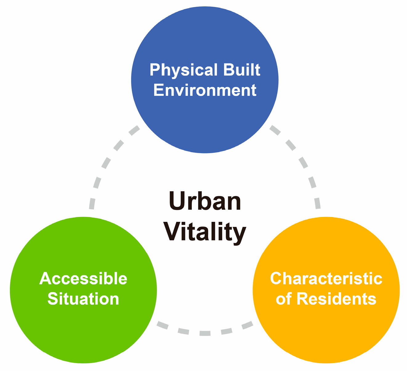
| Factor Type | Indicators | |
|---|---|---|
| Physical built environment | Urban public space | Spatial social interaction coefficient (depends on function) |
| Attractiveness of outdoor landscape and facility | ||
| Building next to the public urban space | Area of ground floor indoor space open to public | |
| Spatial social interaction coefficient (depends on function) | ||
| Openness of buildings | ||
| Negative factors | Trashcan | |
| Homeless | ||
| Others | ||
| Accessible situation | Vehicle accessibility | Reachable by car |
| Distance to parking lot | ||
| Public transport system accessibility | ||
| Walking accessibility | ||
| Access factor, conditions for the urban space entry | ||
| Characteristics of residents | Crowds | Age |
| Occupation and employment status | ||
| Frequency schedule of residents | ||
| Morning | Noon | Night | |
|---|---|---|---|
| Pedestrian Street Entrance | 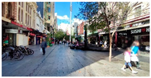 |  |  |
| Pedestrian Street Center |  |  |  |
| Lane Entrance |  |  |  |
| Block Num | Location | Nearby Building Function |
|---|---|---|
| I | Street Side | Bank |
| II | Pedestrian Street Entrance | Retail |
| III | Lane Entrance | Retail |
| IV | Street Side | Apartment and Club |
| V | Street Side | Shopping mall |
| VI | Rest in Lane | Retail |
| VII | Pedestrian Street Node | Retail |
| VIII | Pedestrian Street | Shopping mall |
| IX | Lane Entrance | Shopping mall |
| X | Pedestrian Street Entrance | Retail |
| Frequency of Block II | |||||||
|---|---|---|---|---|---|---|---|
| Days | Weekdays | ||||||
| Crowds | Proportion | 8~10 | 10~12 | 12~14 | 14~16 | 16~18 | 18~20 |
| Retirees | 16% | 0 | 0 | 1 | 1 | 1 | 0 |
| Employed but away from work | 4% | 1 | 1 | 1 | 1 | 1 | 0 |
| Employed full-time | 40% | 0 | 0 | 1 | 0 | 1 | 0 |
| Employed part-time | 27% | 1 | 0 | 1 | 1 | 1 | 0 |
| Unemployed | 7% | 0 | 0 | 1 | 1 | 1 | 1 |
| Teenager students | 4% | 0 | 0 | 1 | 1 | 1 | 0 |
| Young children | 2% | 0 | 0 | 1 | 1 | 1 | 0 |
| Overall | 100% | 0.036 | 0.036 | 0.998 | 0.328 | 0.998 | 0.073 |
| Days | Weekends | ||||||
| Crowds | Proportion | 8~10 | 10~12 | 12~14 | 14~16 | 16~18 | 18~20 |
| Retirees | 16% | 0 | 0 | 1 | 1 | 0 | 0 |
| Employed but away from work | 4% | 1 | 1 | 1 | 1 | 1 | 0 |
| Employed full-time | 40% | 0 | 0 | 1 | 1 | 0 | 0 |
| Employed part-time | 27% | 0 | 0 | 1 | 1 | 0 | 0 |
| Unemployed | 7% | 0 | 0 | 1 | 1 | 1 | 1 |
| Teenager students | 4% | 0 | 1 | 1 | 1 | 1 | 0 |
| Young children | 2% | 0 | 0 | 1 | 1 | 0 | 0 |
| Overall | 100% | 0.036 | 0.074 | 0.998 | 0.998 | 0.147 | 0.007 |
| Regression Statistics Parameters | Multiple R | R2 | p-Value |
|---|---|---|---|
| Result | 0.920637 | 0.847572 | 0.080326 |
| Trusted range | ---- | >0.8 [33,34,35] | <0.1 [36,37] |
| Weekdays Urban Vitality Comparison | Weekends Urban Vitality Comparison | |
|---|---|---|
| Street Side (Block I) |  | 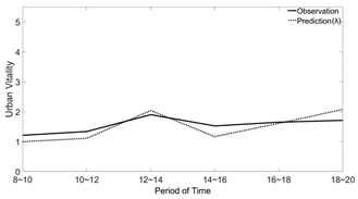 |
| Pedestrian Street (Block II) | 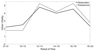 | 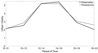 |
| Lane (Block VI) |  |  |
Disclaimer/Publisher’s Note: The statements, opinions and data contained in all publications are solely those of the individual author(s) and contributor(s) and not of MDPI and/or the editor(s). MDPI and/or the editor(s) disclaim responsibility for any injury to people or property resulting from any ideas, methods, instructions or products referred to in the content. |
© 2024 by the authors. Licensee MDPI, Basel, Switzerland. This article is an open access article distributed under the terms and conditions of the Creative Commons Attribution (CC BY) license (https://creativecommons.org/licenses/by/4.0/).
Share and Cite
Liu, Y.; Guo, X. A Dynamic Prediction Framework for Urban Public Space Vitality: From Hypothesis to Algorithm and Verification. Sustainability 2024, 16, 2846. https://doi.org/10.3390/su16072846
Liu Y, Guo X. A Dynamic Prediction Framework for Urban Public Space Vitality: From Hypothesis to Algorithm and Verification. Sustainability. 2024; 16(7):2846. https://doi.org/10.3390/su16072846
Chicago/Turabian StyleLiu, Yue, and Xiangmin Guo. 2024. "A Dynamic Prediction Framework for Urban Public Space Vitality: From Hypothesis to Algorithm and Verification" Sustainability 16, no. 7: 2846. https://doi.org/10.3390/su16072846
APA StyleLiu, Y., & Guo, X. (2024). A Dynamic Prediction Framework for Urban Public Space Vitality: From Hypothesis to Algorithm and Verification. Sustainability, 16(7), 2846. https://doi.org/10.3390/su16072846