Visualizing the Maximum Energy Zone of Wind Turbines Operating at Time-Varying Wind Speeds

Abstract

Wind turbines are one of the leading renewable sources of electricity. They are located in areas where the energy potential of the wind is high and more or less permanent. Their efficient operation depends on certain technical characteristics of the entire wind system (wind turbines, generator, automation system, regulation, and control). This paper analyses experimental data from wind turbines, WT, in the Dobrogea area: wind speed, v, velocity, n, and power, P_EG, at the electric generator, EG. These are used to identify the local maxima of wind turbine power at different wind speeds. Based on this, a mathematical model for wind turbines and the power losses caused by inefficient control are determined. The mathematical model is used to visualize the maximum energy zones. At the end of this study, an algorithm is given that allows for the visualization of the optimal energy zone. The algorithm resulting from the analyzed case studies can be implemented by the control system in order to maximize the produced electricity with any variation in wind speed.

1. Introduction

1.1. Background Information

Wind forecasting techniques are used for the integration of wind turbines into the electricity market and their dispatch. In this way, it is possible to forecast the amount of energy produced, taking into account the dynamics of the electricity market, which are determined by the demand for electricity [1,2], and synchronized with the power curve of the installed wind turbines, which predicts the output as a function of the wind speed [3]. In order to know the wind speed variation curves, it is necessary to make recordings over sufficiently long periods using anemometric towers. In many cases, these data are used in mathematical models to determine monthly wind speed maxima [4]. All these measurements can be used for the individual design of wind turbines, as well as for their selection from a standardized range [5].

Certain methods and control algorithms are chosen depending on the type of turbine and the mode of operation [6,7,8,9]. Adaptive [10] or dynamic control can be used for partial load and rated load operation. This allows for the wind turbine to be controlled even during rapid discharges, when the transient rotor speed tends to increase beyond the limits [11,12,13]. To ensure the more flexible operation of wind farms and turbines, a power monitoring architecture has been proposed through an individual interface with each turbine. The proposed monitoring architecture does not require multiple pieces of information about the turbine dynamics [14]. If a power oscillation damping controller is used, it will affect the wind turbine system to a similar or lesser extent than the wind speed variations [15]. In the case of wind turbines equipped with double-fed induction generators (DFIG), it has been proposed to use a different algorithm to determine the maximum power point using the electrical power values delivered at the output. Based on these values, the wind speed and turbine shaft speed are estimated, allowing for continuous control of the maximum power point operation without the need for a wind speed or turbine shaft speed sensor [16]. There are situations where the simulated peak power point values are higher than those obtained during operation. This can be caused by additional friction that can occur in the cooling system [17].

The value of the optimum mechanical angular velocity, ω_OPTIM, and the power at the electrical generator, P_EG, depend on the value of the wind speed, v, which are generally [18,19,20,21,22] not well known. The maximum capture of wind energy can only be achieved with the correct mechanical angular velocity dependence on the wind speed [18,19,20,23,24]. As atmospheric conditions, mechanical stresses, and even turbine geometry change over time, the dependence of the mechanical angular velocity on the initially set wind speed changes over time and, therefore, requires recalculation based on the measurements [25]. At many sites [22,26,27,28], energy efficiency is reduced due to the age of the turbine’s calibration method, which uses invalid mathematical models.

This study is based on wind speed values, variable speed over time, and visualizing the optimal area from an energy point of view. Most studies have treated existing wind systems based on inadequate calibration methods and without effective wind speed processing. Operating a WT at the point of maximum power, MPP, and at the optimum mechanical angular velocity, MAV, ω_OPTIM, is a complex problem at time-varying wind speeds, due to the high mechanical inertia of wind systems [28,29,30,31,32]. The time variations in wind speed and velocity (mechanical angular velocity), i.e., the functions v(t) and n(t) and ω(t), are continuous and derivable functions. Due to the high mechanical inertia of wind systems [18,33,34], the speed changes slowly over time and it is not a problem to record the current wind speed variations at the site under study [33,35]. The wind speed also changes continuously over time and recording it does not pose any particular problem. Therefore, from measurements, three fundamental quantities are easily and quite accurately known: wind speed, v, power, P_EG, and MAV, ω, at the EG, the basic quantities for WT operation.

Based on these basic quantities, an algorithm is constructed that allows us to visualize the optimal energy zone and to know the dependence of the optimal mechanical angular velocity, ω_OPTIM (v), on the wind speed, v. The dependence of the optimal mechanical angular velocity on the wind speed is the reference quantity in the control design, with which achieves maximum wind energy. For wind power systems operating at v = constant, it is not necessary to know the exact dependence of the optimal MAV, ω_OPTIM, on the wind speed, and the Disturbance and Observe Method, POM, can be applied to the maximum power point, MPP, since it is time-invariant [19,20,23].

In the present study, local speed extremes or the function ω(t) are identified simply by recording the speed over time. Based on the results obtained, the mathematical model of the WT is determined. By visualizing the operating points on the WT power curve, the power losses that occur are estimated. The actual power losses are higher than the calculated ones because the calculations consider some operating points as MPPs, an assumption that cannot be verified due to the lack of more complete experimental data. The visualization of the coordinates of the optimal values is performed during the operation of the wind turbine.

1.2. Specific Objectives and Approach of this Study

The problems addressed in this paper are the mathematical modeling of wind turbines and the calculation of power losses for large variations in wind speed over time, which are fundamental in control design [18,33,34,36,37]. The mathematical model for a wind turbine (WT) is based on the WT power characteristic, the function between the wind speed, v, and the mechanical angular speed, ω, of the turbine, P_WT(ω,v). In most previous papers [18,19,20,23], these issues have been addressed at constant wind speeds over time.

The measurements of wind speed, power, and generator speed were made in Galbiori, Dobrogea [33]. The operating points were positioned on the power characteristic, and compared to the maximum power points, MPPs. Based on the recordings of the fundamental quantities, the MM-WT was determined, a model based on the function P_WT(ω,v), characteristic of the WT power. Mathematical models were calculated for wind speed ranges. The results obtained provide the basis for optimal energy control, with the reference parameters updated in real-time, which is particularly useful for capturing the maximum wind energy, a control that does not exist in the literature. This study highlights the relevant aspects, such as the determination of the turbine power, the operating points where the maximum wind energy is not captured, and the uncertain aspects, where the MPP may be the optimal range of the MAV, ω_OPTIM.

The specialized literature deals just peripherally with the performance of wind turbines operating in areas where the wind potential presents significant variations over time, particularly if those achieve the maximum capture of wind energy. This work aims to estimate the energy efficiency of wind turbines by visualizing the optimal area from the energy point, to locate the operating points of the WT relative to the point of maximum power, corresponding to a certain value of the wind speed. The original contributions of the authors consist in their analysis of the experimental data from 2.5 [MW] wind turbines in operation in the Dobrogea area [33], and determining the extent to which they operate at their maximum power point.

The conducted study is specifically beneficial for assessing the energy efficiency of wind turbines functioning at variable wind speeds over time, as it indicates the area where wind turbines function at the maximum power point.

The main sections of this paper are as follows: an analysis of the wind speed and mechanical speed at the generator; the positioning of the operating points on the WT power curve; the determination of the mathematical model for the WT; the development of an algorithm for determining power losses; discussion, results, and perspectives; and the references used.

2. Wind Speed and Mechanical Speed at the Generator

The analyzed wind turbine at the site in Dobrogea was manufactured by GE (General Electric 2.5 MW series, 100 m rotor diameter), and characterized by an equivalent inertia moment (turbine + gearbox + generator), J = 5372.5 [kgm²], and nominal power obtained at 1500 [rpm]—the nominal rotational speed at the generator level. This study is based on measurements of wind speed, power, and generator speed (=AV) over time, made on 15.06.2022, over a time interval of 280 min, at Galbiori, Dobrogea [18], at a sampling step of 10 [min]. In this area, the variations in wind speed over time are significant. The size of the time interval is important and depends on two important factors: the variation in the wind speed and the value of the equivalent moment of inertia. Considering the variation in the wind speed over time for the analyzed site in the Dobrogea area, and the 2.5 MW installed capacity of the operating wind turbine, we considered that an experimental data set of over 280 min with a 10 min resolution was valid, based on the results obtained through the simulation experiments. At the high value of the equivalent inertia moment, the atmospheric turbulence does not significantly influence the operation of the wind power system. The wind speeds were measured at hub height with a high-precision anemometer. The anemometer could monitor the instantaneous wind speed as well as the wind indicator, measuring the average values for the last two, five, or ten minutes.

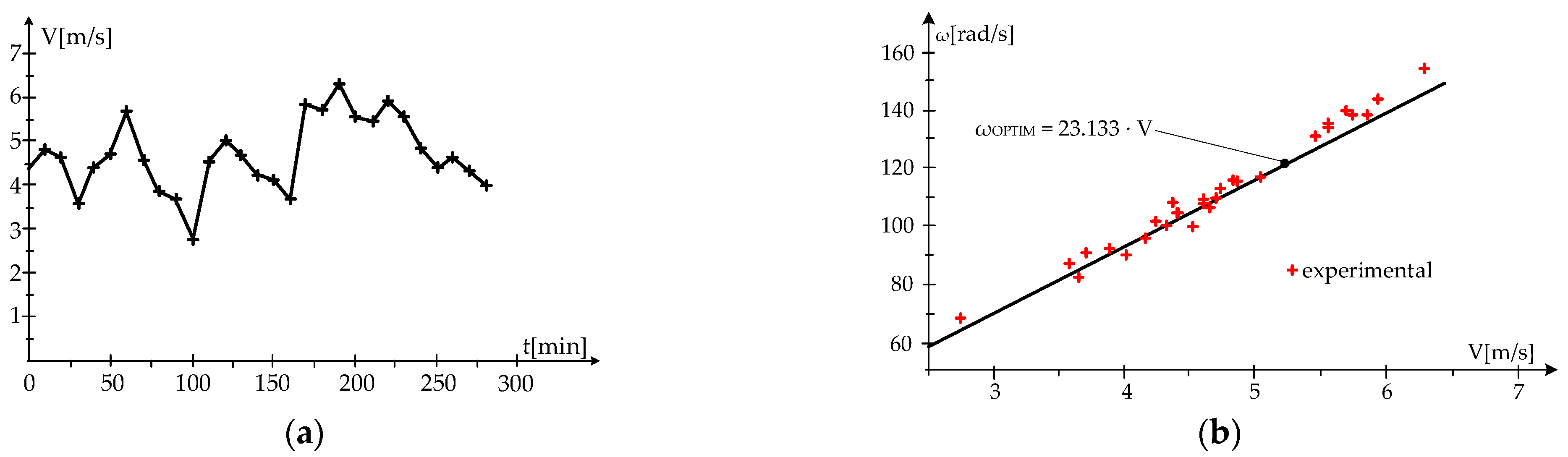
The wind speed changed from 2.7 [m/s] to 6.3 [m/s], and the mechanical angular velocity from 67.963 [rad/s] to 154.41 [rad/s] (Figure 1).

Analyzing the distribution of the wind speed and mechanical angular velocity values given in Figure 1, it follows that:

• In the area with wind speeds greater than 5 [m/s], the measured values of the MAV are larger than those of the ω_OPTIM;
• In the area with wind speeds lower than 5 [m/s], the measured values of the MAV are on either side of the ω_OPTIM, deduced from the mathematical model of the turbine;
• At the maximum wind energy, the measured values of the MAV captured should uniquely define the function ω_OPTIM (v).

The dependence of the optimum mechanical angular velocity of the turbine on the wind speed, the function ω_OPTIM (v), is deduced from the mathematical model of the turbine, MM-WT [23], and has the form:

ω_OPTIM = 23.133 ∙ v

(1)

Based on this, the WT is brought to the MPP and maintained at the optimum MAV, ω_OPTIM, to achieve maximum wind energy capture. In the control design, the use of the MM-WT allows for the optimum mechanical angular velocity, ω_OPTIM, to be determined as a guide, but it must be recalculated periodically as atmospheric conditions, mechanical stresses, and even turbine geometry change over time.

3. Determination of Turbine Power from Generator Power and Speed

The determination of the turbine power, P_WT, is obtained from the kinetic momentum equation [18,21,31,37] with the form:

$$J·\frac{d\omega }{dt} = W_{\mathit{WT}} - W_{\mathit{EG}}$$

(2)

where J is the equivalent moment of inertia; ω is the mechanical angular velocity, MAV, at the electric generator shaft, EG; dω/dt is the time derivative of the MAV; M_WT is the time given by the WT, relative to the EG shaft; and M_EG is the electromagnetic torque given by the EG.

The local maxima and minima are for the rotational speed; the novelty consists in the fact that J, the inertial moment, is no longer needed to compute the WT power because the derivative of the MAV is zero for those local maxima. From the kinetic momentum equation, by multiplying by ω, we obtain the power equation:

$$J·\frac{d\omega }{dt} · \omega = P_{\mathit{WT}} - P_{\mathit{EG}}$$

(3)

where P_WT is the useful power given by the WT, referred to as the shaft of the electric generator, and P_EG is the electromagnetic power of the EG at the shaft.

The power given by the WT, P_WT, is found by the inertial power

$$P_{\mathit{INERTIAL}}=J·\frac{d\omega }{dt} · \omega$$

(4)

and in the power delivered by the electrical generator to the grid, P_EG, according to the equation of motion:

$$P_{\mathit{WT}}=J ·\frac{d\omega }{dt} · \omega + P_{\mathit{EG}}$$

(5)

The power given by the WT is obtained by summing the two powers: the inertial power and the power from the electric generator. The inertial power is determined by recording the rotation MAV at the EG, n/ω, and the power from the electric generator is obtained from the power delivered by the EG to the grid, by dividing by the EG efficiency value.

At the operating points defined by the local extremes of the velocity, the derivative of the mechanical angular velocity, dω/dt, is zero. And because

$$\frac{d\omega }{dt} = 0$$

(6)

the inertial power is zero and the power given by the WT, in the dynamic mode, is equal to the power from the electric generator P_EG:

P_WT = P_EG,

(7)

Therefore, it is not necessary to know the value of the equivalent moment of inertia, J, as the power given by the WT is equal to the power from the EG (which is obtained from the power delivered to the grid by dividing it by the value of the EG output).

Table 1. Measured values of wind speed, v, speed, n, and power, P_EG, at the electric generator.

t [min]	v [cm/s]	n [rpm.]	PEG [kW]
0	437	1033.33	306.22
10	483	1105.52	349.29
20	461	1042.24	278.85
30	358	833.87	152.77
40	441	998.08	242.89
50	471	1043.87	354.09
60	570	1336.66	594.43
70	460	1032.76	280.73
80	389	879.33	163.1
90	370	865.37	145.58
100	274	649.0	35.67
110	452	954.52	259.94
120	504	1115.34	365.84
130	473	1079.00	305.41
140	423	972.12	234.76
150	415	915.46	189.91
160	365	791.02	107.41
170	586	1321.75	628.65
180	574	1318.85	565.51
190	630	1474.47	789.54
200	556	1279.94	532.15
210	546	1249.98	485.47
220	594	1372.09	639.87
230	556	1293.42	535.75
240	486	1101.08	320.12
250	440	999.77	238.16
260	465	1016.9	251.65
270	432	956.25	202.6
280	402	858.33	143.11

shows the measured values of wind speed, velocity, and power delivered by the wind turbine, which change depending on the wind speed. The measurements were taken at 10 min intervals.

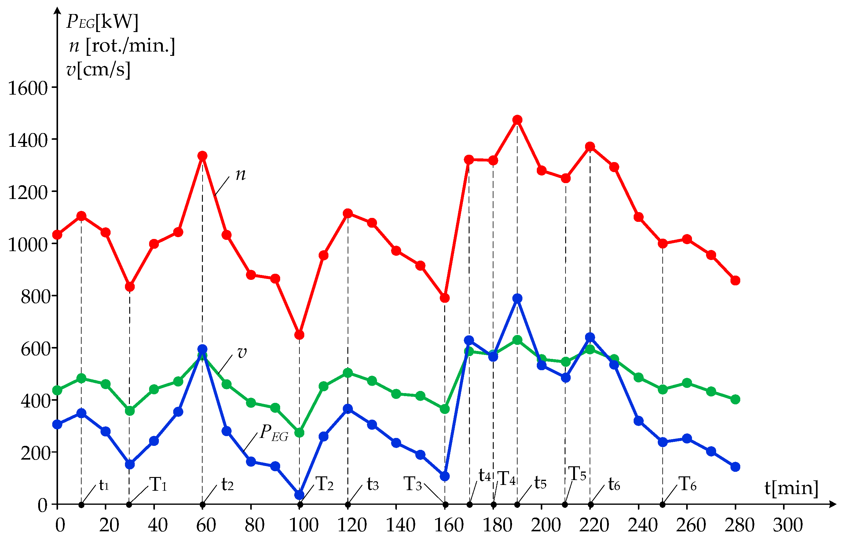
At times t₁, t₂, t₃, t₄, t₅, and t₆, shown in Figure 2, the wind speed, rotation speed, and generator power exhibit the local maxima. Also, at times T₁, T₂, T₃, T₄, T₅, and T₆, they show the local minimum values.

In the following, the measured values of speed and power are compared with the optimal values derived from the mathematical model of the turbine, MM-WT [23], which have the form:

ω_OPTIM = k_n ∙ v

(8)

P_WT-MAX = k_p ∙ v³

(9)

where k_n is the proportionality factor for speed and k_p is the proportionality factor for power.

At these local extremes, the values of wind speed, speed, and power at the generator are the local maxima.

At t₁ = 10 [min], v = 437 [cm/s], n = 1105.52 [rot/min], and P_EG = 306.22 [kW],

n/v = 1105.52/437 = 2.5298

(10)

P_WT = P_EG/v³ = 306.22/437³ = 3.0999 · 10^–6

(11)

Based on (10) and (11), and the values of wind speed, rotational speed, and supplied electric power, we computed the n/v ratio and the P_WT for the 10 min intervals, shown in

Table 2. Values of n/V ratio and P_WT power for maximum wind speed values.

t [min]	n/v	PWT
t1 = 10	2.5298	3.0999 · 10−6
t2 = 60	2.345	3.2098 · 10−6
t3 = 120	2.213	2.8576 · 10−6
t4 = 170	2.2555	3.124 · 10−6
t5 = 190	2.3404	3.1576 · 10−6
t6 = 220	2.3099	3.053 · 10−6

.

Table 3. Measured values of speed and power at local maxima.

v [cm/s]	n [rpm.]	PEG [kW]	Point of Operation
483	1105.52	349.29	A
504	1115.34	365.84	B
570	1336.66	594.43	C
586	1321.75	628.65	D
594	1372.09	639.87	E
630	1474.47	789.54	F

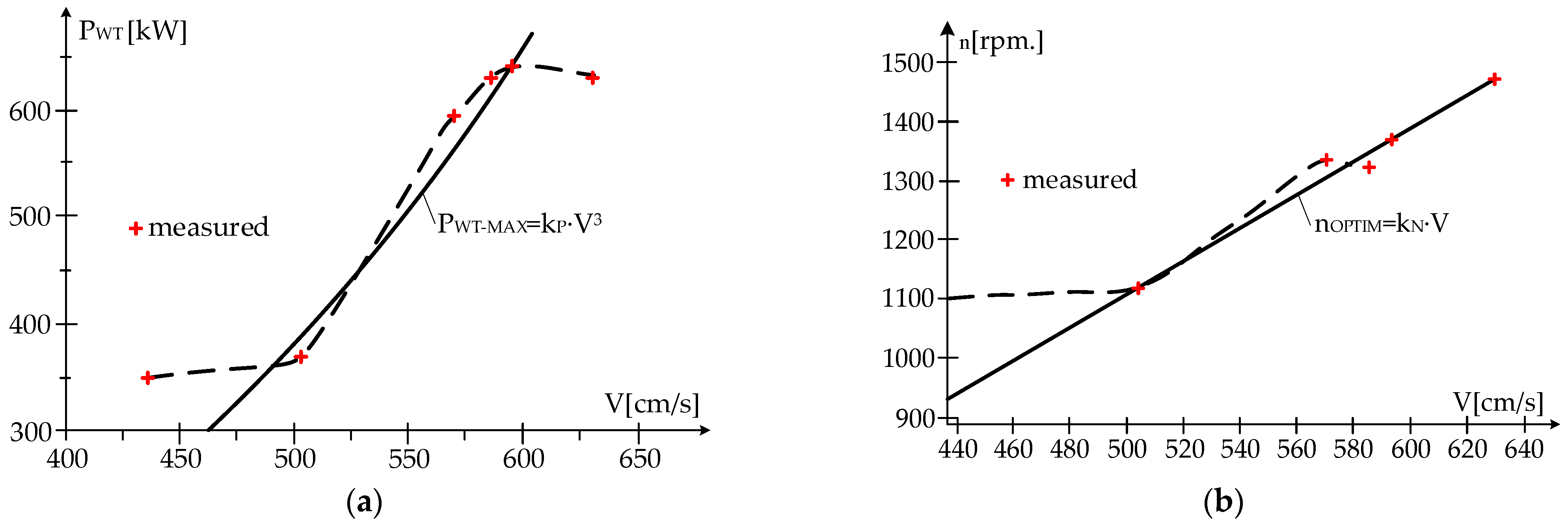
summarizes the values for speed and power at the local maxim (Figure 3).

Figure 4 shows the dependence of power and speed on wind speed at the local maxima, with dash lines representing the interpolation of the measured points.

It can be seen from Figure 4 that for both the power and speed dependencies, the measured values sometimes differ significantly from those given by the functions: n_OPTIM(v) and P_WT–_MAX(v).

The same problems arise for the case of the local minima.

At T₁ = 30 [min], v = 358 [cm/s], n = 833.87 [rot/min], and P_EG = 152.77 [kW],

n/v = 833.87/358 = 2.3292

(12)

P_WT = P_EG/v³ = 152.77/358³ = 3.3296 · 10^–6

(13)

Similarly, we proceeded with the minimum wind speed values and calculated the n/v or P_WT ratio, as shown in

Table 4. n/v ratio and P_WT power for minimum wind speed values.

t [min]	n/v	PWT
T1 = 30	2.3292	3.3296 · 10−6
T2 = 100	2.3686	1.734 · 10−6
T3 = 160	2.1672	2.2088 · 10−6
T4 = 180	2.2976	2.9902 · 10−6
T5 = 210	2.2893	2.9825 · 10−6
T6 = 250	2.2722	2.7958 · 10−6

.

Table 5. Measured values of speed and power at local minima.

v [cm/s]	n [rpm.]	PEG [kW]	Point of Operation
274	649.0	35.67	a
358	833.87	152.77	b
365	791.02	107.41	c
440	999.77	238.16	d
546	1249.98	485.47	e
574	1318.85	565.51	f

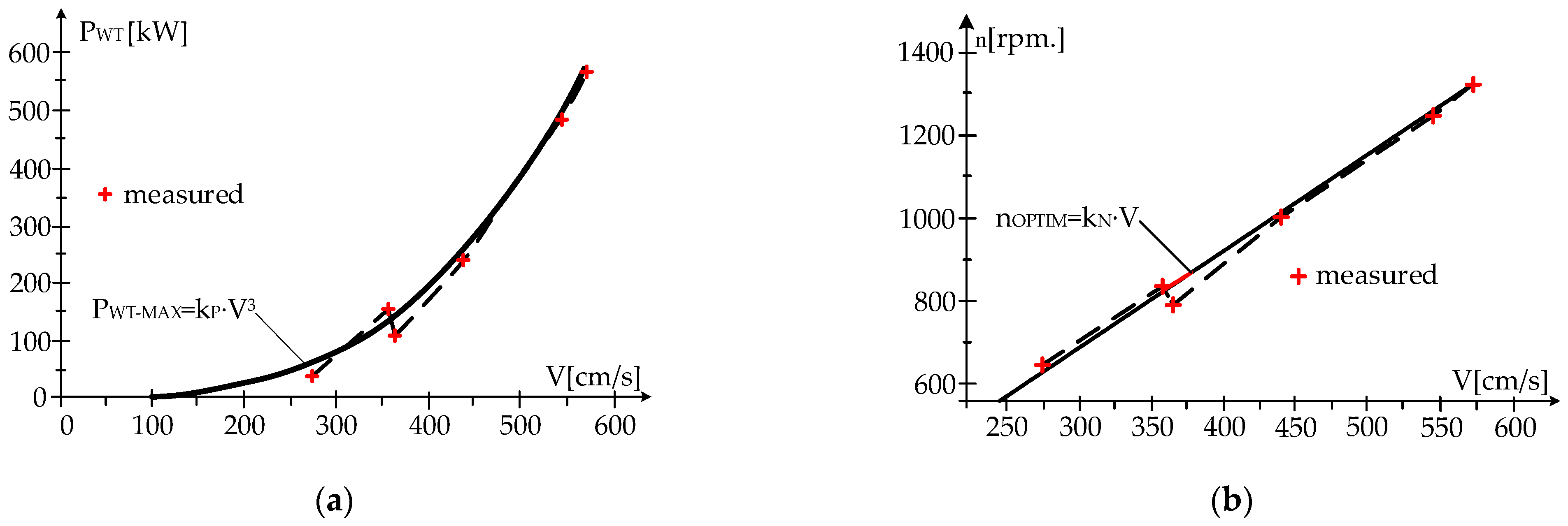
summarizes the values of speed and power at the local minimums.

Figure 5 plots the calculated optimum values against the measured values as well as the interpolation of the measured points, highlighted with dash lines. From the MM-WT, the power and speed dependencies at the local minima are as follows:

n = k_n ∙ v = 2.2976 ∙ v

(14)

P_WT-MAX(v) = k_P · v³ = 3.053 ∙ 10⁻⁶ ∙ v³

(15)

From the MM-WT, the power and speed dependencies at the local minima are

n = k_n ∙ v = 2.2976 ∙ v

(14)

P_WT-MAX(v) = k_P · v³ = 3.053 ∙ 10⁻⁶ ∙ v³

(15)

In this case, too, the measured values are different from those resulting from the functions: n_OPTIM(v) and P_WT-MAX(v). The results obtained are valid only for a sampling step of 10 min, the value for which the design control was built.

4. Positioning of the Operating Points on the Power Characteristic

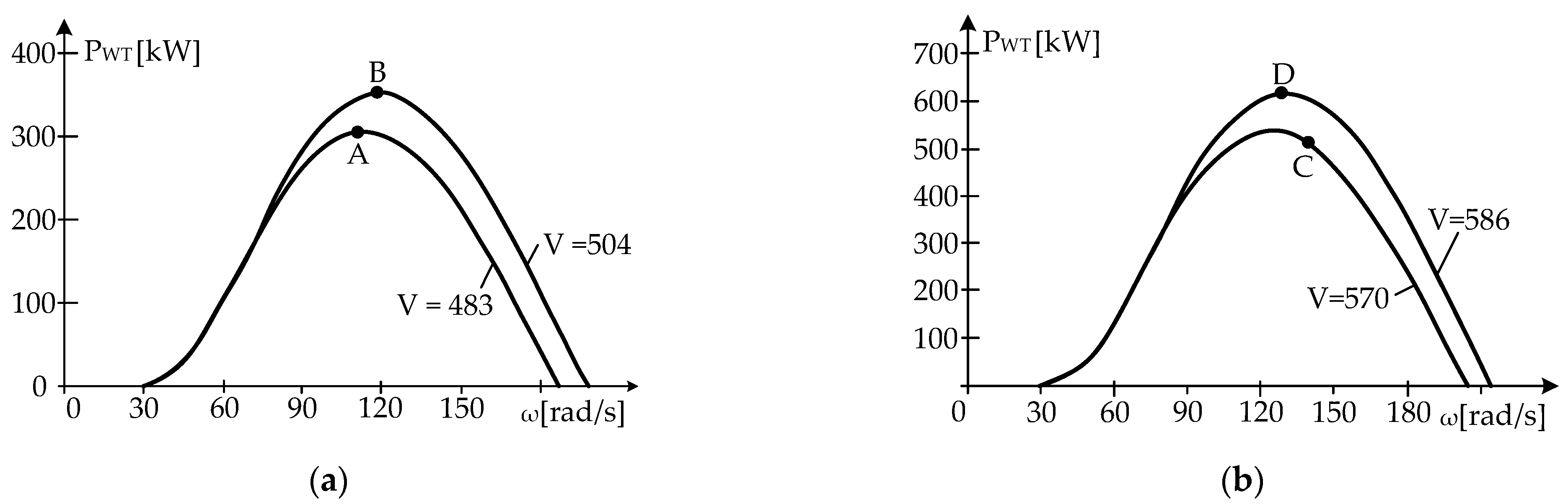
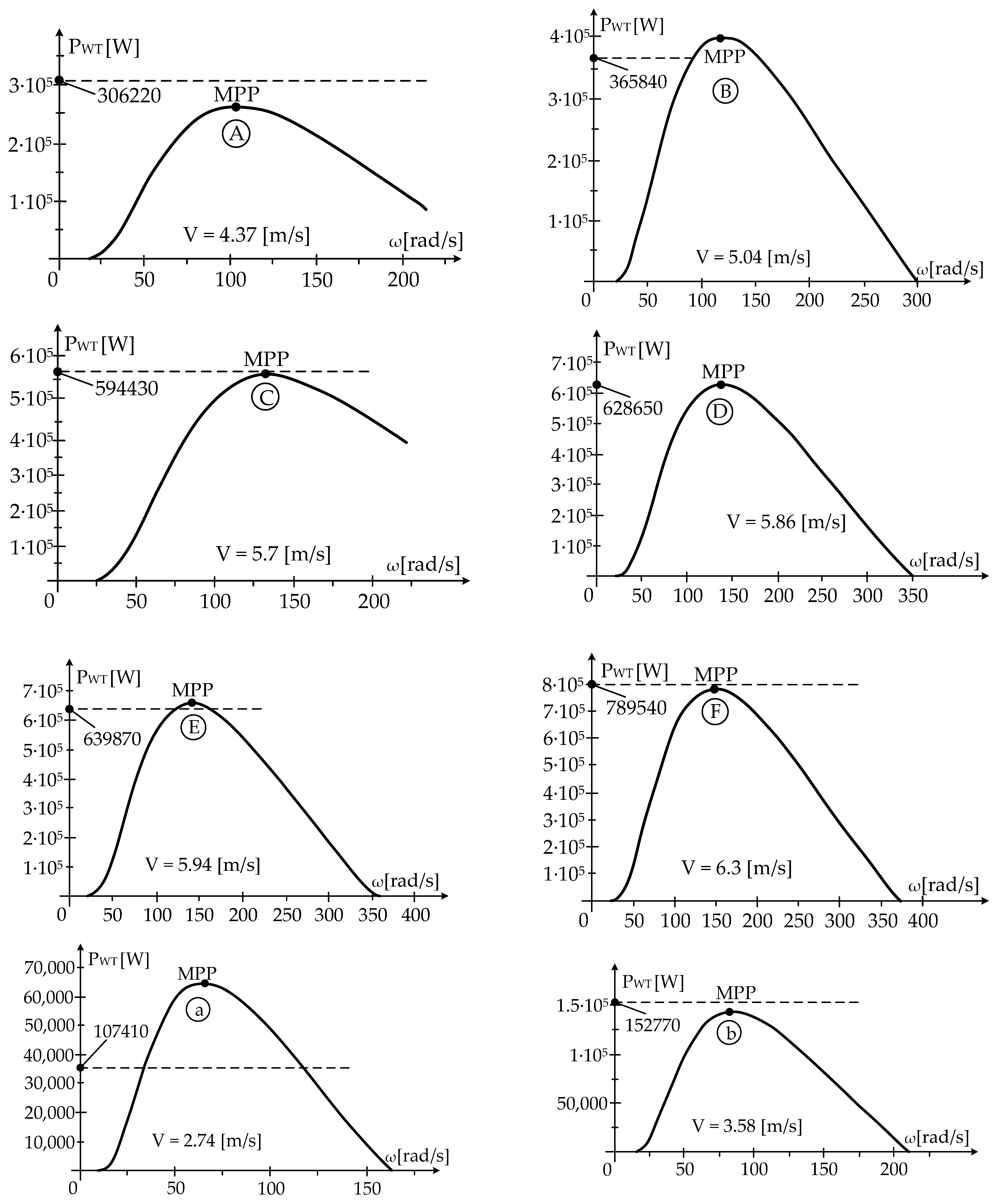
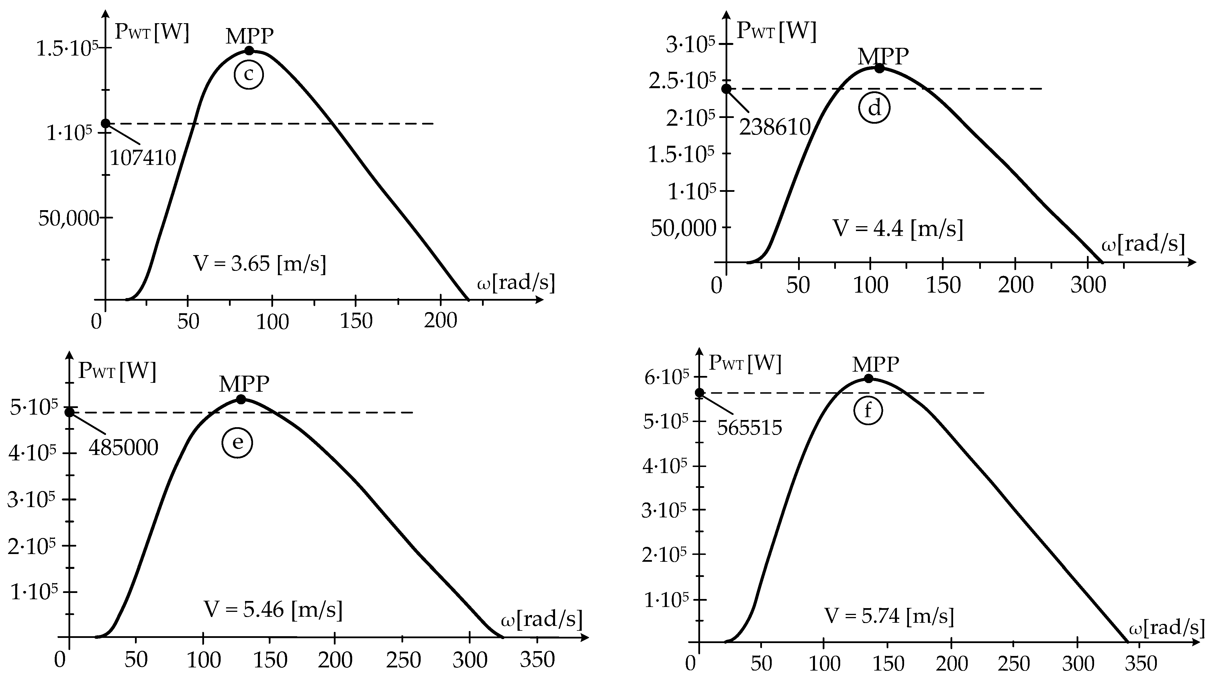
By positioning the operating points on the power characteristic, the P_WT(ω,v) function, the WT operation is visualized in comparison to the maximum power points, MPPs. Given the graph of the power function, P_WT(ω,v), with the maximum, MPP, at ω_OPTIM, the operating points can be approximately located considering the values of the mechanical angular velocity and EG power.

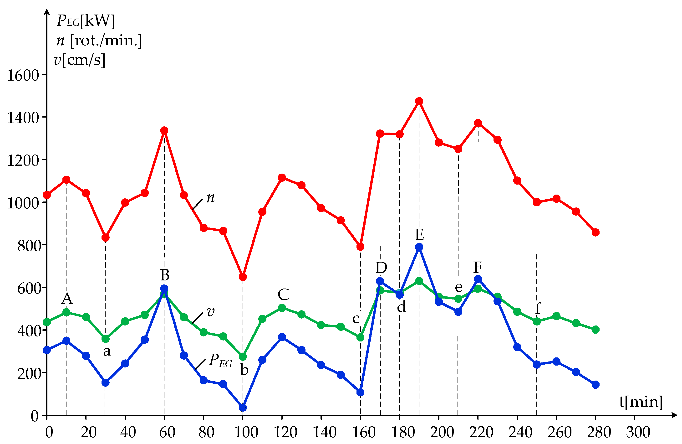
The operating points are A, B, C, D, E, and F at times when the wind speed, speed, and generator power are at the local maxima (Figure 3). At times when v(t), n(t), and P_WT(t) are at the local minima, the operating points are a, b, c, d, e, and f (Figure 3).

In the following, the measured values of speed and power are compared with the optimum values derived from the mathematical model of the turbine, MM-WT [37], which have the form:

n_OPTIM = k_n ∙ v

(16)

P_WT-MAX = k_P · v³

(17)

At these local extreme points, the values of the wind speed, speed, and power at the generator are the operating points A, B, C, D, E, and F at local highs, and a, b, c, d, e, and f, at local lows, which are, probably, in the MPP area (Figure 3).

The location of the operating points is approximate because the coordinates of the maximum power point (MPP) are not known with certainty and will change over time for wind systems operating at wind speeds that vary significantly over time. At the local maxima for the function n_OPTIM(v), the operating points can be seen in Figure 6.

P_WT(ω, 4.09) = 1453 ∙ 10⁴ (4.09/ω − 2.6345 · 10⁻²) ∙ e^{−58.398(4.09/ω)} ∙ 4.09³

(18)

P_WT(ω, 4.2828) = 1453 ∙ 10⁴ (4.2828/ω − 2.6345 · 10⁻²) ∙ e^{−58.398(4.2828/ω)} ∙ 4.2828³

(19)

Operating point A:

ω_A = π ∙(1105.52/30) = 115.77 [rad./s.] P_WT-A = 349.29 [kW]

(20)

For the other operating points, we proceeded in a similar way and the results are shown in

Table 6. Values for ω and P_WT for operating points at local maxima.

Point of Operation	ωA [rad./s.]	PWT-A [kW]
A	115.77	349.29
B	116.8	365.84
C	139.97	594.43
D	134.81	628.65

.

The operating points E and F are not represented because they are not of interest, probably being the MPPs, since their speeds and powers may be the optimal values, n_OPTIM and P_WT–MAX.

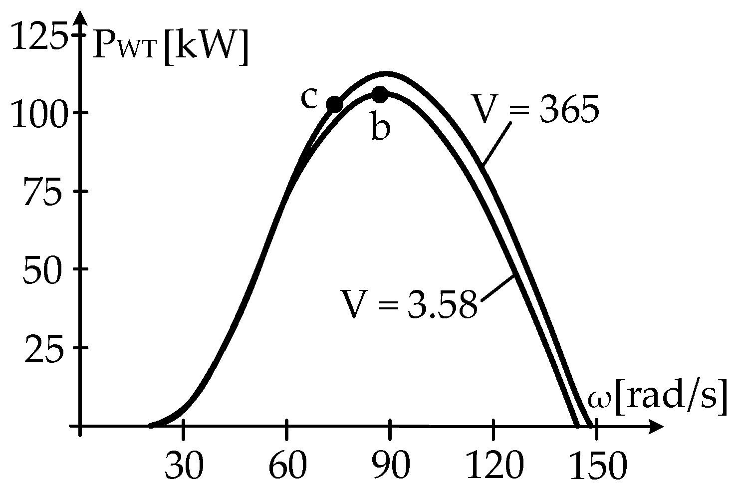
V_c is 365 for point c and v_b is 358 for point b. At the local minima, the operating points of interest are b and c, shown in Figure 7, because at c the rotational speed is lower than at b, though at c the wind speed is higher than that at b:

v_c = 365 [cm/s] > v_b = 358 [cm/s]

(21)

ω_b = π ∙(833.87/30) = 87.32 [rad./s.] for point of function b

(22)

ω_c = π ∙(791.02/30) = 82.835 [rad./s.] for point of function c

(23)

The positioning of the operating points was performed based on the coordinates of these points: ω (MAV) and power at the EG. The following conclusions can be drawn from the positioning of the operating points:

• Points B, D, E, F, and b can be MPPs, but this cannot be stated with certainty, as the exact coordinates of the points, ω_OPTIM and P_WT-MAX, are not known;
• Points A, C, and c cannot be MPPs, because their speeds are above the optimum values, n_OPTIM;
• The dependence of the optimal wind turbine speed on the wind speed is not a linear function, n_OPTIM = kV; as a result of the MM-WT, it depends on many factors;
• The MPP coordinates, ω_OPTIM and P_WT–MAX, can only be determined by running the WT in the area ∆ω = (0.9–1.1) · ω_OPTIM, passing through the MPP.

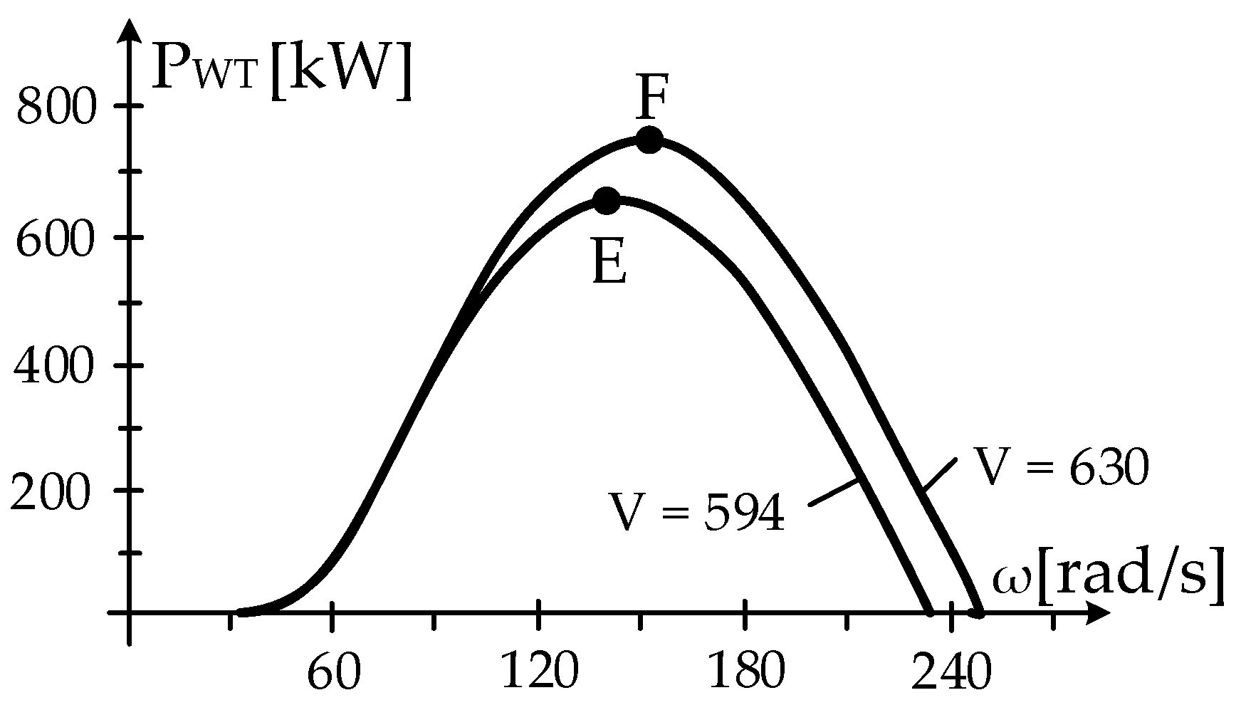
The operating points E and F can be MPPs because their coordinates are

Point of operation E:

ω_E = π ∙(1336.66/30) = 139.97 [rad/s] P_WT-E = 594.43 [kW]

(24)

Point of operation F:

ω_F = π ∙(1474.47/30) = 154.41 [rad/s] P_WT-F = 789.54 [kW]

(25)

which are probably equal to the optimum, as illustrated in Figure 8.

Further, with regard to the WT power characteristic, the function P_WT(ω) changes significantly with time and at varying wind speeds, and for high values of the equivalent moment of inertia J, it is difficult to determine the MPP coordinates. The results obtained are useful in determining the mathematical model for the WT.

5. Mathematical Model of the Turbine

Based on the time records of the fundamental parameters of wind speed, v, and rotational speed and power at the EG, the MM-WT can be determined; a model that is particularly important both for the optimal control of wind power plants and for the estimation of their performance under high temporal wind speed variations. The mathematical model for a WT at wind speed v is embodied in the WT power characteristic function, P_WT(ω,v).

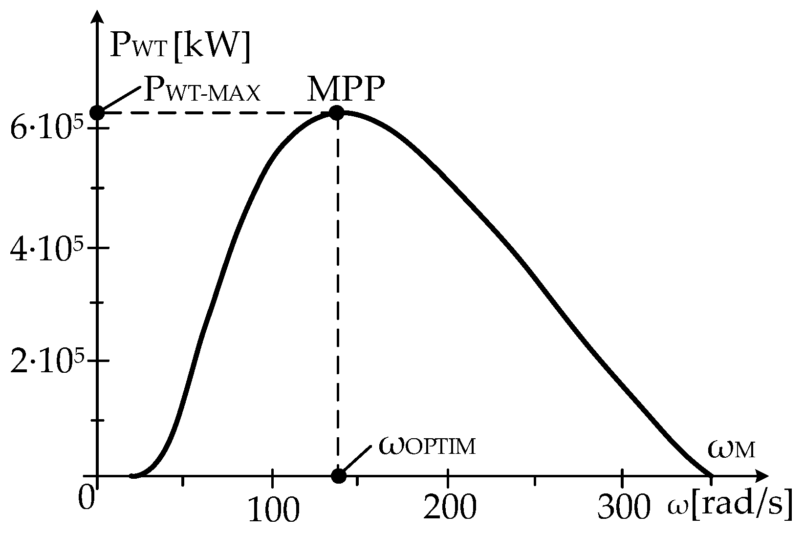
The maximum of the P_WT(ω,v) function is at the point of maximum power, MPP (Figure 9), whose coordinate points are given by the optimum mechanical angular velocity, ω_OPTIM, and the maximum power, P_WT–MAX.

In the idle operation of the WT, the mechanical angular velocity has the maximum value, ω_M. In the control design, the MPP area and knowledge of the dependence of the optimal mechanical angular velocity, ω_OPTIM, on the wind speed are essential. This fundamental problem is addressed in this paper.

This MM-WT can be updated in real-time to ensure maximum wind energy capture. The mathematical model of the wind turbine determines the optimum speed as a function of the wind speed. Various forms of the WT power curve, the P_WT(ω,v) function, have been given in the literature [18,19,20,21,22,23,31].

The most useful case is that with three parameters– a, b, and c—with the form:

P_WT(ω,v) = a[(v/ω) − b] · e^−c(v/ω) ·v³

(26)

Parameters a, b, and c are determined by measuring the following: the wind speed, v, the power flow, P_EG, and the rotation speed/mechanical angular velocity at EG, n/ω.

The coordinates of the maximum power points, MPPs, are obtained from

dP_WT/dω = 0

(27)

or

d {[(v/ω) − b/]·e^−c(V/ω)}/dω = −(v/ω³) · e^−V·(c/ω) · (ω − v · c + b · c · ω) = 0

(28)

with the solution

ω_OPTIM = v · c/[ (b · c) + 1]

(29)

and maximum power:

P_WT-MAX = a · {(1/c) · [(b · c) + 1] − b} · e^{−c·{(1/c) · [(b · c)+1]}} ·v³ = v³ · (a/c) · e^−bc−1

(30)

The maximum value of VUM, ω_M, is at P_WT = 0, resulting in

(v/ω_M) − b = 0, and ω_M = v/b

(31)

It is known from the literature [18,19,20,23,36,37] that the value of the ratio ω_OPTIM/ω_M is

(ω_OPTIM/ω_M) = {(v · c)/[(b · c) + 1]}/(v/b) = (b · c)/[(b · c) + 1] = 0.4

(32)

which gives the value of the product b · c:

b · c = 0.66667

(33)

With this value we obtain

P_WT-MAX = v³ · (a/c) · e^−bc−1 = 0.18887 · (a/c) · v³

(34)

At operating points B, D, E, F, and b, which can be MPPs, the values of the ratios a/c = x are

Point of function C, 365.84 = 0.18887 · x · 5.04³ with solution 15.13

(35)

Point of function D, 628.65 = 0.18887 · x · 5.86³ with solution 16.541

(36)

Point of function E, 789.54 = 0.18887 · x · 6.3³ with solution 13.34

(37)

Point of function F, 639.87 = 0.18887 · x · 5.94³ with solution 16.165

(38)

Point of function a, 152.77 = 0.18887 · x · 3.58³ with solution 17.629

(39)

When operating in an MPP, the values of the a/c reports should be the same, but, if they are not equal at those points, the captured wind energy is not at a maximum and, hence, some operating points are not MPPs.

5.1. First Case Study

For the determination of the MM-WT, the operating point D is chosen as the MPP, although this cannot be stated with certainty, as the coordinates of this point are not known exactly.

At operating point D, the wind speed, speed, and power have values of v = 586 [cm/s], n = 1321.75 [rot/min], and P_EG = 628.65 [kW], from which it follows that

ω_D = (π/30) · 1321.75 = 138.41 [rad/s]

(40)

P_WT/v³ = 628,650/5.86³ = 0.18887 · (a/c)

(41)

and we obtain

a/c = 16,540, or a = 16,540 · c

(42)

With this data, the WT power characteristic, the function P_WT (ω, v), becomes

P_WT(ω, 5.86) = a · [(v/ω) − b] · e^−c(v/ω) · v³

(43)

P_WT(ω, 5.86) = 16,540 · c [(5.86/138.41) − b] · e^{−c(5.86/138.41)} · 5.86³

(44)

62,850 = 16,540 · (4.2338 · 10⁻² · c −0.66667) · e^{−c(5.86/138.41)} · 5.86³

(45)

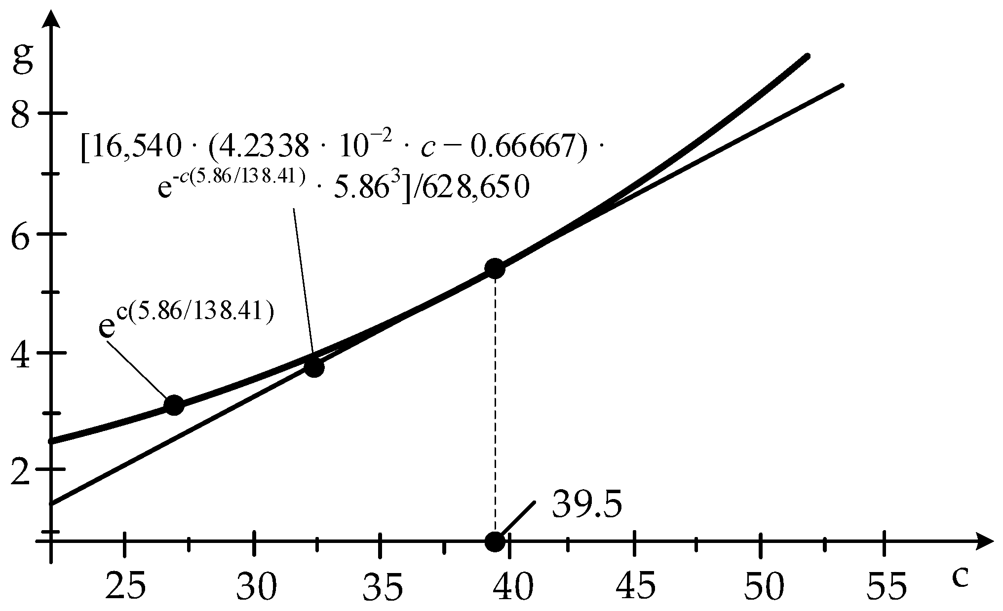
From this equation, the parameter c is determined as follows:

e^{c(5.86/138.41)} = [16,540 · (4.2338 · 10⁻² · c − 0.66667) · 5.86³]/628,650

(46)

The value of parameter c is obtained from the intersection of the two graphs (Figure 10) and is c = 39.5.

From bc follows the value of parameter b:

b = bc/c = 0.66667/39.5 = 1.6878 · 10⁻²

(47)

When a/c = 16,540, this results in a value of parameter a of

a = 16,540 · c = 16,540 · 39.5 = 6.5333 · 10⁵

(48)

and, thus, the WT power characteristic, the function P_WT(ω, 5.86), or the MM-WT, is obtained in the form:

P_WT(ω, 5.86) = a[(v/ω) − b]· e^−c(v/ω) · v³

(49)

P_WT(ω, 5.86) = 6.5333·10⁵ (5.86/ω − 1.6878·10⁻²) · e^{−39.5(5.86/ω)} · 5.86³

(50)

The mathematical model of a WT at wind speed v is expressed as follows:

P_WT(ω, v) = 6.5333·10⁵(v/ω − 1.6878·10⁻²) · e^{−39.5(v/ω)} · v³

(51)

Figure 11 shows the WT power characteristics, the function P_WT (ω, v).

From the analysis of the WT power characteristics given above, it appears that there are large differences between the measured and the corresponding MPPs, P_WT–MAX.

At operating points A, C, and b, a paradoxical situation occurs: the power given by the WT is higher than the maximum value, P_WT–MAX, which invalidates the MM-WT deduced from the data at operating point D. It seems that the MM-WT cannot be applied over the whole range of wind speeds, because in the low-speed range

v = (2.74 … 3.65) [m/s]

(52)

and large differences occur between the measured powers and the corresponding MPPs, compared to the area of higher speeds

v = (5.4 … 6.3) [m/s]

(53)

where the differences in power are smaller.

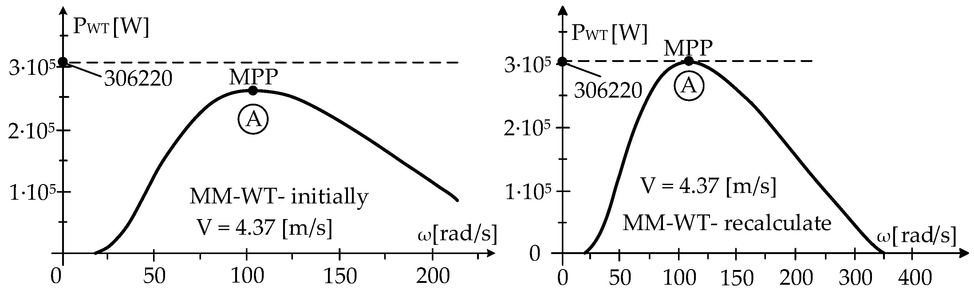
To eliminate this paradoxical situation at operating point A, the MM-WT is recalculated.

5.2. Recalculation of MM-WT

The MM-WT recalculation is performed with data from operating point—A—MM-WT-recalculated-1.

At operating point A, the wind speed, speed, and power have values of v = 437 [cm/s], n = 1033.33 [rot/min], and P_EG = 306,220 [W], from which it follows that

ω_A = (π/30) · 1033.33 = 115.77 [rad/s]

(54)

P_WT/v³ = 306,220/4.37³ = 3669.4 = 0.18887 · (a/c)

(55)

and we obtain

a/c = 9428, or a = 19,428 · c

(56)

With this data, the WT power characteristic, the function P_WT (ω, v), becomes

P_WT(ω, 4.37) = a[(v/ω) − b] · e^−c(v/ω) · v³

(57)

P_WT(ω, 4.37) = 19,428 · c (4.37/108.21 − b) · e^{−c(4.37/108.21)} · 4.37³

(58)

306,220 = 19,428 · (4.0384 · 10⁻² · c − 0.66667) · e^{−c(4.0384 · 10−2)} · 4.37³

(59)

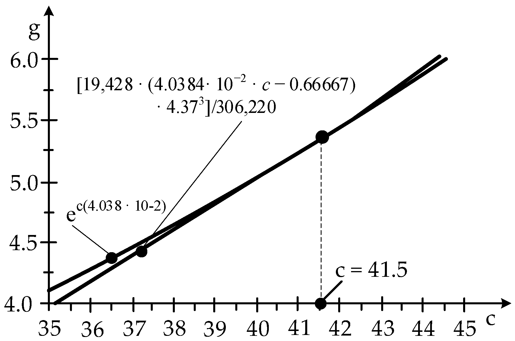
From this equation, the parameter c is determined as follows:

e^{c(4.0384 · 10−2)} = [19,428 · (4.0384· 10⁻² · c − 0.66667) · 4.37³]/306,220

(60)

The value of parameter c is obtained from the intersection of the two graphs (Figure 12) and is c = 41.5.

From bc results the value of parameter b:

b = bc/c = 0.66667/41.5 = 1.6064 · 10⁻²

(61)

When a/c = 19,428, this results in a value of parameter a of

a = 19,428 · c = 19,428 · 41.5 = 8.0626 · 10⁵

(62)

and, thus, the WT power characteristic, the function P_WT(ω, 4.37), or the MM-WT-recalculated-1, has the form:

P_WT(ω, 4.37) = a[(v/ω) − b]· e^−c(v/ω) · v³

(63)

P_WT(ω, 4.37) = 8.0626 · 10⁵ (4.37/ω − 1.6064·10⁻²) · e^{−41.5(4.37/ω)} · 4.37³

(64)

With this form of the MM-WT, operating point—A becomes the MPP, as shown in Figure 13.

This form of the MM-WT, derived from the data from operating point A, is closer to reality, but it cannot be said with certainty that operating point A is the MPP. It can, however, be stated with certainty that the operating points B, D, a, c, d, e, and f in Figure 11 are not the MPP. Other points could be chosen, apart from operating point A, for the MM-WT deduction, but these points, however, must have a measured power value, P_WT-MES, greater than or equal to the maximum, P_WT–MAX:

P_WT-MES > P_WT-MAX

(65)

The mathematical model of the WT, recalculated at wind speed v, is as follows:

P_WT(ω,v) = 5.97144 · 10⁵(v/ω − 1.6064 · 10⁻²)e^{−41.5(v/ω)} · v³

(66)

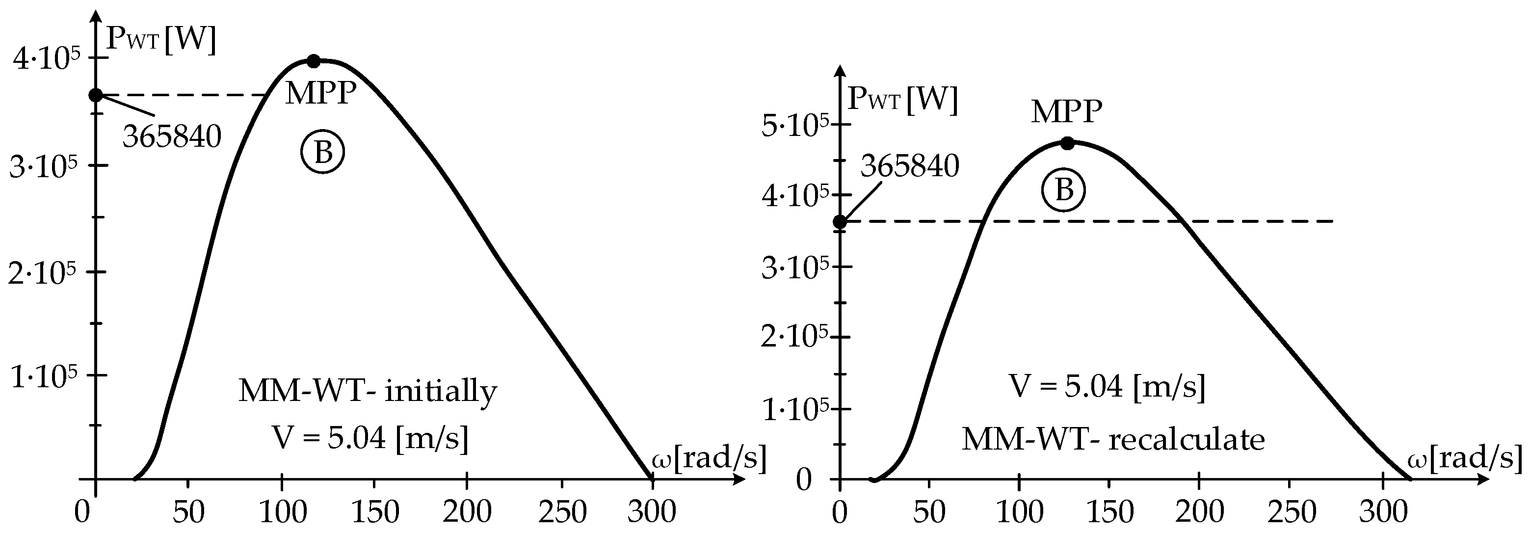
5.3. Comparison of the Two MM-WTs

Comparing these two MM-WTs, it can be seen from Figure 14 that the calculated MM-WT operating point B is further away from the MPP than that in the original MM-WT.

Not only by comparing the WT power characteristics graphs, shown in Figure 14, can one assert this, but also by calculations based on the previous results:

• With MM-WT-initial:

P_WT-MAX = 0.18887 · 16,540 · v³ = 3123.91 · v³

(67)

• With MM-WT-recalculated-1:

P_WT-MAX = 0.18887 · 19,428 · v³ = 3669.4 · v³

(68)

At operating point B, the wind speed has a value v = 5.04 [m/s], and we obtain the following:

• With MM-WT-initial:

P_{WT-MAX-INITIAL} = 3123.9 · 5.04³ = 3.9993 · 10⁵ [W]

(69)

• With MM-WT-recalculated-1:

P_{WT-MAX-RECALCULATED-1} = 3669.4 · 5.04³ = 4.6977 · 10⁵ [W]

(70)

The power differences between the maximum values, calculated as the follow-ups P_{WT–MAX–INITIAL} and P_{WT–MAX–RECALCULATED–1}, and the measured value at operating point B, P_WT-MES-B = 365,840 [W], are as follows:

• With MM-WT-initial:

ΔP_WT-INITIAL = P_{WT-MAX-INITIAL} − P_WT-MES-B = 3.9993 · 10⁵ − 365,840 = 34,090 [W]

(71)

• With MM-TV-recalculated-1:

ΔP_{WT-RECALCULATED} = P_{WT-MAX-RECALCULATED} − P_WT-MAS-B = 4.6977·10⁵ − 365,840

(72)

ΔP_{WT-RECALCULATED} = 1.0393 · 10⁵ [W]

(73)

So, this calculation also confirms that B is not an operating point in the MPP. The power loss at operating point B is large:

ΔP = (ΔP_{WT-RECALCULATED}/P_{WT-MAX-RECALCULATED-1}) ·100

(74)

ΔP = (1.0393 · 10⁵/4.6977 · 10⁵) · 100 = 22.124%

(75)

This form of the MM-WT, deduced based on data from operating point A, is closer to reality, but it cannot be stated with certainty that operating point A is the MPP. It can be stated with certainty that operating points C, D, a, c, d, e, and f in Figure 11 are not the MPP. A, for the MM-WT deduction, has points which, however, must have a measured power value, P_WT-MES, greater than or equal to the maximum, P_WT–MAX:

P_WT-MES ≥ P_WT-MAX

(76)

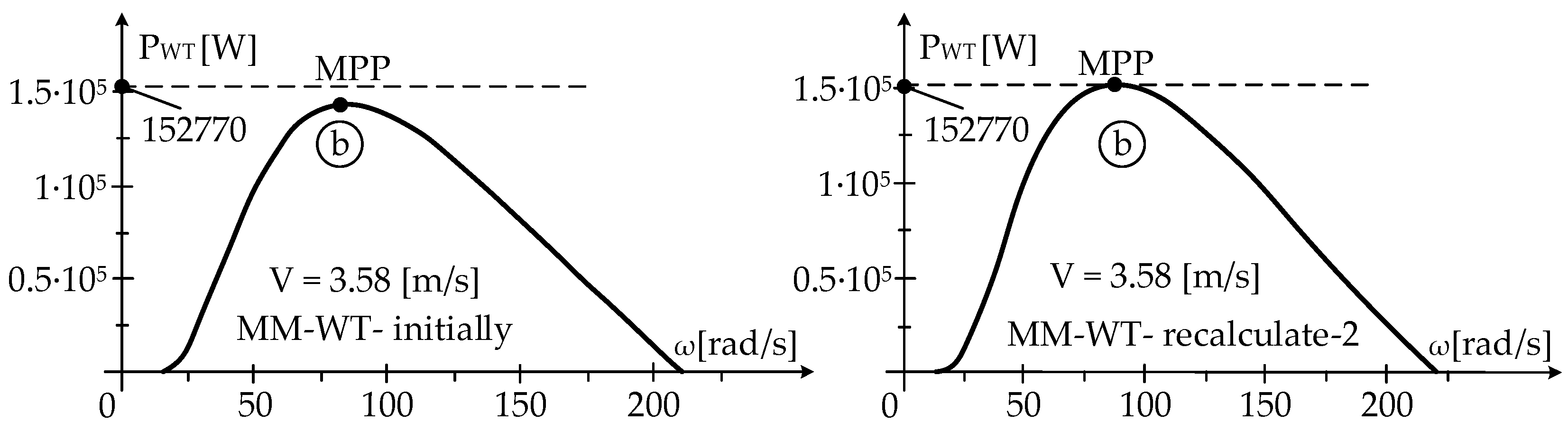
5.4. The MM-WT Recalculation in the Low-Speed Zone

In the range of low wind speeds, 3 [m/s], where the differences between the performances are large, a recalculation of the MM-WT is also required. The MM-WT recalculation is performed with data from operating point b MM-WT-recalculated-2. At operating point b, the wind speed, speed, and power have values of v = 3.58 [m/s], n = 833.87 [rot/min], and P_EG = 152,770 [W], from which it follows that

ω_b = (π/30) · 833.87 = 87.323 [rad/s]

(77)

P_WT/v³ = 152,770/3.58³ = 33,296 = 18,887 · (a/c)

(78)

and we obtain

a/c = 17,629, or a = 17,629 · c

(79)

The WT power feature becomes

P_WT(ω, 4.37) = a[(v/ω) − b] · e^−c(v/ω) · v³

(80)

P_WT(ω, 4.37) = 17,629 · c (3.58/87.323 − b) · e^{−c(3.58/87.32321)} · 3.58³

(81)

152,770 = 17,629 · (4.0997 · 10⁻² · c − 0.66667) · e^{−c(3.58/87.32321)} · 3.58³

(82)

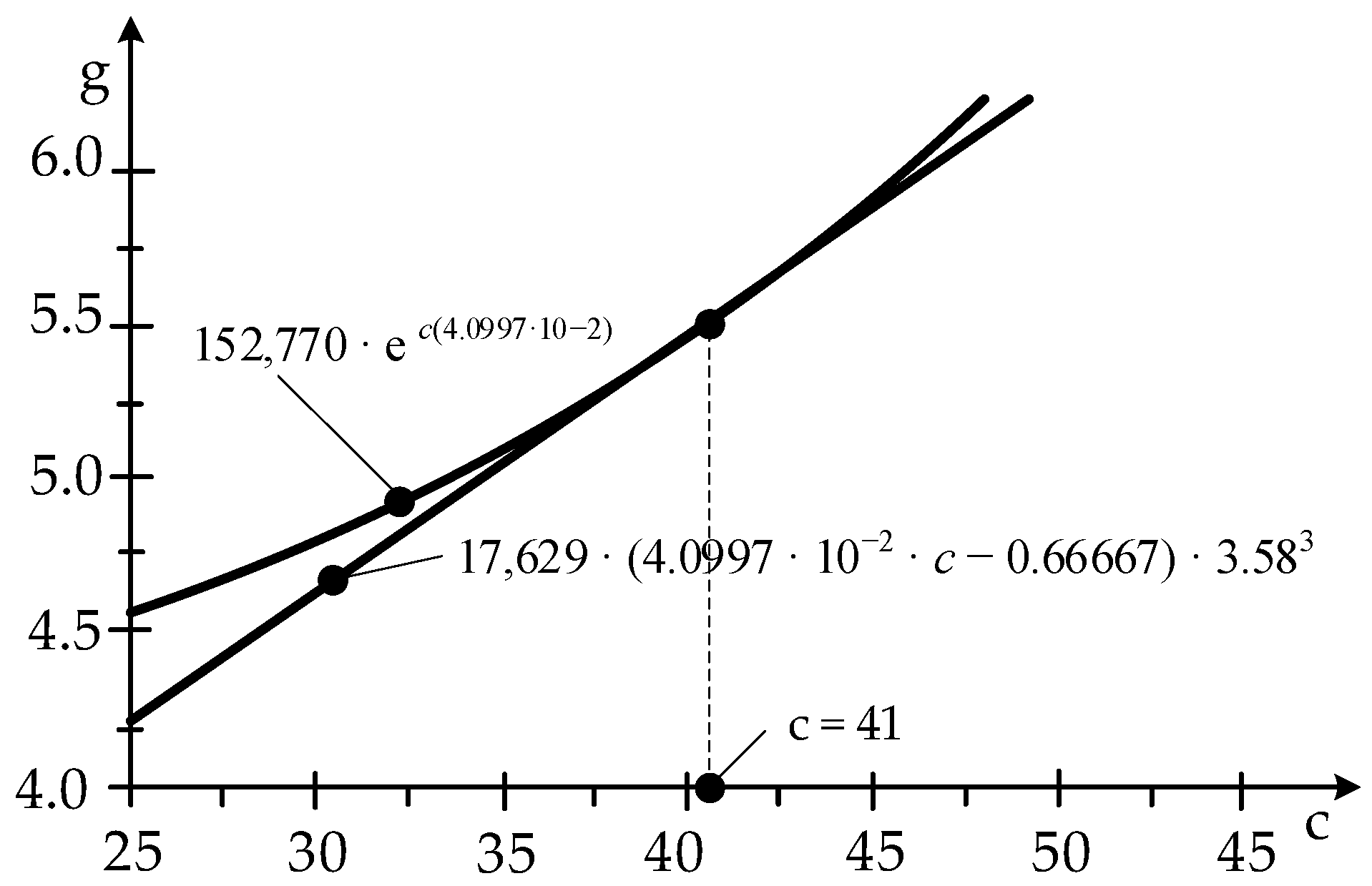
From this equation, the parameter c is determined by

152,770 · e ^{c(4.0997·10−2)} = 17,629 · (4.0997 · 10⁻² · c − 0.66667) · 3.58³

(83)

according to the two graphs in Figure 15, resulting in c = 41.

From b · c results the value of parameter b:

b = bc/c = 0.66667/41 = 0.01626

(84)

When a/c = 17,629, this results in a value of parameter a of

a = 17,629 · c = 17,629 · 41 = 7.2279 · 10⁵

(85)

and, thus, the WT power characteristic, the function P_WT (ω, 3.58), or the MM-WT-recalculated-2, has the form:

P_WT(ω, 3.58) = a[(v/ω) − b]· e^−c(v/ω) · v³

(86)

P_WT(ω, 3.58) = 7.2279 · 10⁵ (3.58/ω − 0.01626) · e^{−41(3.58/ω)} · 3.58³

(87)

The mathematical model of the WT at wind speed v is expressed as follows:

P_WT(ω, v) = 7.2279 · 10⁵ (v/ω − 0.01626) · e^−41(v/ω) · v³

(88)

Operating point b, with this form of the MM-WT, becomes the MPP (Figure 16).

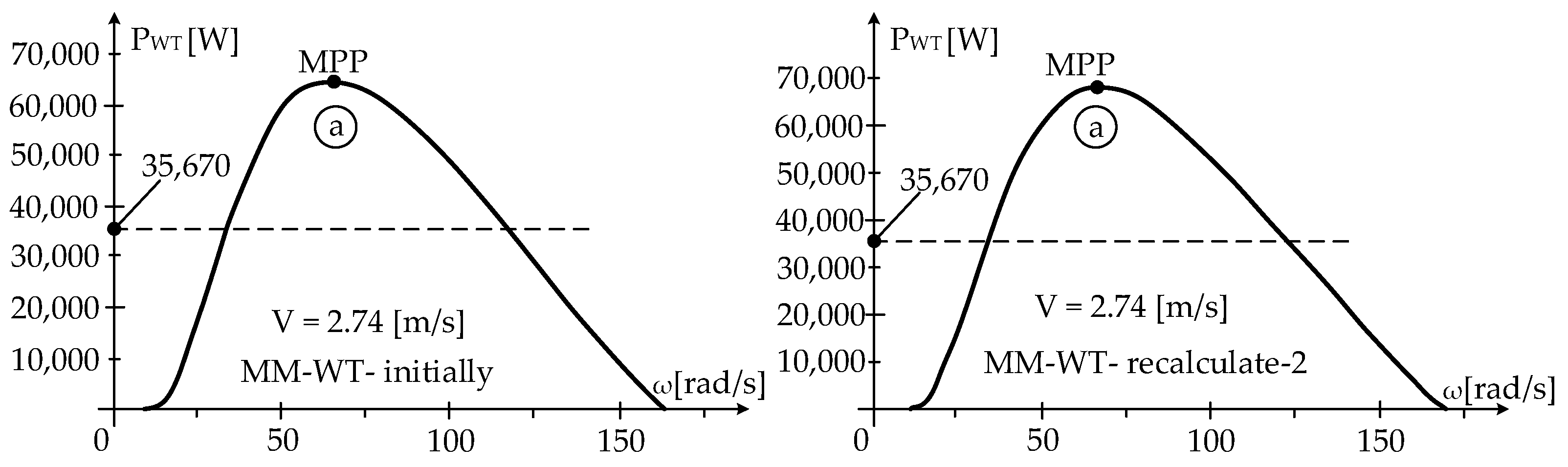
Further analyzing operating point-a, it can be seen from Figure 17 that the power difference between the measured value, P_WT-MES-a, and the maximum value, P_WT–MAX, is increased in the MM-WT-recalculated-2 version compared to the MM-WT-initial. At operating point-a-, the wind speed has a value v = 2.74 [m/s]. Operating point a is further away from the MPP in the MM-WT-recalculated-2 version.

This can also be stated by calculations, as follows:

• With MM-WT-initial:

P_{WT-MAX-INITIAL} = 0.18887 · 16,540 · v³ = 3123.9 · v³ = 3123.9 · 2.74³ = 64,261 [W]

(89)

• With MM-WT-recalculated-2:

P_{WT-MAX-RECALCULATED-2} = 0.18887·17,629 · v³ = 3329.6 · v³ = 3329.6 · 2.74³ = 68,493 [W]

(90)

The power differences between the maximum values, P_{WT–MAX– INITIAL} and P_{WT–MAX– RECALCULATED–2}, and the measured value at operating point a are P_WT-MES-a = 35,670 [W]. This can also be expressed as follows:

• With MM-WT-initial:

ΔP_WT-INITIAL = P_{WT-MAX-INITIAL} − P_WT-MES-a = 64,261 − 35,670 = 28,521 [W]

(91)

• With MM-WT-recalculated:

ΔP_{WT-RECALCULATED} = P_{WT-MAX-RECALCULATED-2} − P_WT-MES-a = 68,493 − 35,670 = 32,823 [W]

(92)

It is confirmed that operating point a not is the MPP. The power loss, ∆P, at operating point a is very high:

ΔP = (ΔP_{WT-RECALCULATED}/P_{WT-MAX-RECALCULATED-2}) · 100

(93)

ΔP = (32,823/68,493) ·100 ≈ 48%

(94)

In reality, at the point of operation, the power loss is higher and can exceed 50%, so only half of the wind energy is captured that could be captured at MPP operation, at a_OPTIM. With this data, an algorithm can be constructed to determine the power losses occurring in wind power systems operating at time-varying wind speeds.

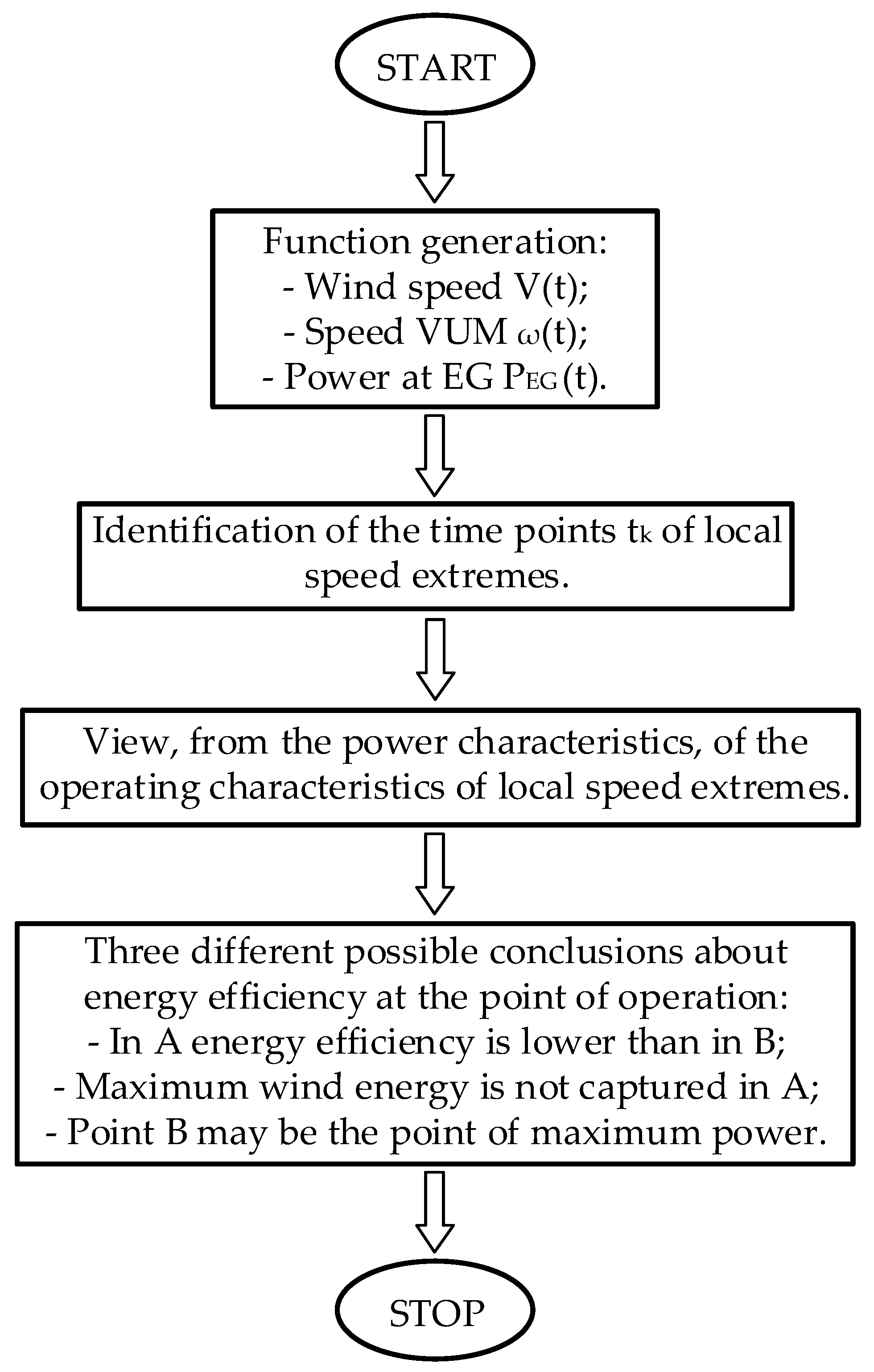
6. Algorithm for Determining Power Losses

The algorithm for visualizing the optimal energy zone consists of four steps. The first step is to collect the experimental data by recording the wind speed, power, and generator speed. In the second step, the time moments, t_ks, at which the speed, the function ω(t), has local extremes are identified and the turbine power is calculated. The third step is to extract from the experimental data the values for wind speed (v₁), and optimal MAV (ω_OPTIM), at time t_k. Finally, in step four, the conclusions about the power losses at the analyzed operating points are mentioned.

• Step 1—in the first step, the functions generated are the wind speed, v(t), mechanical angular speed, ω(t), power at EG, P_EG(t), presented in Figure 18;
• Step 2—in the second step, the time moments, t_ks, are identified at which the speed, the function ω(t), has local extremes, presented in Figure 19;
• Step 3—in the third step, the P_WT(ω) functions are displayed for the WT power characteristics, with the operating points defined by the local speed extremes (e.g., A and B), presented in Figure 20;
• Step 4—finally, in step four, conclusions are drawn about the energy efficiency of the operating points.

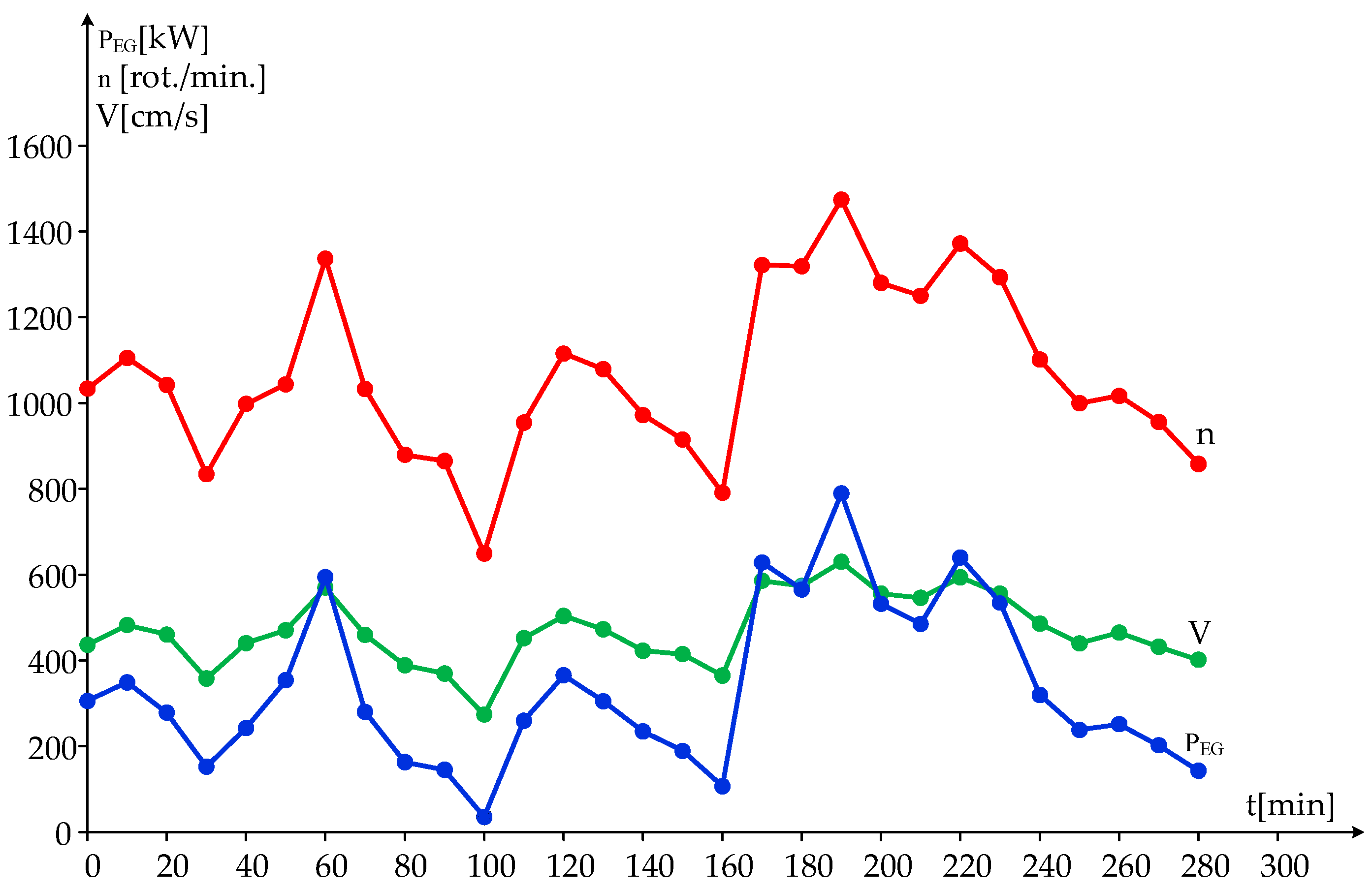
Figure 18. Time variation in wind speed, rotation speed, and power of electric generator.

Figure 18. Time variation in wind speed, rotation speed, and power of electric generator.

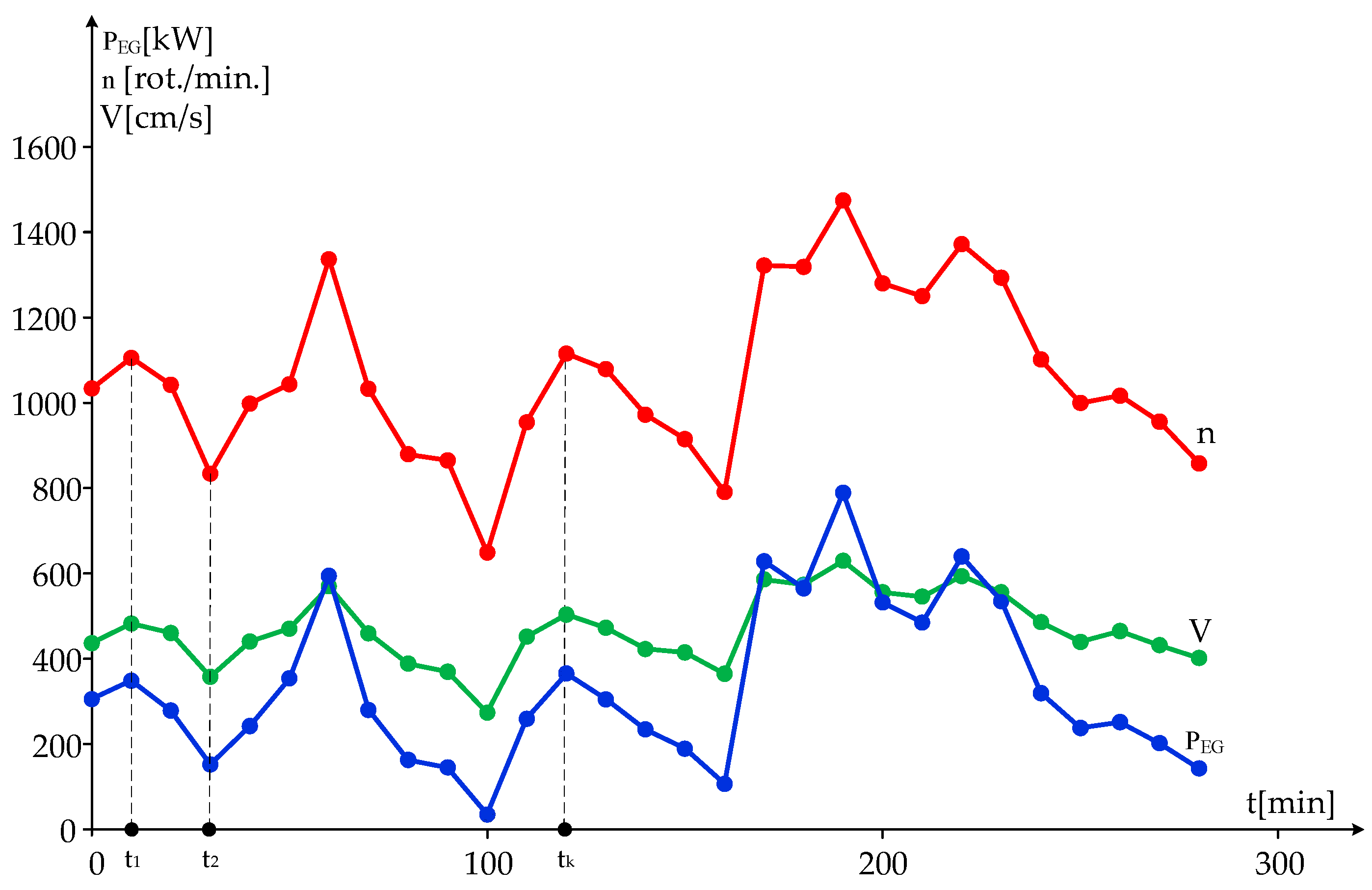
Figure 19. Identification of local speed extremes.

Figure 19. Identification of local speed extremes.

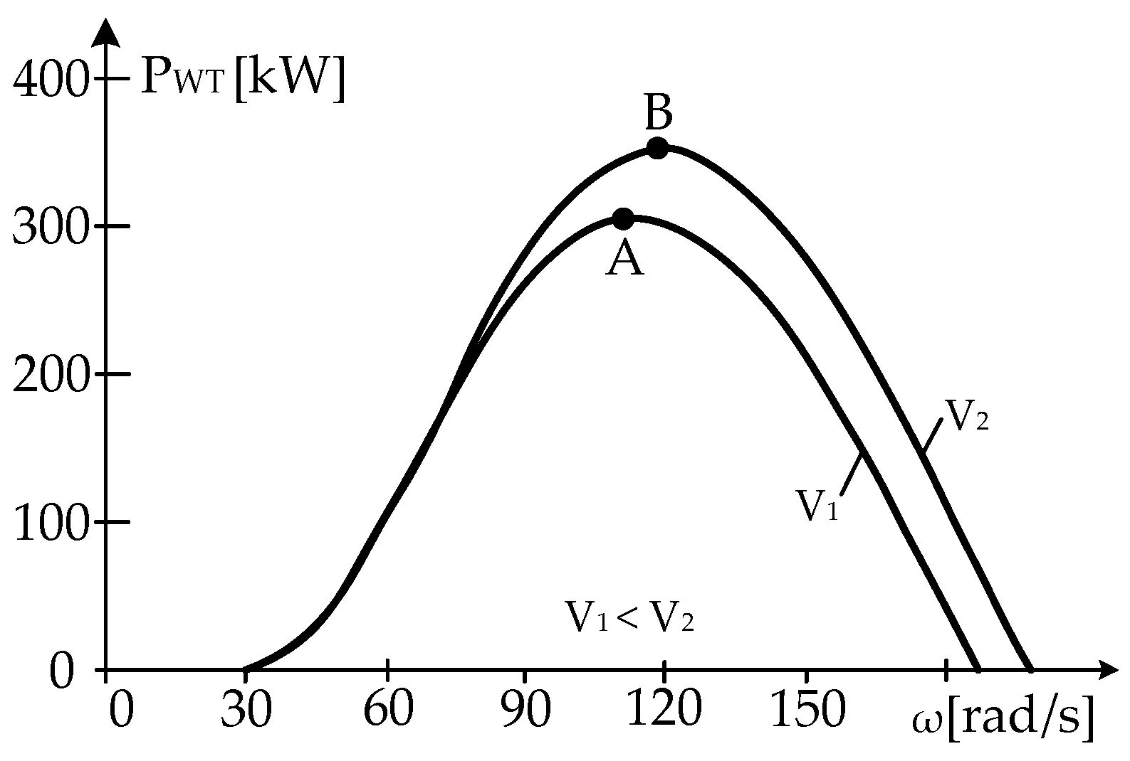
Figure 20. Operating points defined by local extremes A and B.

Figure 20. Operating points defined by local extremes A and B.

For example, only one of the following conclusions about the energy efficiency at the point of operation may be true:

• In A, the energy efficiency is lower than in B;
• In A, no maximum wind energy is captured;
• Point B may be the point of maximum power.

Figure 21 shows the algorithm used to determine the loss of power.

7. Discussion of the Findings

7.1. Operating Results

The results of this study are as follows:

• The local extremes of the speed, or the function ω(t), are obtained simply by recording the speed over time at a sampling step, ∆t, dependent on the value of the speed derivative of the wind, dv/dt, and the value of the moment of inertia, J;
• For the design of the control system, it is essential to know the exact dependence of the optimal MAV, ω_OPTIM, on the wind speed, v. This is easily determined from the mathematical model of the WT;
• The results obtained are used to determine the mathematical model of the WT, a useful model in control design;
• The visualization of the operating points makes it possible to estimate the power losses due to the incorrect value of the reference variable, ω_OPTIM, in the control system;
• In reality, the power losses are higher than the calculated ones, more than 48% (the value previously obtained from the existing experimental data). In the calculations, some operating points are considered as MPPs, which cannot be verified due to the lack of a wider range of speed values at the same wind speed value;
• On the power function graph, P_WT(ω, v), the operating points are located, and compared to the maximum power points, MPPs.

7.2. Fundamental Aspects

Through this study, the following relevant aspects can be highlighted:

• The certain aspects are as follows:
  • Determining the turbine power, P_WT, from equality with the power at the electric generator shaft, P_EG, at the local extreme points of the MAV, for the function ω(t);
  • At some operating points, the maximum wind energy is not captured, as shown in the experimental data by comparing the WT power values;
  • At the local extremes of mechanical angular velocity (MAV), for the function ω(t), the turbine power at the shaft is equal to the electric generator power at the shaft.
• The uncertain issues are as follows:
  • One of the operating points can be the MPP and it can capture the maximum primary wind energy;
  • But it is not known whether the range of speed values (MAV) contains the optimum zone (0.9–1.1)ω_OPTIM, including the MPP;
  • At the local extreme points of speed (MAV), for the function ω(t), it is possible that the speeds are equal to the optimal values.

7.3. Main Parameters and Selection Criteria

The analysis of the operating points defined by the local extremes of speed is characterized by the following:

1.

The zero value of the derivative of the mechanical angular velocity, dω/dt;

2.

The simplified form of the momentum equation

J · (dω/dt) = 0 = M_WT − M_EG

(95)

3.

The WT’s power equality with the EG in dynamic mode

J · (dω/dt) · ω = 0 = P_WT − P_EG; P_WT = P_EG

(96)

4.

It is not necessary to know the value of the equivalent moment of inertia, J, as the power given by the WT is equal to the power from the EG (which is obtained from the power delivered to the grid by dividing by the EG efficiency value).

The method presented provides the basis for a control system with reference measurements updated in real-time, which is particularly useful for capturing maximum wind energy, a method that does not exist in the literature.

In control design, the use of an incorrect value for the reference variable no longer ensures operation in the optimal MPP range, which is defined by the correct values for the reference variable to ensure the operation of the wind turbines in the MPP range.

The optimal parameter values are visualized during the operation of the wind turbine.

For a clear view of the maximum power, the initial prescribed value of the generator power, P_EG, must be much lower than the maximum value of the WT power, P_MAX, and the value of the wind speed at the initial time, v₀.

In physical systems with fixed power maxima over time (e.g., wind power systems operating at v = const.), it is not necessary to know the exact dependence of the optimal MAV, ω_OPTIM, on the wind speed and the Perturb and Observe Method, POM, can be applied.

In wind power systems operating at time-varying wind speeds, v ≠ const, the optimal MAV value changes over time, and due to the large mechanical inertia (large moment of inertia) the POM cannot be applied.

To obtain the most accurate view of the local extremes of the speed, the value of the sampling step, ∆t, should be as small as possible.

In conclusion, by estimating the wind speed and speed values at the electrical generator at a well-defined sampling step, ∆t, and at an initial MAV value, ω(0), below the optimal MAV value corresponding to the wind speed, the maximum power point of the WT can be identified.

In the present paper, the authors analyzed the variation in the wind speed at a wind turbine—a GE 2.5 MW 100— at Galbiori in the Dobrogea area, for which they recalculated the mathematical model based on the experimental data. Also, the dependence of the optimal mechanical angular speed on the wind speed—a reference quantity in the WT control system—was computed to achieve maximum wind energy capture. The optimal mechanical angular velocity was determined in the context of the dependence between maximum power and wind speed, and their time variations were compared with the real ones. The operating points resulting from the measurements were positioned on the power characteristics of the wind turbine and compared with those corresponding to the maximum power points, demonstrating that in most cases, the WT does not operate in the maximum power points.

8. Conclusions

In this paper, the local speed extremes were identified, and it was shown that in most cases, wind turbines do not achieve maximum power point tracking. By visualizing the operating points on the WT power curve, the resulting power losses were estimated. A control method with reference variables updated in real-time was presented, a method that does not exist in the literature. The results obtained are based on experimental data from wind turbines on the Romanian Black Sea coast—the Dobrogea area.

The research in this field is characterized by many gaps, such as a lack of relevant works aimed at determining the dependence of the optimal mechanical angular speed on the wind speed, and data from the technical book of wind turbines, having differences in time in operation, require a recalculation of the mathematical model based on measurements from where it operates. The aim of the research in this work was precisely to eliminate these gaps, in the sense that the power conversion coefficient must always be recalculated over time because the initial conditions have changed; the ratio λ, the ratio between the speed of the ends of the blades and the speed of the wind, a reference quantity in the control system, always has to be recalculated.

By analyzing the time variations in the MAV, the extreme points of the ω(t) function could be identified. For these local extremes, the derivative of the mechanical angular velocity is zero, dω/dt = 0, and the WT power in the dynamic mode at these operating points is equal to the power from the electric generator, P_WT = P_EG. The operating points, positioned on the WT power characteristics, were compared with those corresponding to the maximum power points. Future research should ensure that wind turbines operate at their optimum mechanical angular velocity, at the maximum power point of the turbine, by varying the load on the electrical generator as a function of wind speed. Thus, based on the experimental data, maximum wind energy capture can be achieved even with variable wind speeds over time. Furthermore, the visualization of the optimal area from an energy point of view, to locate the operating points of the WT compared to the maximum power point, allows for a much more precise determination of the energy yield. Additionally, a reliable mathematical representation of the turbine was established, and adjusted using data collected from the operational wind turbine, a model that underwent experimental validation. Moreover, a comparison of the optimal mechanical angular speed and the current mechanical angular speed was also visualized.