Short-Term Load Forecasting Method for Industrial Buildings Based on Signal Decomposition and Composite Prediction Model

Abstract

Accurately predicting the cold load of industrial buildings is a crucial step in establishing an energy consumption management system for industrial constructions, which plays a significant role in advancing sustainable development. However, due to diverse influencing factors and the complex nonlinear patterns exhibited by cold load data in industrial buildings, predicting these loads poses significant challenges. This study proposes a hybrid prediction approach combining the Improved Snake Optimization Algorithm (ISOA), Variational Mode Decomposition (VMD), random forest (RF), and BiLSTM-attention. Initially, the ISOA optimizes the parameters of the VMD method, obtaining the best decomposition results for cold load data. Subsequently, RF is employed to predict components with higher frequencies, while BiLSTM-attention is utilized for components with lower frequencies. The final cold load prediction results are obtained by combining these predictions. The proposed method is validated using actual cold load data from an industrial building, and experimental results demonstrate its excellent predictive performance, making it more suitable for cold load prediction in industrial constructions compared to traditional methods. By enhancing the accuracy of cold load predictions. This approach not only improves the energy efficiency of industrial buildings but also promotes the reduction in energy consumption and carbon emissions, thus contributing to the sustainable development of the industrial sector.

1. Introduction

With global warming and the escalating energy crisis, the issue of energy consumption in the construction industry has garnered significant attention worldwide in addressing energy and climate challenges. In particular, in rapidly urbanizing countries like China, where the construction industry is experiencing rapid growth, the cumulative energy consumption during the construction and operational lifecycle accounts for approximately one-third of the national energy consumption [1]. Among various contributors to building energy consumption, industrial buildings, due to their high operational intensity and complex usage requirements, have seen a continuous rise in their share of energy consumption with a growing demand [2]. In this context, the air conditioning system, as a piece of primary energy-consuming equipment in buildings, constitutes 40–60% of energy consumption in industrial buildings, making the enhancement of its energy efficiency a crucial avenue for reducing overall energy consumption in industrial buildings and achieving energy savings and emissions reduction [3,4]. To optimize energy usage efficiency, reduce consumption, and alleviate the burden on the power grid, many buildings have adopted energy-saving technologies, such as ice storage cooling. For example, based on ice storage cooling technology, energy systems in buildings can prepare cooling energy during off-peak periods and release it during high-demand periods, achieving low-cost utilization of building energy systems, optimizing energy usage efficiency, and reducing the burden on the power grid [5,6,7]. However, precise cooling load prediction is a key prerequisite for the efficient operation and energy optimization of ice storage cooling systems in buildings [8].

In the field of building cooling load prediction, current methods can be broadly categorized into two main types: those based on physical models and those driven by data [9]. Physical model-based methods typically employ simulation software, such as EnergyPlus 9.6.0 and TRNSYS 18.02, to simulate the thermal dynamics and energy consumption of buildings [10,11,12]. These methods often require skilled professionals to undertake complex modeling and extensive learning, resulting in relatively high time and manpower costs [13]. Moreover, for structurally complex and functionally intricate industrial buildings, constructing an accurate physical model is often impractical [14]. For instance, when simulating the energy consumption of large industrial complexes, various variables such as human traffic, equipment usage, natural lighting, internal heat sources, and more need to be considered. The interplay of these factors increases the difficulty and uncertainty of modeling [15].

With the continuous advancement of building information technology, a series of advanced data management systems, such as Building Information Modeling (BIM) and intelligent building management systems, are widely adopted. These systems systematically collect and store various data generated during the operation and maintenance of buildings [16,17]. Leveraging rich historical building energy data, data-driven methods based on machine learning algorithms or statistical analysis principles have achieved precise predictions of building energy consumption [18]. While data-driven methods based on statistical analysis principles are characterized by simplicity and computational convenience, they struggle to handle the high-dimensional data volume associated with enriched energy consumption data and personnel movement information. Subsequent research has extensively applied machine learning-based data-driven approaches to building load prediction [19]. Common machine learning prediction methods include Support Vector Machines (SVMs) [20,21,22], Artificial Neural Networks (ANNs) [23,24], and Deep Learning (DL) methods [25,26,27]. In the field of load prediction, various data-driven methods each play a unique role, synergistically enhancing the accuracy and efficiency of predictions.

Due to the influence of complex usage patterns, diverse load compositions, data uncertainty, climate variations, and human factors, the electric load prediction accuracy of industrial buildings is often low [28]. To address this issue, researchers have proposed methods for load prediction through time series forecasting, which is more effective in capturing nonlinear factors in load changes and reduces the need for feature data collection in regression predictions [29]. Random forests are highly robust in handling short-term fluctuating load data, effectively addressing random noise and outliers in the data. Meanwhile, deep learning, owing to its outstanding performance in handling long-term sequential data, enables accurate capture and prediction of load fluctuations caused by seasonal changes, weather patterns, or consumption behavior trends [30,31]. The flexible selection or combination of these models has become a crucial strategy for improving accuracy in load prediction research. In Karijadi et al.’s study, it was found that, in energy consumption prediction research, the RF model exhibits good performance in high-frequency data prediction when combined with data decomposition strategies, while the LSTM method achieves better accuracy in predicting low-frequency signals [32]. Liu et al. proposed a method that combines Empirical Mode Decomposition (EMD) with Support Vector Regression (SVR) for predicting office building energy consumption, demonstrating the effectiveness of combining signal decomposition methods with prediction models [33]. Swarm intelligence methods for parameter optimization of prediction models to enhance prediction accuracy have gained popularity in recent years. Pan et al. used Grey Wolf Optimizer (GWO) to search for LSTM hyperparameters, applying the GWO–LSTM model to predict the degradation trend of fuel pumps [34]. Liu et al. employed an improved Sparrow Search Algorithm (ISSA) to optimize the hyperparameters of the LSTM load prediction model, and experimental results indicated that the RMSE of this prediction model reached 3.35 [35]. Song et al. presented a WOA–BiLSTM model for predicting energy consumption in a Beijing hospital, showing enhanced accuracy and significant MAPE improvements [36]. Song et al. proposed a novel deep learning-based prediction framework, aTCN–LSTM, which integrates a gate-controlled multi-head temporal convolutional network and a sparse probabilistic self-attention mechanism with a BiLSTM network, demonstrating superior cooling load forecasting accuracy and effectiveness for HVAC systems optimization, validated through a 14-month study in a 51-story hotel [26]. Research indicates that BiLSTM, owing to its enhanced capabilities in both long-term and short-term memory, achieves superior predictive accuracy in complex data prediction scenarios, such as forecasting cold load and energy consumption. This enhanced performance is attributed to its more effective capture of the nonlinear dynamics inherent in time series data, marking a notable improvement over traditional LSTM and other conventional methods.

In summary, although some studies have employed integrated learning methods involving signal decomposition and swarm intelligence optimization, these methods have not effectively addressed the issue of low prediction accuracy caused by fluctuations in industrial building cold loads. Parameter errors in signal decomposition methods may result in the loss of information from parts of the original signal, and unimproved swarm intelligence methods can lead to local optimization problems, making it challenging to achieve the optimal signal decomposition effect. These issues contribute to a decrease in the accuracy of energy consumption predictions. Therefore, this paper proposes an industrial building cold load prediction method based on ISOA–VMD–RF–BiLSTM-attentionThe schematic illustration is shown in Figure 1. The SOA introduced by A. Hashim et al. [37] is selected for its excellent global search capability and fast convergence, making it suitable for solving complex multimodal optimization problems. Through enhancements using sine chaotic mapping initialization, adaptive inertia weight factors, and Levy flight strategy, ISOA is applied to optimize the parameters of the VMD signal decomposition method. This optimization yields the best decomposition result for cold load data in industrial buildings. Subsequently, signal analysis is conducted through a frequency spectrum, with high-frequency Intrinsic Mode Function (IMF) components and residuals input into the RF model for prediction, while low-frequency IMF components are input into the BiLSTM-attention model for prediction. The results of each component are summed to obtain the final prediction. Experimental results demonstrate that this model exhibits good performance in predicting cold loads in complex industrial buildings, facilitating the implementation of daytimez scheduling within industrial buildings, and promoting energy conservation and carbon reduction.

2. Theoretical Background

2.1. Data Preprocessing Model

2.1.1. Variational Mode Decomposition (VMD)

VMD (Variational Mode Decomposition) is an adaptive signal processing technique designed to address the challenges of endpoint ambiguity and mode size in signal decomposition. In comparison to traditional EMD methods, VMD demonstrates superior performance. This algorithm effectively decomposes complex signals into distinct modes, encompassing both low and high-frequency components, thereby mitigating the high complexity, nonlinearity, and non-smoothness inherent in time series data [38]. VMD employs an iterative optimization approach to adaptively determine the IMF of a signal based on its characteristics, providing enhanced flexibility and robust decomposition capabilities. The specific computational process is elucidated by the mathematical Equations (1)–(4), incorporating key equations for variational optimization modeling and estimating mode bandwidth. This renders VMD a potent tool for handling non-stationary signals and complex temporal data [39].

$${\min }_{\left\{a_k\right\},\left\{b_k\right\}}{\displaystyle \sum _k{\displaystyle \int {\left|\frac{\partial }{\partial t}\left((\delta (t)+j\pi t)\ast a_k(t)\right)e^{-j{b}_{k}t}\right|}^2}}dt\mathrm{s}.\mathrm{t}.{\displaystyle \sum _k{a}_k}=x(t)$$

(1)

In this Equation (1), $\left\{a_k\right\}$ represents a set of mode functions and $\left\{b_k\right\}$ represents their corresponding frequencies. The objective is to minimize the squared gradients of each mode function, fitting their linear combination to the input signal $x(t)$. The constraint ${\displaystyle \sum _k{a}_k}=x(t)$ ensures that the total sum of the linear combination of mode functions equals the input signal.

$$\begin{array}{l}L(\{a_k\},\{b_k\},\lambda )=\alpha {\displaystyle \sum _k{\displaystyle \int {\left|\frac{\partial }{\partial t}\left((\delta (t)+j\pi t)\ast a_k(t)\right)e^{-j{b}_{k}t}\right|}^2}}dt\\ +\frac{1}{2}{\Vert x(t)-{\displaystyle \sum _k{a}_k}(t)\Vert }^2+\langle \lambda (t),x(t)-{\displaystyle \sum _k{a}_k}(t)\rangle \end{array}$$

(2)

Equation (2) introduces the Lagrangian operator to update Equation (1), where $\lambda$ is the Lagrange multiplier. $\alpha$ is a weight parameter, which adjusts the modal function to fit the input signal. By adjusting the Lagrange multiplier, a better fit to the input signal is achieved, enhancing the accuracy of mode decomposition [40]. This updated equation plays a crucial role in the iterative process of the VMD algorithm, aiding the optimization algorithm in progressively approaching the optimal fit to the input signal.

$${\widehat{a}}_{n+1}^k(\omega )=\frac{\widehat{x}(\omega )-{\displaystyle \sum _{i\ne k}{\widehat{a}}_i}(\omega )+\widehat{\lambda }(\omega )/2}{1+2\alpha {(\omega -b_k)}^2}$$

(3)

$${\widehat{b}}_{n+1}^k=\frac{{\displaystyle {\int }_0^{\infty }\omega }{\left|{\widehat{a}}_k(\omega )\right|}^{2}d\omega }{{\displaystyle {\int }_0^{\infty }{\left|{\widehat{a}}_k(\omega )\right|}^2}d\omega }$$

(4)

Equations (3) and (4) represent the update steps of the VMD model. The numerator part represents the input signal minus half of the modal functions other than the current modal function and the Lagrange multiplier. The denominator contains a bandwidth adjustment term, where $\alpha$ is a weight parameter, $\omega$ is the frequency, and $b_k$ is the frequency of the current mode function, and where ${\widehat{a}}_{n+1}^k$ denotes the update of the k-th mode in the frequency domain and ${\widehat{b}}_{n+1}^k$ represents the corresponding frequency update. This iterative process utilizes the gradient of the optimization problem to progressively update the modes and frequencies.

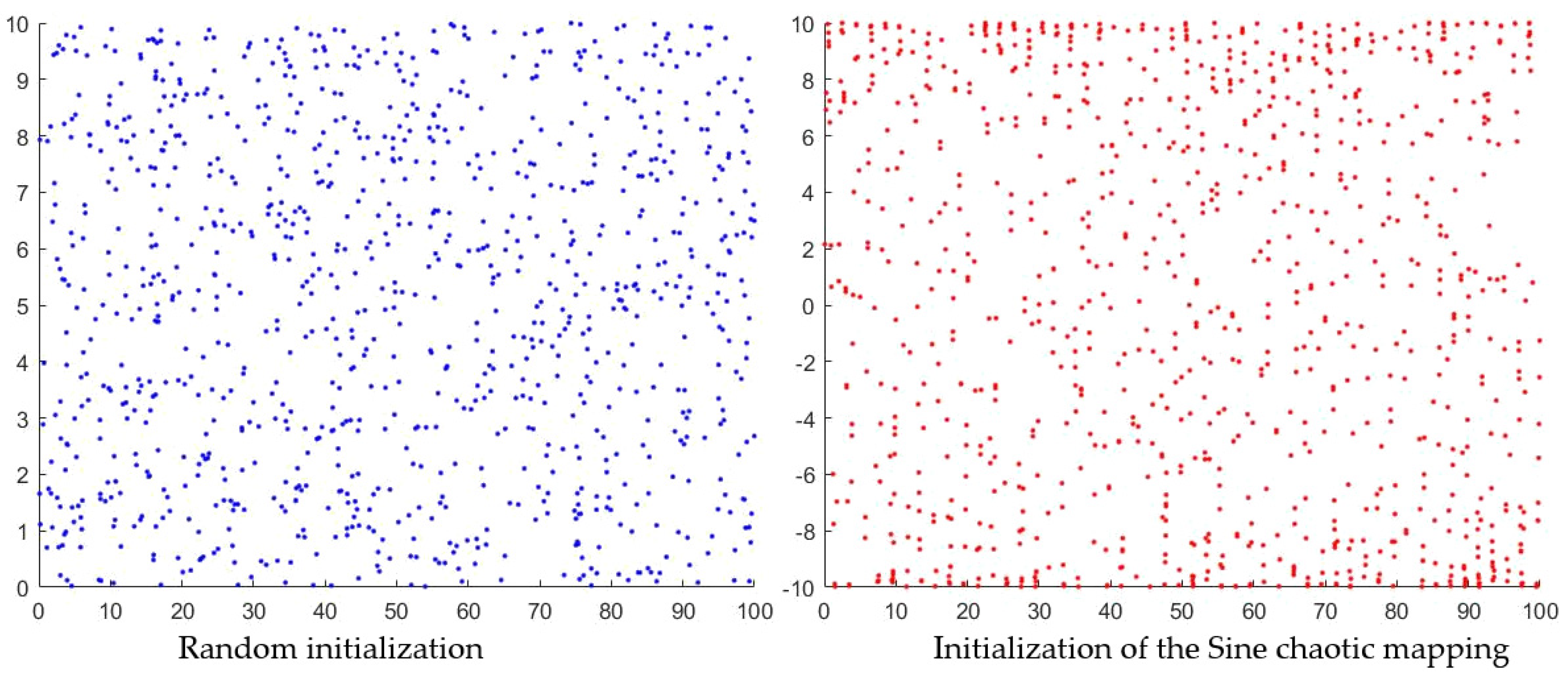
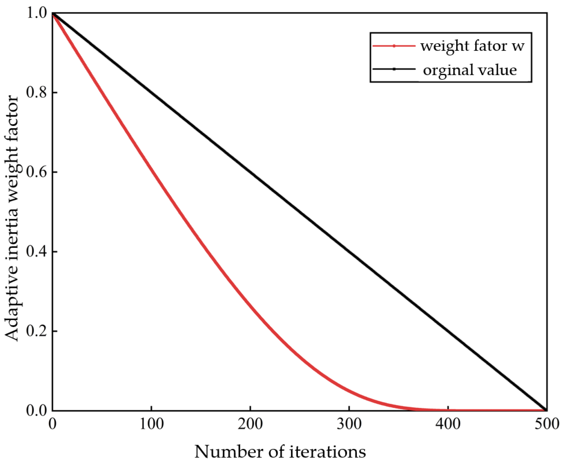
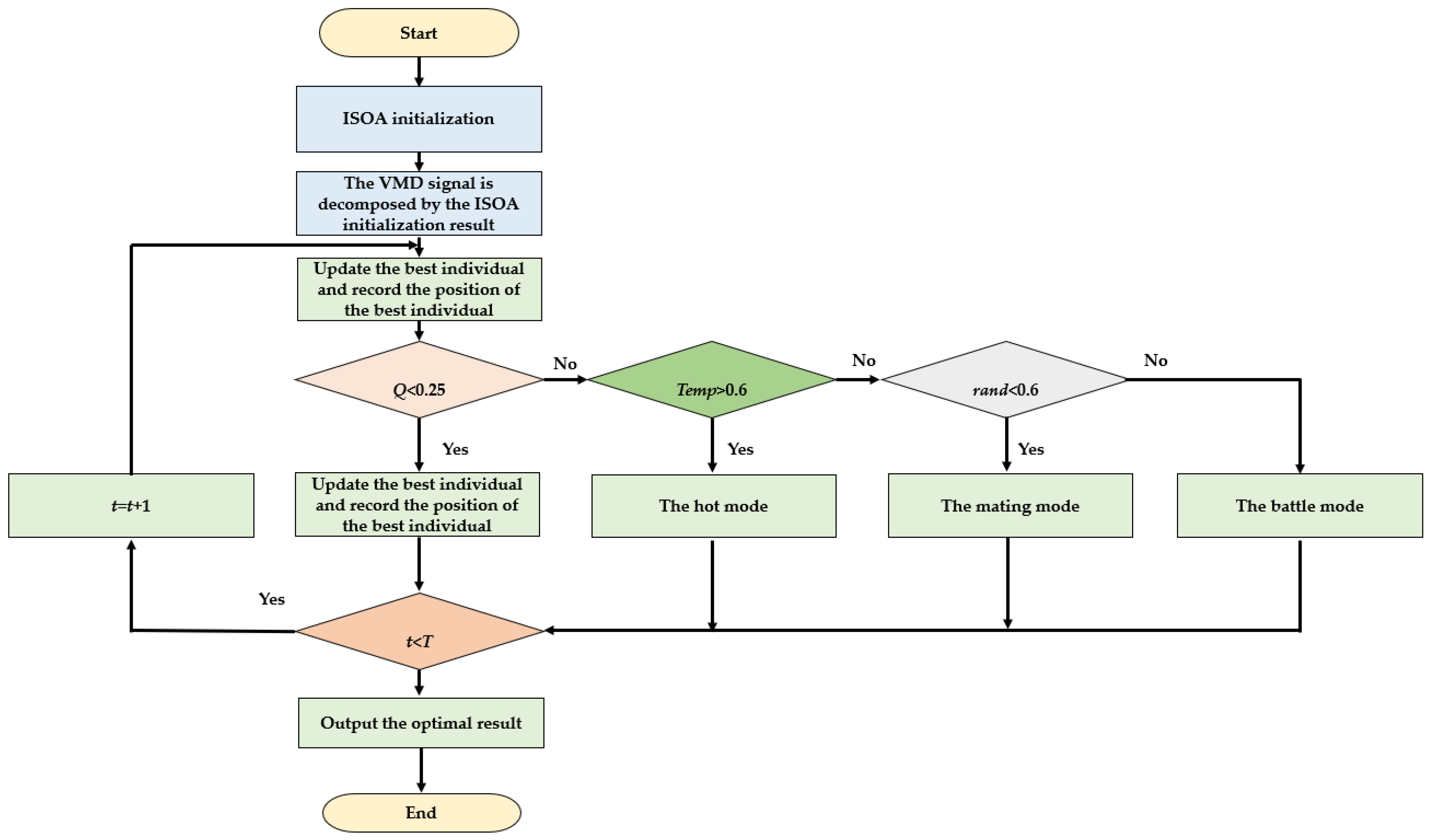
2.1.2. Improved Snake Optimization Algorithm (ISOA)

The SOA is a new intelligent optimization algorithm proposed by Hashim et al. that is a heuristic algorithm inspired by the collective behavior of snakes in biology. It simulates the behavior of snake groups in activities, such as food searching, migration, and collaborative behavior. The Snake Algorithm is primarily employed for solving optimization problems and signal-processing tasks [37].

The SOA is characterized by its simple structure and high flexibility; however, it faces challenges, such as susceptibility to local optima and slow convergence speed [41,42]. To overcome these drawbacks, the utilization of chaotic initialization enhances the diversity of the initial population, while the adaptive inertia weight factor helps balance exploration and exploitation during the search process. Additionally, the introduction of the Levy flight strategy strengthens global search capabilities and avoids local optima. The combination of these improvement measures aims to enhance the performance of the SOA algorithm, accelerate convergence speed, and increase the probability of finding the global optimum.

SOA has two phases: the exploration and exploitation phases, which are controlled by food quantity (Q) for conversion. When Q < 0.25, the SOA is in the exploration phase. On the contrary, when Q > 0.25, the algorithm is in the exploitation phase. Food quantity is calculated as follows:

$$Q=c_1\times \exp (\frac{t-T}{T})$$

(5)

where $t$ represents the current iteration, $T$ is the total number of iterations, and $c_1$ = 0.5. The initial population of the SOA is divided into two parts, denoted as $a$ and $b$ where $a$ represents the male population of snakes and $b$ represents the female population of snakes.

Exploration phase:

Equations (6)–(9) describe the process of position updating in the exploration phase of the SOA, where the snake swarm updates its positions based on fitness levels and random numbers. Firstly, $A_a$ and $A_b$ are calculated through exponential functions, where $fran{d}_a$ and $fran{d}_b$ represent fitness levels associated with a random number $rand$ and $f{i}_a$ and $f{i}_b$ are the fitness levels of individuals in the population. Next, the position update of the snake swarm is controlled by parameters related to the random number $rand$, and $Xran{d}_a(t)$ and $Xran{d}_b(t)$ are a randomly generated value that represents the current time a random number generated at time t. $c2$ is a constant used to control the adjustment amplitude of the algorithm. $Xub$ and $Xlb$ are the upper and lower bounds, respectively, used to limit the range of $X{i}_a(t+1)$ and $X{i}_b(t+1)$ and $c2$ = 0.05.

$$A_a=\exp \left(-fran{d}_a\cdot \frac{1}{f_{i,a}}\right)$$

(6)

$$A_b=\exp \left(-fran{d}_b\cdot \frac{1}{f_{i,b}}\right)$$

(7)

$$X{i}_a(t+1)=Xran{d}_a(t)\pm c2\cdot A_a\cdot ((Xub-Xlb)\cdot rand+Xlb)$$

(8)

$$X{i}_b(t+1)=Xran{d}_b(t)\pm c2\cdot A_b\cdot ((Xub-Xlb)\cdot rand+Xlb)$$

(9)

Exploitation phase:

In the Exploitation phase of the SOA, the snake swarm employs two different predation strategies, and the specific choice depends on $Temp$, and $rand$ is a random number that ranges from 0 to 1 (0 < $Temp$ < 1, 0 < $rand$ < 1); if $rand$ > 0.6, the snake swarm adopts the battle mode; otherwise, it uses the mating mode. When $Q$ > 0.25 and the temperature is greater than 0.6, the SOA is in the hot mode. In this case, the update of the snake swarm’s positions is determined by the following equation:

$$X{i}_j(t+1)=X_{food}\pm c3\cdot Temp\cdot rand\cdot (X_{food}-X{i}_j(t))$$

(10)

where $X{i}_j$ is the position of the individual (male or female), $X_{food}$ is the position of the best individuals, and $c3$ is constant and equals 2.

In the Cold mode of the SOA, when Q > 0.25 and the temperature is less than 0.6, the algorithm adopts a cold mode. In this mode, if $rand$ > 0.6, the snake swarm uses the battle mode, and its position update is determined by the following equation:

$$X{i}_a(t+1)=X{i}_a(t)+c3\cdot FA\cdot rand\cdot (Q\cdot X_{best,a}-X{i}_a(t))$$

(11)

$$X{i}_b(t+1)=X{i}_b(t)+c3\cdot FB\cdot rand\cdot (Q\cdot X_{best,b}-X{i}_b(t))$$

(12)

where $X{i}_a$ and $X{i}_b$ represent the positions of the $i$-th male and female individuals, respectively, and $X_{best,a}$ and $X_{best,b}$ are the best positions in the male and female groups. $FA$ and $FB$ are coefficients based on fitness levels.

$$FA=\exp \left(-\frac{fbes{t}_a}{f{i}_a}\right)$$

(13)

$$FB=\exp \left(-\frac{fbes{t}_b}{f{i}_b}\right)$$

(14)

The fitness levels of the best agents in the male and female groups are denoted as $fbes{t}_a$ and $fbes{t}_b$, respectively. Additionally, $fi$ represents the fitness level of the $i$-th agent in the population.

If $rand$ < 0.6, the SOA is in mating mode:

$$X{i}_a(t+1)=X{i}_a(t)+c3\times Ma\times \mathrm{rand}\times (Q\times X{i}_b(t)-X{i}_a(t))$$

(15)

$$X{i}_b(t+1)=X{i}_b(t)+c3\times Mb\times \mathrm{rand}\times Q\times (X{i}_a(t)-X{i}_b(t))$$

(16)

Equations (15) and (16) describe the mating properties of the snake swarm in mating mode, where $X{i}_a(t+1)$ represents the position update of the $i$-th male individual, and $X{i}_b(t+1)$ represents the position update of the $i$-th female individual at time $t+1$. $Ma$ and $Mb$ refer to the mating ability of males and females, respectively, and they can be calculated as follows:

$$Ma=\exp \left(-\frac{f{i}_b}{f{i}_a}\right)$$

(17)

$$Mb=\exp \left(-\frac{f{i}_a}{f{i}_b}\right)$$

(18)

During the hatching of the egg, the least-fit male, $X{\mathrm{poorest}}_a$ and the least-fit female, $X{\mathrm{poorest}}_b$ are substituted as follows:

$$X{\mathrm{poorest}}_a=X_{\mathrm{lb}}+\mathrm{rand}\times (X_{\mathrm{up}}-X_{\mathrm{lb}})$$

(19)

$$X{\mathrm{poorest}}_b=X_{\mathrm{lb}}+\mathrm{rand}\times (X_{\mathrm{ub}}-X_{\mathrm{lb}})$$

(20)

In the initialization phase of the Snake Algorithm, random number initialization leads to a simple random selection of the search space for the snake group, which fails to fully cover the search space. This results in low solution accuracy and insufficient mid-term global search capabilities. The main idea of chaotic optimization is to utilize the traversal and randomness characteristics of chaos. It maps variables to the value range within the chaotic variable space and linearly transforms the obtained solution back to the optimization variable space, thereby improving algorithm performance. Therefore, this paper adopts the sine map from chaotic mapping for the population initialization in the Snake Algorithm.

Figure 2 shows the population distribution comparison between random initialization and sinusoidal chaotic mapping initialization in the initial stage of the algorithm. The randomly initialized images show that the distribution of initial solution points in the search space is relatively scattered and concentrated, which may lead to insufficient exploration of the search space. On the contrary, the images of sinusoidal chaotic map initialization reveal a more uniform and widely dispersed population layout covering a larger range of the search space, which indicates that sinusoidal chaotic map initialization shows better global exploration potential and more efficient convergence ability.

The principle of the sine chaotic mapping is as follows:

$$C_i=\sin (\pi \times C_{i-1})$$

(21)

$$X_i\left(j\right)=\left(u{b}_j-l{b}_j\right)\ast C_i+l{b}_j$$

(22)

Here, $C_i$ is the sine mapping in the range [0, 1], and $u{b}_j$ and $l{b}_j$ represent the upper and lower bounds of the ith dimension, respectively. Equation (22) is the mathematical model of the selection space for the Bald Eagle Search Algorithm after initialization through the sine chaotic mapping.

The exploration phase of the Snake Algorithm is a crucial process determining the algorithm’s convergence speed. Due to a lack of effective control over the step size, the SOA is prone to deviate from the search direction, missing the optimal value range and leading to the algorithm becoming trapped in local optima. Therefore, in this study, the SOA algorithm is enhanced by incorporating an adaptive inertia weight factor. This adaptive mechanism dynamically adjusts the balance between exploration and exploitation, enhancing the convergence speed of the algorithm, preventing it from becoming trapped in local optima, reducing the need for manual parameter tuning, and strengthening the algorithm’s stability and adaptability. The adaptive mechanism automatically adjusts the weight based on the algorithm’s performance and the iteration process, making the optimization process more efficient and robust. The improved equation and comparison in Figure 3 are as follows:

$$\omega =\exp \left(\frac{ite{r}_{\max }+t}{ite{r}_{\max }-t}\right)$$

(23)

$$X_{i,new}=\omega \times rand\times X_{best}+d_x+d_y$$

(24)

where, $\omega$ represents the non-inertial weight factor, $ite{r}_{\max }$ denotes the maximum number of iterations, $t$ represents the current iteration count, and $X_{i,new}$ represents the updated individual position. Equation (24) suggests that the new position of individual i is determined by a combination of the non-inertial weight factor $\omega$, a random factor $rand$, the best position found so far $X_{best}$, and additional displacement terms $d_x+d_y$.

Levy flight is a type of random walk model characterized by the movement of a point in any dimensional space with a random length and direction, repeating this process. What makes Levy flight distinctive is the heavy-tailed distribution of step lengths, implying a certain probability of generating larger step lengths, potentially resulting in long-distance displacements. Additionally, each trajectory is different, adding randomness and diversity to the Levy flight. Introducing the Levy flight strategy during the development phase of the Snake Algorithm means incorporating the randomness of Levy flight into the algorithm to enhance its exploratory nature and flexibility. This introduction helps the algorithm explore solutions more extensively in the search space, improving its global search capability. The mathematical model of Levy flight is as follows:

$$lexy(x)~\lambda =t^{\lambda },1\le \lambda \le 1.5$$

(25)

where $x$ presents the random step length, and $\lambda$ is the exponent parameter. As the variance of Levy flight grows rapidly without bounds, introducing Levy flight during the development phase of the Snake Algorithm accelerates the search speed and effectively avoids becoming trapped in local optima.

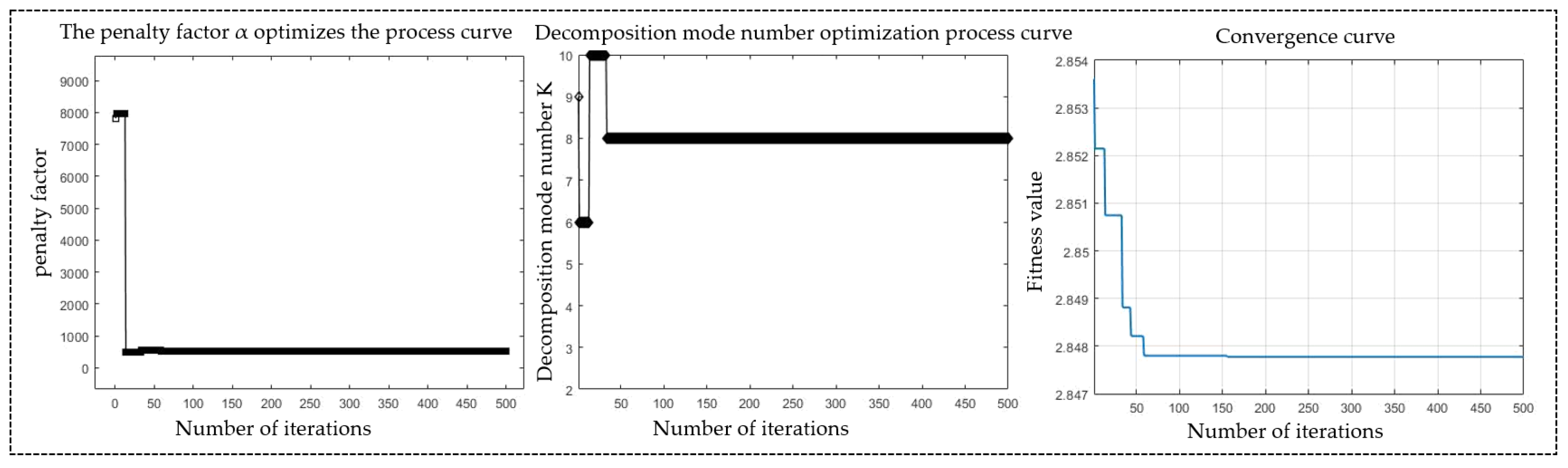
2.1.3. VMD Parameters Optimized Based on ISOA

The process of utilizing the ISOA to optimize VMD parameters is illustrated in Figure 4. VMD decomposes complex signals into a set of Intrinsic Mode Function (IMF) components, determined by the parameter K. In this process, the choice of K is crucial in adequately capturing all key features in the signal, while the regularization parameter α, controlling the bandwidth of each mode, affects the clarity and resolution of each mode. Setting K too small may result in the omission of essential information in the signal, while setting it too large may introduce irrelevant modes, increasing the complexity of the analysis. Similarly, a low value of α can lead to overly wide mode bandwidth, making the separation between modes unclear, while a high value may overly smooth the modes, causing detail loss.

This study employs the ISOA to optimize both the number of modes (K) and the regularization parameter (α). Envelop entropy is used as the fitness function, aiming to minimize it during the optimization process. In the context of the cooling load prediction, minimizing the envelop entropy serves as an adaptation function for optimizing the parameters in VMD, significantly enhancing the performance of the prediction model. By optimizing VMD parameters to reduce the envelope entropy of the signal, the preprocessing step becomes more effective in reducing noise and randomness in the original cooling load data, allowing for a more accurate capture of periodic and trending information related to the cooling load. This approach helps extract key features with predictive value for future load patterns, thereby improving overall prediction accuracy and laying a solid data foundation for subsequent prediction model accuracy.

2.2. Data Prediction Model

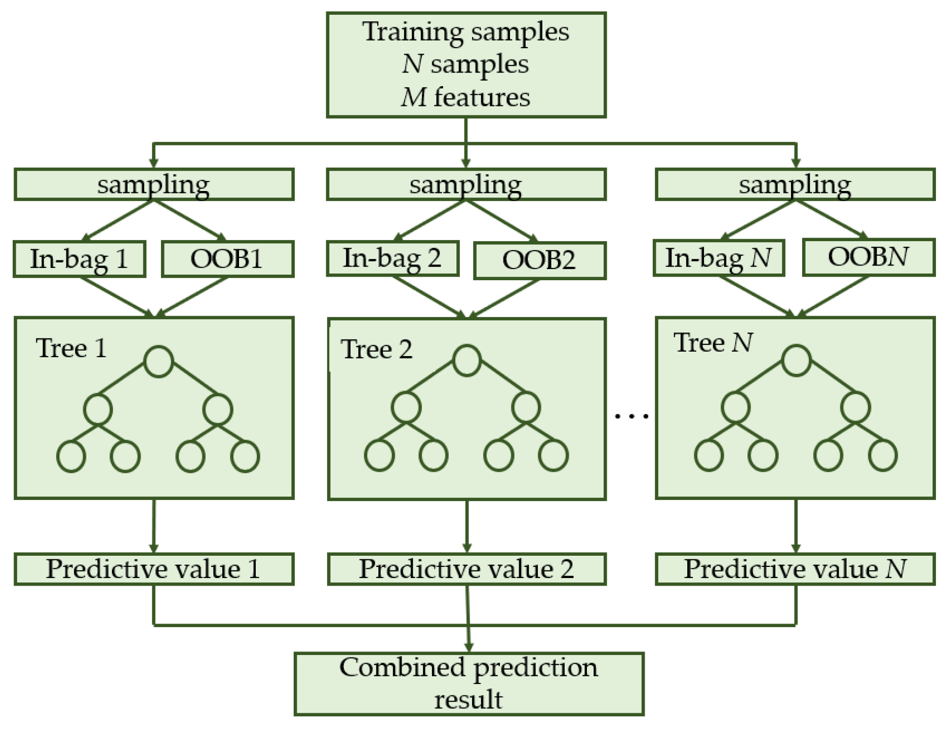
2.2.1. Random Forest (RF)

Random forest (RF) is a robust machine-learning approach capable of handling nonlinear relationships among multiple features and achieving exceptional predictive accuracy. This method demonstrates precision advantages in handling high-frequency non-linear data, such as IMF components. By combining multiple decision trees, RF flexibly models non-linear relationships, exhibits strong resistance to overfitting, accommodates numerous features and missing values, and is easily parallelizable, enhancing predictive performance. However, in practical applications, the choice of the most suitable model depends on specific problems and data characteristics; Figure 5 depicts the process of the random forest algorithm [43].

Initially, N training samples are randomly chosen from the original dataset using the bootstrap sampling technique, with each training set size approximately 2/3 of the original dataset. The remaining data not selected is known as out-of-bag (OOB) data, which is not utilized for training the regression trees. Subsequently, a classification regression tree is constructed for each training set, creating a forest comprising N decision trees. During the growth phase of each tree, m (m ≤ M) feature variables are randomly selected from the total M variables, and the optimal attribute is determined based on the minimum Gini coefficient to split the internal nodes. Finally, the predictions from the ensemble of N decision trees are combined. For classification problems, the mode of the voting results serves as the ultimate classification outcome. The optimal number of classification regression trees is determined through trial and error.

$${\epsilon }_{OOB}=\frac{{\displaystyle {\sum }_{i=1}^{N_{tree}}{(y_i-{y_i}^{OOB})}^2}}{N_{tree}}$$

(26)

$${R_{RF}}^2=1-\frac{{\epsilon }_{OOB}}{{{\sigma }_y}^2}$$

(27)

In the equation, ${\epsilon }_{OOB}$ represents the mean squared error, and $y_i$ and ${y_i}^{OOB}$ represent the true values and predicted values of the OOB data, respectively. ${\sigma }_y$ and $R_{RF}$ are the variance and correlation coefficient of the predicted values of the OOB data, respectively.

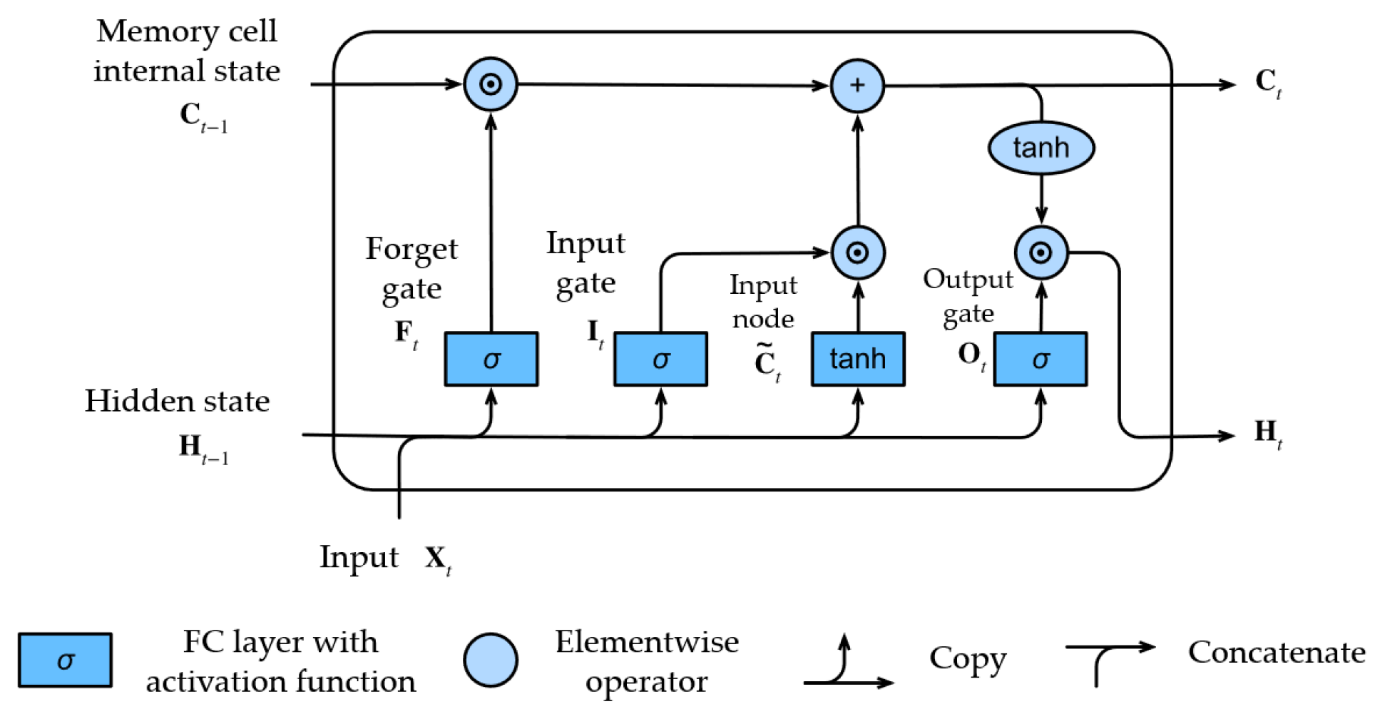
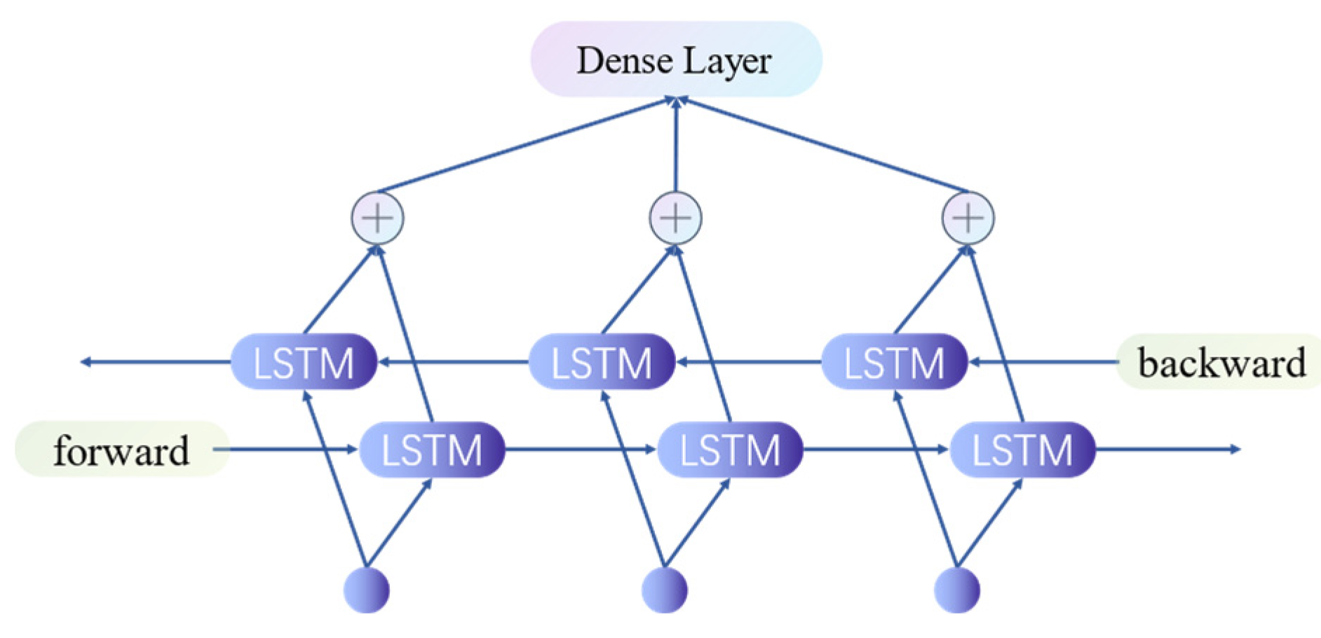
2.2.2. Bidirectional Long Short-Term Memory (BiLSTM)

BiLSTM (Bidirectional Long Short-Term Memory) is a neural network model designed for processing sequential data, and it is a variant of the Long Short-Term Memory (LSTM) network [44]. LSTM is a special type of Recurrent Neural Network (RNN) designed to address issues such as gradient vanishing and exploding gradients in traditional RNNs, with its specific structure illustrated in Figure 6.

The main characteristic of BiLSTM is its ability to consider both past and future information of the input sequence simultaneously [45]. Typically, traditional RNNs or unidirectional LSTMs can only utilize forward information, while BiLSTM introduces an additional backward layer, enabling the network to capture context before and after each time step in the sequence [46].

The structure of BiLSTM consists of two independent LSTM layers, one for processing the forward sequence and another for processing the backward sequence. Each LSTM unit has a memory cell and three gates (input gate, forget gate, and output gate), contributing to the model’s ability to remember long-term dependencies. At each time step, the forward LSTM and backward LSTM independently process the input sequence, and their outputs are then concatenated to form the final BiLSTM output, as depicted in Figure 7 of BiLSTM.

$$i_t=\sigma (W_{ii}{x}_t+b_{ii}+W_{hi}{h}_{t-1}+b_{hi})$$

(28)

$$f_t=\sigma (W_{if}{x}_t+b_{if}+W_{hf}{h}_{t-1}+b_{hf})$$

(29)

$$g_t=\tanh (W_{ig}{x}_t+b_{ig}+W_{hg}{h}_{t-1}+b_{hg})$$

(30)

$$c_t=f_t\cdot c_{t-1}+i_t\cdot g_t$$

(31)

$$o_t=\sigma (W_{io}{x}_t+b_{io}+W_{ho}{h}_{t-1}+b_{ho})$$

(32)

$$h_t=o_t\cdot \tanh (c_t)$$

(33)

where $x_t$ is the input at the $t$-th time step of the input sequence. $i_t$, $f_t$, $g_t$, and $o_t$ are the compute equations for the input gate, the forget gate, and the output gate, respectively. $g_t$ and $c_t$ are candidate memory cells and cell states, respectively. $h_t$ and $h_{t-1}$ are the final outputs of the network at the current time and the previous time, respectively. $W$ and $b$ are the weight matrix and bias of the three gating and cell states, respectively. $\sigma (·)$ is the sigmoid activation function, and $\tanh (·)$ is the hyperbolic tangent activation function.

2.2.3. Attention Mechanism (AM)

The Attention Mechanism is a technique designed to enhance the focus of deep learning models on different segments of input sequences. Initially introduced in the field of Natural Language Processing, particularly in machine translation tasks, its primary advantage lies in allowing models to dynamically attend to various parts of the input sequence during the generation of outputs, as opposed to treating the entire sequence with a fixed-weight approach [36].

The core concept of the AM involves calculating a weight distribution for each output generated by the model, indicating the relative importance of different positions within the input sequence. This weight distribution is computed by associating a query with the information at each position in the sequence. Consequently, the model, when generating each output, can dynamically adjust its focus based on the current context. Overall, the widespread application of the AM in deep learning provides models with a more flexible and precise modeling capability.

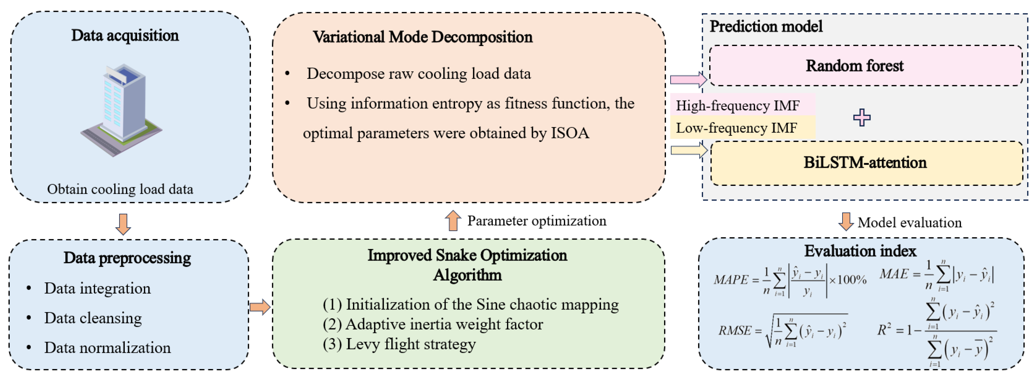
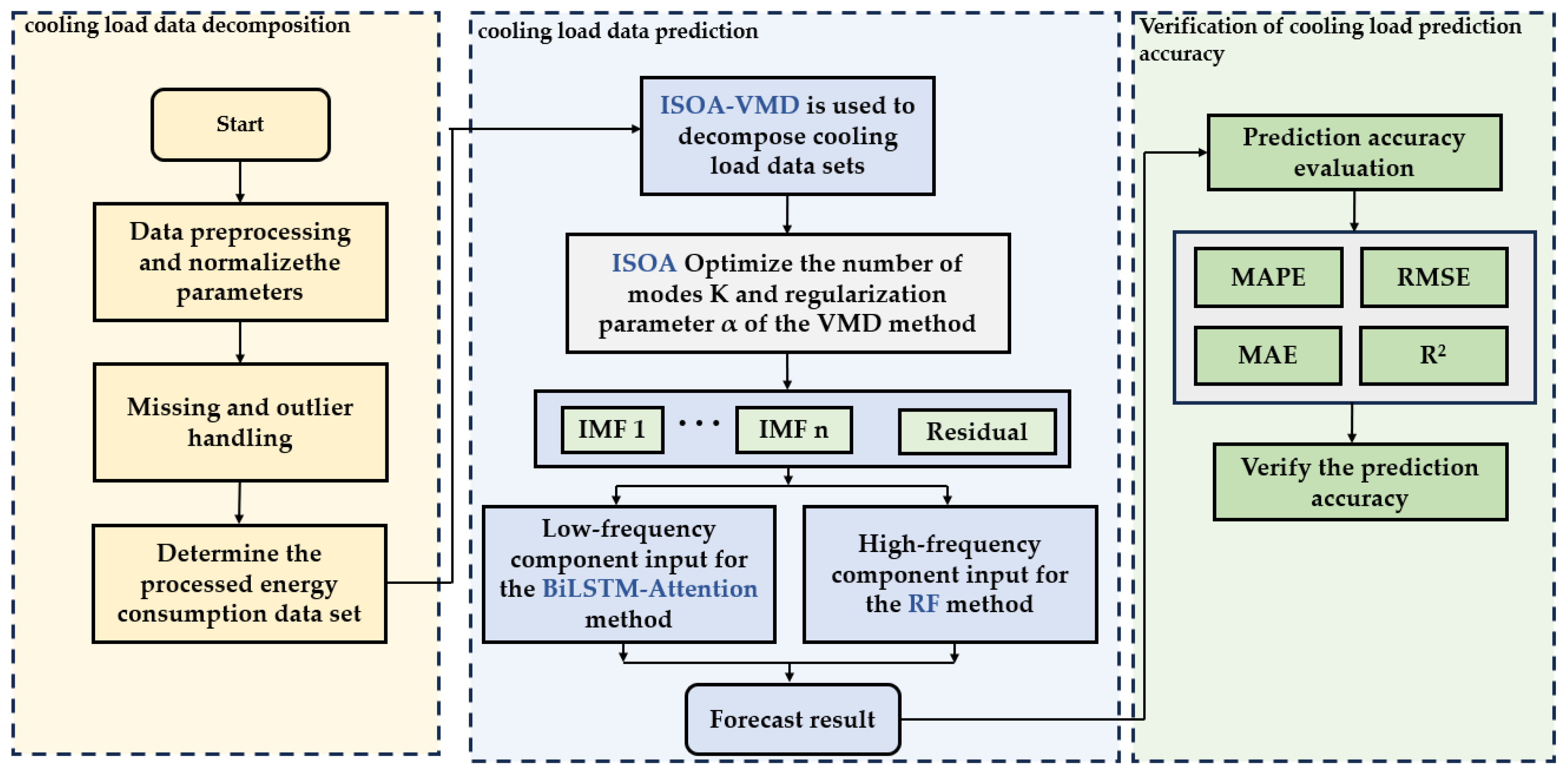
3. Framework of the Proposed Method

This study introduces an integrated learning approach combining ISOA, VMD, RF, and BiLSTM-attention. The first step involves the decomposition of cooling load data, where ISOA optimizes the number of modes (K) and the regularization parameter (α) in the VMD algorithm to obtain the VMD energy consumption decomposition result with the minimum envelope entropy. The second step focuses on cooling load prediction. RF is effective in capturing instantaneous and complex fluctuation patterns in high-frequency time series data, making it suitable for high-frequency fluctuating data. On the other hand, BiLSTM-attention excels in capturing long-term dependencies and global trends. Therefore, the decomposed cooling load spectrum, high-frequency IMF components, and residuals are inputted into the RF method, while low-frequency IMF components are inputted into the BiLSTM-attention method for prediction. The final cooling load prediction result is obtained by summing up the individual predictions. The flowchart of this method is illustrated in Figure 8.

The proposed cooling load prediction framework provides an efficient and accurate method for cooling load prediction by combining the unique advantages of ISOA, VMD, RF, and BiLSTM-attention. By optimizing VMD parameters, ISOA ensures that the data decomposition process can reveal the inherent characteristics and dynamic change rules of cooling load data, thus improving the basic quality of prediction. Random forest (RF) is excellent at predicting high-frequency volatility data and capturing instantaneous and complex patterns in the data. BiLSTM-attention, on the other hand, focuses on capturing long-term dependencies and global trends in data, which works well for low-frequency data. By integrating these techniques, the method can not only handle and predict subtle fluctuations in cooling load data but also accurately grasp and predict long-term trends, significantly improving the accuracy and robustness of the forecast.

4. Experimental Design

4.1. Data

This research collected cold load data for an industrial building in the Hebei province, China. The building is mainly used for the manufacturing and assembly of electronic products. It houses heavy industrial production workshops, light industrial assembly areas, and supporting office spaces. Heavy industry production workshops mainly involve high-energy consumption processes, such as raw material treatment, machining, assembly and welding, and surface treatment, and the cooling load in this area is high in the production stage. The assembly area and office area of the light industry focus on precision assembly, testing, and quality control of electronic components and small mechanical parts, emphasizing temperature and humidity control and clean air quality to ensure product quality and operator comfort and safety.

The building details are shown in

Table 1. Physical characteristics of the industrial building.

Building Physical Characteristic	Detailed Information
Building height	45 m
Building footprint	28,000 Square meter
Building air conditioning coverage	75%
Building insulation system	Polystyrene foam and polyurethane foam

. Considering the cold winters and hot summers in Hebei Province, the building has also been specially designed with an efficient insulation system, including the use of high-performance insulation materials and double glazing, to reduce energy consumption while maintaining the comfort of the indoor environment. The building design incorporates efficient ventilation and an intelligent air conditioning system to cope with extreme weather fluctuations, ensuring that the cold load remains stable at approximately 1000 kW to 2000 kW. This guarantees production efficiency and employee comfort.

The industrial building operates flexibly throughout the year, with typical operating hours from 7:00 AM to 9:00 PM; the cooling load data sampling interval is 1 h. In particular, during the hot summer months, the air conditioning system adjusts intelligently based on actual temperature and humidity to maintain optimal indoor conditions for production. As a result, the cold load exhibits distinct temporal characteristics, as illustrated in Figure 9.

4.2. Evaluation Metrics

To validate the predictive performance of the ISOA–VMD–RF–BiLSTM-attention model, the Mean Absolute Percentage Error (MAPE), Root Mean Square Error (RMSE), Mean Absolute Error (MAE), and Coefficient of Determination (R²) were selected as the primary evaluation metrics for assessing the model’s predictive accuracy.

These four evaluation indexes provide a comprehensive research method for the accuracy evaluation of industrial building cooling load prediction. MAPE visually shows the average difference between predicted and actual values in percentage terms but can be sensitive to outliers, which can affect the accuracy of the results. RMSE focuses on large prediction errors and helps to understand significant deviations in predicted values. While the MAE provides a robust measure of the average error level for all predictions, it is very resilient to extreme values. Finally, the R² statistic is used to judge the ability of the model to explain the variance of the target variable. The closer the value is to one, the stronger the explanatory power is. The evaluation index equation and description are shown in

Table 2. Evaluation index description.

Evaluation Index	Formula	Description
MAPE	$\frac{1}{n}{\displaystyle \sum _{i=1}^n\left|\frac{{\widehat{y}}_i-y_i}{y_i}\right|}\times 100\%$	Calculates the average of the absolute differences between predicted and actual values, divided by actual values, expressed as a percentage.
RMSE	$\sqrt{\frac{1}{n}{\displaystyle \sum _{i=1}^n{\left({\widehat{y}}_i-y_i\right)}^2}}$	Measures the square root of the average squared differences between observed and predicted values.
MAE	$\frac{1}{n}{\displaystyle \sum _{i=1}^n\left|y_i-{\widehat{y}}_i\right|}$	Computes the average of the absolute differences between observed values and model predictions.
R2	$1-\frac{{\displaystyle \sum _{i=1}^n{\left(y_i-{\widehat{y}}_i\right)}^2}}{{\displaystyle \sum _{i=1}^n{\left(y_i-\overline{y}\right)}^2}}$	Indicates the proportion of the variance in the dependent variable that is predictable from the independent variable.

.

${\widehat{y}}_i$ is the predicted value of the i-th sample of the test set, $y_i$ is the true value of the i-th sample in the test set, n is the total number of samples, and $\overline{y}$ is the average of the predicted actual values.

4.3. Experimental Settings

This study proposes an improvement to the SOA resulting in ISOA by incorporating sine chaotic mapping initialization, an adaptive inertia weight factor, and the Levy flight strategy. This method optimizes the number of decompositions and penalty factors in the VMD signal decomposition process, achieving the optimal decomposition for industrial building cooling load data. Subsequently, signal analysis is performed using the spectrum, where high-frequency IMF components and residuals are inputted into the RF model for prediction, and low-frequency IMF components are inputted into the BiLSTM-attention model for prediction. The results of each component are then summed to obtain the final prediction.

The combined prediction model proposed in this study is implemented in Python on a system running the Windows 11 operating system with an Intel Core i9-12400 processor @ 3.00 Hz. This processor offers high computational performance, contributing to the efficiency and accuracy of the model during execution. Experimental results demonstrate the model’s effectiveness in predicting the cooling load of complex industrial buildings.

5. Results and Discussion

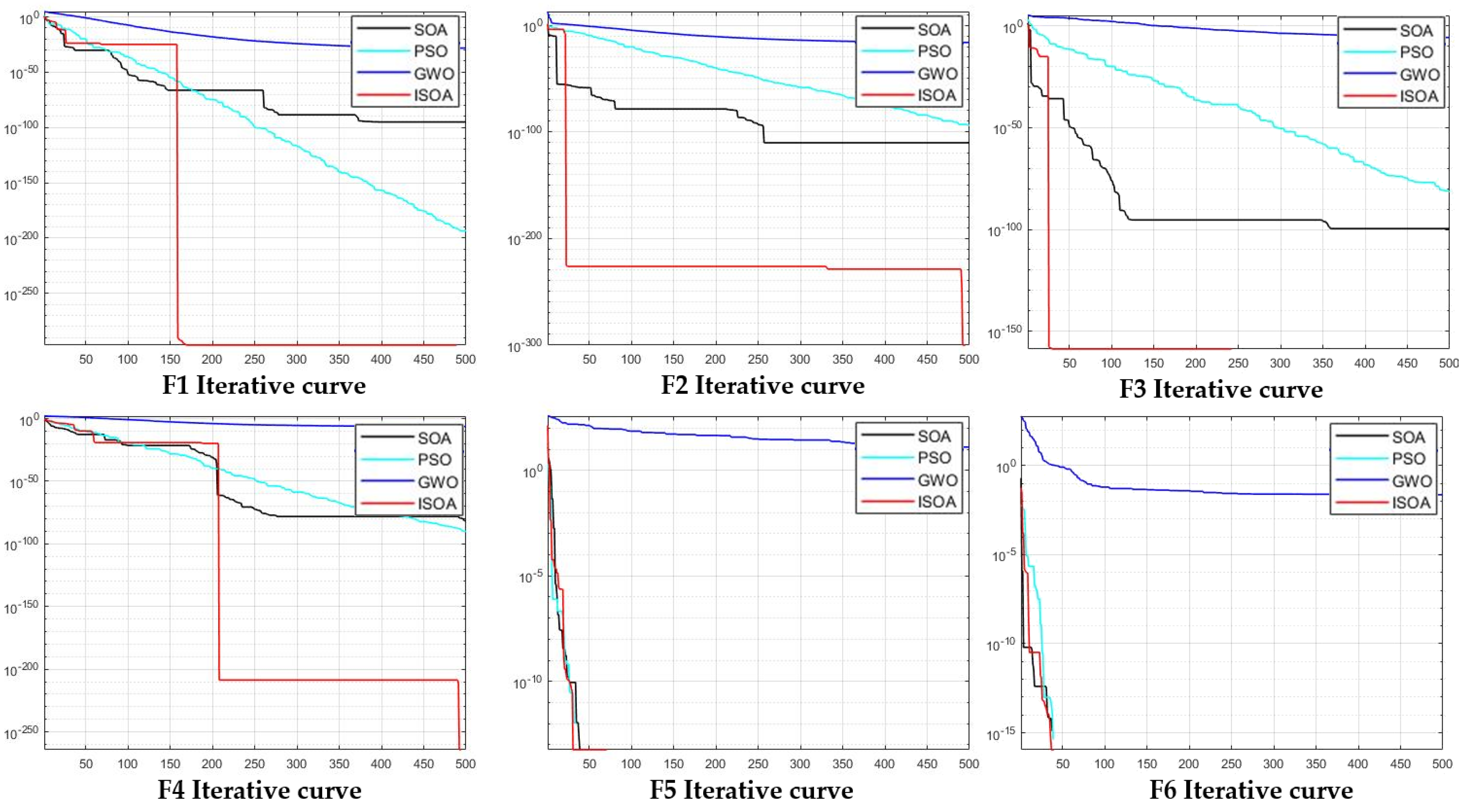
5.1. ISOA Performance Verification

Based on the algorithm improvement strategies described in Chapter 2, this paper proposes the ISOA with a hybrid strategy. To assess the advantages of this improvement compared to other algorithms, six test functions are selected for performance comparison between other optimization algorithms and ISOA. Functions F1 to F4 are single-peaked functions, which are suitable for testing the global search capabilities of algorithms and are easy to analyze. Functions F5 and F6 are high-dimensional multi-peaked functions, simulating complex real-world problems and testing the performance of algorithms in finding global optimal solutions. The specific expressions, domains, and optimal values of the test functions are provided in

Table 3. Details of the test functions.

Function	Analytic Expression	Dim	Initial Range	Optimal Value
$F_1$	$f\left(x\right)={\displaystyle {\sum }_{i=1}^n{x}_i^2}$	30	[−100, 100]	0
$F_2$	$f\left(x\right)={\displaystyle {\sum }_{i=1}^n\left|x_i\right|+}{\displaystyle {\prod }_{i=1}^n\left|x_i\right|}$	30	[−10, 10]	0
$F_3$	$f\left(x\right)={{\displaystyle {\sum }_{i=1}^n\left({\displaystyle {\sum }_{j=1}^i{x}_j}\right)}}^2$	30	[−100, 100]	0
$F_4$	$f\left(x\right)=\max \left\{\left|x_i\right|,1\le i\le n\right\}$	30	[−100, 100]	0
$F_5$	$f\left(x\right)={\displaystyle {\sum }_{i=1}^n\left[x_i^2-10\cos \left(2\pi x_i\right)+10\right]}$	30	[−5.12, 5.12]	0
$F_6$	$f\left(x\right)=\frac{1}{4000}{\displaystyle {\sum }_{i=1}^n{x}_i^2}-{\displaystyle {\prod }_{i=1}^n\cos \left(\frac{x_i}{\sqrt{i}}\right)}+1$	30	[−600, 600]	0

. The ISOA algorithm proposed in this paper is compared with Particle Swarm Optimization (PSO), Grey Wolf Optimization (GWO), and the unimproved SO. The parameter settings are detailed in

Table 4. Parameter Settings of the optimization algorithm.

Algorithm Name	Basic Setup	Parameter Setting
SOA	$n=40$ $ite{r}_{\max }=500$	$SL=0$, $SS=0.1$, $N_P=0.1$
PSO		$w=0.5$
GWO		${\alpha }_{\min }=0$, ${\alpha }_{\max }=2$
ISOA		$SL=0$, $SS=0.1$, $N_P=0.1$

.

Figure 10 displays the iteration curves for F1–F6, indicating that ISOA exhibits superior optimization accuracy and speed compared to other optimization algorithms across the four test functions. Additionally, in the initial stages of the iterations, it is evident that the improved ISOA method, incorporating sine chaotic mapping initialization, adaptive inertia weight factor, and Levy flight strategy, possesses strong randomness and favorable distribution characteristics, thereby enhancing performance and convergence speed. Notably, it demonstrates significant advantages in the optimization of single-peaked functions. For F5–F6, the improved ISOA method consistently and rapidly stabilizes to the optimum, unaffected by the characteristics of multi-peaked test functions. This underscores that the ISOA method yields higher precision in obtaining optimal solutions across all test functions. The introduced ISOA algorithm in this study showcases outstanding global search capabilities and robustness, with the improved algorithm exhibiting remarkable performance in optimization, providing robust support for the parameter optimization of the VMD method.

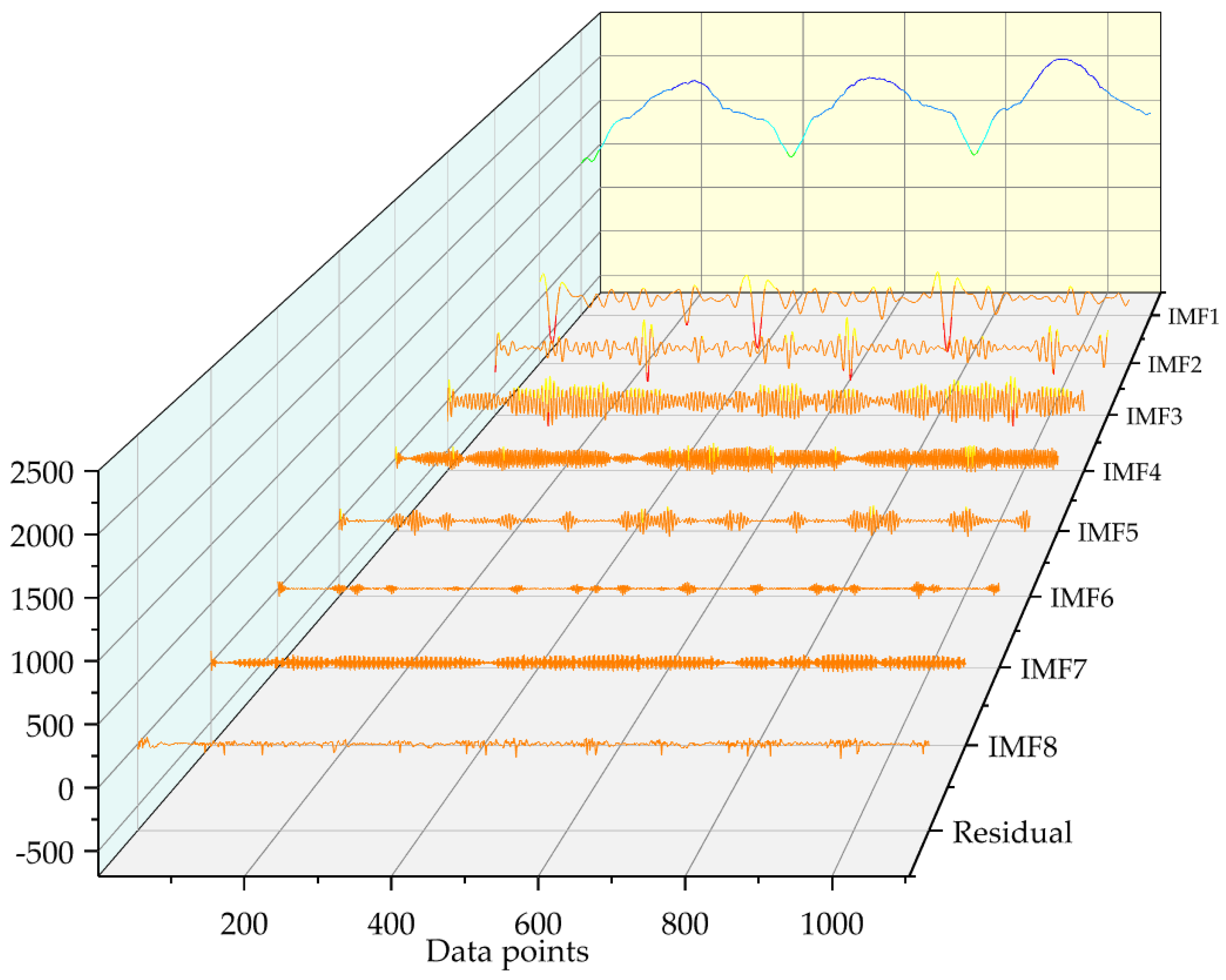
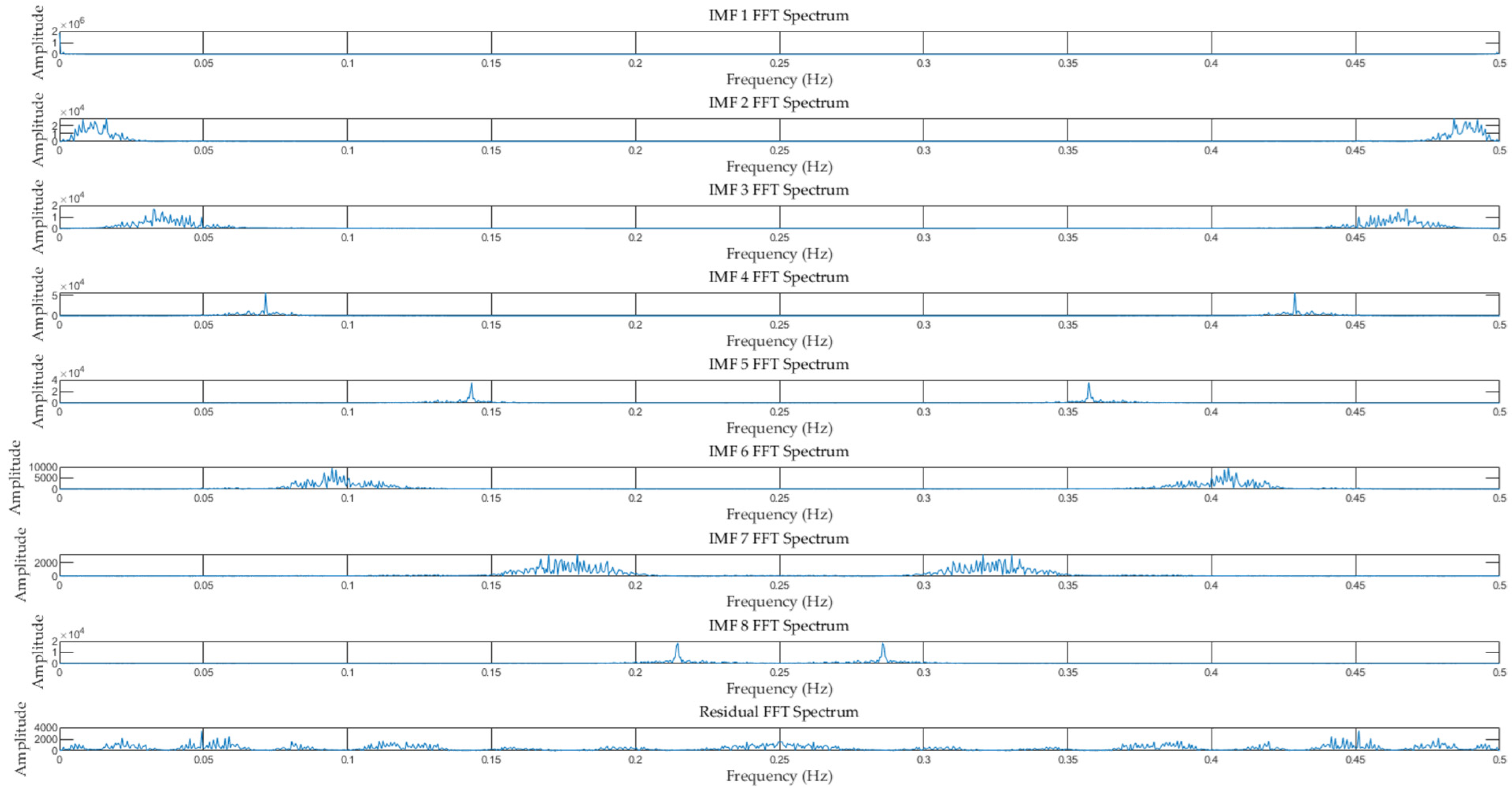
5.2. ISOA-VMD Cooling Load Data Signal Decomposition

To enhance the quality of the cooling load data and mitigate the impact of noise, this study employs ISOA–VMD for decomposing the cooling load data. The optimized parameters for the VMD method include two penalty factors and the number of decomposed IMFs, denoted as K. The range for K is [3, 10], and the penalty factors fall within the range of [100, 8000], exclusively as integers. Subsequently, the ISOA method optimizes the parameters of VMD with the minimum envelope entropy as the fitness function. As shown in Figure 11, at approximately 10 iterations, the penalty factors reach optimal values, while at approximately 50 iterations, both the fitness function and K achieve optimal values. The final number of IMF components is determined to be eight, resulting in eight IMF components and one residual.

As depicted in Figure 12 and Figure 13, these figures illustrate the ultimate decomposition results and spectrogram obtained by the ISOA–VMD method for cooling load data. The spectrogram reveals that the decomposition method exhibits effective performance. Combining the spectrogram, IMF2, IMF3, IMF4, and IMF6 are defined as high-frequency IMF components, which are input into the BiLSTM-attention model for prediction. Subsequently, IMF1, IMF5, IMF7, and IMF8 are defined as low-frequency IMF components, input into the RF model for prediction. Ultimately, this combination achieves the accurate prediction of cooling load, serving the intended purpose.

5.3. Performance Validation of the Model

To demonstrate the superiority of the proposed combined forecasting model ISOA–VMD–RF–BiLSTM-attention, this study conducts a comparative analysis with five algorithms, including RF, VMD–RF, VMD–RF–BiLSIM-attention, SOA–VMD–RF–BiCRU, and SOA–VMD–RF–BiLSIM-attention. The actual cooling load prediction error curves of the proposed method and the comparative methods are illustrated in Figure 14. In order to further verify the effectiveness of the model, this paper also collected the cooling load data of another industrial building to verify the effectiveness of the model. The prediction error results are shown in Figure 15. It is observed that the prediction error of the single RF method is relatively large, attributed to poor data quality resulting from noise. The significant reduction in prediction error with the VMD–RF method demonstrates the effectiveness of signal decomposition applied to forecast data. The comparison between SOA–VMD–RF–BiCRU and SOA–VMD–RF–BiLSIM-attention suggests that, compared to BiLSTM-attention, BiCRU may have drawbacks, such as higher computational complexity, increased parameter volume, and greater training difficulty, leading to an increase in prediction error.

Table 5. Cooling load Prediction accuracy evaluation metrics comparison table (A).

Model	MAE	MAPE	RMSE	R2
ISOA-VMD-RF-BiLSIM-attention	58.71	0.042	88.34	0.938
SOA-VMD-RF-BiLSIM-attention	59.29	0.043	94.99	0.927
SOA-VMD-RF-BiCRU	57.38	0.046	99.21	0.921
VMD-RF-BiLSIM-attention	63.88	0.047	100.32	0.918
VMD-RF	77.72	0.049	123.69	0.876
RF	118.38	0.062	171.052	0.763

and

Table 6. Cooling load Prediction accuracy evaluation metrics comparison table (B).

Model	MAE	MAPE	RMSE	R2
ISOA-VMD-RF-BiLSIM-attention	12.18	0.013	18.92	0.954
SOA-VMD-RF-BiLSIM-attention	21.47	0.019	24.77	0.938
SOA-VMD-RF-BiCRU	28.45	0.028	34.34	0.923
VMD-RF-BiLSIM-attention	33.54	0.031	42.72	0.922
VMD-RF	45.37	0.043	48.21	0.921
RF	67.26	0.058	63.44	0.879

present a comparison of the predictive results of the forecast model on two industrial building cooling load datasets under four evaluation metrics. In summary:

(1)

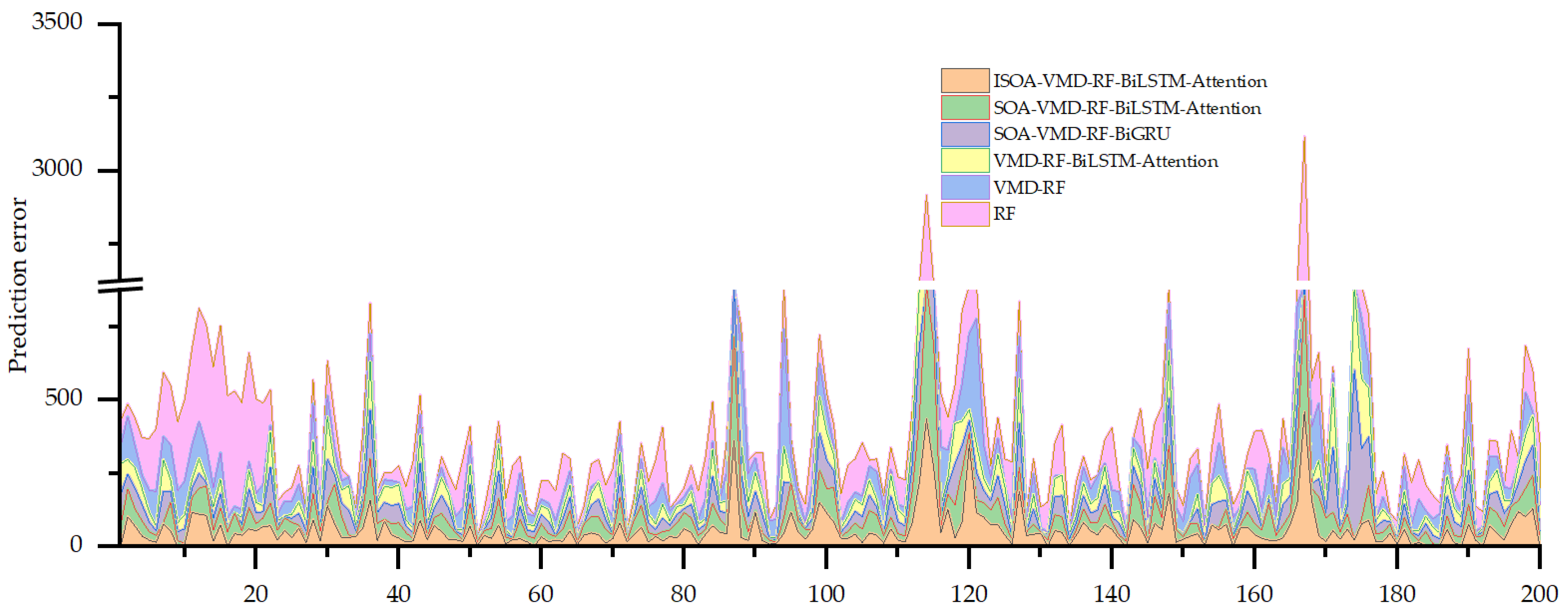
The ISOA–VMD–RF–BiLSTM-attention algorithm outperforms other comparative algorithms in terms of MAE, MAPE, and RMSE for predictions on two industrial building cooling load datasets, while also achieving a higher R². This indicates good prediction accuracy and stability in the field of cooling load prediction.

(2)

The RMSEs of ISO–VMD–RF–BILSTM-attention in two industrial building cooling load data sets were 88.34 and 18.92, compared to 94.99 and 24.77 for SOA–VMD–RF–BiLSTM-attention. Through parameter optimization using the penalty factor for VMD and the number of signal decompositions with envelope entropy as the fitness function, the RMSEs were reduced by approximately 7.1% and 23.6%. This improvement in SOA contributes to enhanced prediction accuracy, especially in complex industrial building scenarios.

Compared with VMD–RF, the RMSE of ISOA–VMD–RF–BiLSTM-attention is 88.34 and 18.92 while VMD–RF has an RMSE of 123.69 and 48.21, resulting in a reduction of approximately 28.5% and 60.8%. This indicates that choosing the appropriate prediction model based on the data spectrum can significantly impact prediction results.

In conclusion, the proposed ISOA–VMD–RF–BiLSTM-attention model excels in optimizing VMD parameters through the ISOA method, employing frequency spectrum for discriminating decomposed IMF components and residuals, predicting high-frequency components with the RF method, forecasting low-frequency components with the BiLSTM-attention method, and finally combining both for accurate predictions. The mechanism behind this approach is to complement each other’s strengths by combining different technologies to handle both short-term fluctuations in the data and capture long-term trends, thus ensuring the accuracy of the prediction while improving the adaptability and robustness of the model to complex non-linear models. This model achieves precise cooling load predictions for industrial buildings while reducing computational complexity.

5.4. Proof of Concept of the Model

In implementing the proposed prediction model on-site, considering its involvement in complex data processing and computation, a hardware platform with sufficient computational capacity is required to ensure efficient data processing and model operation. This not only guarantees the accuracy of predictions but also facilitates real-time or near-real-time forecasting, providing strong technical support for the establishment of energy consumption management systems in industrial buildings. If the site lacks a robust hardware system, a cloud-edge collaboration approach can be adopted, where data collected on-site is sent to the cloud for processing, with the predictive results then delivered back to the on-site platform, thus reducing costs. Overall, through concept verification and comparison of prediction results, the proposed hybrid prediction method not only demonstrates effective forecasting capabilities but also has manageable hardware requirements for practical application, ensuring smooth deployment and execution in real-world settings and showing significant potential for practical use.

6. Conclusions

This research proposes the ISOA–VMD–RF–BiLSTM-attention method to enhance the accuracy of industrial building cooling load prediction. Accurate cooling load prediction can optimize energy utilization, prolong equipment lifespan, reduce carbon emissions, and enhance production efficiency, contributing significantly to sustainability in the industrial sector. The research focuses on a specific industrial building in Hebei, China, collecting its cooling load data. Initially, the ISOA–VMD method decomposes the cooling load data into multiple Intrinsic Mode Function (IMF) components and residuals. Subsequently, the high-frequency IMF components are inputted into the RF model for prediction, while the low-frequency IMF components and residual are inputted into the BiLSTM-attention model for prediction. The final cooling load prediction is obtained by aggregating these predictions. The ISOA method is validated using six test functions, and the proposed method is compared with five benchmark algorithms using four evaluation metrics. The results demonstrate the superiority of the proposed approach. While this study primarily focuses on hourly cooling load prediction, practical applications, especially for HVAC equipment, often require adgvanced planning. Future research will explore further improvements, such as optimizing internal hyperparameters of deep learning methods, to enhance the accuracy of cooling load predictions. This endeavor will not only aim at achieving higher prediction accuracy but also at reinforcing the contributions to sustainability. This includes facilitating the transition towards more energy-efficient and environmentally friendly practices in the industrial sector, thus playing a crucial role in the broader context of sustainable development.

References

1. Zhou, N.; Lin, J. The reality and future scenarios of commercial building energy consumption in China. Energy Build. 2008, 40, 2121–2127. [Google Scholar] [CrossRef]
2. Kong, M.; Dong, B.; Zhang, R.; O’Neill, Z. HVAC energy savings, thermal comfort and air quality for occupant-centric control through a side-by-side experimental study. Appl. Energy 2022, 306, 117987. [Google Scholar] [CrossRef]
3. Zhao, H.; Magoulès, F. A review on the prediction of building energy consumption. Renew. Sustain. Energy Rev. 2012, 16, 3586–3592. [Google Scholar] [CrossRef]
4. Gassar, A.A.A.; Cha, S.H. Energy prediction techniques for large-scale buildings towards a sustainable built environment: A review. Energy Build. 2020, 224, 110238. [Google Scholar] [CrossRef]
5. Liu, Z.; Quan, Z.; Zhao, Y.; Zhang, W.; Yang, M.; Chang, Z. Mass flow rate prediction of a direct-expansion ice thermal storage system using R134a based on dimensionless correlation and artificial neural network. Energy 2024, 391, 130398. [Google Scholar] [CrossRef]
6. Kang, X.; Wang, X.; An, J.; Yan, D. A novel approach of day-ahead cooling load prediction and optimal control for ice-based thermal energy storage (TES) system in commercial buildings. Energy Build. 2022, 275, 112478. [Google Scholar] [CrossRef]
7. Wang, Y.; Hou, J.; Zhou, P.; He, Z.; Wei, S.; You, S.; Zhang, H.; Zheng, X. Performance analysis of ice storage tank with smooth-tube and corrugated-tube heat exchangers based on numerical simulation. Appl. Therm. Eng. 2024, 236, 121591. [Google Scholar] [CrossRef]
8. Griesbach, M.; König-Haagen, A.; Heberle, F.; Brüggemann, D. Multi-criteria assessment and optimization of ice-energy storage systems in combined heat and cold supply networks of a campus building. Energy Convers. Manage 2023, 287, 117118. [Google Scholar] [CrossRef]
9. Mao, Y.; Yu, J.; Zhang, N.; Dong, F.; Wang, M.; Li, X. A hybrid model of commercial building cooling load prediction based on the improved NCHHO-FENN algorithm. J. Build. Eng. 2023, 78, 107660. [Google Scholar] [CrossRef]
10. Huang, Y.; Li, C. Accurate heating, ventilation and air conditioning system load prediction for residential buildings using improved ant colony optimization and wavelet neural network. J. Build. Eng. 2021, 35, 101972. [Google Scholar] [CrossRef]
11. Pandey, B.; Banerjee, R.; Sharma, A. Coupled EnergyPlus and CFD analysis of PCM for thermal management of buildings. Energy Build. 2021, 231, 110598. [Google Scholar] [CrossRef]
12. Cao, J.; Liu, J.; Man, X. A united WRF/TRNSYS method for estimating the heating/cooling load for the thousand-meter scale megatall buildings. Appl. Therm. Eng. 2017, 114, 196–210. [Google Scholar] [CrossRef]
13. Vera-García, F.; Rubio-Rubio, J.J.; López-Belchí, A.; Hontoria, E. Modelling and real-data validation of a logistic centre using TRNSYS®: Influences of the envelope, infiltrations and stored goods. Energy Build. 2022, 275, 112474. [Google Scholar] [CrossRef]
14. Ahamed, M.S.; Guo, H.; Tanino, K. Modeling heating demands in a Chinese-style solar greenhouse using the transient building energy simulation model TRNSYS. J. Build. Eng. 2020, 29, 101114. [Google Scholar] [CrossRef]
15. Mazzeo, D.; Matera, N.; Cornaro, C.; Oliveti, G.; Romagnoni, P.; De Santoli, L. EnergyPlus, IDA ICE and TRNSYS predictive simulation accuracy for building thermal behaviour evaluation by using an experimental campaign in solar test boxes with and without a PCM module. Energy Build. 2020, 212, 109812. [Google Scholar] [CrossRef]
16. Mao, Y.; Yu, J.; Zhang, N.; Zhou, M.; Wang, M. Prediction of thermal comfort indoors and cooling loads based on reasonable zoning using the improved HHO with multi-strategy fusion-FENN algorithm. Build. Environ. 2023, 245, 110944. [Google Scholar] [CrossRef]
17. Cao, W.; Yu, J.; Chao, M.; Wang, J.; Yang, S.; Zhou, M.; Wang, M. Short-term energy consumption prediction method for educational buildings based on model integration. Energy. 2023, 283, 128580. [Google Scholar] [CrossRef]
18. Xie, M.; Qiu, Y.; Liang, Y.; Zhou, Y.; Liu, Z.; Zhang, G. Policies, applications, barriers and future trends of building information modeling technology for building sustainability and informatization in China. Energy Rep. 2022, 8, 7107–7126. [Google Scholar] [CrossRef]
19. Zhang, F.; Chan, A.P.C.; Darko, A.; Chen, Z.; Li, D. Integrated applications of building information modeling and artificial intelligence techniques in the AEC/FM industry. Autom. Constr. 2022, 139, 104289. [Google Scholar] [CrossRef]
20. Lu, C.; Gu, J.; Lu, W. An improved attention-based deep learning approach for robust cooling load prediction: Public building cases under diverse occupancy schedules. Sustain. Cities Soc. 2023, 96, 104679. [Google Scholar] [CrossRef]
21. Abdou, N.; El Mghouchi, Y.; Jraida, K.; Hamdaoui, S.; Hajou, A.; Mouqallid, M. Prediction and optimization of heating and cooling loads for low energy buildings in Morocco: An application of hybrid machine learning methods. J. Build. Eng. 2022, 61, 105332. [Google Scholar] [CrossRef]
22. Emhamed, A.A.; Shrivastava, J. Electrical load distribution forecasting utilizing support vector model (SVM). Mat. Today Proc. 2021, 47, 41–46. [Google Scholar] [CrossRef]
23. Duan, H.; Yin, X.; Kou, H.; Wang, J.; Zeng, K.; Ma, F. Regression prediction of hydrogen enriched compressed natural gas (HCNG) engine performance based on improved particle swarm optimization back propagation neural network method (IMPSO-BPNN). Fuel 2023, 331, 125872. [Google Scholar] [CrossRef]
24. Hu, Y.; Qin, L.; Li, S.; Li, X.; Zhou, R.; Li, Y.; Sheng, W. Adaptive corrected parameters algorithm applied in cooling load prediction based on black-box model: A case study for subway station. Energy Build. 2023, 297, 113429. [Google Scholar] [CrossRef]
25. Lei, L.; Shao, S. Prediction model of the large commercial building cooling loads based on rough set and deep extreme learning machine. J. Build. Eng. 2023, 80, 107958. [Google Scholar] [CrossRef]
26. Song, C.; Yang, H.; Meng, X.B.; Yang, P.; Cai, J.; Bao, H.; Xu, K. A novel deep-learning framework for short-term prediction of cooling load in public buildings. J. Clean. Prod. 2024, 434, 139796. [Google Scholar] [CrossRef]
27. Kavitha, R.J.; Thiagarajan, C.; Priya, P.I.; Anand, A.V.; Al-Ammar, E.A.; Santhamoorthy, M.; Chandramohan, P. Improved Harris Hawks Optimization with Hybrid Deep Learning Based Heating and Cooling Load Prediction on residential buildings. Chemosphere 2022, 309, 136525. [Google Scholar] [CrossRef] [PubMed]
28. Dong, F.; Yu, J.; Quan, W.; Xiang, Y.; Li, X.; Sun, F. Short-term building cooling load prediction model based on DwdAdam-ILSTM algorithm: A case study of a commercial building. Energy Build. 2022, 272, 112337. [Google Scholar] [CrossRef]
29. Yan, X.; Ji, X.; Meng, Q.; Sun, H.; Lei, Y. A hybrid prediction model of improved bidirectional long short-term memory network for cooling load based on PCANet and attention mechanism. Energy 2024, 292, 130388. [Google Scholar] [CrossRef]
30. Guo, J.; Yun, S.; Meng, Y.; He, N.; Ye, D.; Zhao, Z.; Jia, L.; Yang, L. Prediction of heating and cooling loads based on light gradient boosting machine algorithms. Build. Environ. 2023, 236, 110252. [Google Scholar] [CrossRef]
31. Gopila, M.; Suresh, G.; Prasad, D. Random decision forest (RDF) and crystal structure algorithm (CryStAl) for uncertainty consideration of RES & load demands with optimal design of hybrid CCHP systems. Energy 2023, 282, 128545. [Google Scholar]
32. Karijadi, I.; Chou, S.Y. A hybrid RF-LSTM based on CEEMDAN for improving the accuracy of building energy consumption prediction. Energy Build. 2022, 259, 111908. [Google Scholar] [CrossRef]
33. Xu, H.; Liu, Y.; Li, J.; Yu, H.; An, X.; Ma, K.; Liang, Y.; Hu, X.; Zhang, H. Study on the Influence of High and Low Temperature Environment on the Energy Consumption of Battery Electric Vehicles. Energy Rep. 2023, 9, 835–842. [Google Scholar] [CrossRef]
34. Pan, J.; Jing, B.; Jiao, X.; Wang, S. Analysis and application of grey wolf optimizer-long short-term memory. IEEE Access 2020, 8, 121460–121468. [Google Scholar] [CrossRef]
35. Liu, Z.; Yu, J.; Feng, C.; Su, Y.; Dai, J.; Chen, Y. A hybrid forecasting method for cooling load in large public buildings based on improved long short term memory. J. Build. Eng. 2023, 76, 107238. [Google Scholar] [CrossRef]
36. Song, Y.; Xie, H.; Zhu, Z.; Ji, R. Predicting energy consumption of chiller plant using WOA-BiLSTM hybrid prediction model: A case study for a hospital building. Energy Build. 2023, 300, 113642. [Google Scholar] [CrossRef]
37. Hashim, F.A.; Hussien, A.G. Snake Optimizer: A novel meta-heuristic optimization algorithm. Knowl. Based Syst. 2022, 242, 108320. [Google Scholar] [CrossRef]
38. Fang, M.; Zhang, F.; Yang, Y.; Cai, J.; Bao, H.; Xu, K. The influence of optimization algorithm on the signal prediction accuracy of VMD-LSTM for the pumped storage hydropower unit. J. Energy Storage 2024, 78, 110187. [Google Scholar] [CrossRef]
39. Liu, Z.; Liu, H. A novel hybrid model based on GA-VMD, sample entropy reconstruction and BiLSTM for wind speed prediction. Measurement 2023, 222, 113643. [Google Scholar] [CrossRef]
40. Sareen, K.; Panigrahi, B.K.; Shikhola, T.; Chawla, A. A robust De-Noising Autoencoder imputation and VMD algorithm based deep learning technique for short-term wind speed prediction ensuring cyber resilience. Energy 2023, 283, 129080. [Google Scholar] [CrossRef]
41. Yang, B.; Li, M.; Qin, R.; Luo, E.; Duan, J.; Liu, B.; Wang, Y.; Wang, J.; Jiang, L. Extracted power optimization of hybrid wind-wave energy converters array layout via enhanced snake optimizer. Energy 2024, 293, 130529. [Google Scholar] [CrossRef]
42. Yan, C.; Razmjooy, N. Optimal lung cancer detection based on CNN optimized and improved Snake optimization algorithm. Biomed. Signal Process. Control. 2023, 86, 105319. [Google Scholar] [CrossRef]
43. Jiang, Z.; Zhang, Z.; He, X.; Luo, E.; Duan, J.; Liu, B.; Wang, Y.; Wang, J.; Jiang, L. Efficient and accurate TEC modeling and prediction approach with random forest and Bi-LSTM for large-scale region. Adv. Space Res. 2024, 73, 650–662. [Google Scholar] [CrossRef]
44. Zrira, N.; Kamal-Idrissi, A.; Farssi, R.; Khan, H.A. Time series prediction of sea surface temperature based on BiLSTM model with attention mechanism. J. Sea Res. 2024, 198, 102472. [Google Scholar] [CrossRef]
45. Guo, J.; Liu, M.; Luo, P.; Chen, X.; Yu, H.; Wei, X. Attention-based BILSTM for the degradation trend prediction of lithium battery. Energy Rep. 2023, 9, 655–664. [Google Scholar] [CrossRef]
46. Shan, L.; Liu, Y.; Tang, M.; Yang, M. CNN-BiLSTM hybrid neural networks with attention mechanism for well log prediction. J. Pet. Sci. Eng. 2021, 205, 108838. [Google Scholar] [CrossRef]
Figure 1. The schematic illustration of this paper.
Sustainability 16 02522 g001
Figure 2. Comparison between random initialization and sine chaotic mapping initialization graph.
Sustainability 16 02522 g002
Figure 3. The change curve of adaptive inertia weight factor ω .
Sustainability 16 02522 g003
Figure 4. Flow chart for optimizing VMD parameters based on the ISOA.
Sustainability 16 02522 g004
Figure 5. The process flow diagram of the RF algorithm.
Sustainability 16 02522 g005
Figure 6. The signal LSTM cell structure.
Sustainability 16 02522 g006
Figure 7. The BiLSTM network structure.
Sustainability 16 02522 g007
Figure 8. The framework of ISOA-VMD-RF-BiLSTM-Attentiom model.
Sustainability 16 02522 g008
Figure 9. Commercial building hourly cooling load data.
Sustainability 16 02522 g009
Figure 10. Iteration curve of the benchmark function F 1 F 6 .
Sustainability 16 02522 g010
Figure 11. ISOA optimized VMD process.
Sustainability 16 02522 g011
Figure 12. ISOA−VMD cooling load data decomposition results.
Sustainability 16 02522 g012
Figure 13. ISOA−VMD decomposition result spectrum diagram.
Sustainability 16 02522 g013
Figure 14. Comparison of cooling load prediction errors.
Sustainability 16 02522 g014
Figure 15. Comparison of cooling load prediction errors(B).
Sustainability 16 02522 g015