Application of Macro X-ray Fluorescence Fast Mapping to Thickness Estimation of Layered Pigments

Abstract

Even though X-ray fluorescence (XRF) is strictly an atomic method, this technique has been developed mostly at research centers for nuclear physics. One of its most valuable variations is the mapping mode that allows it to shift XRF from a punctual to an image technique. Macro X-ray Fluorescence (MA-XRF) is a widespread analytical technique applied in cultural heritage for characterizing the elemental composition of pigments with a non-destructive, rapid and green approach. When dealing with cultural heritage materials, the sustainability of the applied techniques is directly linked to the limited impact on the work of art. MA-XRF can reveal hidden sub-surface layers or restorations, but, nonetheless, it is hardly adopted for estimating the thickness of layers without resorting to complex Monte Carlo simulations or without combining information from other techniques. Exploiting the recurrent presence of lead white under pictorial layers in historical artworks, we perform a calibration on stand-alone layers produced ad hoc for the relative absorption of Pb L fluorescence lines, and then, their ratio is successfully used to estimate the thickness of azurite and ultramarine blue layers over lead white. The final result is rendered as a heatmap, easy to present to non-technical personnel frequently involved in the cultural heritage field. The new proposed procedure for calculating layer thickness extends the concept of non-invasive applications, paving the way to the possibility of performing stratigraphy without sampling.

1. Introduction

Analyses based on the detection of characteristic X-ray fluorescence are among the most used for application to the study of cultural heritage, encompassing PIXE (particle-induced X-ray emission) [1,2,3], SEM-EDX (scanning electron microscopy–energy-dispersive X-ray spectroscopy) [4,5] and XRF (X-ray fluorescence) [6,7,8,9]. This last acronym expressly refers to the analysis of material obtained through X-ray fluorescence excited by X-rays; this technique, multi-elemental and non-destructive, enables in situ analysis on a high number of measuring points, as no actual sample collection is needed [10,11,12]. This last aspect, in particular, allows us to classify XRF among the green analytical techniques, whose approach within chemistry is to minimize, or even to eliminate, the use of toxic substances used in the pre-treatments of the samples and the generation of waste, indeed employing screening methods for simple on-site investigations, avoiding the processing of a large number of samples [13,14,15]. This is a highly sustainable approach that minimizes the production of hazardous waste with analytical practices that are friendly to the environment. Moreover, the non-invasive approach allows us to perform sustainable analyses on objects as it does not cause any damage or loss of material [16].

Even though XRF (X-ray fluorescence) is strictly an atomic method, this technique has been developed mostly at research centers for nuclear physics [3,17,18,19] and it is considered in several programs of the IAEA (International Agency for Atomic Agency) [20,21]. This is due to both technical and historical reasons; indeed, radioactive sources have been used for a long time as X-ray sources in XRF spectrometers, and the detection stage exploits the same technology as Ion Beam Analyses (IBA) for which XRF is often a complementary spectroscopic technique [22]. One of the variations of XRF is the mapping mode: elemental analysis using MA-XRF spectrometers is non-destructive, rapid and, green, and can reveal hidden sub-surface layers or restorations [23,24,25]. Thus, Macro X-ray Fluorescence [26] is a non-destructive, non-contact analytical technique, widespread in the cultural heritage (CH) domain [27,28], particularly in field activities due to its portability, resulting in hardware being developed both by industrial companies [29] and in-house by research centers [30,31,32,33,34]. Conceptually, MA-XRF shifts elemental analysis from a punctual to an imaging technique [35].

2. Research Aim

The state-of-the-art MA-XRF instrumentation is represented by raster scanning, i.e., mapping acquisition mode, being a time- and space-ordered collection of spectra [36]. MA-XRF is typically adopted for elemental distribution characterization [37,38,39,40,41], and also combined with several other techniques [42,43] and specific data handling [44]. Indeed, even though there are works exploiting X-ray as radiation to perform stratigraphic studies [27,45,46,47,48,49,50,51], MA-XRF has never been devoted to the determination of layer thickness. Indeed, other methods can be used for 3D topography when given conditions are present [52,53,54]. The present work aims at studying the thickness distribution of a pigment layer over a lead white support through XRF mapping. The thickness of a layer is estimated from the ratio of the absorption of the L lines from lead, related to the thickness via the Lambert–Beer law. Lead was chosen due to its wide adoption as a ground layer in artworks and in several pigments [55]. The instrumentation adopted in the present work is the Bruker IRIS, a mobile MA-XRF scanning instrument from Bruker Nano Analytics (Milano, Italy). IRIS is designed to perform in situ analysis in reduced time frames, and this poses a major challenge for the integration time per pixel. Additionally, it must be considered that the results from a stratigraphy may be difficult to present to non-technical staff and to the public; this is a major issue to be considered when working in the CH field. Suitable communication of data for artistic/historical interpretation [56] must be taken into account; indeed, for this reason, we make it possible to present results through a heatmap, an original, more effective and easier-to-interpret way of presenting information to non-skilled final users.

3. Materials and Methods

3.1. Stand-Alone Layers (Standard for Calibration)

The pigments layers (pure pigment in binders; see

Table 1. Stand-alone layers of azurite and binders used for the method calibration.

Backing	Sample Name	Measure 1 [µm]	Measure 2 [µm]	Measure 3 [µm]	Instrument Precision [µm]	Average Thickness [µm]	σ [µm]
OC-FIX17	F4	56	68	57	1	60	7
Acetate	F3	68	109	108	1	95	23
Standard	A	126	128	80	1	111	27
Parafilm	C1	127	136	132	1	132	5
Plastic	C1	156	184	182	1	174	16
OC-FIX (Dis)	B3	210	204	200	1	205	5
OC-FIX (Dis)	B4	296	216	204	1	239	50
OC-FIX	AR1	306	318	329	1	318	12

for the details of thicknesses and binders) used for the calibration of the absorption of X-ray fluorescence were painted by the laboratory of diagnostic for artworks (DIART) of the department of Physics, State University of Milan. The layers were produced around 10 years ago, also inducing some aging effect on the binders; the thicknesses were measured as reported in Section 3.4.

The selected layers are all composed of azurite, an inorganic pigment regularly found in historical paintings, with a blue color [49]. The layers were provided without support and with different binders.

As a base for the layers, a 5 cm thick block of lead was used, to both mechanically support the pigments and, at the same time, provide fluorescence of the lead lines, to simulate a lead white infinite-thickness ground layer. This experimental approach gave us the possibility of using relatively well-defined thicknesses, although it has some limitations as it is a quite rough approximation for pigment layers. Indeed, the Lα and Lβ intensities are affected by the massive thickness of the Pb layer itself as they are subjected to different auto-absorption depending on the finite/infinite thickness of the layer itself, as discussed later in Section 4.3. We note here that no extraction or derivation was performed for the less-than-infinite-thickness substrate as the thickness of the underlying layer is not known in real applications. Indeed, painting layers are intrinsically inhomogeneous and it is not possible to measure the thickness of these underlaying layers with non-destructive techniques. What we propose in the following is to use the output result as the mean value for the thickness.

3.2. Layered Painting Samples (Mockup)

The experimental mockup (Figure 1), used to test the calibration obtained by the samples described in Section 3.1, was created by DIART laboratory about 20 years ago, so it can be considered fully aged for what concerns binder polymerization. In this study, six regions (named A1, A2, A3, B1, B2 and B3; see Figure 1 and description later in this section) containing azurite and ultramarine blue in different layers were analyzed [45]. The support was wood, and the layer structure is described later in this same section. The different horizontal darker strips on each blue layer are due to aging of the applied organic protective varnishes, namely amber-based varnish, no varnish, glossy Dammar and mat Dammar varnish.

For the A1–A3 samples, pigments (azurite on lead white, natural ultramarine—ultramarine blue—on lead white and ultramarine blue over azurite on lead white) are spread in oil over a plaster priming, while for B1–B3 the same pigment combinations are spread in egg tempera; in the following, the results will be presented for the oil layers. The thicknesses obtained in past works from cross sections of the samples [45] are as follows:

• Sample A1: 37 ± 7.4 µm (azurite, upper layer) and 15 ± 7.4 µm (lead white)
• Sample A2: 22 ± 1.5 µm (ultramarine blue, upper layer) and 7.4 ± 7.4 µm (lead white)
• Sample A3: 7.5 ± 1.5 µm (ultramarine blue, upper layer), 18 ± 1.5 µm (azurite, intermediate layer) and 15 ± 7.4 µm (lead white).

3.3. MA-XRF Instrumentation

The Ma-XRF spectrometer used was IRIS, a portable analytical instrument developed by XGLab S.R.L. (Milano, Italy), part of the Bruker Nano Analytics Division [57,58]. It combines two different non-destructive techniques, MA-XRF and Reflectance Spectroscopy (RS), from visible to near-infrared (NIR). RS, not exploited in the present work, can be useful as it can be considered to synergically integrate with XRF data in the case of pictorial multilayers characterized by organic pigments [59,60], but also for glassy materials [61,62]. As for MA-XRF characteristics, the IRIS spectrometer has a maximum scanning speed of 42 mm s⁻¹ and a source–object distance of about 10 mm if the system is properly aligned using the integrated lasers. The integration time per pixel adopted was 60 ms; the X-ray tube was 50 kV and 4 W with a rhodium anode, while the detector was a Silicon Drift Detector (XGLab S.R.L., Milano, Italy) of 50 mm² with a 140 keV spectral resolution at Mn-Kα. The system is remotely controlled via PC, and an integrated CCD camera enables the user to regulate the position in all directions. The device is provided as an integrated solution from the manufacturer (XGLab), comprehensive of tube, detector, lamp and fibers, camera, laser pointers, PC and mechanical components. The available collimators are 0.5 mm, 1 mm, 2 mm in diameter; in the present work, we used the 1 mm collimator. A photoshoot of the measuring setup and its schematic representation are shown in Figure 2.

The motorized frame had dimensions of 40 cm × 60 cm, while the movement along the measuring head axis was 2 cm from the start to the end point.

Data collection was performed using the IRIS control software, which automatically collected, ordered and saved each spectrum into an HDF5 file. Each file was then processed using a python script decompressing the HDF5 file, reading every spectrum (i.e., every pixel’s information individually) and integrating over 3 different ROIs. The first ROI was centered on the lead Mα fluorescence line, and the second and third ROIs were centered, respectively, over the Lα and Lβ lead lines. The extension of the ROIs was chosen as a compromise between the ROIs adopted for the calibration, to collect a proper signal from the higher flux of the infinite-thickness lead sample and to avoid spurious signals with lower flux measurement in actual application. Due to the combination of short measuring times (tens of seconds) and count rates being extremely limited in the peak regions, we did not need to perform any background subtraction; fitting of the peaks was not applied due to the very same reason.

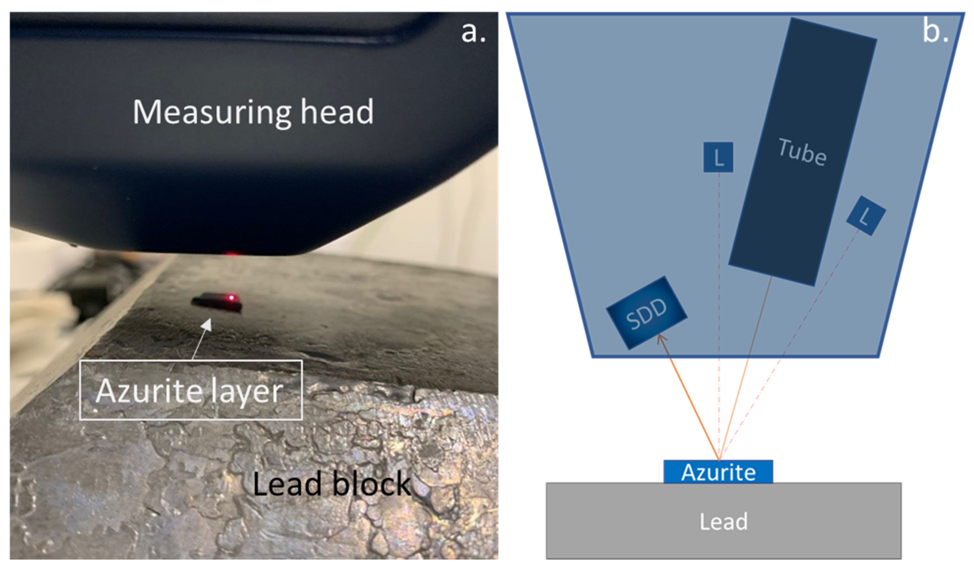
3.4. Feeler for Thickness Measurement of Stand-Alone Layers

The instrumentation exploited to measure the thickness of the stand-alone pigment layers was a feeler gauge with 0.1 µm sensitivity. We measured the thickness at 3 different points and considered the average value and its standard deviation. The feeler measuring area was 1 mm². The uncertainty introduced by the feeler was small compared to variability of the thicknesses themselves, being in the order of tens of microns; thus, the uncertainty was mainly provided by the variability of the thickness itself, according to uncertainty propagation.

4. Results and Discussion

The fluorescence lines used to study the thickness of the pigment layers via their absorption were the ones emitted from lead. In particular, due to the energies of the excitation spectrum, the energy resolution of the detector and the acquisition time per pixel, Mα, Lα and Lβ were selected. The reason for using lead as a reference material is the special role lead white has in paintings, as it was often used as a ground layer [63,64]. This makes it a suitable reference material as source of X-ray fluorescence from the back of layers with unknown thickness. Another primer often used in painting is calcium carbonate (or calcite) [65,66]; this material was not taken into account in this first experimental attempt as the calcium signal is not always visible in XRF spectra, even if the material is present in the lower layers, due to the low energy of its characteristic X-ray emissions.

To compute the calibration curve for the azurite layers from the spectra acquired on stand-alone layers, ROIs over the Lα, Lβ and Mα lead lines were collected and integrated for each pixel. With an integration time of 60 ms, the produced background is typically negligible, as also evident from Figure 3, so no background subtraction was computed. The result from each pixel was then averaged and each layer provided one quadruplet (T, M, La, Lb), where T stands for thickness, and M, La and Lb are the shortening for the absorption edge of the respective lead fluorescence lines. The averaged values were considered for two reasons:

• It is typically of no interest to evaluate the thickness over a specific pixel; instead, it is more interesting to look at the mean layer thickness, thus working with a cluster of pixels.
• Measuring time is too low to obtain reliable results over a specific pigment unless we consider more than one pixel, as real applications usually cannot perform multiple measurements on the same pixel to reach a good counting statistic.

The measurement on the lead reference, that is the support lead block, is also obtained as the average of a mapping acquisition. From these steps, the quantities I₀ for the reference and I_x for the x-th layer are obtained. The ratio of the two quantities is related to the thickness T according to the Lambert–Beer law, Equation (1) [67].

$$\frac{I_x}{I_0}=e^{-\mu T}\triangleq R_x$$

(1)

The law expressed here is derived by modeling the Poisson distribution of absorptions in the case of a mono-elemental, homogeneous and thin medium. To address the multi-element aspect, the equation is modified, adopting an equivalent µ for the mean Z of the layer, assumed invariant for each sample of the same pigment, and for polychromatic beam absorption. In the case of superimposed layers, the effective absorption is the sum of the absorptions from the individual layers. This implies that the derived calibration curve is valid for any pigments showing an equivalent Z equal to or close to the one of the several considered stand-alone layers of azurite spread in oil.

In the following, the ratio R_x is used instead of μ, because the uncertainty propagation will dramatically affect the confidence of the results. Furthermore, since this method can be calibrated to directly relate the ratio to the thickness, the need to find a characteristic curve for the attenuation coefficient can be bypassed. The results are shown in Figure 4, where the dots are the values, the lines the 2-sigma uncertainty on the thickness and the triangles are the 1sigma uncertainty on the mean ratio value.

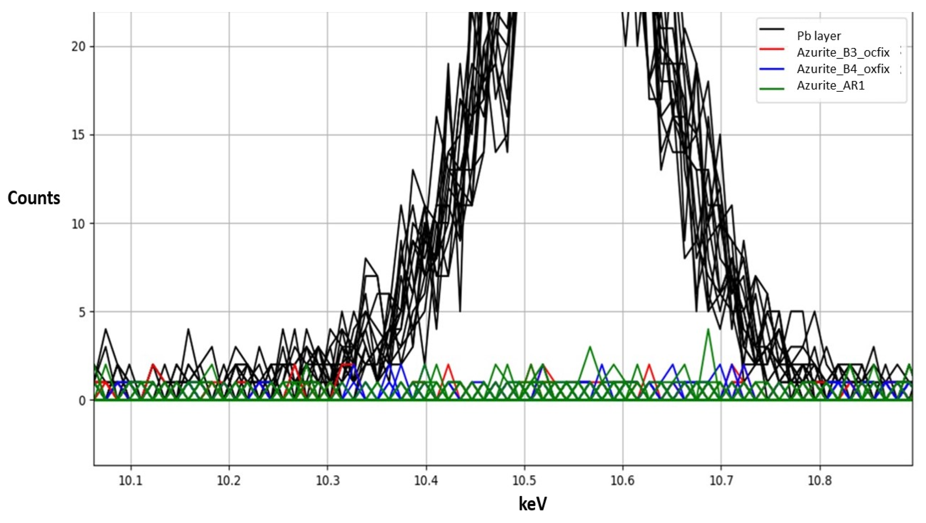
4.1. Thickness–Absorption Relation from Stand-Alone Layers

For higher-thickness layers, the peak intensities are obviously lower due to the greater absorption; in these cases, the statistical noise on the XRF spectra becomes the dominant contribution (Figure 3).

The consequence is that the material becomes opaque, and the ratio is then insensitive to thickness variations. Thus, the ratio is highly unstable and may increase rapidly (Figure 5, top). This always applies to the Mα line, which was thus excluded from the application due to its low energy and inability to provide sensitivity at any of the considered thicknesses (Figure 5, bottom). This could be exploited under suitable conditions, such as with increased flux and measuring time and reduced layer thicknesses. Moreover, the energy region of the Pb Mα line may also present several other lines, and in that case, a simple integral over the spectrum ROI is not enough, and gaussian fitting, or even deconvolution processing, could be required to obtain a proper analysis and meaningful results.

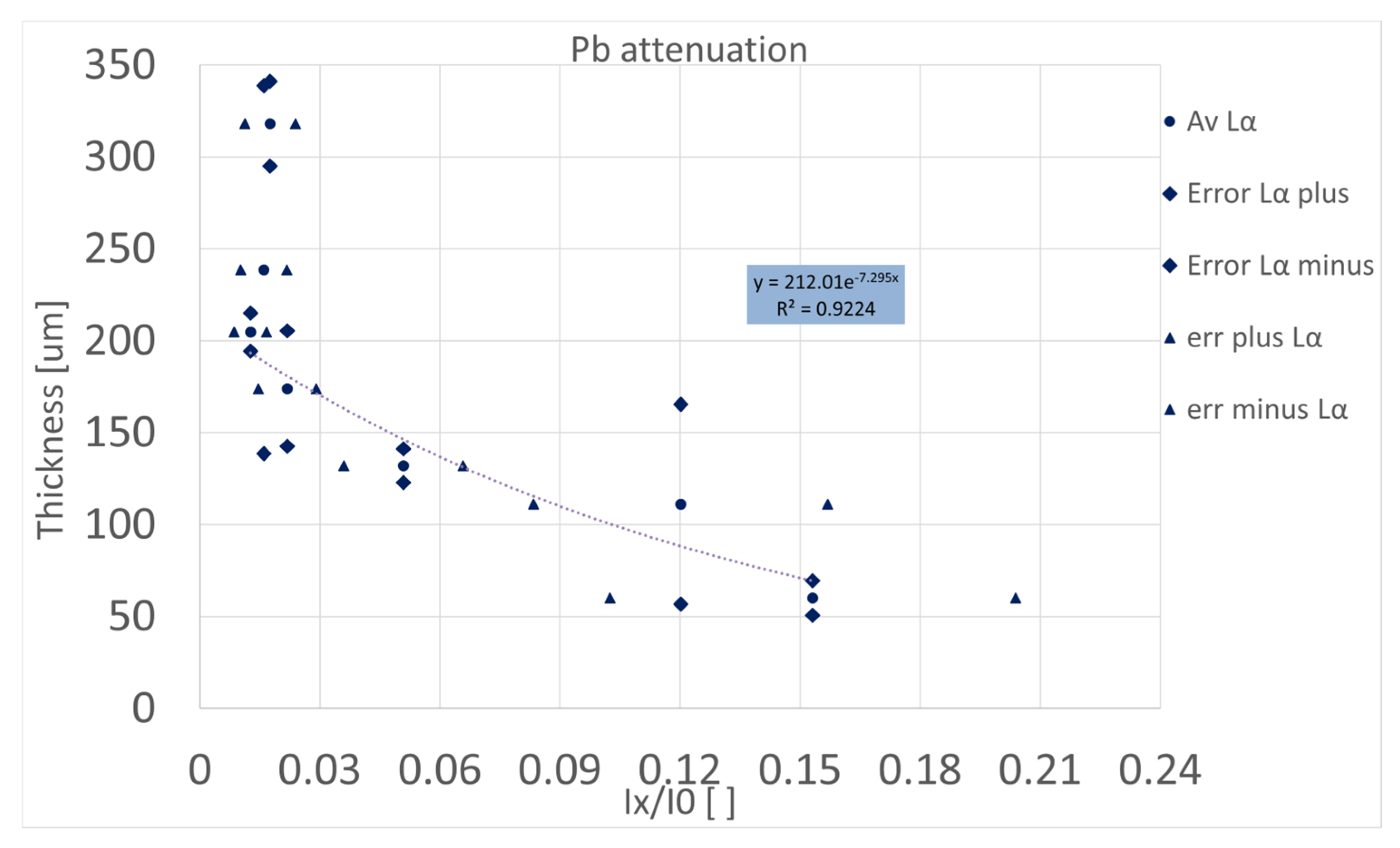
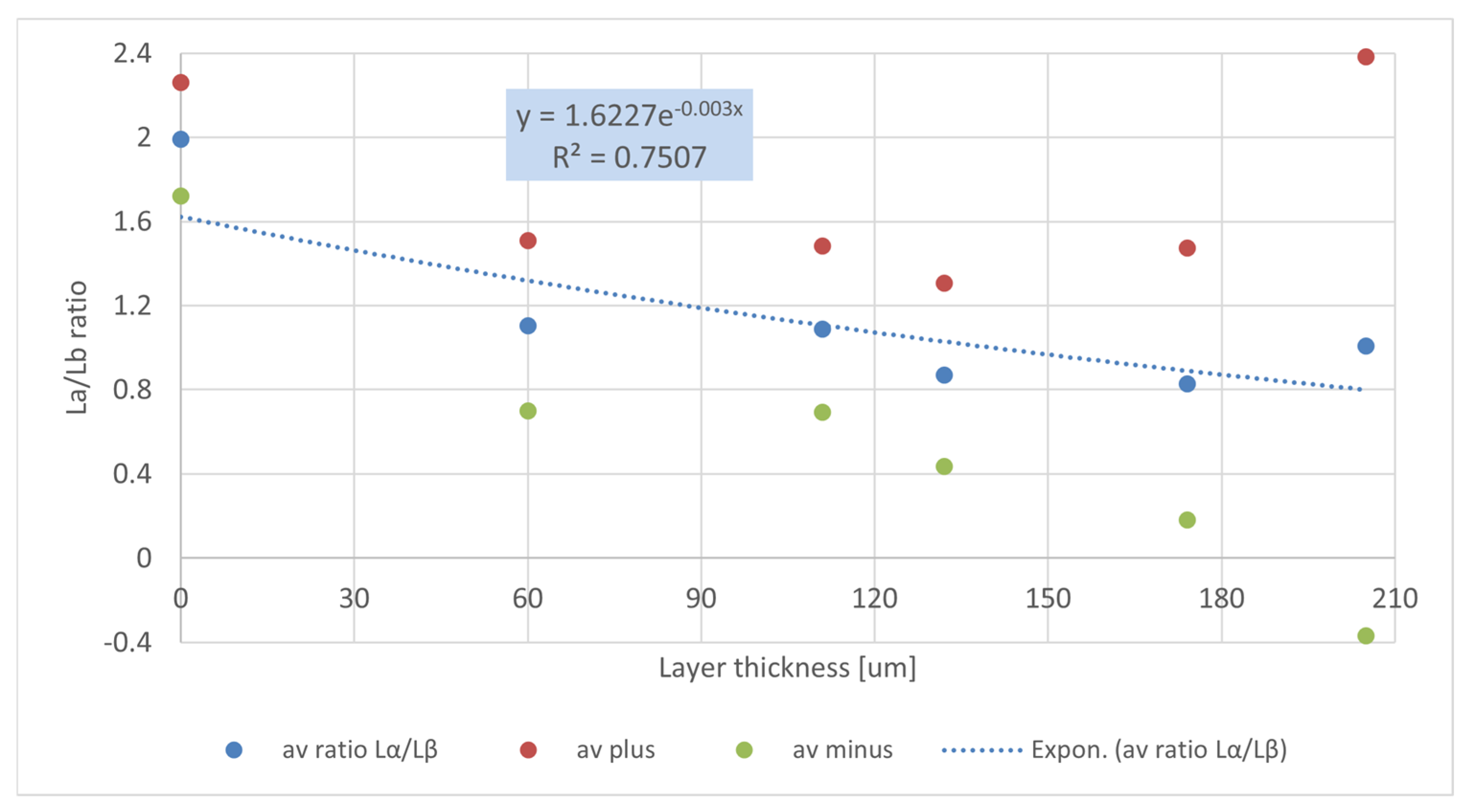
4.2. Calibration Curve

To eliminate the dependence from the intensity of the substrate I₀, it is possible to exploit the ratio of the Lα and the Lβ lines, according to the Lambert–Beer law, for the two different energies of the lines [Equation (2)] [68,69].

$$\frac{L_{\alpha }}{L_{\beta }}=e^{-x\ast [\mu (E_{L\alpha })-\mu (E_{L\beta })]}$$

(2)

As shown in Figure 6, the ratio of the two lines can be as good a predictor as the regression applied to the intensity of a single line over the substrate. For thickness 0, the reported ratio is calculated from the lead substrate signals. Uncertainty on thickness is not reported for the sake of clarity, but it can be found in previous graphics, while for the L line ratio, the green and red points are the two-times expanded uncertainty for the ratio. For the 205 μm thickness, the lower extended uncertainty value is reported to be negative, but obviously, the true value of a thickness cannot be lower than 0. This result means that the intensity lines could be nearly zero and thus affected by a very large error. Please note that R-squared provides an indication of better/worse fitting of a curve compared to other fitting curves under specific assumptions (e.g., single-variable fitting). The obtained value indicates that measurements are affected by high scattering. The functional shape of the curve has not been deduced from our results, but it is based on X-ray absorption laws, and is exponential.

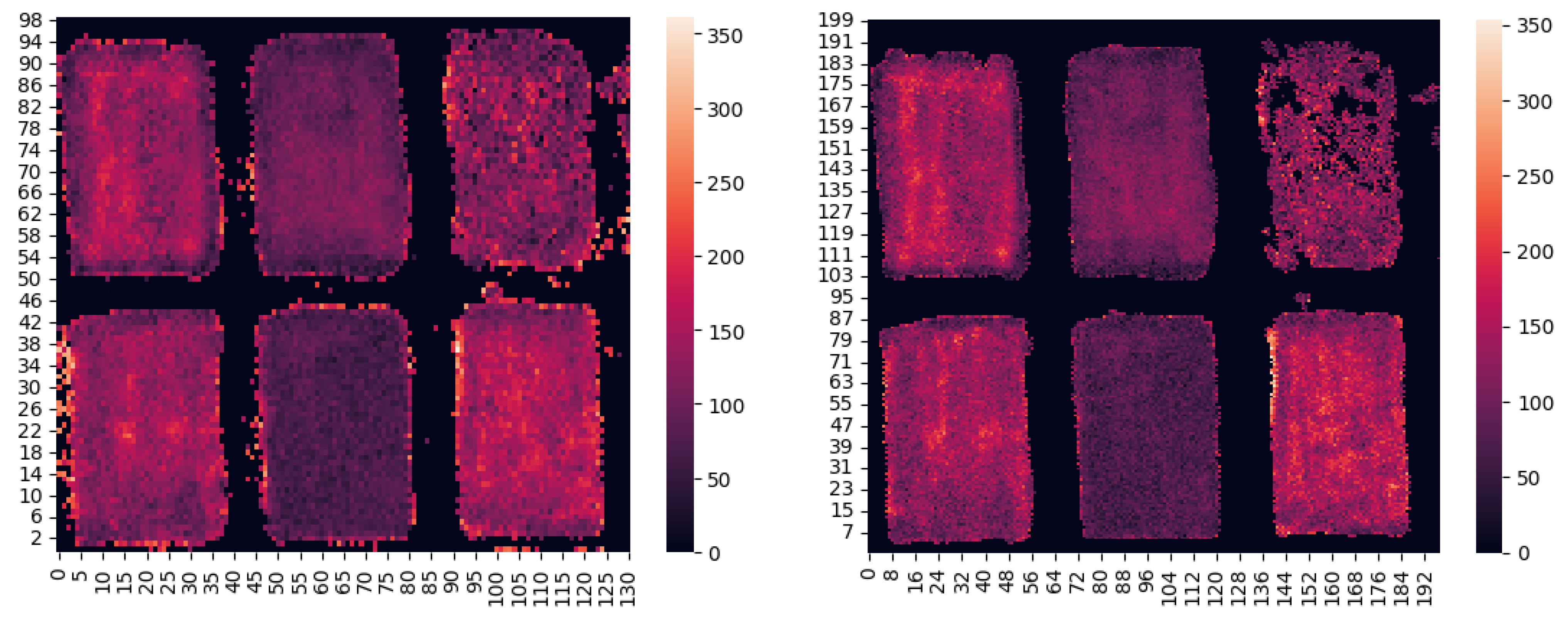
4.3. Thickness Maps of MOCKUP Layers

Computing the ratio of Lα line emission over Lβ line emission for lead can provide an estimate of azurite layer thickness. The energy intervals selected for the two lines were as follows:

10.1 keV ≤ Lα ≤ 10.9 keV    12.2 keV ≤ Lβ ≤ 13 keV

A visual representation of a spectrum with highlighted ROIs is shown in Figure 7, left, with red bars and green bars delimiting, respectively, Lα and Lβ peaks. The spectral peaks obtained from these regions are also shown superimposed in Figure 7, right.

The novelty of the present work lies in the application of the ratio method [69] within a fast scan, that is, when we are dealing with a low count rate for each single spectrum, as is typical in MA-XRF; in this case, even if we expect quite large errors, we demonstrate that the method is highly useful to check the average thickness of pictorial layers. Indeed, the map obtained upon integrating the whole spectrum and the one that originated from integrating around the Lα lead peak are shown in Figure 8, upper row. In both images, especially in the one referring to the whole spectrum, the small holes (about 2 mm²) left from the sampling are evident. This aspect is quite interesting as it allows us, when applied to real cases, to clearly highlight the presence of an eventual lack of painting materials, and thus, to conduct mapping of the conservation state. This approach also allows us to compare MA-XRF with imaging methods [35].

The map in the left part of the middle row in Figure 8 was obtained considering the sulfur Kα (2.3 keV) and Kβ (2.5 keV) lines from gesso primer on the integral of the spectrum between 2.2 keV and 2.6 keV. In this map, the organic finishing layers are also clearly underlined and give a different result depending on their composition and thickness. This allows us to discriminate different surface layers on the same color/part of a painting, and thus, to speculate about the presence of restorations. In this way, MA-XRF proves once again to be competitive against imaging analyses, and can be considered a useful tool each time a surface light element layer must be evaluated, as well as for detecting the presence of patinae in metallic historical objects [70,71,72]. Indeed, considering emissions at such low energies, and thanks to the high performance of the IRIS X-ray detector, it is even able to highlight dark stains in mockups with oil as a binder due to oil spreading in the primer.

From the ROIs reported in Figure 7, the integrals were computed, and then, from the ratio of the integrals of the two emission lines, the thickness was calculated with the inverted formula obtained from the calibration procedure, shown in Equation (3). The output is represented, as in the right part of the middle row in Figure 8, via heatmap plotting. The plot was created using the Python open-source library Seaborn.

$$T=-\frac{1}{0.003}\ln \frac{\raisebox{1ex}{${\sum }_{E=10.1 keV}^{10.9 keV}I\left(E\right)$}\!\left/ \!\raisebox{-1ex}{${\sum }_{E=12.2 keV}^{13 keV}I\left(E\right)$}\right.}{1.6227}$$

(3)

We would like to stress that the aim of this study is to provide a tool for presenting an average estimation of the thickness of a layer to non-technical users. The discussion of uncertainties on the experimental coefficients of the calibration and their propagation is beyond the aim of our work, since the aim is not to provide a precise estimation of the layer thickness (a pixel is not representative of an inhomogeneous layer), but rather, to create a representation tool. The aim is neither to provide a metrological reference for the thickness measurement nor to validate a theoretical curve.

The resulting map showed two issues:

• The obtained image was transposed with respect to the actual object;
• The support is represented as a mid-thickness layer, which is incorrect.

The solutions we adopted are the following:

• The information from the image was stored using the Python Pandas open-source library, exploiting the DataFrame built-in object. DataFrames are created as tables that collect keys in the form of [row][column]. On the contrary, the IRIS software creates a matrix of the type [column][row][spectrum], and populates it starting from the bottom left, scanning towards the right and ending at the top right. Therefore, it is necessary to lock the columns and range on the rows.
• Since the wood support presents noise in the lead line regions, due to backscattered radiation from the excitation source, the contrast can be highly increased considering a threshold to be overcome by at least one of the ROIs’ integrals. That threshold was set as the number of bins in the ROI times a constant of 1.1.

The output from the fast acquisition and from the high-spatial-resolution acquisition obtained after these implementations are shown, respectively, in the lower row of Figure 8. The parameters of the acquisitions are described in

Table 2. Acquisitions parameters.

	Fast Scanning	High-Resolution Scanning
Time [s]	389.1	1188.0 s
Number of pixels	99 × 132	200 × 199
Pixel dimensions [mm × mm]	2 × 1.512	1 × 1
Collimator diameter [mm]	2	1
Integration time [ms/pixel]	30	30
Current [mA]	100	200
Tension [kV]	50	50
Filtering, anode materials	No filter, Rh	No filter, Rh

.

Applying Equation (3), an estimation of the local thickness is provided. Every pixel providing a ratio over 1.7 was set to 0 thickness, representing the value from lead direct fluorescence.

From both the fast-scanning and high-resolution acquisitions, the thickness map was thus successfully obtained. It is worth recalling that fast and high-resolution scans are performed with different integration times and collimator diameters. Due to inhomogeneity of the substrate, the difference in collimator diameters may affect the output result of the thickness estimation, since the averaging effect of a smaller collimator is reduced compared to a larger one, producing different results, as evident in Figure 8.

The mean estimated thicknesses of azurite of the three samples spread in oils (A1, A2 and A3 in Figure 1) are, respectively, A1 = 93 ± 59 µm, A2 = 63 ± 63 µm and A3 = 96 ± 58 µm. The expected thickness for azurite layers, reported in Section 3.2, are 37 ± 7.4 µm for A1, no azurite layer for A2, and 18 ± 1.5 µm for A3. For the A1 layer, the thickness estimation is coherent, inside the error, with the one measured from the cross section. For A2, a layer made of ultramarine blue alone (no azurite present, so no Cu signal besides the background), the result is negligible, and this indicates the absence of the investigated pigments and the Cu signal to be below the detection limit of the spectrometer. Moreover, in cases whereby a Cu signal is present from impurities of the materials layered, the calibration obtained in this work would obviously not be useful for calculating the lapis lazuli layer thickness. For the A3 layer, the obtained average thickness is highly overestimated and not in good agreement with measured one. In this peculiar case, the azurite layer is not the upper layer, but it is covered by an ultramarine blue layer. Considering the chemical composition of lapis lazuli [73], which can be written as (Na,Ca)₈(SO₄,S,Cl)₂(AlSiO₄)₆, and also considering the dilution in linseed oil, which can be considered to be linoleic acid [45], the variation in the absorption coefficient, respectively, for the Lα and Lβ Pb lines does not significantly affect the ratio. Once again, we cannot use the obtained calibration for calculating the thickness of the lapis lazuli layer.

A fundamental aspect to be taken into account is that, as already indicated in Section 3.1, underlying lead white layers in paintings do not have infinite thickness [74]; in extreme cases, the lead-based preparatory layer can be so thin that no signal from lead would pass the azurite layer, even if it is a rare situation. It is worth noting that the overestimation of the layer thickness is due, in part, to the strong hypothesis made when performing the calibration: the lead support must be sufficiently thick to be approximated as infinite for X-ray penetration compared to the pigment layer thickness. That is, the actual lead white layer could produce fewer L signals. It has been demonstrated [68] that the value for Au (La/Lb), due to self-attenuation, does not change in an appreciable manner with thickness, reaching an almost constant value for a thickness of about 20 μm, implying that the results for the A1 layers are less affected by this aspect. As shown from the invasive analysis results [45], the lead white layer is typically thinner than the blue layer, so the fluorescence from the lead cannot build up completely, resulting in Lβ line underestimation and subsequent thickness overestimation. This effect can be effectively mitigated by calibrating the instrument on lead white pigment layers instead of a thick block of metallic lead. For metals, it has been demonstrated that when the incident radiation is sufficiently higher than the absorption edge, the ratio in the case of infinite thick and thin samples can be calculated as the ratio of the linear attenuation coefficient (in cm⁻¹) at the energy of its Lα with that one at the energy of its Lβ [69]. This could suggest a correction factor to use for refining of our method.

A further aspect to be taken into account to explain the difference from the measured thickness of the A3 sample is the percentage of binder in the pictorial layers, which may vary with the different adsorption properties of the pigments themselves, i.e., azurite and lapis lazuli may require different oil concentrations to be conveniently applied. In this regard, the results obtained in the already quoted work [45] on the same mockups also show an overestimation of the azurite layer when it is supposed to be in a mixture with 90% binder, which is the case for our stand-alone calibration samples.

We must thus keep in mind that this kind of calculation must forcibly be considered for estimations, as it is also an estimation of the measured average value over a hand-layered pigment; in fact, the pigment layers spread out by a brush by the artist’s hand, as in our case, makes the layers not constant in thickness. Indeed, the non-uniform layers are highlighted in the reported thickness maps and are also evident from the large errors reported in the thickness determination obtained by cross-section measurements [45].

Moreover, in real cases, lead can be present in pigment layers, as white lead in mixtures, or as lead-based pigment, such as lead-based yellows or reds; in these situations, this method is obviously not applicable.

5. Conclusions

When dealing with analyses of art objects, sustainability must be intended regarding the possibility of performing material characterization with virtually no impact on the object itself. In the present paper, MA-XRF—a strictly non-invasive technique—is exploited to evaluate pigment layer thickness. The measuring of several azurite layers of increasing thicknesses allowed us to effectively produce a calibration curve, which mapped the ratio of the intensities of the transmitted fluorescence of Lα and Lβ lines on a lead-based supporting block through the layers to the thickness of these layers. After the calibration curve was obtained, the method was tested on a group of layers of azurite and ultramarine blue with the thicknesses of the whole structure measured. The resulting heatmaps can be useful in presenting the results and obtaining an estimate of the thickness of the pigment depositions.

Thickness maps are an effective tool both for conducting a more accurate analysis of the pigments on a painting and as preliminary screening to identify areas for an invasive analysis. The obtained results demonstrate that typical scanning times are sufficient to apply this method. The methodology can be applied using a unique calibration curve in the case of pigments with a mean Z equivalent, simplifying the calibration procedure. Furthermore, heatmaps are easier to present both to the public and to non-scientific staff, helping in results communication and project validation.

The present research can be extended in terms of both the analytical techniques employed and in terms of pigments and testing, and finally, in terms of data analysis. The X-ray technique can be complemented by other techniques, such as Reflectance Spectroscopy [75,76,77,78], or X-ray Diffraction [79,80,81], also using its Synchrotron-based version [82,83], or other techniques [84,85,86], like Optical Coherence Tomography (OCT) [87,88] and Terahertz Tomography [89,90,91]. This approach would give two main benefits: better characterizing multi-layer thicknesses and accounting for pigment dilution.

In terms of pigments, there are a huge number of pigments that can be measured to obtain specific calibration curves, and also the effects introduced by the superposition of layers.

Finally, the data analytics procedure can be improved by introducing image processing to further increase the contrast and enhance the edges. The source of the high uncertainty achieved is related mainly to a lack of uniformity over the pigment layers, adequate for human handwork processes over dimensions in the order of tens of microns, and to short measuring time; recall that the time per pixel employed was 0.03 s. Finally, it is important to consider that in such an application the objective is to obtain an estimate of the order of magnitude of the thickness of a sample, such as tens or hundreds of microns.

The maps show that the simple correlation from the Lambert–Beer law can provide meaningful results and can be applied to portable X-ray instrumentation once the calibration curves are provided.

We can therefore observe another interesting result from the Bruker IRIS MA-XRF scanner, which is the possibility to detect the different varnish layers from the absorption on Sulfur K lines and to clearly show the conservation state of an investigated painting.

This non-invasive approach paves the way to the fully sustainable evaluation of layer thickness, avoiding sampling and thus the use of toxic substances and the generation of waste. XRF proved once again to allow fast and simple on-site investigations without the necessity of processing a large number of samples, thus going in the direction of the sustainable and responsible preservation and management of cultural heritage materials.

References

1. Vadrucci, M.; Bazzano, G.; Borgognoni, F.; Chiari, M.; Mazzinghi, A.; Picardi, L.; Ronsivalle, C.; Ruberto, C.; Taccetti, F. A New Small-Footprint External-Beam PIXE Facility for Cultural Heritage Applications Using Pulsed Proton Beams. Nucl. Instrum. Methods Phys. Res. Sect. B Beam Interact. Mater. At. 2017, 406, 314–317. [Google Scholar] [CrossRef]
2. Calligaro, T. PIXE in the Study of Archaeological and Historical Glass. X-ray Spectrom. 2008, 37, 169–177. [Google Scholar] [CrossRef]
3. Sottili, L.; Giuntini, L.; Mazzinghi, A.; Massi, M.; Carraresi, L.; Castelli, L.; Czelusniak, C.; Giambi, F.; Mandò, P.A.; Manetti, M.; et al. The Role of PIXE and XRF in Heritage Science: The INFN-CHNet LABEC Experience. Appl. Sci. 2022, 12, 6585. [Google Scholar] [CrossRef]
4. Moropoulou, A.; Zendri, E.; Ortiz, P.; Delegou, E.T.; Ntoutsi, I.; Balliana, E.; Becerra, J.; Ortiz, R. Scanning Microscopy Techniques as an Assessment Tool of Materials and Interventions for the Protection of Built Cultural Heritage. Scanning 2019, 2019, e5376214. [Google Scholar] [CrossRef]
5. Calia, A.; Lettieri, M.; Quarta, G. Cultural Heritage Study: Microdestructive Techniques for Detection of Clay Minerals on the Surface of Historic Buildings. Appl. Clay Sci. 2011, 53, 525–531. [Google Scholar] [CrossRef]
6. Ruvalcaba Sil, J.L.; Ramírez Miranda, D.; Aguilar Melo, V.; Picazo, F. SANDRA: A Portable XRF System for the Study of Mexican Cultural Heritage. X-ray Spectrom. 2010, 39, 338–345. [Google Scholar] [CrossRef]
7. Liritzis, I.; Zacharias, N. Portable XRF of Archaeological Artifacts: Current Research, Potentials and Limitations. In X-ray Fluorescence Spectrometry (XRF) in Geoarchaeology; Shackley, M.S., Ed.; Springer: New York, NY, USA, 2011; pp. 109–142. ISBN 978-1-4419-6886-9. [Google Scholar]
8. Andrić, V.; Gajić-Kvaščev, M.; Crkvenjakov, D.K.; Marić-Stojanović, M.; Gadžurić, S. Evaluation of Pattern Recognition Techniques for the Attribution of Cultural Heritage Objects Based on the Qualitative XRF Data. Microchem. J. 2021, 167, 106267. [Google Scholar] [CrossRef]
9. Vaggelli, G.; Cossio, R. μ-XRF Analysis of Glasses: A Non-Destructive Utility for Cultural Heritage Applications. Analyst 2012, 137, 662–667. [Google Scholar] [CrossRef]
10. Mantler, M.; Schreiner, M. X-ray Fluorescence Spectrometry in Art and Archaeology. X-ray Spectrom. 2000, 29, 3–17. [Google Scholar] [CrossRef]
11. Dran, J.C.; Calligaro, T.; Salomon, J. Particle Induced X-ray Emission. In Modern Analytical Methods in Art and Arhaeology; Ciliberto, E., Spoto, G., Eds.; John Wiley & Sons: Hoboken, NJ, USA, 2000; Volume 155, pp. 135–166. [Google Scholar]
12. José-Yacaman, M.; Ascensio, J.A. Electron Microscopy and Ots Application to the Study of Archaeological Materials and Art Preservation. In Modern Analytical Methods in Art and Archaeology; Ciliberto, E., Spoto, G., Eds.; John Wiley & Sons: Hoboken, NJ, USA, 2000; Volume 155, pp. 405–444. [Google Scholar]
13. Bilo, F.; Cirelli, P.; Borgese, L. Elemental Analysis of Particulate Matter by X-ray Fluorescence Methods: A Green Approach to Air Quality Monitoring. TrAC Trends Anal. Chem. 2024, 170, 117427. [Google Scholar] [CrossRef]
14. Chojnacka, K.; Mikulewicz, M. Green Analytical Methods of Metals Determination in Biosorption Studies. TrAC Trends Anal. Chem. 2019, 116, 254–265. [Google Scholar] [CrossRef]
15. He, Y.; Tang, L.; Wu, X.; Hou, X.; Lee, Y. Spectroscopy: The Best Way Toward Green Analytical Chemistry? Appl. Spectrosc. Rev. 2007, 42, 119–138. [Google Scholar] [CrossRef]
16. Balliana, E.; Ricci, G.; Pesce, C.; Zendri, E. Assessing the Value of Green Conservation for Cultural Heritage: Positive and Critical Aspects of Already Available Methodologies. Int. J. Conserv. Sci. 2016, 7, 185–202. [Google Scholar]
17. Kučera, J.; Kameník, J.; Havránek, V.; Krausová, I.; Světlík, I.; Pachnerová Brabcová, K.; Fikrle, M.; Chvátil, D. Recent Achievements in NAA, PAA, XRF, IBA and AMS Applications for Cultural Heritage Investigations at Nuclear Physics Institute, Řež. Physics 2022, 4, 491–503. [Google Scholar] [CrossRef]
18. NCSR “Demokritos” Institute of Nuclear and Particle Physics. Available online: http://www.inp.demokritos.gr/xrf/portable-xrf/ (accessed on 12 February 2024).
19. Sri Lanka Atomic Energy Board. X-ray Fluorescence (XRF) Laboratory. Available online: https://aeb.gov.lk/x-ray-fluorescence-xrf-laboratory/ (accessed on 12 February 2024).
20. International Atomic Energy Agency (IAEA). XRF-Training Program. Available online: https://nucleus.iaea.org/sites/nuclear-instrumentation/Pages/XRF-Training.aspx#:~:text=The%20training%20programs%20on%20XRF,from%208%20to%2014%20weeks.&text=Introduction%20to%20Quantitative%20analysis%3A%20Fundamentals,of%20possible%20approaches%20for%20quantification (accessed on 12 February 2024).
21. IAEA. Final Report of a Coordinated Research Project 2000–2003: In Situ Applications of X-ray Fluorescence Techniques. Available online: https://www-pub.iaea.org/MTCD/Publications/PDF/te_1456_web.pdf (accessed on 12 February 2024).
22. Macková, A.; MacGregor, D.; Azaiez, F.; Nyberg, J.; Piasetzky, E. Nuclear Physics for Cultural Heritage; Nuclear Physics Division of the European Physical Society: Mulhouse, France, 2016. [Google Scholar]
23. Scruggs, B.; Haschke, M.; Herczeg, L.; Nicolosi, J. XRF Mapping: New Tools for Distribution Analysis. Adv. X-ray Anal. 2000, 42, 19–25. [Google Scholar]
24. Campos, P.H.O.V.; Appoloni, C.R.; Rizzutto, M.A.; Leite, A.R.; Assis, R.F.; Santos, H.C.; Silva, T.F.; Rodrigues, C.L.; Tabacniks, M.H.; Added, N. A Low-Cost Portable System for Elemental Mapping by XRF Aiming In Situ Analyses. Appl. Radiat. Isot. 2019, 152, 78–85. [Google Scholar] [CrossRef]
25. Haschke, M.; Rossek, U.; Tagle, R.; Waldschläger, U. Fast elemental mapping with micro-XRF. Adv X-ray Anal. 2012, 55, 286–298. [Google Scholar]
26. Alfeld, M. MA-XRF for Historical Paintings: State of the Art and Perspective. Microsc. Microanal. 2020, 26, 72–75. [Google Scholar] [CrossRef]
27. Galli, A.; Caccia, M.; Alberti, R.; Bonizzoni, L.; Aresi, N.; Frizzi, T.; Bombelli, L.; Gironda, M.; Martini, M. Discovering the Material Palette of the Artist: A p-XRF Stratigraphic Study of the Giotto Panel ‘God the Father with Angels’. X-ray Spectrom. 2017, 46, 435–441. [Google Scholar] [CrossRef]
28. Gu, B.; Mishra, B.; Miller, C.; Wang, W.; Lai, B.; Brooks, S.C.; Kemner, K.M.; Liang, L. X-ray Fluorescence Mapping of Mercury on Suspended Mineral Particles and Diatoms in a Contaminated Freshwater System. Biogeosciences 2014, 11, 5259–5267. [Google Scholar] [CrossRef]
29. Alberti, R.; Frizzi, T.; Bombelli, L.; Gironda, M.; Aresi, N.; Rosi, F.; Miliani, C.; Tranquilli, G.; Talarico, F.; Cartechini, L. CRONO: A Fast and Reconfigurable Macro X-ray Fluorescence Scanner for in-Situ Investigations of Polychrome Surfaces. X-ray Spectrom. 2017, 46, 297–302. [Google Scholar] [CrossRef]
30. Pouyet, E.; Barbi, N.; Chopp, H.; Healy, O.; Katsaggelos, A.; Moak, S.; Mott, R.; Vermeulen, M.; Walton, M. Development of a Highly Mobile and Versatile Large MA-XRF Scanner for in Situ Analyses of Painted Work of Arts. X-ray Spectrom. 2021, 50, 263–271. [Google Scholar] [CrossRef]
31. Mazzinghi, A.; Ruberto, C.; Castelli, L.; Ricciardi, P.; Czelusniak, C.; Giuntini, L.; Mandò, P.A.; Manetti, M.; Palla, L.; Taccetti, F. The Importance of Being Little: MA-XRF on Manuscripts on a Venetian Island. X-ray Spectrom. 2021, 50, 272–278. [Google Scholar] [CrossRef]
32. Ruberto, C.; Mazzinghi, A.; Massi, M.; Castelli, L.; Czelusniak, C.; Palla, L.; Gelli, N.; Betuzzi, M.; Impallaria, A.; Brancaccio, R.; et al. Imaging Study of Raffaello’s “La Muta” by a Portable XRF Spectrometer. Microchem. J. 2016, 126, 63–69. [Google Scholar] [CrossRef]
33. Taccetti, F.; Castelli, L.; Czelusniak, C.; Gelli, N.; Mazzinghi, A.; Palla, L.; Ruberto, C.; Censori, C.; Lo Giudice, A.; Re, A.; et al. A Multipurpose X-ray Fluorescence Scanner Developed for in Situ Analysis. Rend. Fis. Acc. Lincei 2019, 30, 307–322. [Google Scholar] [CrossRef]
34. Lins, S.A.B.; Manso, M.; Lins, P.A.B.; Brunetti, A.; Sodo, A.; Gigante, G.E.; Fabbri, A.; Branchini, P.; Tortora, L.; Ridolfi, S. Modular MA-XRF Scanner Development in the Multi-Analytical Characterisation of a 17th Century Azulejo from Portugal. Sensors 2021, 21, 1913. [Google Scholar] [CrossRef] [PubMed]
35. Orsilli, J.; Galli, A.; Bonizzoni, L.; Caccia, M. More than XRF Mapping: STEAM (Statistically Tailored Elemental Angle Mapper) a Pioneering Analysis Protocol for Pigment Studies. Appl. Sci. 2021, 11, 1446. [Google Scholar] [CrossRef]
36. Vanhoof, C.; Bacon, J.R.; Fittschen, U.E.A.; Vincze, L. Atomic Spectrometry Update—A Review of Advances in X-ray Fluorescence Spectrometry and Its Special Applications. J. Anal. At. Spectrom. 2021, 36, 1797–1812. [Google Scholar] [CrossRef]
37. Dos Santos, H.C.; Caliri, C.; Pappalardo, L.; Catalano, R.; Orlando, A.; Rizzo, F.; Romano, F.P. Real-Time MA-XRF Imaging Spectroscopy of the Virgin with the Child Painted by Antonello de Saliba in 1497. Microchem. J. 2018, 140, 96–104. [Google Scholar] [CrossRef]
38. Romano, F.P.; Caliri, C.; Nicotra, P.; Martino, S.D.; Pappalardo, L.; Rizzo, F.; Santos, H.C. Real-Time Elemental Imaging of Large Dimension Paintings with a Novel Mobile Macro X-ray Fluorescence (MA-XRF) Scanning Technique. J. Anal. At. Spectrom. 2017, 32, 773–781. [Google Scholar] [CrossRef]
39. Sciutto, G.; Frizzi, T.; Catelli, E.; Aresi, N.; Prati, S.; Alberti, R.; Mazzeo, R. From Macro to Micro: An Advanced Macro X-ray Fluorescence (MA-XRF) Imaging Approach for the Study of Painted Surfaces. Microchem. J. 2018, 137, 277–284. [Google Scholar] [CrossRef]
40. Saverwyns, S.; Currie, C.; Lamas-Delgado, E. Macro X-ray Fluorescence Scanning (MA-XRF) as Tool in the Authentication of Paintings. Microchem. J. 2018, 137, 139–147. [Google Scholar] [CrossRef]
41. Ricciardi, P.; Legrand, S.; Bertolotti, G.; Janssens, K. Macro X-ray Fluorescence (MA-XRF) Scanning of Illuminated Manuscript Fragments: Potentialities and Challenges. Microchem. J. 2016, 124, 785–791. [Google Scholar] [CrossRef]
42. Cavaleri, T.; Pelosi, C.; Ricci, M.; Laureti, S.; Romano, F.P.; Caliri, C.; Ventura, B.; De Blasi, S.; Gargano, M. IR Reflectography, Pulse-Compression Thermography, MA-XRF, and Radiography: A Full-Thickness Study of a 16th-Century Panel Painting Copy of Raphael. J. Imaging 2022, 8, 150. [Google Scholar] [CrossRef]
43. Bicchieri, M.; Biocca, P.; Caliri, C.; Romano, F.P. Complementary MA-XRF and μ-Raman Results on Two Leonardo Da Vinci Drawings. X-ray Spectrom. 2021, 50, 401–409. [Google Scholar] [CrossRef]
44. Kogou, S.; Lee, L.; Shahtahmassebi, G.; Liang, H. A New Approach to the Interpretation of XRF Spectral Imaging Data Using Neural Networks. X-ray Spectrom. 2021, 50, 310–319. [Google Scholar] [CrossRef]
45. Bonizzoni, L.; Galli, A.; Poldi, G.; Milazzo, M. In Situ Non-Invasive EDXRF Analysis to Reconstruct Stratigraphy and Thickness of Renaissance Pictorial Multilayers. X-ray Spectrom. 2007, 36, 55–61. [Google Scholar] [CrossRef]
46. Trojek, T.; Wegrzynek, D. X-ray Fluorescence Kα/Kβ Ratios for a Layered Specimen: Comparison of Measurements and Monte Carlo Calculations with the MCNPX Code. Nucl. Instrum. Methods Phys. Res. Sect. A Accel. Spectrometers Detect. Assoc. Equip. 2010, 619, 311–315. [Google Scholar] [CrossRef]
47. Fiorini, C.; Gianoncelli, A.; Longoni, A.; Zaraga, F. Determination of the Thickness of Coatings by Means of a New XRF Spectrometer. X-ray Spectrom. 2002, 31, 92–99. [Google Scholar] [CrossRef]
48. Vavrik, D.; Kytyr, D.; Zemlicka, J. Stratigraphy of a Layered Structure Utilizing XRF and Scattered Photons. J. Inst. 2020, 15, C03011. [Google Scholar] [CrossRef]
49. Bonizzoni, L.; Colombo, C.; Ferrati, S.; Gargano, M.; Greco, M.; Ludwig, N.; Realini, M. A Critical Analysis of the Application of EDXRF Spectrometry on Complex Stratigraphies. X-ray Spectrom. 2011, 40, 247–253. [Google Scholar] [CrossRef]
50. Orsilli, J.; Migliori, A.; Padilla-Alvarez, R.; Martini, M.; Galli, A. AR-XRF Measurements and Data Treatment for the Evaluation of Gilding Samples of Cultural Heritage. J. Anal. At. Spectrom. 2023, 38, 174–185. [Google Scholar] [CrossRef]
51. Orsilli, J.; Martini, M.; Galli, A. Angle Resolved-XRF Analysis of Puebla Ceramic Decorations. Spectrochim. Acta Part B At. Spectrosc. 2023, 210, 106809. [Google Scholar] [CrossRef]
52. Liang, H.; Lucian, A.; Lange, R.; Cheung, C.S.; Su, B. Remote Spectral Imaging with Simultaneous Extraction of 3D Topography for Historical Wall Paintings. ISPRS J. Photogramm. Remote Sens. 2014, 95, 13–22. [Google Scholar] [CrossRef]
53. Förste, F.; Bauer, L.; Heimler, K.; Hansel, B.; Vogt, C.; Kanngießer, B.; Mantouvalou, I. Quantification Routines for Full 3D Elemental Distributions of Homogeneous and Layered Samples Obtained with Laboratory Confocal Micro XRF Spectrometers. J. Anal. At. Spectrom. 2022, 37, 1687–1695. [Google Scholar] [CrossRef]
54. Liang, J. Mixing Worlds: Current Trends in Integrating the Past and Present through Augmented and Mixed Reality. Adv. Archaeol. Pract. 2021, 9, 250–256. [Google Scholar] [CrossRef]
55. Gettens, R.J.; Kühn, H.; Chase, W.T. Lead White. In Artists’ Pigments; Roy, A., Ed.; National Gallery of Art: Washington, DC, USA, 1993; Volume 2, pp. 67–82. [Google Scholar]
56. Gargano, M.; Galli, A.; Bonizzoni, L.; Alberti, R.; Aresi, N.; Caccia, M.; Castiglioni, I.; Interlenghi, M.; Salvatore, C.; Ludwig, N.; et al. The Giotto’s Workshop in the XXI Century: Looking inside the “God the Father with Angels” Gable. J. Cult. Herit. 2019, 36, 255–263. [Google Scholar] [CrossRef]
57. Special Engineering. Available online: https://www.bruker.com/en/applications/academia-materials-science/art-conservation-archaeology/special-engineering.html (accessed on 21 September 2023).
58. Occhipinti, M.; Alberti, R.; Parsani, T.; Dicorato, C.; Tirelli, P.; Gironda, M.; Tocchio, A.; Frizzi, T. IRIS: A Novel Integrated Instrument for Co-Registered MA-XRF Mapping and VNIR-SWIR Hyperspectral Imaging. X-ray Spectrom. 2023. [Google Scholar] [CrossRef]
59. Gargano, M.; Bonizzoni, L.; Grifoni, E.; Melada, J.; Guglielmi, V.; Bruni, S.; Ludwig, N. Multi-Analytical Investigation of Panel, Pigments and Varnish of The Martyirdom of St. Catherine by Gaudenzio Ferrari (16th Century). J. Cult. Herit. 2020, 46, 289–297. [Google Scholar] [CrossRef]
60. Bonizzoni, L.; Gargano, M.; Ludwig, N.; Martini, M.; Galli, A. Looking for Common Fingerprints in Leonardo’s Pupils Using Nondestructive Pigment Characterization. Appl. Spectrosc. 2017, 71, 1915–1926. [Google Scholar] [CrossRef]
61. Galli, A.; Poldi, G.; Martini, M.; Sibilia, E.; Montanari, C.; Panzeri, L. Study of Blue Colour in Ancient Mosaic Tesserae by Means of Thermoluminescence and Reflectance Measurements. Appl. Phys. A 2006, 83, 675–679. [Google Scholar] [CrossRef]
62. Micheletti, F.; Orsilli, J.; Melada, J.; Gargano, M.; Ludwig, N.; Bonizzoni, L. The Role of IRT in the Archaeometric Study of Ancient Glass through XRF and FORS. Microchem. J. 2020, 153, 104388. [Google Scholar] [CrossRef]
63. Gettens, R.J.; Kühn, H.; Chase, W.T. 3. Lead White. Stud. Conserv. 1967, 12, 125–139. [Google Scholar] [CrossRef]
64. Morgan, S.; Townsend, J.H.; Hackney, S.; Perry, R. Canvas and Its Preparation in Early Twentieth-Century British Paintings. In The Camden Town Group in Context; Tate: London, UK, 2012; ISBN 978-1-84976-385-1. [Google Scholar]
65. Gettens, R.J.; Mrose, M.E. Calcium Sulphate Minerals in the Grounds of Italian Paintings. Stud. Conserv. 1954, 1, 174–189. [Google Scholar] [CrossRef]
66. De Viguerie, L.; Glanville, H.; Ducouret, G.; Jacquemot, P.; Dang, P.A.; Walter, P. Re-Interpretation of the Old Masters’ Practices through Optical and Rheological Investigation: The Presence of Calcite. Comptes Rendus Phys. 2018, 19, 543–552. [Google Scholar] [CrossRef]
67. Dance, D.R.; Christofides, S.; Maidment, A.D.A.; McLean, J.D.; Ng, K.H. Chapter 2: Interactions of Radiation with Matter Diagnostic Radiology. In Physics: A Handbook for Teachers and Students; IAEA: Vienna, Austria, 2014; pp. 24–28. [Google Scholar]
68. Cesareo, R.; Rizzutto, M.A.; Brunetti, A.; Rao, D.V. Metal Location and Thickness in a Multilayered Sheet by Measuring Kα/Kβ, Lα/Lβ and Lα/Lγ X-ray Ratios. Nucl. Instrum. Methods Phys. Res. Sect. B Beam Interact. Mater. At. 2009, 267, 2890–2896. [Google Scholar] [CrossRef]
69. Cesareo, R.; De Assis, J.T.; Roldán, C.; Bustamante, A.D.; Brunetti, A.; Schiavon, N. Multilayered Samples Reconstructed by Measuring Kα/Kβ or Lα/Lβ X-ray Intensity Ratios by EDXRF. Nucl. Instrum. Methods Phys. Res. Sect. B Beam Interact. Mater. At. 2013, 312, 15–22. [Google Scholar] [CrossRef]
70. Bonizzoni, L.; Galli, A.; Poldi, G. In Situ EDXRF Analyses on Renaissance Plaquettes and Indoor Bronzes Patina Problems and Provenance Clues. X-ray Spectrom. 2008, 37, 388–394. [Google Scholar] [CrossRef]
71. Buccolieri, G.; Buccolieri, A.; Donati, P.; Marabelli, M.; Castellano, A. Portable EDXRF Investigation of the Patinas on the Riace Bronzes. Nucl. Instrum. Methods Phys. Res. Sect. B Beam Interact. Mater. At. 2015, 343, 101–109. [Google Scholar] [CrossRef]
72. Garmay, A.V.; Oskolok, K.V.; Monogarova, O.V. μXRF Analysis of XVIII Century Copper Coin: Patina Investigation and “Bronze Disease” Detection. Mosc. Univ. Chem. Bull. 2021, 76, 133–136. [Google Scholar] [CrossRef]
73. Schmidt, C.M.; Walton, M.S.; Trentelman, K. Characterization of Lapis Lazuli Pigments Using a Multitechnique Analytical Approach: Implications for Identification and Geological Provenancing. Anal. Chem. 2009, 81, 8513–8518. [Google Scholar] [CrossRef]
74. Sitko, R. Quantitative X-ray Fluorescence Analysis of Samples of Less than ‘Infinite Thickness’: Difficulties and Possibilities. Spectrochim. Acta Part B At. Spectrosc. 2009, 64, 1161–1172. [Google Scholar] [CrossRef]
75. Dupuis, G.; Elias, M.; Simonot, L. Pigment Identification by Fiber-Optics Diffuse Reflectance Spectroscopy. Appl. Spectrosc. 2002, 56, 1329–1336. [Google Scholar] [CrossRef]
76. Miliani, C.; Rosi, F.; Daveri, A.; Brunetti, B.G. Reflection Infrared Spectroscopy for the Non-Invasive In Situ Study of Artists’ Pigments. Appl. Phys. A 2012, 106, 295–307. [Google Scholar] [CrossRef]
77. Dupuis, G.; Menu, M. Quantitative Characterisation of Pigment Mixtures Used in Art by Fibre-Optics Diffuse-Reflectance Spectroscopy. Appl. Phys. A 2006, 83, 469–474. [Google Scholar] [CrossRef]
78. De Viguerie, L.; Rochut, S.; Alfeld, M.; Walter, P.; Astier, S.; Gontero, V.; Boulc’h, F. XRF and Reflectance Hyperspectral Imaging on a 15th Century Illuminated Manuscript: Combining Imaging and Quantitative Analysis to Understand the Artist’s Technique. Herit. Sci. 2018, 6, 11. [Google Scholar] [CrossRef]
79. Hradil, D.; Bezdička, P.; Hradilová, J.; Vašutová, V. Microanalysis of Clay-Based Pigments in Paintings by XRD Techniques. Microchem. J. 2016, 125, 10–20. [Google Scholar] [CrossRef]
80. Franquelo, M.L.; Duran, A.; Castaing, J.; Arquillo, D.; Perez-Rodriguez, J.L. XRF, μ-XRD and μ-Spectroscopic Techniques for Revealing the Composition and Structure of Paint Layers on Polychrome Sculptures after Multiple Restorations. Talanta 2012, 89, 462–469. [Google Scholar] [CrossRef]
81. Brostoff, L.B.; Centeno, S.A.; Ropret, P.; Bythrow, P.; Pottier, F. Combined X-ray Diffraction and Raman Identification of Synthetic Organic Pigments in Works of Art: From Powder Samples to Artists’ Paints. Anal. Chem. 2009, 81, 6096–6106. [Google Scholar] [CrossRef]
82. Salvadó, N.; Butí, S.; Aranda, M.A.G.; Pradell, T. New Insights on Blue Pigments Used in 15th Century Paintings by Synchrotron Radiation-Based Micro-FTIR and XRD. Anal. Methods 2014, 6, 3610–3621. [Google Scholar] [CrossRef]
83. Herrera, L.K.; Cotte, M.; Jimenez de Haro, M.C.; Duran, A.; Justo, A.; Perez-Rodriguez, J.L. Characterization of Iron Oxide-Based Pigments by Synchrotron-Based Micro X-ray Diffraction. Appl. Clay Sci. 2008, 42, 57–62. [Google Scholar] [CrossRef]
84. Appolonia, L.; Vaudan, D.; Chatel, V.; Aceto, M.; Mirti, P. Combined Use of FORS, XRF and Raman Spectroscopy in the Study of Mural Paintings in the Aosta Valley (Italy). Anal. Bioanal. Chem. 2009, 395, 2005–2013. [Google Scholar] [CrossRef]
85. Paternoster, G.; Rinzivillo, R.; Nunziata, F.; Castellucci, E.M.; Lofrumento, C.; Zoppi, A.; Felici, A.C.; Fronterotta, G.; Nicolais, C.; Piacentini, M.; et al. Study on the Technique of the Roman Age Mural Paintings by Micro-XRF with Polycapillary Conic Collimator and Micro-Raman Analyses. J. Cult. Herit. 2005, 6, 21–28. [Google Scholar] [CrossRef]
86. Madariaga, J.M.; Maguregui, M.; De Vallejuelo, S.F.-O.; Knuutinen, U.; Castro, K.; Martinez-Arkarazo, I.; Giakoumaki, A.; Pitarch, A. In Situ Analysis with Portable Raman and ED-XRF Spectrometers for the Diagnosis of the Formation of Efflorescence on Walls and Wall Paintings of the Insula IX 3 (Pompeii, Italy). J. Raman Spectrosc. 2014, 45, 1059–1067. [Google Scholar] [CrossRef]
87. Kaszewska, E.A.; Sylwestrzak, M.; Marczak, J.; Skrzeczanowski, W.; Iwanicka, M.; Szmit-Naud, E.; Anglos, D.; Targowski, P. Depth-Resolved Multilayer Pigment Identification in Paintings: Combined Use of Laser-Induced Breakdown Spectroscopy (LIBS) and Optical Coherence Tomography (OCT). Appl. Spectrosc. 2013, 67, 960–972. [Google Scholar] [CrossRef]
88. Van Loon, A.; Noble, P.; de Man, D.; Alfeld, M.; Callewaert, T.; Van der Snickt, G.; Janssens, K.; Dik, J. The Role of Smalt in Complex Pigment Mixtures in Rembrandt’s Homer 1663: Combining MA-XRF Imaging, Microanalysis, Paint Reconstructions and OCT. Herit. Sci. 2020, 8, 90. [Google Scholar] [CrossRef]
89. Adam, A.J.L.; Planken, P.C.M.; Meloni, S.; Dik, J. TeraHertz Imaging of Hidden Paint Layers on Canvas. Opt. Express 2009, 17, 3407–3416. [Google Scholar] [CrossRef] [PubMed]
90. Fukunaga, K.; Picollo, M. Terahertz Spectroscopy Applied to the Analysis of Artists’ Materials. Appl. Phys. A 2010, 100, 591–597. [Google Scholar] [CrossRef]
91. Picollo, M.; Fukunaga, K.; Labaune, J. Obtaining Noninvasive Stratigraphic Details of Panel Paintings Using Terahertz Time Domain Spectroscopy Imaging System. J. Cult. Herit. 2015, 16, 73–80. [Google Scholar] [CrossRef]
Figure 1. (a) Photo of the layers exploited to validate this study. The horizontal darker strips are due to protective varnish made of organic elements. (b) Image reconstruction from IRIS software v. 1.3.0.11—Client Release of mapped surface reported for direct comparison with the following elemental mapping elaborations.
Sustainability 16 02467 g001
Figure 2. (a) IRIS measuring setup with proper alignment over a pigment layer leaning on lead support. (b) Schematic representation of measurement setup (L = laser pointers).
Sustainability 16 02467 g002
Figure 3. Reference Lα line compared to the thickest layers available (linear scale), counts vs. keV.
Sustainability 16 02467 g003
Figure 4. Lead attenuation, average value of intensity per line over reference versus measured thickness. The interpolation was made using 5 samples, thus excluding those which completely absorb the radiation.
Sustainability 16 02467 g004
Figure 5. (Top) Three thickest layers available (opaque region). Thickness uncertainty not shown for sake of clarity; (bottom) lead Mα line, mostly insensitive to thickness variation. Uncertainty not reported for sake of clarity.
Sustainability 16 02467 g005
Figure 6. Exponential regression for the ratio of the Lα and Lβ lead lines. Uncertainty on layer thickness is not reported for sake of clarity.
Sustainability 16 02467 g006
Figure 7. Example XRF spectrum of a single pixel, showing highlights of Lead Lα and Lβ lines with red and green vertical lines respectively (a) and Lα (black) and Lβ (red) peaks superimposed (b).
Sustainability 16 02467 g007
Figure 8. Upper row—result from whole XRF spectrum integration (left) and result from Pb Lα integration (right). Middle row—left: integrated count map between 2.2 and 2.6 keV, where the bands and pigment layers are clearly visible considering sulfur K line attenuation, emitted from the gesso primer; right: straightforward computation of thicknesses example. Lower row—fast-scanning thickness map (left) and high-resolution thickness map (right).
Sustainability 16 02467 g008aSustainability 16 02467 g008b