Article

Assessment of Ecosystem Services and Exploration of Trade-Offs and Synergistic Relationships in Arid Areas: A Case Study of the Kriya River Basin in Xinjiang, China

1
College of Geography and Remote Sensing Sciences, Xinjiang University, Urumqi 830017, China
2
Xinjiang Key Laboratory of Oasis Ecology, Xinjiang University, Urumqi 830017, China
*
Author to whom correspondence should be addressed.
Sustainability 2024, 16(5), 2176; https://doi.org/10.3390/su16052176
Submission received: 5 January 2024 / Revised: 21 February 2024 / Accepted: 2 March 2024 / Published: 6 March 2024
(This article belongs to the Special Issue Assessing Ecosystem Services Applying Local Perspectives)

Abstract

:
This research focuses on the Kriya River Basin and analyzes the spatiotemporal variability of ecosystem services (ESs) and their trade-offs and synergies, which are vital for regional ecosystem conservation and socio-economic sustainability. Utilizing land use data from 1990 to 2020 and predictive models for 2030 (PLUS for land use and InVEST for ESs), the study assesses four key ESs: water yield (WY), soil conservation (SC), habitat quality (HQ), and carbon storage (CS). The findings indicate that land use changes from 1990 to 2020 have significantly impacted these services. WY showed a negative trend because of a reduction in precipitation, while increased grasslands enhanced SC, HQ, and CS. Projections for 2030 suggest increases in WY and SC, with increases of 10.27 × 10⁸ m3 in WY and 0.216 × 10⁸ t in SC, but slight decreases in HQ and CS due to urban land expansion. Therefore, land types that provide important ESs should be protected in future planning, and the expansion of construction land should be controlled in order to realize the goal of ecological conservation. Our study also reveals that while WY and CS share a subtle trade-off, they both synergize with SC and HQ. Strong synergies exist between SC and HQ as well as between SC and CS, indicating lesser concerns for trade-offs in future planning. This research provides valuable data support and scientific insight for sustainable development and ecological governance policies in the watershed.

1. Introduction

Ecosystem services (ESs) provide the services and products that people need from the natural environment [1,2]. In addition to providing food, materials, and resources for basic human activities [3,4], ecosystems regulate climate, purify the air, and protect biodiversity, services closely linked to human well-being [5,6,7]. In 2005, the United Nations published the Millennium Ecosystem Assessment, which found that humans are a major component of ESs and that humans interact with and affect other components of ecosystems [8,9]. Human activities can change ecosystems directly or indirectly [10,11], thereby further affecting human well-being [12]. There is an urgent need to strengthen ecosystem research and management at a time when human–ecosystem conflicts are on the rise [13,14]. Currently, ESs have become a hot topic in many disciplines and interdisciplinary subjects, such as biogeography, ecology, and environmental science [15,16]. In addition, ESs can contribute to achieving the 2030 United Nations Sustainable Development Goals (SDGs) in a timely manner [17,18].
The four main categories of ESs are provisioning (provision of food, water, etc.), regulating (flood control, soil conservation, etc.), supporting (such as nutrient cycling that sustains the environment for life on Earth), and cultural (spiritual, recreational, and cultural benefits) [19]. Different services have varying degrees of trade-offs and mutually reinforcing synergies [20,21,22]. For example, Bruno et al. analyzed the correlation between ESs in Costa Rica and identified spatial synergies between current policies and the protection of ecosystem services [23]; Kirchner et al. assessed trade-off synergies between agroecosystem services in Austria, contributing to an improved agricultural environment for rural development [24]; Shen et al. studied the trade-offs and synergistic relationships among multiple ESs in the Beijing–Tianjin–Hebei region, showing that understanding the complex relationships within ecosystems can help to ensure the effectiveness and equity of natural resource management [25]. Therefore, research on the trade-offs and synergies of ESs guarantees the sustainable and efficient development of regional ecosystems [26,27].
ES changes are largely influenced by land use changes (LUCs) [28,29]. Many researchers have conducted systematic assessments of ESs at different regional scales around the globe from the perspective of land use types [30,31]. Since the last century, many LUC models have been proposed. Aside from its high simulation accuracy, Patch-generating Land Use Simulation (PLUS) is also fast in processing data, which can effectively simulate the complex evolution of multiple land types [32]. Many researchers have achieved more research results by coupling PLUS and InVEST (Integrated Valuation of Ecosystem Services and Trade-offs) modeling. For example, a study by Li et al. evaluated the change in habitat quality (HQ) in Tianjin in 2030 based on the PLUS model and the InVEST model, which showed that HQ was highly correlated with LUCs and that the rapid expansion of land for construction was the main reason for the decline in HQ from year to year [33]. In a study by Wang et al., the PLUS and InVEST models were combined and the spatial aggregation of land use and ecosystems was examined under different scenarios in Yunnan Province, and each driving factor was analyzed and ranked [34]. In summary, the PLUS model and InVEST model have promising applications in modeling the complex evolution of land use types and ecosystem service assessments [35,36]. The present study is based on PLUS and InVEST modeling for current and future LUCs and ES assessment in the Kriya River Basin (KRB), which will play a positive role in ecosystem conservation and ecologically sustainable development of the basin.
Watersheds are the lifeline that safeguards the socio-economy, natural ecology, and livelihoods of the people in oases [37]. Especially with the shift of focus on national economic construction (from the eastern coastal region to the arid western region), the arid zone has become an important resource takeover area in China in the 21st century [38,39]. The Kriya River Basin originates from the northern foothills of the Kunlun Mountains and flows from south to north through Yutian County into the hinterland of the Taklamakan Desert [40]. After flowing through the Taklamakan Desert, the Kriya River forms an oasis–desert ecosystem, which has nurtured the Kriya people and their culture [41]. In recent years, with the growing population, human development, and utilization of soil and water resources, the original fragile natural ecology of this area has changed greatly [42]. The main ecological problems that need to be solved are soil salinization, land desertification, and discontinuous river flow [43,44,45].
Over the past 30 years, with population growth and socio-economic development, the demand for agricultural land has increased, resulting in extensive reclamation of unutilized land and water bodies around rivers, leading to the degradation of grasslands. Therefore, we need to rationalize the use of land resources with a view to increasing the value of ecological services. The research objectives of this paper are (1) to analyze the LUCs in the Kriya River Basin in the last 30 years and to predict the land use pattern in 2030 using the PLUS model; (2) to quantitatively assess four important ESs in the Kriya River Basin over three decades and project trends in 2030 using the InVEST model; and (3) depending on the outcomes of the ES evaluation, to examine and assess the intricate trade-offs and synergistic interactions among services. The study’s findings should provide a scientific foundation for formulation of the Kriya River Basin‘s ES development planning, the delineation of ecological red lines, and the realization of SDGs.

2. Materials and Methods
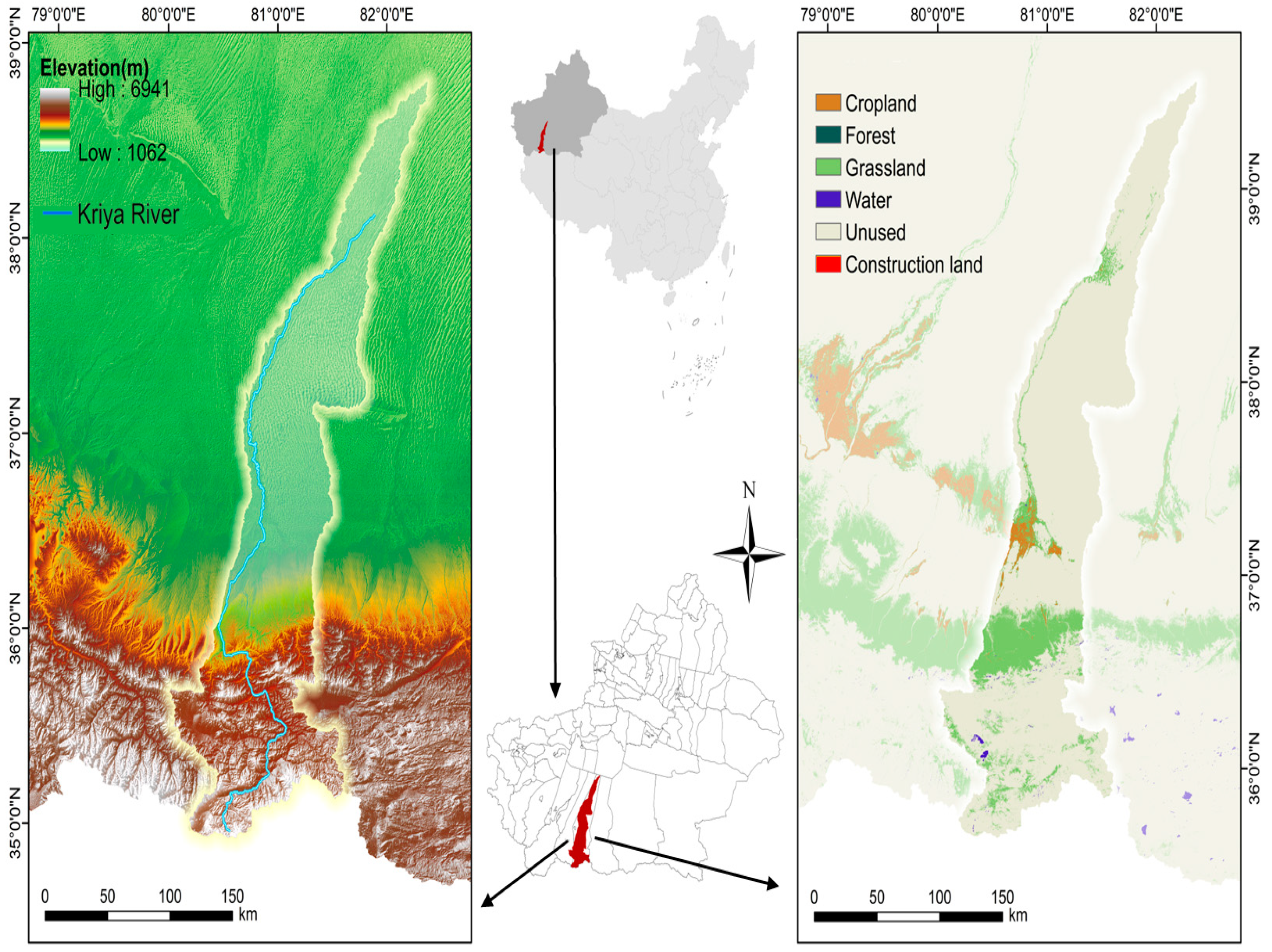
2.1. Study Area

The Kriya River Basin (KRB, China, 35°14′ N–39°30′ N, 81°09′ E–82°14′ E, Figure 1) is situated at the southern edge of the Taklamakan Desert, at the northern foothills of the Kunlun Mountain Range, occupying a total land area of about 4 × 10⁴ km2 [46]. The KRB’s topography is characterized by highlands in the south and lowlands in the north, with pronounced vertical zonal contrasts throughout the entire landscape [47]. The region belongs to the typical warm temperate, continental, and arid desert climates, and is distinguished by a notable temperature variation between day and night, scanty precipitation, and strong evaporation [48]. The long-term effect of the continental climate and the geomorphological pattern of a mountain basin has led to the development of oasis–desert ecosystem, and its natural ecology is relatively fragile. In recent years, with climate change, land use change, urban expansion, and economic development, the interplay of natural and human factors has led to major changes in the ecological environment [49,50].

2.2. Data Sources

2.2.1. Meteorological Data

The meteorological data were taken from the Data Center for Resource and Environmental Science (https://www.resdc.cn/, accessed on 10 April 2023). The spatial resolution was 1 km. The potential evapotranspiration data were obtained from the National Tibetan Plateau Science Data Center (https://data.tpdc.ac.cn, accessed on 10 April 2023). The spatial resolution was 0.0083333° (approximately 1 km).

2.2.2. Soil, Elevation, and Land Use Data

The maximum rooting depth of the soil was derived from the China Depth to Bedrock map, with a spatial resolution of 100 m. The dataset was based on borehole logging data from China (approximately 6382 sites) (globalchange.bnu.edu.cn/research/cdtb.jsp, accessed on 9 April 2023).
The World Soil Database, created by the Food and Agriculture Organization of the United Nations (FAO) and the International Institute for Applied Systems Analysis (HWSD, Harmonized World Soil Database, https://www.fao.org/, accessed on 28 February 2023), was used to calculate plant available water capacity (PAWC).
A geospatial data cloud (https://www.gscloud.cn/, accessed on 9 April 2022) was used to obtain digital elevation model (DEM) data. Land use change (LUC) data were obtained from the annual dataset of land use and cover from 1985 to 2020, which was built by the team led by Professor Huang Xin from Wuhan University based on Landsat images on Google Earth Engine (CLCD https://doi.org/10.5194/essd-2021-7) [51].

2.2.3. Social Economic Data

Population density and gross domestic product (GDP) data were taken from the Data Center for Resource and Environmental Science (https://www.resdc.cn/, accessed on 14 March 2023). Water system and road vector data were taken from the National Catalog Service for Geographic Information (https://www.webmap.cn/, accessed on 14 March 2023). Refer to Table S1 of the Supplementary Material for detailed data sources.

2.3. Methods

2.3.1. Land Use Future Forecasting Based on the PLUS Model

The PLUS model is a new and modified CA (Cellular Automat) model constructed by the High-Performance Spatial Computational Intelligence Laboratory of China University of Geosciences (Wuhan) based on the FLUS model. It enables simulation of future LUCs based on existing land use types coupled with a Land Expansion Analysis Strategy (LEAS) and a CA model based on multitype stochastic patch seeding (CARS) [32]. Some previous models have many shortcomings, such as the inability to simulate multiple land use categories and multiple patches, the lack of spatial and temporal dynamics, or difficulty in dealing with fine patches. The PLUS model combines the advantages of other models while overcoming their shortcomings and improves the simulation ability of the outputs. It accurately models the spatial distribution by predicting land changes under future factor constraints. Based on the historical land use data of the KRB for the years 2000 and 2010, climate and environmental data such as soil type, average yearly temperature, average yearly precipitation, DEM, slope, and distance to water, as well as socioeconomic metrics such as population density, GDP, and distance to primary, secondary, and tertiary roads, simulations of land use in 2020 were generated, which were then compared and evaluated with actual land use data in 2020. Using the Kappa coefficient and overall accuracy as evaluation indices, we found that the outputs of the model were sufficiently precise, which suggested that the same approach could be used for predicting land use types in 2030.
The Kappa consistency test is a statistical method used to evaluate the consistency of classification results of two or more observers’ consistency. The Kappa coefficient is given by:
Kappa = PA PE 1 PE
where PA is the probability of observational agreement and PE is the probability of expected agreement. Kappa coefficient values range from −1 to 1.
The model accuracy was evaluated using overall accuracy (OA), which was calculated as follows:
OA = T A
where T is the number of correctly categorized positive sample pixels, and A is the number of all pixels. The Kappa coefficient for this study was 0.853 and the OA was 0.962, indicating high precision and high reliability.

2.3.2. Ecosystem Service Assessment Based on the InVEST Model

  • Water Yield (WY) Model
The calculation of the WY model is based on the principle of water balancing [52]. The amount of WY flowing through each grid cell is determined based on precipitation minus actual evapotranspiration [53]. The WY is given by:
  Y x = 1 AET x P x × P x  
where Yx is the yearly WY (mm) for raster x, Px is the yearly precipitation (mm) for pixels x, and AETx is the actual evapotranspiration (mm) for pixels x. Refer to Table S2 in the Supplementary Materials for the biophysical tables required for the water yield service module.
2.
Soil Conservation (SC) Model
The sediment delivery ratio calculates soil retention as the difference between soil erosion reduction and sediment retention [54], as follows:
  SDR x = RKLS x USLE x + SEDR x
  RKLS x = R x × K x × LS x
  USLE x = R x × K x × LS x × C x × P x
R x = 0.0534 × P 1.6548
K x = 0.01383 + 0.51575 × K E P I C × 0.1317  
  K EPIC = 0.2 + 0.3 exp - 0.0256 SAND 1 SILT 100 ×   SILT CLAY + SILT 0.3 × 1 0.25 C C + exp ( 3.72 - 2.95 C ) × 1 0.7 SN SN + exp ( 22.9 SN - 5.51 )
where SDRx, USLEx, and SEDRx are the SC, potential erosion, and sediment retention for grid x, respectively; Rx, Kx, LSx, Cx, and Px are the rainfall erosivity factor, soil erodibility factor, slope length, gradient factor, and vegetation cover factor, respectively; USLEy is the actual erosion of upslope grid y; P is the annual precipitation; KEPIC is the soil erodibility factor calculated by the EPIC model; SAND is the sand content (%); SILT is the silt content (%); CLAY is the clay content (%); and C is the organic carbon content of the soil (%), where SN = 1 − (SAND/100). Kx are imperial units, multiplied by 0.1317 to convert to the International System of Units. Refer to Table S3 in the Supplementary Materials for the table of biophysical coefficients required for the Soil Conservation Module.
3.
Carbon Storage (CS) Model
The CS module sums the carbon densities of above-ground, below-ground, soil, and dead organic carbon of different land classes based on the classification of land use/cover to derive the carbon stock in the study area [55,56] as follows:
  C total = C above + C below + C soil + C dead
where Ctotal, Cabove, Cbelow, Csoil, and Cdead are total, above-ground, below-ground, soil, and dead organic carbon stocks, respectively. Refer to Table S6 in the Supplementary Materials for carbon density data required for carbon storage modules.
4.
Habitat Quality (HQ) Model
The HQ module evaluates the habitat quality of the study area by analyzing the extent to which threatening factors, such as anthropogenic or natural hazards, impact land use/vegetation patches at the regional landscape level [57,58]. The principle of calculation is as follows:
  Q xj = H j 1 D xj z D xj z + k z
where Qxj and Dxj are the HQ and habitat degradation index by grid x, respectively; Hj is the habitat suitability index; z is a normalized constant, which is dimensionless and has a default value of 2.5; and k is a half-saturation parameter that takes the value of 0.05.
D xj = r = 1 R y = 1 Y r W r r = 1 R W r r j i rxy β x S jr  
where R is the number of stressors; r is the stressor; y is the number of rasters for stressor r; Yr is the number of rasters occupied by the stressor; Wr is the stressor weight, with a range of 0–1; irxy is the effect (exponential or linear) of stressor r on each raster of the habitat; βx is the level of habitat resistance to perturbations; and Sjr is the relative sensitivity of different habitats to each stressor. For data on threat factors required for the Habitat Quality Module and the table of habitat sensitivity parameters, refer to Tables S4 and S5 in the Supplementary Materials.

2.3.3. Ecosystem Service Trade-Offs/Synergy Analysis

5.
Overall Benefits of ESs
Overall benefits reflect the whole range of benefits of several services and are dimensionless. There are connections between ESs, which often require a comprehensive analysis of multiple ESs to calculate their combined benefits [59]. Due to the different units of measurement for each ecosystem service, it is necessary to standardize the functions of different ecosystem services so that the value ranges from 0 to 1 [60]. The standardization formula is as follows:
ES bzi = ES i ES min ES max ES min
where ESbzi is the benefit after standardization of the ecosystem service; ESi is the functional value of the ecosystem service i; ESmin is the minimum value of ecosystem service i; and ESmax is the maximum value of ecosystem service i. The following is the overall benefit (OB) formula:
OB = 1 n i = 1 n ES bz
6.
ES Trade-offs and Synergies
This study was based on the evaluation results of four types of ESs, including WY, SC, CS, and HQ, using Spearman’s rank correlation coefficient (ρ) to identify the role relationships between services, in other words, whether there are synergies and trade-offs between two of the four ESs [61].
ρ = i = 1 n x i x ¯ y i y ¯ i = 1 n x i x ¯ 2 y i y ¯ 2
when ρ is 0, it indicates that there is no correlation between the two services. When ρ > 0, it is a positive correlation, showing that the two services have a synergistic relationship; in contrast, if ρ < 0, it is a negative correlation, indicating a trade-off relationship between the two services.
The software packages used in this paper included ArcGIS 10.8, InVEST 3.12.0, Origin 2021, PLUSv1.4, and IBM SPSS Statistics for Windows, version 27.0.

3. Results

3.1. LUC Historical Patterns and Future Developments

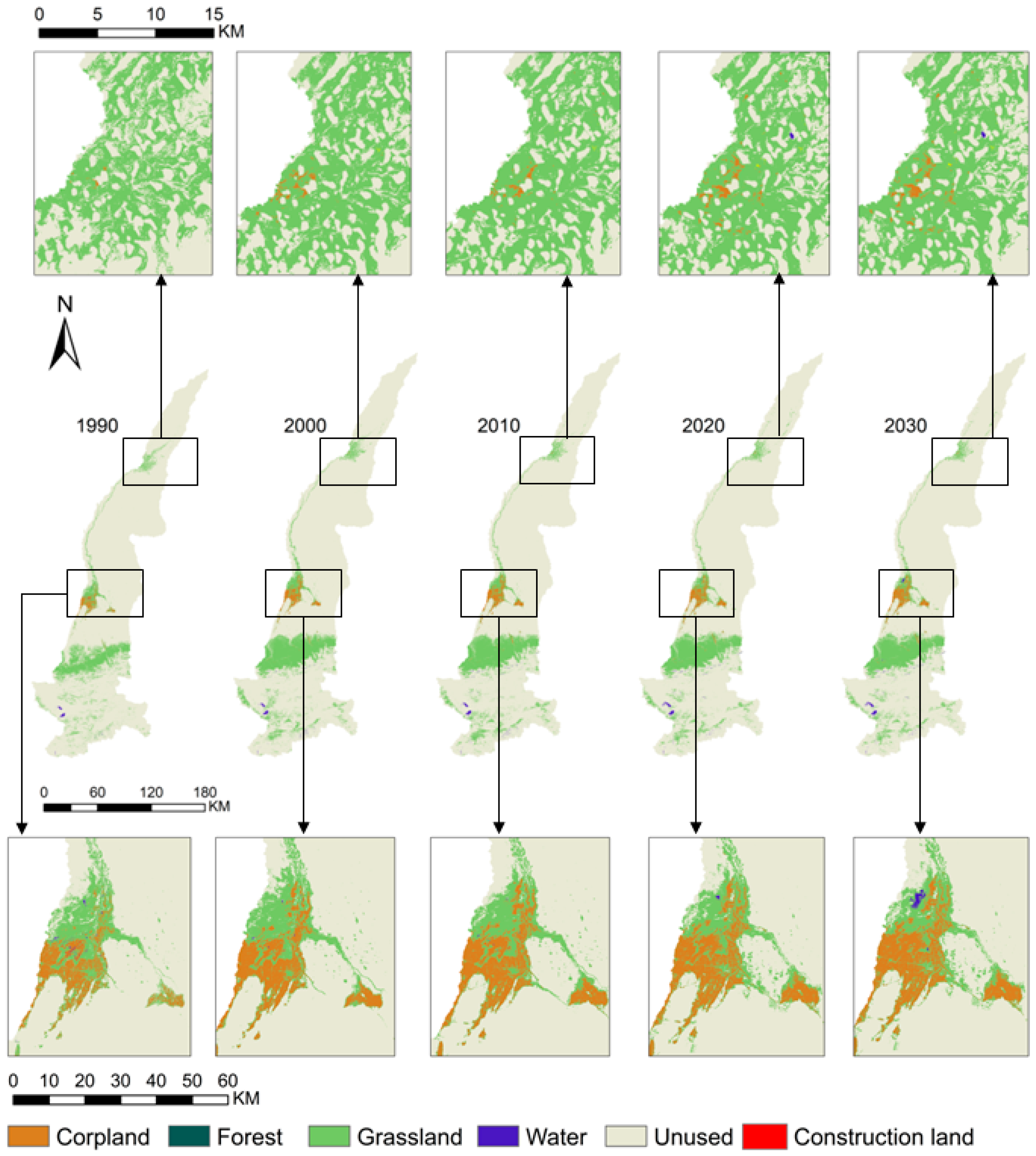
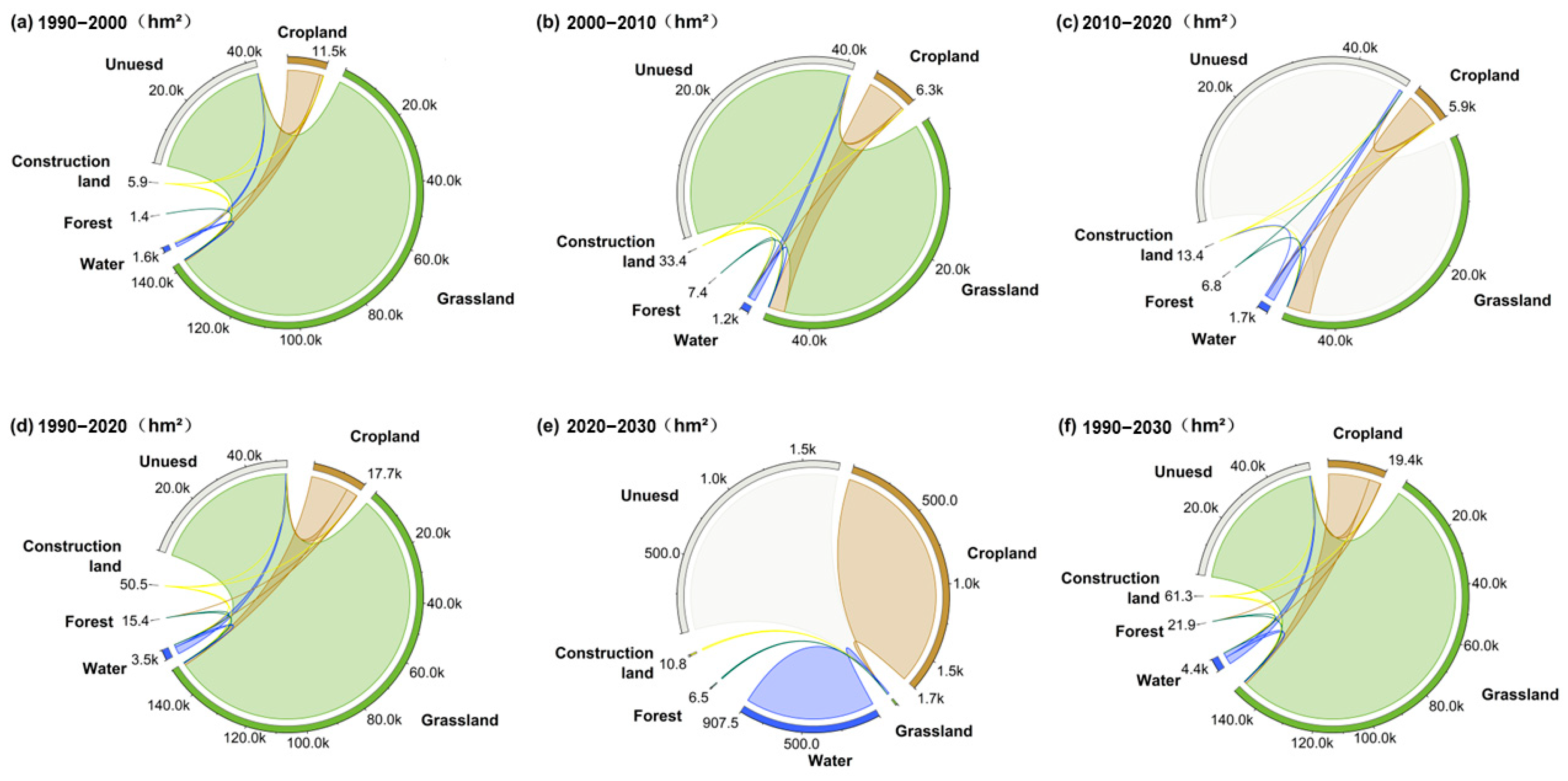
3.1.1. Analysis of Changes in Historical Patterns of Land Use in the Basin

Figure 2 shows the spatial distribution of land use in the KRB from 1990 to 2020, as well as simulated projections for 2030. The land use type of the basin was dominated by unused land and grassland, accounting for more than 90% of the area, of which unutilized land accounted for more than 85%. The Land Use Changes (LUCs) in the upstream, midstream, and downstream of the Kriya River Basin had significant spatial and temporal variations. Moreover, the upstream region, being the flow-producing area, contained watersheds and large grassland areas. Cropland and construction land were mainly distributed in the oasis area in the central part of the basin, while a smaller proportion of forestland was mainly distributed in the downstream area, and other land use types were sporadically distributed in the basin. Chord plots were used to represent the transfer matrix expressing land use changes in different periods (Figure 3). Chord plots provide a graphical representation that demonstrates the relationship between multiple land types. The width of the connecting lines represents the degree of relationship between the two types of data conversion, and the arrows represent the direction of land use transfer. In the period 1990–2000 (Figure 3a), cropland was transferred to grassland (246,410.13 hm2), grassland was mainly transferred to cropland and unused land (10,264.95 hm2 and 42,538.86 hm2, respectively), and water was mainly transferred to unused land (409.68 hm2), with most of the unused land shifting to grassland (141,212.5 hm2). In the period 2000–2010 (Figure 3b), the transfer of cropland to grassland was 2406.96 hm2, grassland to cropland was 5819 hm2, and grassland to unused land was 40,586.56 hm2. The transfer of water to unused land (343.44 hm2) was lower than that of the previous period and the transfer of unused land to grassland was 43,884.9 hm2. In 2010–2020 (Figure 3c), the transfer from cropland to grassland was 3837.78 hm2, from grassland to cropland was 5530.5 hm2 and to unused land was 47,597.58 hm2, from water to unused land was 570.78 hm2, and from unused land to grassland was 44,162 hm2. Total LUC from 1990 to 2020 (Figure 3d) was 20.46 × 10⁴ hm2, of which the unused land transfer area was the largest, decreasing by 10.23 × 10⁴ hm2 over 30 years and mainly shifting to grassland and cropland. This was followed by grassland, which increased by 8.28 × 10⁴ hm2, and was mainly converted from unused land. The rest of the land transfers were not obvious, but all showed an expansion trend. The period 2020–2030 was characterized mainly by grassland in circulation, and grassland mainly shifted to cropland and unused land. Overall, for the period 1990–2030 (Figure 3f), the largest amount of unused land was shifting, followed by grassland. Unused land mainly shifted to grassland, and grassland mainly shifted to cropland with unused land.

3.1.2. Simulated Prediction of Land Use Distribution Based on the PLUS Model

Based on the land use data in 2000 and 2010, the land use in 2020 was simulated using the PLUS model, and the results of the simulation were compared to the actual land use in 2020. The overall simulation accuracy was 0.962, and the Kappa coefficient was 0.853. Additionally, the high degree of spatial consistency of the simulation results demonstrated the PLUS model’s suitability for this study and its potential for predicting the distribution of land use in the future. According to the results of the prediction (Figure 2 and Figure 3), under the natural development scenario, the main land use type in the KRB in 2030 would remain unused land, and compared to 2020, all of the land use categories, except grassland, would show an increasing trend. The total extent of LUC would be 0.87 × 10⁴ hm2, and the amount of change would decrease in the order: grassland > unused land > cropland > water > construction land > forestland. The amount of grassland transferred would be 0.43 × 10⁴ hm2, mainly converted to cropland, unused land, and water. Cropland and unused land would continue to show an increasing trend, and a large amount of unused land would not be rationally utilized. The water area was projected to grow steadily, showing a positive trend, while the forestland area would slightly increase. According to the prediction results of the natural development scenario, if the land use categories maintained the trend in the future, the expansion of cropland and construction land would be accelerated, while ecological land, such as grassland and forestland, would be gradually reduced. Without reasonable human intervention, the study area’s future ecological safety would be threatened.

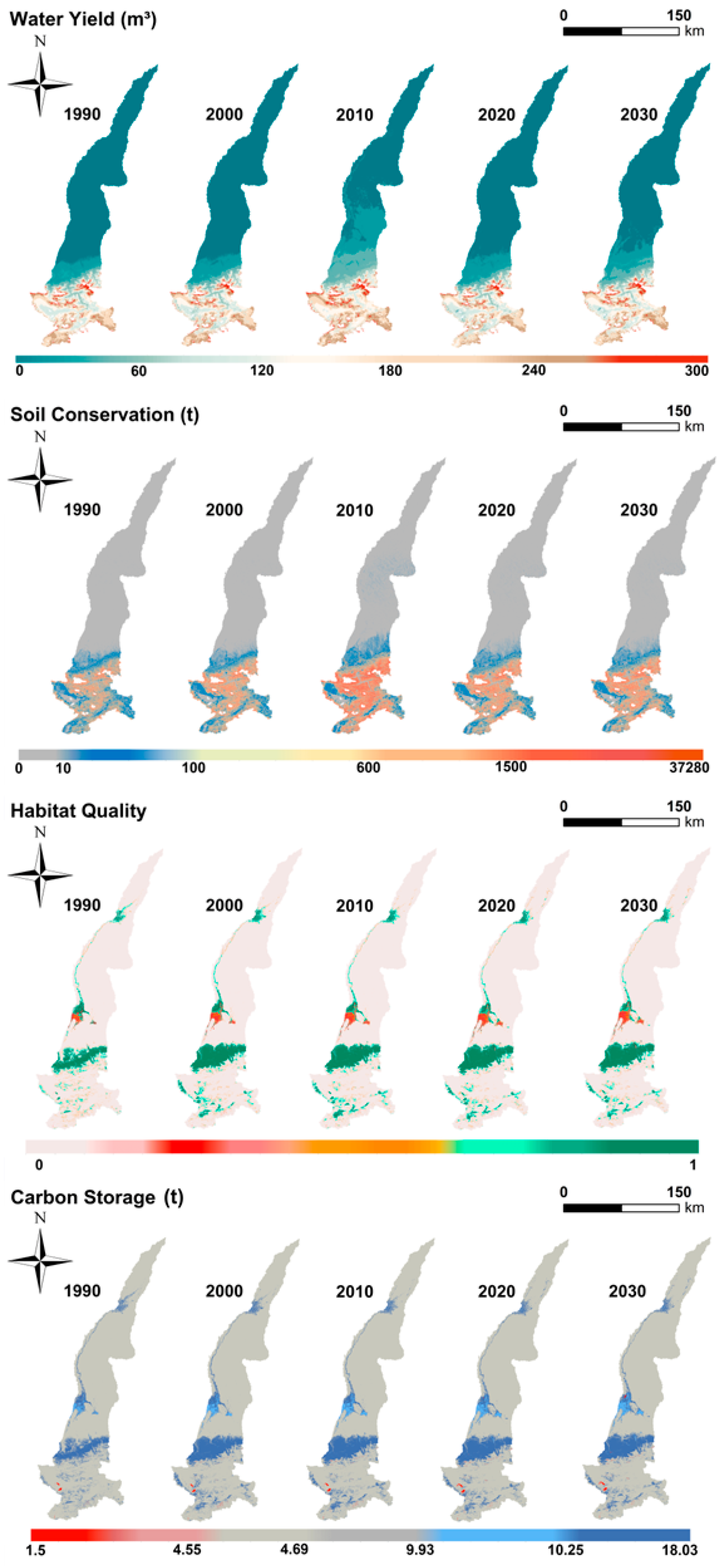
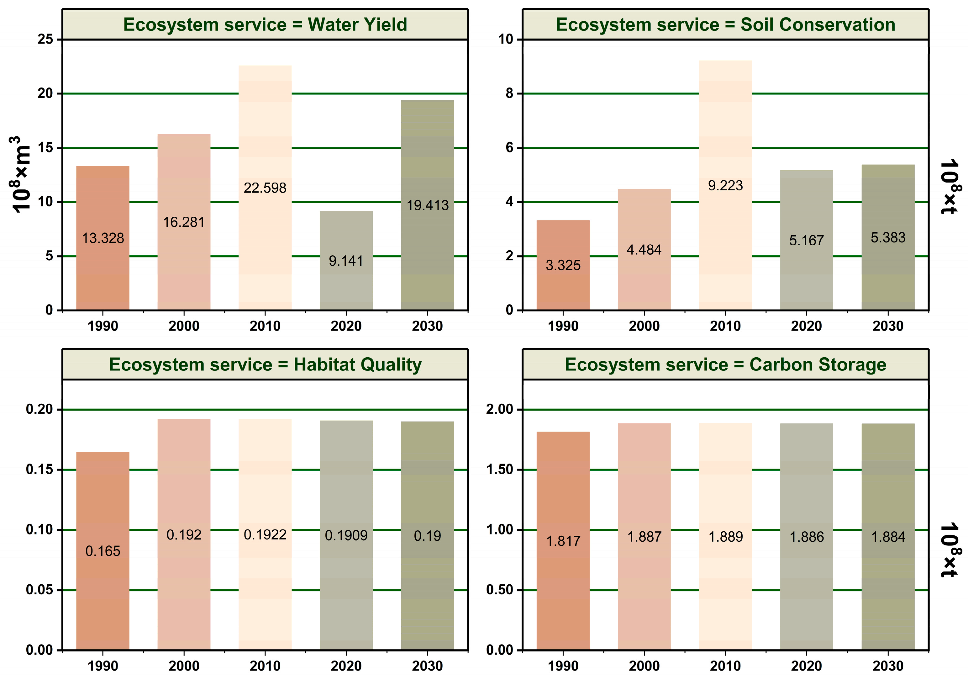
3.2. Spatial Distribution of Ecosystem Services

Figure 4 shows the spatial distribution of the four key ESs in the Kriya River Basin. From 1990 to 2020, the average annual water yield (WY) of the basin was concentrated in the upper reaches, exhibiting significant spatial diversity. The WY spatial pattern was characterized by a gradual decrease from the south to the north of the KRB. Higher WY was observed in the high-elevation areas of the mountainous regions, most of which yield more than 90 m3 of water per hectare. In the pre-mountain alluvial plain area, WY typically ranged between 10 and 60 m3 per hectare. The desert area in the midstream and downstream of the basin had the lowest water production, below 10 m3 per hectare, which was due to the larger distribution of precipitation in the watershed across the mountains. The spatial distribution pattern of WY in 2030 was projected to remain generally consistent with that of the past 30 years.
In terms of soil conservation (SC), high values were primarily observed in the southern areas with steeper slopes, while the northern areas with flat topography showed low SC values. This was because soil erosion occurs mainly in saline areas without vegetation cover, and the southern pre-mountain alluvial plains host a large amount of grassland, which is more effective in SC. The SC spatial distribution for 1990–2030 was consistent, with average SC decreasing from the southern region to the northern region.
The spatial pattern of habitat quality (HQ) in the Kriya River Basin was generally consistent with the LUC distribution. Areas with high HQ values corresponded spatially to grassland distribution areas, mainly owing to the abundance of annual precipitation, low evaporation, and low impact of human activities, with large amounts of original forestland and grassland. Areas of low HQ were distributed in construction land and cropland, spreading from the center to the surrounding area. The areas of low HQ covered 80% of the total area of the study area, which was related to the presence of a large area of the Gobi Desert in the upstream of the region and many deserts in the midstream and downstream.
The spatial distribution pattern of carbon storage (CS) in the Kriya River Basin exhibited only minor changes from 1990 to 2030. The high CS areas were mainly located in the pre-mountain alluvial plains and on both banks of the Kriya River, which have dense plant cover and a high carbon sequestration capability; the low-value CS regions were mainly located in lakes, construction land, and desert areas.

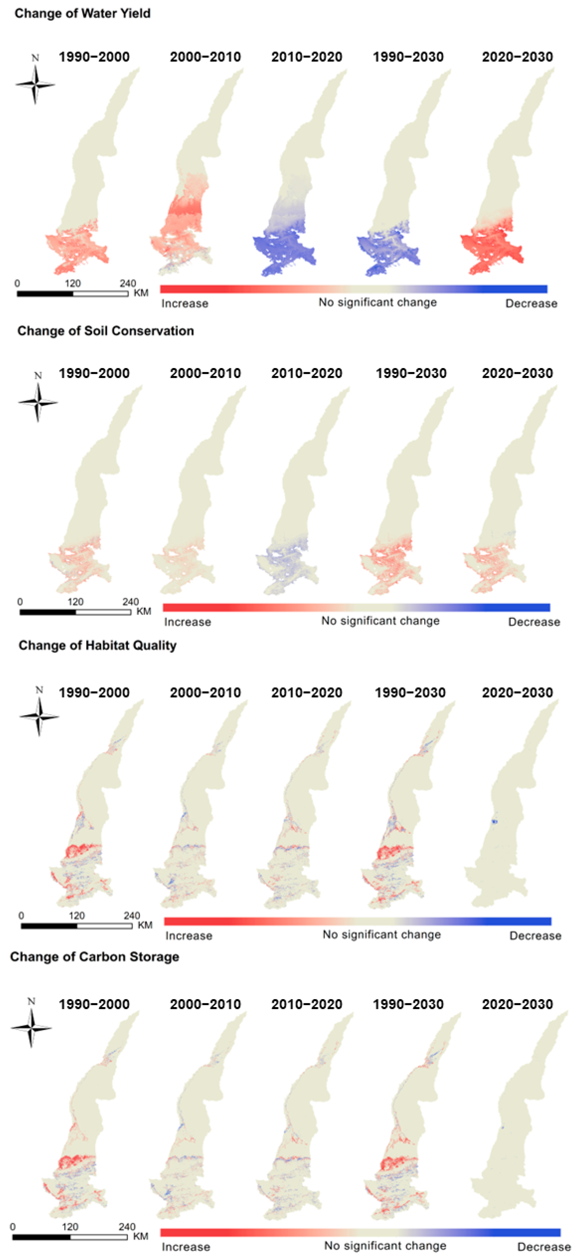
3.3. Characterization of Spatial and Temporal Changes in Ecosystem Services

Water yield (WY) in the Kriya River Basin fluctuated between 1990 and 2030 (Figure 5), being characterized by an initial increase, a decrease, and then another rise. Between 1990 and 2000, WY increased by 2.95 × 10⁸ m3, predominantly in mountainous regions. From 2000 to 2010, there was a significant rise of 6.32 × 10⁸ m3 in WY due to extreme precipitation in 2010, with the trend increasing from the upstream to the midstream regions of the basin (Figure 6). However, from 2010 to 2020, WY decreased by 13.46 × 10⁸ m3, with a greater reduction in mountainous areas. Overall, from 1990 to 2020, WY decreased by 4.19 × 10⁸ m3 in the upstream mountainous areas. Predictions for 2030, based on multiyear average precipitation and evapotranspiration data, indicated an increase in WY by 10.27 × 10⁸ m3.
SC in the Kriya River Basin followed a similar fluctuating pattern from 1990 to 2030 (Figure 5). The change was mostly in high-elevation mountains and pre-mountain alluvial plains (Figure 6). SC experienced an overall increase from 1990 to 2020, except for a decline from 2010 to 2020, influenced by precipitation erosion. The total increase in SC during this period was 1.84 × 10⁸ t, and the prediction for 2030 suggested a slight increase in SC compared to 2020.
The average habitat quality values for the Kriya River Basin for the years 1990–2030 were 0.1648, 0.192, 0.1922, 0.1909, and 0.19, respectively. Generally, HQ showed a trend of increasing and then slowly decreasing (Figure 5). The average habitat quality (HQ) for the Kriya River Basin increased from 1990 to 2000, slightly increased in 2010, and slightly decreased in 2020; a further slight decrease was projected for 2030. HQ decrease was mainly concentrated in construction land and cropland in the central region of the basin (Figure 6).
CS in the KRB was relatively stable between 1990 and 2030 (Figure 5). The total increase from 1990 to 2020 was 0.698 × 10⁸ t, with the most relevant growth from 1990 to 2000 due to an increase in grassland area (Figure 6). CS experienced slow growth followed by a minor decline from 2000 to 2020. Ongoing urban expansion was anticipated to lead to a continued decrease in total CS by 2030.

3.4. Ecosystem Services for Different Land Use Types

Table 1 shows the WY for different land use types. In 1990, the order of water production capacity per unit area for different land use types was forestland > grassland > unused land > construction land > cropland > water, with a difference of 769.220 m³ between the maximum and the minimum WY capacity per unit area. In 2020, the order of WY capacity per unit area for each land use type was forestland > grassland > unused land > cropland > construction land > water, with a difference of 482.95 m³ between the maximum and minimum values. In general, forests, grasslands, and unused land had a higher WY per unit area than other land types. In 1990 and 2020, the total water produced by different land use types was in the order of unused land > grassland > cropland > forestland > water > construction land, and the total amount of WY of unused land and grassland was much greater than that of other land use types (in both occurrences), which was directly related to the area proportion of these land use types.
Table 2 shows the SC for different land use types. In 1990 and 2020, the amount of SC per unit area of forestland was 612,322 t and decreased in the following order: forestland > grassland > water > unused land > construction land > cropland. The total SC for 1990 and 2020 was in the following order: unused land > grassland > water > forestland > cropland > construction land. In summary, areas with high vegetation cover typically had better water conservation, lower soil erosion, and higher SC, while areas with high human activities (croplands and construction lands) exacerbated soil erosion.
Table 3 shows the HQ of the different land use types. Between 1990 and 2020, the HQ index increased for forestland and grassland, decreased for cropland and water, and remained constant for unused land and construction land, with the largest increase in grassland and the largest decrease in water. The annual average HQ index of different land types increased in the order of forestland > grassland > water > cropland > unused land > construction land, which was mainly because forestland and grassland were further away from threat sources and had high habitat suitability, indicating that natural vegetation serves a very essential part in protecting ecosystem functionality.
Table 4 shows the CS of different land use types. The difference in CS per unit area for each land use type between 1990 and 2020 was relatively small. The highest CS per ha was recorded for forestland, which was followed by grassland and cropland, while the CS per unit area of construction land, unused land, and water was relatively small. The sum of CS of different land use types decreased in the following order: unused land > grassland > cropland > water > forestland > construction land. From 1990 to 2020, the increase in vegetation cover increased the total CS of the basin. This was due to a large amount of unused land being converted into grassland.
According to Table 1, Table 2, Table 3 and Table 4, it can be summarized that (i) the ESs of different land use types are obviously different, and overall, forestland and grassland are more favored than the other four land use types; (ii) for HQ and CS, cropland contributes more than construction land, whereas for WY and SC, construction land is better than cropland; and (iii) WY is highest in forestland, grassland, and unused land; SC is highest in forestland and grassland; HQ is highest in forestland, grassland, and watersheds; and cropland, forestland, and grassland have the highest CS.

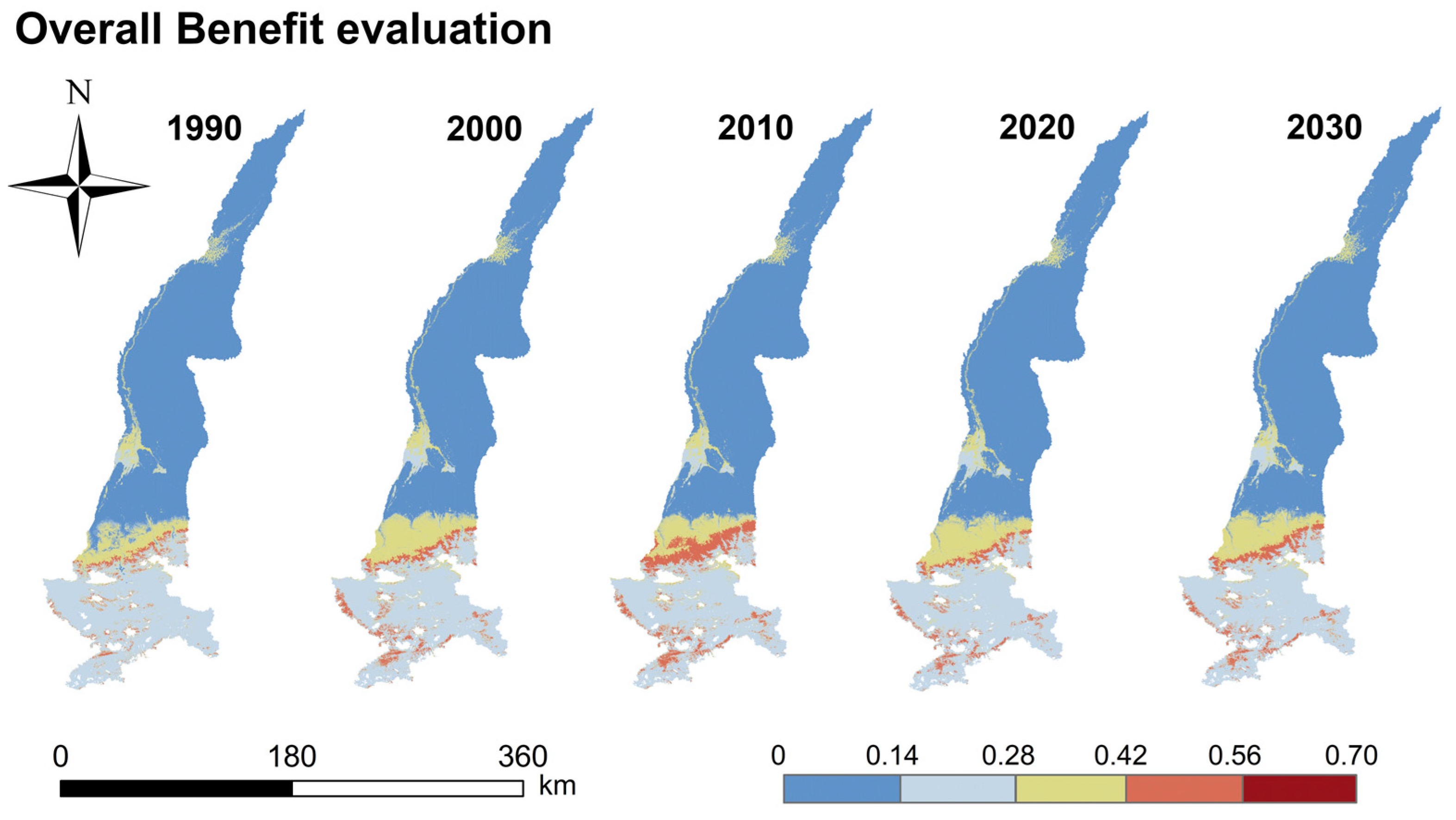
3.5. Trade-Off Analysis

All Spearman’s correlation coefficients between ESs in the KRB for 1990–2020 were significant at p = 0.01 (Table 5). The degree of correlation was divided into four categories: very low correlation (0–0.1), little correlation (0.1–0.3), moderate correlation (0.3–0.6), and strong correlation (0.6–1). In 1990, there was a trade-off between carbon storage and water yield (−0.003), and the rest of the services were synergistic with each other. In 2000, there was a trade-off between carbon storage and soil conservation (−0.002). The other services were synergistic, with the highest correlation observed between carbon storage and habitat quality (0.958). All services showed synergistic relationships in 2010. The year 2020 saw a negative correlation between habitat quality and water yield (−0.002), as well as a trade-off between carbon storage and water yield (−0.008). Positive correlations were projected between all services in 2030. Overall, carbon storage had the highest correlation with habitat quality, with the correlation remaining at 0.907 to 0.958 (strong correlation) between 1990 and 2030, followed by the relationship between water yield and soil conservation, which remained at 0.373 to 0.440 (moderate correlation). The correlations between the remaining services were low, particularly between water yield and habitat quality and between water yield and carbon storage.
Forestland exhibited the strongest capacity for all four ESs; grassland was second to forestland for all three services except CS; cropland had medium CS capacity and HQ and poor SC and WY capacity; water had good HQ and SC, showed a good growth trend, and almost no WY service and CS capacity; unused land showed better WY compared to the other three services and showed an overall stable growth trend; apart from weak CS capacity, the capacity of construction land for all other services was nearly negligible, and it was the land use type with the weakest ecosystem service functions among the six land use categories (Figure 7).

Overall Benefit Evaluation of Ecosystem Services

Figure 8 shows the spatial distribution of the overall benefit (OB) of ESs in the Kriya River Basin from 1990 to 2030. Overall, the spatial distribution pattern of the OB of ESs was basically the same in all periods, with high values in the south and low values in the north. The areas with high OB values were characterized by higher vegetation cover, higher elevation, and fewer human activities. The OB of ecosystem services in the basin from 1990 to 2020 showed a pattern of rising and then falling, with the highest value of the overall benefits reached in 2010, with an average value of 0.171, increasing by 0.029 compared to 1990. The year 2020 showed a decrease compared to 2010, but an increase of 0.012 compared to 1990, and OB was projected to continue to increase in 2030.

4. Discussion

4.1. Proposals for a Development Model

The results of this study indicate that areas with high ecosystem service values are ecological core areas of the watershed, and future planning should prioritize safeguarding of these ecological resources. The period 1990–2000 was the peak period of the increase in cropland and grassland, which coincided with western development and the policy of large-scale land reclamation, and later peaks in the period 2010–2020, which was the period when agricultural water conservancy facility projects increased and agricultural technologies such as plowing and irrigation substantially advanced. With the expansion of cropland areas, the phenomenon of alternating abandonment and reclamation has emerged. In the last 20 years, the state has rethought the construction of habitats, and activities such as returning farmland to forests and grasslands and reforestation have been increasing, gradually improving habitats in the Kriya River Basin. At the same time, increasing population pressure and the development of economic projects, such as mining (jade mining), hydraulic engineering (construction of the Giyin Reservoir in the upper part of the Kriya River Basin), the construction of a new highway, etc., have led to the destruction of natural vegetation and pastures. Planting a proportion of woodland and conserving water to irrigate both woodland and steeply sloping grassland will promote improvements in water, soil, and habitat quality, as well as carbon storage, maintaining the importance of the Kriya River Basin as an ecological security barrier. In areas where low values of ecosystem services are concentrated, the protection of forestland and grassland ecosystems should be strengthened, while the intensity of development of construction land should be slowed down to reduce the negative impacts of urban expansion on ecosystems. Considering the root causes of land use change, studies like [62,63] highlight the central role of socio-economic development, policy frameworks, and environmental factors. Socio-economic development particularly drives spatial and temporal changes in land use type, significantly altering the value of ESs. For instance, in the Kriya River Basin, the spatial distribution of the four ESs showed a high correlation with land use type, a phenomenon that was also observed in [64] in a different context.
For specific ecosystem services, extreme weather events, such as the high precipitation in 2010, significantly influence WY and SC in the Kriya River Basin. This observation aligns with the findings in [65], in which similar impacts were noted in other regions. Meanwhile, HQ and CS services maintained a steady growth trend, indicating that, unlike WY and SC, they are less immediately impacted by short-term climatic events but are more sensitive to long-term LUCs, as suggested in [66].
The basin is a complex system formed by multiple elements, including social-economic-natural elements, and the mode of its development and governance play a crucial role in its sustainable development [67]. The transition from unutilized land to grassland and cropland indicates a shift towards more intensive land use. This can have mixed effects on ecosystem services, depending on management practices.
The findings of this study indicate that modifications in LUCs will have a direct impact on the value of ecosystem services in the area, so land use should be rationally planned and controlled by zoning, clarifying the spatial distribution of the three categories of ecology, agriculture, and urbanization, rationally determining the scale of the new construction land and cropland, and avoiding the occupation of grasslands [68,69]. Forestland, which was the strongest contributor to the four ecosystem services per unit area, is extremely rare in the KRB; thus, the protection and restoration of forest resources should be increased and an ecological protection system for forestland and grassland resources should be built. This would not only protect ecosystem services but also help in preventing and controlling desertification [70,71]. To protect ecosystem services, we recommend encouraging sustainable farming methods to enhance SC and WY. Practices such as agroforestry, conservation tillage, and efficient irrigation can be beneficial. It is also important to implement urban planning strategies that incorporate green spaces and consider CS and HQ. Policies encouraging urban greenery, like rooftop gardens and city parks, can mitigate the impact of urban expansion. Initiatives to restore unutilized or degraded land can improve HQ and increase CS. Reforestation and grassland rehabilitation are key strategies. Given the expected increase in WY, it is of vital importance to develop appropriate strategies to sustainably manage water resources. This involves watershed management practices that ensure long-term water availability.

4.2. Deficiencies and Prospects

Land use change (LUC) is a complex process. Our study did not account for potential policy constraints, such as ecological protection red lines and land planning, in simulating future LUCs, introducing some uncertainty to our results.
Second, when using the InVEST model to assess ecosystem services, only four ecosystem services were selected without taking cultural services into account, and the setting of many parameters in the model was highly subjective and lacked measured data, for example, biophysical parameter tables, half-saturation parameters, etc. Therefore, the model relied on parameters from areas with similar environmental conditions, leading to potential biases in the accuracy of the results. In the future, if we can obtain real data from the study area, we will continue to complete the results of the study to reflect the actual local ecological environment more closely.
Correlation coefficients were used to analyze the trade-offs and synergies between ecosystem services. Although they can reflect the degree of trade-offs and synergies between ecosystem services, they are not able to detect the complexity of the relationships between more than two ecosystem services, and the trade-offs and synergies between ecosystem services are extremely complex [72]. Correlation coefficients do not adequately reflect the mechanisms inherent in trade-offs and synergies [73]. Further studies are needed to elaborate on the trade-offs and synergies among ecosystem services, for example, using spatial overlay analysis methods to visualize the spatially differentiated characteristics of trade-offs or synergistic relationships between multiple services [74].
However, although the results of this study cannot completely quantify the actual ES situation of the basin, they can reveal changing trends in various types of services and provide a scientific reference for the sustainable development of the basin and the establishment of ecological governance policies.

5. Conclusions

Land use in the Kriya River Basin is dominated by unused land and grassland. From 2020 to 2030, the trends in land use changes in the Kriya River Basin include an accelerated increase in construction land and cropland, slight increases in unused land, water, and forestland, and a decrease in grassland. WY showed a decreasing trend from 1990 to 2020, but in 2030 it is expected to increase. High-elevation areas in the southern mountains are particularly important for these ecosystem services. SC services have high values in the south and low values in the north, with a general increasing trend from 1990 to 2010, a decrease in 2020, followed by a slight increase in 2030. The spatial distribution pattern of HQ in the basin is spatially consistent with the distribution of LUCs, with forestland and grassland having higher HQ than construction land and cropland. However, the overall habitat quality is low due to the large proportion of unused land. The spatial distribution pattern of CS is closely related to vegetation and showed a positive trend from 1990 to 2020, but it is projected to decline slightly in 2030 due to accelerated urban expansion. There are synergistic relationships between WY and SC, WY and HQ, SC and HQ, SC and CS, and HQ and CS, while a modest trade-off is observed between WY and CS.

Supplementary Materials

The following supporting information can be downloaded at: https://www.mdpi.com/article/10.3390/su16052176/s1, Table S1: Data description and sources used; Table S2: Biophysical table of water yield; Table S3: Biophysical table of sediment delivery; Table S4: Table of threat factors data; Table S5: Table of habitat sensitivity parameters; Table S6: Above ground, below ground, soil, dead organic matter carbon stocks.

Author Contributions

Conceptualization, Y.L.; Data curation, Y.L., S.L. and K.X.; Formal analysis, Y.L.; Funding acquisition, S.L.; Investigation, Y.L.; Methodology, Y.L.; Project administration, S.L.; Resources, Y.L.; Software, Y.L.; Supervision, S.L. and K.X.; Validation, Y.L., S.L. and K.X.; Visualization, S.L. and K.X.; Writing—original draft, Y.L.; Writing—review & editing, S.L. and K.X. All authors have read and agreed to the published version of the manuscript.

Funding

This research was funded by Natural Science Foundation of Xinjiang Uygur Autonomous Region (2022D01C400).

Institutional Review Board Statement

Not applicable.

Informed Consent Statement

Not applicable.

Data Availability Statement

The data presented in this paper are contained within the article.

Conflicts of Interest

The authors declare no conflicts of interest.

References

  1. Costanza, R.; d’Arge, R.; de Groot, R.; Farber, S.; Grasso, M.; Hannon, B.; Limburg, K.; Naeem, S.; O’Neill, R.V.; Paruelo, J.; et al. The value of the world’s ecosystem services and natural capital. Nature 1997, 387, 253–260. [Google Scholar] [CrossRef]
  2. Fisher, B.; Turner, K.; Zylstra, M.; Brouwer, R.; Groot, R.D.; Farber, S.; Ferraro, P.; Green, R.; Hadley, D.; Harlow, J.; et al. Ecosystem Services and Economic Theory: Integration for Policy-Relevant Research. Ecol. Appl. 2008, 18, 2050–2067. [Google Scholar] [CrossRef] [PubMed]
  3. Kumar, P. The Economics of Ecosystems and Biodiversity: Ecological and Economic Foundations; Routledge: London, UK, 2012. [Google Scholar]
  4. Wallace, K.J. Classification of ecosystem services: Problems and solutions. Biol. Conserv. 2007, 139, 235–246. [Google Scholar] [CrossRef]
  5. Haines-Young, R.; Potschin, M. The links between biodiversity, ecosystem services and human well-being. In Ecosystem Ecology; Cambridge University Press: Cambridge, UK, 2010; pp. 110–139. [Google Scholar]
  6. Liu, M.; Wei, H.; Dong, X.; Wang, X.-C.; Zhao, B.; Zhang, Y. Integrating Land Use, Ecosystem Service, and Human Well-Being: A Systematic Review. Sustainability 2022, 14, 6926. [Google Scholar] [CrossRef]
  7. Fletcher, R.; Baulcomb, C.; Hall, C.; Hussain, S. Revealing marine cultural ecosystem services in the Black Sea. Mar. Policy 2014, 50, 151–161. [Google Scholar] [CrossRef]
  8. Reid, W.V.; Mooney, H.A.; Cropper, A.; Capistrano, D.; Carpenter, S.R.; Chopra, K.; Dasgupta, P.; Dietz, T.; Duraiappah, A.K.; Hassan, R.; et al. Ecosystems and Human Well-Being—Synthesis: A Report of the Millennium Ecosystem Assessment; Island Press: Washington, DC, USA, 2005. [Google Scholar]
  9. Assessment, M.E. Ecosystems and Human Well-Being; Island Press: Washington, DC, USA, 2005; Volume 5. [Google Scholar]
  10. Su, C.-H.; Fu, B.-J.; He, C.-S.; Lü, Y.-H. Variation of ecosystem services and human activities: A case study in the Yanhe Watershed of China. Acta Oecol. 2012, 44, 46–57. [Google Scholar] [CrossRef]
  11. Díaz, S.; Quétier, F.; Cáceres, D.M.; Trainor, S.F.; Pérez-Harguindeguy, N.; Bret-Harte, M.S.; Finegan, B.; Peña-Claros, M.; Poorter, L. Linking functional diversity and social actor strategies in a framework for interdisciplinary analysis of nature’s benefits to society. Proc. Natl. Acad. Sci. USA 2011, 108, 895–902. [Google Scholar] [CrossRef]
  12. Wang, X.; Dong, X.; Liu, H.; Wei, H.; Fan, W.; Lu, N.; Xu, Z.; Ren, J.; Xing, K. Linking land use change, ecosystem services and human well-being: A case study of the Manas River Basin of Xinjiang, China. Ecosyst. Serv. 2017, 27, 113–123. [Google Scholar] [CrossRef]
  13. Carpenter, S.R.; Mooney, H.A.; Agard, J.; Capistrano, D.; DeFries, R.S.; Díaz, S.; Dietz, T.; Duraiappah, A.K.; Oteng-Yeboah, A.; Pereira, H.M.; et al. Science for managing ecosystem services: Beyond the Millennium Ecosystem Assessment. Proc. Natl. Acad. Sci. USA 2009, 106, 1305–1312. [Google Scholar] [CrossRef] [PubMed]
  14. Douvere, F. The importance of marine spatial planning in advancing ecosystem-based sea use management. Mar. Policy 2008, 32, 762–771. [Google Scholar] [CrossRef]
  15. Fu, B.; Tian, T.; Liu, Y.; Zhao, W. New Developments and Perspectives in Physical Geography in China. Chin. Geogr. Sci. 2019, 29, 363–371. [Google Scholar] [CrossRef]
  16. Chen, S.; Chen, J.; Jiang, C.; Yao, R.T.; Xue, J.; Bai, Y.; Wang, H.; Jiang, C.; Wang, S.; Zhong, Y.; et al. Trends in Research on Forest Ecosystem Services in the Most Recent 20 Years: A Bibliometric Analysis. Forests 2022, 13, 1087. [Google Scholar] [CrossRef]
  17. Wood, S.L.R.; Jones, S.K.; Johnson, J.A.; Brauman, K.A.; Chaplin-Kramer, R.; Fremier, A.; Girvetz, E.; Gordon, L.J.; Kappel, C.V.; Mandle, L.; et al. Distilling the role of ecosystem services in the Sustainable Development Goals. Ecosyst. Serv. 2018, 29, 70–82. [Google Scholar] [CrossRef]
  18. Chen, D.; Zhao, Q.; Jiang, P.; Li, M. Incorporating ecosystem services to assess progress towards sustainable development goals: A case study of the Yangtze River Economic Belt, China. Sci. Total Environ. 2022, 806, 151277. [Google Scholar] [CrossRef] [PubMed]
  19. Zheng, D.; Wang, Y.; Hao, S.; Xu, W.; Lv, L.; Yu, S. Spatial-temporal variation and tradeoffs/synergies analysis on multiple ecosystem services: A case study in the Three-River Headwaters region of China. Ecol. Indic. 2020, 116, 106494. [Google Scholar] [CrossRef]
  20. Raymond, C.M.; Bryan, B.A.; MacDonald, D.H.; Cast, A.; Strathearn, S.; Grandgirard, A.; Kalivas, T. Mapping community values for natural capital and ecosystem services. Ecol. Econ. 2009, 68, 1301–1315. [Google Scholar] [CrossRef]
  21. Cord, A.F.; Bartkowski, B.; Beckmann, M.; Dittrich, A.; Hermans-Neumann, K.; Kaim, A.; Lienhoop, N.; Locher-Krause, K.; Priess, J.; Schröter-Schlaack, C.; et al. Towards systematic analyses of ecosystem service trade-offs and synergies: Main concepts, methods and the road ahead. Ecosyst. Serv. 2017, 28, 264–272. [Google Scholar] [CrossRef]
  22. Liu, Y.; Yuan, X.; Li, J.; Qian, K.; Yan, W.; Yang, X.; Ma, X. Trade-offs and synergistic relationships of ecosystem services under land use change in Xinjiang from 1990 to 2020: A Bayesian network analysis. Sci. Total Environ. 2023, 858, 160015. [Google Scholar] [CrossRef]
  23. Locatelli, B.; Imbach, P.; Wunder, S. Synergies and trade-offs between ecosystem services in Costa Rica. Environ. Conserv. 2013, 41, 27–36. [Google Scholar] [CrossRef]
  24. Kirchner, M.; Schmidt, J.; Kindermann, G.; Kulmer, V.; Mitter, H.; Prettenthaler, F.; Rüdisser, J.; Schauppenlehner, T.; Schönhart, M.; Strauss, F.; et al. Ecosystem services and economic development in Austrian agricultural landscapes—The impact of policy and climate change scenarios on trade-offs and synergies. Ecol. Econ. 2015, 109, 161–174. [Google Scholar] [CrossRef]
  25. Shen, J.; Li, S.; Liang, Z.; Liu, L.; Li, D.; Wu, S. Exploring the heterogeneity and nonlinearity of trade-offs and synergies among ecosystem services bundles in the Beijing-Tianjin-Hebei urban agglomeration. Ecosyst. Serv. 2020, 43, 101103. [Google Scholar] [CrossRef]
  26. Wang, L.J.; Ma, S.; Qiao, Y.P.; Zhang, J.C. Simulating the Impact of Future Climate Change and Ecological Restoration on Trade-Offs and Synergies of Ecosystem Services in Two Ecological Shelters and Three Belts in China. Int. J. Environ. Res. Public Health 2020, 17, 7849. [Google Scholar] [CrossRef]
  27. Bengtsson, J.; Bullock, J.M.; Egoh, B.; Everson, C.; Everson, T.; O’Connor, T.; O’Farrell, P.J.; Smith, H.G.; Lindborg, R. Grasslands-more important for ecosystem services than you might think. Ecosphere 2019, 10, e02582. [Google Scholar] [CrossRef]
  28. Lawler, J.J.; Lewis, D.J.; Nelson, E.; Plantinga, A.J.; Polasky, S.; Withey, J.C.; Helmers, D.P.; Martinuzzi, S.; Pennington, D.; Radeloff, V.C. Projected land-use change impacts on ecosystem services in the United States. Proc. Natl. Acad. Sci. USA 2014, 111, 7492–7497. [Google Scholar] [CrossRef]
  29. Geneletti, D. Assessing the impact of alternative land-use zoning policies on future ecosystem services. Environ. Impact Assess. Rev. 2013, 40, 25–35. [Google Scholar] [CrossRef]
  30. van Oudenhoven, A.P.E.; Petz, K.; Alkemade, R.; Hein, L.; de Groot, R.S. Framework for systematic indicator selection to assess effects of land management on ecosystem services. Ecol. Indic. 2012, 21, 110–122. [Google Scholar] [CrossRef]
  31. Jia, X.; Fu, B.; Feng, X.; Hou, G.; Liu, Y.; Wang, X. The tradeoff and synergy between ecosystem services in the Grain-for-Green areas in Northern Shaanxi, China. Ecol. Indic. 2014, 43, 103–113. [Google Scholar] [CrossRef]
  32. Liang, X.; Guan, Q.; Clarke, K.C.; Liu, S.; Wang, B.; Yao, Y. Understanding the drivers of sustainable land expansion using a patch-generating land use simulation (PLUS) model: A case study in Wuhan, China. Comput. Environ. Urban Syst. 2021, 85, 101569. [Google Scholar] [CrossRef]
  33. Li, X.; Liu, Z.; Li, S.; Li, Y. Multi-Scenario Simulation Analysis of Land Use Impacts on Habitat Quality in Tianjin Based on the PLUS Model Coupled with the InVEST Model. Sustainability 2022, 14, 6923. [Google Scholar] [CrossRef]
  34. Wang, R.; Zhao, J.; Chen, G.; Lin, Y.; Yang, A.; Cheng, J. Coupling PLUS–InVEST Model for Ecosystem Service Research in Yunnan Province, China. Sustainability 2023, 15, 271. [Google Scholar] [CrossRef]
  35. Sun, X.; Crittenden, J.C.; Li, F.; Lu, Z.; Dou, X. Urban expansion simulation and the spatio-temporal changes of ecosystem services, a case study in Atlanta Metropolitan area, USA. Sci. Total Environ. 2018, 622–623, 974–987. [Google Scholar] [CrossRef]
  36. Sun, J.; Zhang, Y.; Qin, W.; Chai, G. Estimation and Simulation of Forest Carbon Stock in Northeast China Forestry Based on Future Climate Change and LUCC. Remote Sens. 2022, 14, 3653. [Google Scholar] [CrossRef]
  37. Xiao, D.; Chen, W. On the basic concepts and contents of ecological security. J. Appl. Ecol. 2002, 13, 354–358. [Google Scholar]
  38. Xue, X.; Liao, J.; Hsing, Y.; Huang, C.; Liu, F. Policies, Land Use, and Water Resource Management in an Arid Oasis Ecosystem. Environ. Manag. 2015, 55, 1036–1051. [Google Scholar] [CrossRef]
  39. Feng, W.; Liu, Y.; Qu, L. Effect of land-centered urbanization on rural development: A regional analysis in China. Land Use Policy 2019, 87, 104072. [Google Scholar] [CrossRef]
  40. Hu, K.; Ailihazi, W.; Danierhan, S. Ecological Base Flow Characteristics of Typical Rivers on the North Slope of Kunlun Mountains under Climate Change. Atmosphere 2023, 14, 842. [Google Scholar] [CrossRef]
  41. Peng, L.; Shi, Q.-D.; Wan, Y.-B.; Shi, H.-B.; Kahaer, Y.-J.; Abudu, A. Impact of Flooding on Shallow Groundwater Chemistry in the Taklamakan Desert Hinterland: Remote Sensing Inversion and Geochemical Methods. Water 2022, 14, 1724. [Google Scholar] [CrossRef]
  42. Hou, Y.; Chen, Y.; Ding, J.; Li, Z.; Li, Y.; Sun, F. Ecological Impacts of Land Use Change in the Arid Tarim River Basin of China. Remote Sens. 2022, 14, 1894. [Google Scholar] [CrossRef]
  43. Xu, Y.; Gao, Y. An analysis of water resource characteristics of the rivers in the northern slope of the Kunlun Mountains. Chin. Geogr. Sci. 1995, 5, 365–373. [Google Scholar] [CrossRef]
  44. Hou, Y.; Chen, Y.; Li, Z.; Li, Y.; Sun, F.; Zhang, S.; Wang, C.; Feng, M. Land Use Dynamic Changes in an Arid Inland River Basin Based on Multi-Scenario Simulation. Remote Sens. 2022, 14, 2797. [Google Scholar] [CrossRef]
  45. Hou, Y.; Chen, Y.; Li, Z.; Wang, Y. Changes in Land Use Pattern and Structure under the Rapid Urbanization of the Tarim River Basin. Land 2023, 12, 693. [Google Scholar] [CrossRef]
  46. Leng, X.; Feng, X.; Fu, B.; Zhang, Y. The Spatiotemporal Regime of Glacier Runoff in Oases Indicates the Potential Climatic Risk in Dryland Areas of China. Hydrol. Earth Syst. Sci. Discuss. 2021, 2021, 1–52. [Google Scholar] [CrossRef]
  47. Saimaiti, A.; Fu, C.; Song, Y.; Shukurov, N. Spatial Distribution, Material Composition and Provenance of Loess in Xinjiang, China: Progress and Challenges. Atmosphere 2022, 13, 1790. [Google Scholar] [CrossRef]
  48. Ye, Z.; Chen, Y.; Li, W. Ecological water rights and water-resource exploitation in the three headwaters of the Tarim River. Quat. Int. 2014, 336, 20–25. [Google Scholar] [CrossRef]
  49. Wan, Y.; Shi, Q.; Dai, Y.; Marhaba, N.; Peng, L.; Peng, L.; Shi, H. Water Use Characteristics of Populus euphratica Oliv. and Tamarix chinensis Lour. at Different Growth Stages in a Desert Oasis. Forests 2022, 13, 236. [Google Scholar] [CrossRef]
  50. Wang, N.; Guo, Y.; Wei, X.; Zhou, M.; Wang, H.; Bai, Y. UAV-based remote sensing using visible and multispectral indices for the estimation of vegetation cover in an oasis of a desert. Ecol. Indic. 2022, 141, 109155. [Google Scholar] [CrossRef]
  51. Yang, J.; Huang, X. The 30 m annual land cover dataset and its dynamics in China from 1990 to 2019. Earth Syst. Sci. Data 2021, 13, 3907–3925. [Google Scholar] [CrossRef]
  52. Webster, P.J. Climate and life. M. I. Budyko (David H. Miller, Translator). Academic Press, New York, $35.00. Quat. Res. 1976, 6, 461–463. [Google Scholar] [CrossRef]
  53. Yang, D.; Liu, W.; Tang, L.; Chen, L.; Li, X.; Xu, X. Estimation of water provision service for monsoon catchments of South China: Applicability of the InVEST model. Landsc. Urban Plan. 2019, 182, 133–143. [Google Scholar] [CrossRef]
  54. Liu, H.; Liu, Y.; Wang, K.; Zhao, W. Soil conservation efficiency assessment based on land use scenarios in the Nile River Basin. Ecol. Indic. 2020, 119, 106864. [Google Scholar] [CrossRef]
  55. Zhu, G.; Qiu, D.; Zhang, Z.; Sang, L.; Liu, Y.; Wang, L.; Zhao, K.; Ma, H.; Xu, Y.; Wan, Q. Land-use changes lead to a decrease in carbon storage in arid region, China. Ecol. Indic. 2021, 127, 107770. [Google Scholar] [CrossRef]
  56. Lai, L.; Huang, X.; Yang, H.; Chuai, X.; Zhang, M.; Zhong, T.; Chen, Z.; Chen, Y.; Wang, X.; Thompson, J.R. Carbon emissions from land-use change and management in China between 1990 and 2010. Sci. Adv. 2016, 2, e1601063. [Google Scholar] [CrossRef] [PubMed]
  57. Sharp, R.; Tallis, H.; Ricketts, T.; Guerry, A.; Wood, S.A.; Chaplin-Kramer, R.; Nelson, E.; Ennaanay, D.; Wolny, S.; Olwero, N. InVEST User’s Guide; The Natural Capital Project: Stanford, CA, USA, 2014. [Google Scholar]
  58. Sallustio, L.; De Toni, A.; Strollo, A.; Di Febbraro, M.; Gissi, E.; Casella, L.; Geneletti, D.; Munafo, M.; Vizzarri, M.; Marchetti, M. Assessing habitat quality in relation to the spatial distribution of protected areas in Italy. J. Environ. Manag. 2017, 201, 129–137. [Google Scholar] [CrossRef]
  59. Chen, X.; Chen, Y.; Shimizu, T.; Niu, J.; Nakagami, K.; Qian, X.; Jia, B.; Nakajima, J.; Han, J.; Li, J. Water resources management in the urban agglomeration of the Lake Biwa region, Japan: An ecosystem services-based sustainability assessment. Sci. Total Environ. 2017, 586, 174–187. [Google Scholar] [CrossRef] [PubMed]
  60. Kremen, C. Managing ecosystem services: What do we need to know about their ecology? Ecol. Lett. 2005, 8, 468–479. [Google Scholar] [CrossRef]
  61. Xu, S.; Liu, Y. Associations among ecosystem services from local perspectives. Sci. Total Environ. 2019, 690, 790–798. [Google Scholar] [CrossRef] [PubMed]
  62. Lambin, E.F.; Meyfroidt, P. Land use transitions: Socio-ecological feedback versus socio-economic change. Land Use Policy 2010, 27, 108–118. [Google Scholar] [CrossRef]
  63. Popp, A.; Calvin, K.; Fujimori, S.; Havlik, P.; Humpenöder, F.; Stehfest, E.; Bodirsky, B.L.; Dietrich, J.P.; Doelmann, J.C.; Gusti, M. Land-use futures in the shared socio-economic pathways. Glob. Environ. Chang. 2017, 42, 331–345. [Google Scholar] [CrossRef]
  64. Paudyal, K.; Baral, H.; Bhandari, S.P.; Bhandari, A.; Keenan, R.J. Spatial assessment of the impact of land use and land cover change on supply of ecosystem services in Phewa watershed, Nepal. Ecosyst. Serv. 2019, 36, 100895. [Google Scholar] [CrossRef]
  65. Dai, X.; Wang, L.; Li, X.; Gong, J.; Cao, Q. Characteristics of the extreme precipitation and its impacts on ecosystem services in the Wuhan Urban Agglomeration. Sci. Total Environ. 2023, 864, 161045. [Google Scholar] [CrossRef]
  66. Lin, Y.-P.; Chen, C.-J.; Lien, W.-Y.; Chang, W.-H.; Petway, J.R.; Chiang, L.-C. Landscape conservation planning to sustain ecosystem services under climate change. Sustainability 2019, 11, 1393. [Google Scholar] [CrossRef]
  67. Wang, B.; Wang, H.; Zeng, X.; Li, B. Towards a Better Understanding of Social-Ecological Systems for Basin Governance: A Case Study from the Weihe River Basin, China. Sustainability 2022, 14, 4922. [Google Scholar] [CrossRef]
  68. He, Q.; Tan, S.; Yin, C.; Zhou, M. Collaborative optimization of rural residential land consolidation and urban construction land expansion: A case study of Huangpi in Wuhan, China. Comput. Environ. Urban Syst. 2019, 74, 218–228. [Google Scholar] [CrossRef]
  69. Xie, H.; He, Y.; Choi, Y.; Chen, Q.; Cheng, H. Warning of negative effects of land-use changes on ecological security based on GIS. Sci. Total Environ. 2020, 704, 135427. [Google Scholar] [CrossRef]
  70. Amogne, A.E. Forest resource management systems in Ethiopia: Historical perspective. Int. J. Biodivers. Conserv. 2014, 6, 121–131. [Google Scholar] [CrossRef]
  71. Xu, S.; Wang, X.; Ma, X.; Gao, S. Risk Assessment and Prediction of Soil Water Erosion on the Middle Northern Slope of Tianshan Mountain. Sustainability 2023, 15, 4826. [Google Scholar] [CrossRef]
  72. Jopke, C.; Kreyling, J.; Maes, J.; Koellner, T. Interactions among ecosystem services across Europe: Bagplots and cumulative correlation coefficients reveal synergies, trade-offs, and regional patterns. Ecol. Indic. 2015, 49, 46–52. [Google Scholar] [CrossRef]
  73. Lin, S.; Wu, R.; Yang, F.; Wang, J.; Wu, W. Spatial trade-offs and synergies among ecosystem services within a global biodiversity hotspot. Ecol. Indic. 2018, 84, 371–381. [Google Scholar] [CrossRef]
  74. Dade, M.C.; Mitchell, M.G.E.; McAlpine, C.A.; Rhodes, J.R. Assessing ecosystem service trade-offs and synergies: The need for a more mechanistic approach. Ambio 2019, 48, 1116–1128. [Google Scholar] [CrossRef] [PubMed]
Figure 1. The Kriya River Basin (China). The left panel illustrates the elevation of the study area, whereas the right panel presents the distribution of land use categories as recorded in 2020.
Sustainability 16 02176 g001
Figure 2. Distribution of past land uses (from 1990 to 2020) and projections for 2030 based on the PLUS model in the Kriya River Basin (China). To better illustrate the changes, two areas, representative of the northern and southern sectors, are shown on a smaller scale.
Sustainability 16 02176 g002
Figure 3. Matrix chord diagrams of land use transfers in the Kriya River Basin (China) from 1990 to 2030.
Sustainability 16 02176 g003
Figure 4. Spatial distribution of four ecosystem services in the Kriya River Basin (China) in 1990, 2000, 2010, 2020, and 2030.
Sustainability 16 02176 g004
Figure 5. Temporal changes in four ecosystem services in the Kriya River Basin (China) in 1990, 2000, 2010, 2020, and 2030.
Sustainability 16 02176 g005
Figure 6. Spatial changes in four ecosystem services in the Kriya River Basin (China) in 1990, 2000, 2010, 2020, and 2030.
Sustainability 16 02176 g006
Figure 7. Standardized ecosystem service functions for different land types in the Kriya River Basin (China) in 1990, 2000, 2010, 2020, and 2030.
Sustainability 16 02176 g007
Figure 8. Overall benefits of ecosystem services in the Kriya River Basin (China) in 1990, 2000, 2010, 2020, and 2030.
Sustainability 16 02176 g008
Table 1. Water yield (WY) for different land use types in 1990 and 2020 in the Kriya River Basin (China).
WY per Unit Area (m3/hm2)Total WY (m3 × 104)
Year1990202019902020
Cropland4.28311.0378.19039.813
Forest769.424482.9911.9531.965
Grassland511.405346.09014,852.93912,915.658
Water0.2040.0410.0790.026
Unused477.236329.838118,438.62678,484.066
Construction land36.7155.0770.0600.034
Table 2. Soil conservation (SC) for different land use types in 1990 and 2020 in the Kriya River Basin (China).
SC per Unit Area (t/hm2)Total SC (t × 104)
Year1990202019902020
Cropland0.2170.7090.4152.557
Forest612.539796.1271.5553.239
Grassland187.963203.9205459.0857610.046
Water128.497397.09950.025254.893
Unused112.244184.86827,856.35443,988.903
Construction land0.4120.8080.000010.001
Table 3. Average habitat quality (HQ) for different land use types in 1990 and 2020 in the Kriya River Basin (China).
Year19902020
Cropland0.3280.313
Forest0.9660.967
Grassland0.8280.847
Water0.7470.708
Unused0.0880.088
Construction land0.0000.000
Table 4. Carbon storage (CS) for different land use types in 1990 and 2020 in the Kriya River Basin (China).
CS per Unit Area (t/hm2)Total CS (t × 104)
Year1990202019902020
Cropland124.2033124.2493237.502448.179
Forest222.3081223.77510.5640.91
Grassland128.8872128.88823743.3054809.943
Water18.932618.91667.371.214
Unused57.126557.124514,177.21613,592.553
Construction land60.955458.98740.10.395
Table 5. Trade-offs and synergies of ecosystem services in the Kriya River Basin (China) (1990–2030).
Water YieldSoil ConservationHabitat QualityCarbon Storage
1990
Water Yield1
Soil Conservation0.373 **1
Habitat Quality0.0020.040 **1
Carbon Storage−0.0030.034 *0.907 **1
2000
Water Yield1
Soil Conservation0.436 **1
Habitat Quality0.0150.0051
Carbon Storage0.013−0.0020.958 **1
2010
Water Yield1
Soil Conservation0.427 **1
Habitat Quality0.0510.0231
Carbon Storage0.049 **0.0190.950 **1
2020
Water Yield1
Soil Conservation0.440 **1
Habitat Quality−0.0020.0051
Carbon Storage−0.0080.0020.951 **1
2030
Water Yield1
Soil Conservation0.435 **1
Habitat Quality0.0150.0041
Carbon Storage0.0080.0010.949 **1
** significant at p < 0.001, * significant at p < 0.05.
Disclaimer/Publisher’s Note: The statements, opinions and data contained in all publications are solely those of the individual author(s) and contributor(s) and not of MDPI and/or the editor(s). MDPI and/or the editor(s) disclaim responsibility for any injury to people or property resulting from any ideas, methods, instructions or products referred to in the content.

