Study on Spatial and Temporal Changes in Landscape Ecological Risks and Indicator Weights: A Case Study of the Bailong River Basin

Abstract

The land use and ecological environment of the Bailong River Basin (BRB) have undergone significant changes in the context of developing urban–rural integration and ecological conservation in western China. As a key ecologically fragile area in the west region, a landscape ecological risk (LER) assessment can reflect the extent to which human activities and environmental changes threaten the ecosystems in the BRB. This study aims to explore the empowerment of indicator weights in an LER assessment. Landscape index weights and LER were analyzed based on land use data for three periods using objective and combined empowerment methods. It was found that the weighting results had apparent scale dependence, and the entropy weight method had the best results in indicator empowerment. From 2000–2020, the LER presented reduced risk, increased heterogeneity, and reduced aggregation. The shift from a medium-risk area to a lower-risk area was the primary transfer type of LER in the study area, and the LER showed a decreasing development trend. So far, research on weight empowerment in LER evaluations has been urgent. This study improved the landscape ecological risk assessment system by selecting an empowerment method that optimally takes into account scale dependence while providing valuable insights into the sustainability of the landscape in this watershed.

1. Introduction

The past 20 years have seen rapid economic development and new rural construction in Western China. The growing demands of the people for a better life have led to increasingly prominent conflicts between land supply and demand and agricultural production. In the western mountainous areas, the natural environment has been disturbed by human activities, resulting in a series of ecological and environmental problems such as land degradation, soil erosion, reduced biodiversity, and increased ecological risks in the landscape [1,2]. As an important ecological barrier area in the upper reaches of the Yangtze River, the Bailong River Basin (BRB) is of great significance for the construction of ecological landscapes in the Yangtze River Basin, the conservation of biodiversity, the maintenance of ecosystem stability, and the sustainable development of the basin [3,4]. In response to these ecological problems, many scholars have proposed reflecting the pressure on ecosystem services and judging the degree of disturbance to ecosystem structure and function through landscape ecological risk (LER) assessments [5].

Strengthening LER assessments, preventing and resolving major ecological and environmental risks, improving the early warning capacity of potential ecological risks, and achieving sustainable regional development are the current urgent tasks in the construction of human ecological civilizations [6]. LER takes regional landscape as the evaluation object, which provides a new perspective for studying spatial heterogeneity and landscape pattern–ecological process mutual feedback, which is concerned with landscape ecology [7]. In general, two standard methods for LER evaluation are the risk sink method and the landscape index method, which are based on calculating the risk by multiplying the probability by the loss. The landscape source–sink method is represented by a function of the superposition of multi-factor LER, and a function relationship is unclear. It is difficult to distinguish the mutual influence of risk among different factors [8,9]. The landscape index method focuses on the ecological risk effect of the degree of deviation of the landscape mosaic relative to the optimal pattern [10,11,12]. The current study uses the landscape index method as the primary evaluation method for LER. The scales of LER evaluation mainly include basins [13,14], landscape types [15,16], administrative regions [17], world-important heritage sites [10], and roads [18,19]. Different research scales reflect different perspectives on LER evaluation. Zhou et al. studied Karst Lake and its sub-basin, concluding that landscape type determines LER migration [20]. Zhao et al. evaluated LER in Yuanmou Basin based on a topographic gradient and found that LER and its changes differed significantly across the topographic gradient [21]. Peng et al. analyzed the spatial characteristics of LER in mining cities by taking Liaoyuan City as an example. They showed that not only cities but also natural and semi-natural landscapes can cause ecological risk [22]. Li et al. took the construction of the plateau highway as a background to explore the impact of highway construction on LER. The spatial autocorrelation analysis showed that the LER index along the highway positively correlated with the spatial distribution [23]. For different scales of research objects, it can be found that the type of land use greatly influences the results of LER evaluations. Currently, these studies involve other landscape indices, which use the uniform weighting coefficients of the predecessors in the LER evaluation, adding uncertainties to the evaluation results.

In almost all LER evaluations, the weight coefficients of the landscape indexes are given directly according to experience, which lacks an accurate and reliable theoretical basis. In an LER evaluation, the landscape fragmentation index, landscape separation index, and landscape dominance index were assigned as 0.5, 0.3, and 0.2, respectively, and most scholars adopted this weighting coefficient later [8,24,25]. With the deepening of LER evaluations, some scholars have proposed the weighting coefficients of 0.6, 0.3, and 0.1 for LER evaluations [26]. However, the Delphi method is the fundamental theoretical basis for determining such weighting coefficients, which is not credible. To address this problem, some related scholars have conducted LER evaluations using the landscape loss index and ecological sensitivity index, which are assigned 0.5 and 0.5, respectively [27]. The problem of weight coefficients is solved through equal weights, resulting in inaccurate LER evaluations. Later, the hierarchical analysis method was also used to assess ecological risk. The purpose is to exclude the ecological risk from the qualitative model. However, the hierarchical analysis method has too much human interference, which also causes the results to be untrustworthy [28]. There are few studies on the weighting of landscape indices in LER evaluations, and there is a lack of comparative analyses between different assignment methods. Therefore, it is urgent to research relevant empowerment methods in the field of LER.

This paper takes the LER evaluation of the BRB as an example and, based on comparing the changes in the results of different objective empowerment methods, compares the scale dependence of the empowerment methods, which helps us to understand the scale dependence of the weights and to improve the method of empowering weights in the evaluation of LER. In multi-indicator comprehensive evaluations, determining the weights of evaluation indicators is a core problem [29]. Indicator weights reflect the degree of importance of indicators in the evaluation system, which directly affects the evaluation results [30]. The methods of weight determination are divided into subjective empowerment methods, objective empowerment methods, and combined empowerment methods. In the subjective empowerment method, the researcher or expert subjectively gives different weight coefficients to the statistical indicators by combining the actual situation and empirical judgement, including the Delphi method, hierarchical analysis, direct empowerment, etc. The objective empowerment method is to evaluate the data itself. The objective empowerment method is an empowerment method that mines the data itself [31]. The objective empowerment method is based on the characteristics of the data itself, and the determination of the weight of each indicator is based on the information of the data itself and the relationship between the evaluation indicators. The most important feature of the objective empowerment method is that once the data of the evaluation indicators are determined, the evaluation weights and evaluation results are determined. Since there is no influence of human subjectivity, it is suitable for LER evaluation. The objective empowerment method includes the entropy weight method, coefficient of variation method, CRITIC method (criteria importance through intercriteria correlation), and independence right coefficient method. The objective empowerment method has also been widely used in ecology. As various empowerment methods have their advantages and disadvantages, especially subjective and objective empowerment methods reflecting different weight results in the practical application process, researchers have proposed combining the weights derived from multiple methods. Common weight combination methods include the game theory method [32,33]. Using the landscape index, the optimal empowerment method will help to optimize the LER evaluation method. The study of LER will provide substantial support for solving land use conflicts [34] and help the future landscape management of the ecosystem in the BRB.

Landscape sustainability is defined as the ability of a landscape to consistently provide landscape-specific ecosystem services, which are essential for maintaining and improving human well-being. Land use change and LERs across the catchment are therefore analyzed from the perspective of landscape ecological sustainability in the catchment. Specifically, the objectives of the study are threefold: (1) to avoid the scale dependence of indicator weights in the LER evaluation and select the optimal weighting method to make the evaluation results real and credible; (2) to analyze the spatial and temporal changes of land use types in the study area, and to propose countermeasures for the management of land resources and sustainable development in the watershed; and (3) to construct an LER evaluation model and analyze the temporal and spatial changes of landscape types and risk levels in the study area to adopt the most effective and sustainable methods to protect the ecological environment. According to the risk levels in the study area, the most effective and sustainable methods to protect the ecological environment must be adopted. The results of this study will contribute to the study of the assignment of indicator weights in landscape ecology, summarize the mechanisms of landscape pattern change and the characteristics of LER in the basin, and provide a scientific basis for sustainable development and ecological governance in other basins.

2. Study Area and Data

2.1. Study Area

The Bailong River originates from Luqu County of Gansu Province, the largest tributary of the upper Jialing River and a critical ecological zone for water conservation and soil conservation in the upper reaches of the Yangtze River (Figure 1a). It mainly passes through the cities of Gannan Prefecture and Longnan and merges into the Jialing River in Guangyuan. It is 475 km long, with an average annual runoff of 10.3 billion cubic meters and an area of approximately 18,000 km². The BRB is on the slope of the Tibetan Plateau to the Loess Plateau transition, intensifying the deformation zone; the terrain in the basin runs from the northwest to southeast tilt of the geomorphology; and the average elevation is more than 1000 m (Figure 1b). The geomorphological types in the basin are complex and varied, with mountainous hills and river basins dominating the landscape. Agricultural and construction land is limited, and the population is concentrated in the Bailong River valley. The basin belongs to the transition zone from the subtropical to warm–temperate zone, with an average annual precipitation of 400–850 mm, a yearly rainy season from May to September, and an average yearly temperature of approximately 6–14.9 °C.

2.2. Research Data

The land use data and Yangtze River basin vector data were obtained from the Centre for Resource and Environmental Science and Data website of the Chinese Academy of Sciences (https://www.resdc.cn, accessed on 3 April 2023). The study area data and elevation data were obtained from the website of the National Basic Geographic Information Centre of China (https://ngcc.sbsm.gov.cn, accessed on 5 April 2023) and the Geospatial Data Cloud website (https://www.gscloud.cn, accessed on 5 April 2023). The land use classification and coding are shown in

Table 1. Land use types.

Level 1	Code	Level 2	Code	Definition
Cultivated land	1	Wet field	11	Refers to arable land with a guaranteed water source and irrigation facilities that can be adequately irrigated, including arable land where rice and dryland crop rotation is practiced.
		Dry field	12	Refers to arable land with no irrigation source or facilities, which relies on natural water to grow crops; dry crop arable land with water source and watering facilities, which can be generally irrigated in average years; arable land mainly for growing vegetables; and recreational land and rotational land with regular crop rotation.
Forest land	2	Natural forest land and artificial forest land	21	Refers to natural and plantation forests with a degree of closure more significant than 30 per cent. This includes timber forests, economic forests, protection forests, and other mature woodlands.
		Shrubland	22	Refers to short woodlands and scrub woodlands where the degree of depression is greater than 40 per cent and the height is less than 2 m.
		Sparse forest land	23	Refers to woodlands with 10–30 percent stand closure.
		Other land	24	Refers to unforested afforestation land, traces of land, nurseries, and various types of gardens.
Grass land	3	High-cover grassland	31	Refers to natural grasslands, improved grasslands, and mown grasslands with greater than 50 percent cover. These grasslands generally have good moisture conditions and dense grass growth.
		Medium-cover grassland	32	Refers to natural and improved grasslands with a cover greater than 20 percent, which is generally low in moisture and sparsely grassed.
		Low-cover grassland	33	Refers to natural grasslands with less than 20 percent cover. These grasslands lack moisture, have sparse grass cover, and are poorly utilized for pastoral purposes.
Water body	4	Rivers and canals	41	The land below the perennial level of a naturally occurring or artificially excavated river and its main stream. Artificial channels include embankments.
		Lake	42	Refers to land below the perennial water level in naturally occurring waterlogged areas.
		Reservoir	43	Refer to land below the perennial water level in an artificially constructed water storage area.
		Glacier and Snow	44	Refers to land that is covered by glaciers and snow year-round.
		Mudflat	45	Refers to the tidal inundation zone between the high and low tide levels of a coastal high tide.
		Beach land	46	Refers to the land between the level of the river or lake waters during the levelling period and the level during the flooding period.
Built-up land	5	Urban land	51	Refers to land in large, medium, and small cities and built-up areas above the county town level.
		Rural residential area	52	Refers to rural settlements that are independent of towns.
		Other built-up land	53	Refers to sites such as factories, mines, large industrial areas, oilfields, saltworks, quarries, etc., as well as transport roads, airports, and unique sites.
		Desert	61	Refers to land with a sandy surface and less than 5 percent vegetation cover.
Unused land	6	Gobi	62	Refers to land where the surface is dominated by gravel with less than 5 percent vegetative cover.
		Saline soil	63	Refers to land where saline accumulates on the surface and vegetation is so sparse that only strongly saline-tolerant plants can grow.
		Marsh	64	Refers to flat, low-lying land, poorly drained, chronically wet, seasonally waterlogged or perennially waterlogged, and where wet vegetation grows on the surface.
		Bare land	65	Refers to land with a surface soil cover and less than 5 percent vegetation cover.
		Bare rock	66	Refers to land with a rocky or gravelly surface that covers less than 5 percent of the land area.
		Other unused land	67	Refers to other unused land, including alpine deserts, tundra, etc.

, and for simplified expression, all land use involved in the subsequent charts and tables are represented by codes.

3. Research Methodology

3.1. Construction of Landscape Ecological Risk Evaluation System

3.1.1. Establishment of Evaluation Indicators

Landscape indices are simple quantitative indicators that can highly condense the information on landscape patterns and reflect their characteristics, such as their structural composition and spatial configuration [6]. To use landscape indices to carry out the LER assessment more accurately, eight landscape indices were selected based on published papers under the premises of redundancy and the independence of indicators [35]. Among them, there were six type-level indices and two landscape-level indices, and the landscape characteristics. The ecological meanings expressed by the selected landscape indices are shown in

Table 2. Class and landscape indices and their ecological implications.

Landscape-Scale	Features	Index Name	Units	Range	Ecological Implications
Class metrics	Crumbliness	Patch density (PD)	pieces/100 hm2	>0	The greater the PD, the greater the landscape fragmentation and the higher the ecological risk posed to the landscape.
	Dominance	Largest patch index (LPI)	%	[0, 100]	LPI represents the degree of dominance, with a larger LPI indicating that the dominant type in the landscape is more prominent and poses less ecological risk to the landscape.
	Stability	Landscape shape index (LSI)	—	≥1	LSI stands for stability, and a larger LSI indicates a more complex shape of the landscape component with a more unstable structure and a higher ecological risk posed to the landscape.
	Intra-patch connectivity	Average contiguity index (CONTIG_MN)	—	[0, 1]	CONTIG_MN stands for patch internal connectivity. The contiguity index assesses the spatial connectedness, or contiguity, of cells within a grid-cell patch to provide an index of patch boundary configuration and thus patch shape.
	Inter-patch connectivity	Connectance index (CONNECT)	%	[0, 100]	CONNECT represents the connectivity between patches. The larger the connectivity index, the better the connectivity between patches and the lower the ecological risk caused to the landscape.
	Separability	Split index (SPLIT)	—	≥1	SPLIT represents the degree of separation of the same type of patches. The greater the splitting index, the greater the degree of separation between the same kind of patches, resulting in higher ecological risks to the landscape.
Landscape metrics	Diversity	Landscape diversity index (Shannon’s diversity index, SHDI)	—	≥0	Reflects the abundance of regional landscape types and changes in landscape diversity characteristics. A higher diversity index indicates more patch types in the landscape.
	Evenness	Landscape evenness index (Shannon’s evenness index, SHEI)	—	[0, 1]	Smaller SHEI values reflect a landscape dominated by one or more dominant patch types. When the SHEI is close to 1, it indicates that there is no clear dominant type in the landscape and that the patch types are evenly distributed across the landscape.

below. The research technology roadmap is shown in Figure 2.

3.1.2. Methodology for the Assignment of Indicators

To improve the accuracy of the LER evaluation, this study selected common objective empowerment methods to empower the weights of the landscape indices. The weight of each index was calculated using the coefficient of variation method, entropy weight method, CRITIC method, and independence rights coefficient method, and the changes in the weights of each landscape index under different scales and empowerment methods were analyzed. One or more empowerment methods were selected for the LER evaluation based on the analysis. The specific steps are as follows:

(1) Firstly, we refer to the existing literature to discriminate the indicators positively and negatively and apply the deviation standardization method for de-measurement [36]. There are m evaluation objects, n evaluation indicators, and the original data are X_ij (i = 1, …, m; j = 1, …, n). The formula is as follows:

$$\begin{array}{c}{x}_{ij}=\frac{X_{ij}-X_{min}}{X_{max}-X_{min}} \left(x_{ij}\mathrm{is}\mathrm{a}\mathrm{positive}\mathrm{indicator}\right)\end{array},$$

(1)

$$\begin{array}{c}{x}_{ij}=\frac{X_{max}-X_{ij}}{X_{max}-X_{min}} \left(x_{ij}\mathrm{is}\mathrm{a}\mathrm{negative}\mathrm{indicator}\right)\end{array},$$

(2)

where X_max and X_min are the maximum and minimum values of the jth indicator, respectively, and x_ij is the processed data.

(2) The coefficient of variation method is a statistical indicator commonly used in statistics to measure data differences. It empowers the weights of each indicator based on the magnitude of the degree of variation of its observed weights across all evaluated objects [37]. Suppose there are m evaluation indicators and n evaluation objects. In this case, X is the original data matrix, where $x_{ij}$ is the value of the jth indicator for the ith object.

$$X=\left[\begin{array}{cccc}{x}_{11}& x_{12}& \cdots & x_{1m}\\ x_{21}& x_{22}& \cdots & x_{2m}\\ ⋮& ⋮& \ddots & ⋮\\ x_{n1}& x_{n2}& \cdots & x_{nm}\end{array}\right],$$

(3)

Step 1: Calculate the standard deviation of each indicator, reflecting the absolute degree of variability of each indicator. In the formula, $S_j$ denotes the standard deviation of the jth indicator.

$$S_j=\sqrt{\frac{{\displaystyle \sum _{i=1}^n{\left(x_{ij}-{\overline{x}}_j\right)}^2}}{n}},$$

(4)

Step 2: Calculate the coefficient of variation for each indicator. v_j reflects the relative degree of variation of each indicator.

$$v_j=\frac{S_j}{{\overline{x}}_j},$$

(5)

Step 3: Normalize the coefficient of variation of each indicator to obtain the weights of each indicator w_j.

$$w_j=\frac{v_j}{{\displaystyle \sum _{j=1}^m{v}_j}},$$

(6)

The basic principle of the coefficient of variation method lies in the fact that the greater the degree of variation of an indicator, the greater its impact on the overall evaluation. The size of the weighting reflects the size of the indicator’s ability to discriminate. However, it does not reflect the degree of independence of the indicators and the evaluator’s understanding of the weight of the indicators. It thus can be used in projects where the independence of the evaluation indicators is strong.

(3) The third step is the calculation of indicator weights using the entropy weight method. In information theory, entropy measures the degree of disorder in a system and can measure the effective information provided by the data [38]. The entropy weight method determines the indicator weights based on the magnitude of the amount of information transmitted to the decision-maker by each indicator. The more significant the difference of an evaluation indicator, the smaller the entropy weight, the more information the indicator contains and transmits, and the greater the corresponding weight. To calculate the weight of the jth indicator of the ith evaluation object, the formula is:

$$\begin{array}{c}{P}_{ij}=\frac{x{ }_{ij}}{{{\displaystyle \sum }}_{i=1}^{m}x{ }_{ij}}\end{array},$$

(7)

$$\begin{array}{c}{e}_j=-\frac{1}{\ln m}{\displaystyle {\displaystyle \sum }_{i=1}^m}{P}_{ij}\ln P_{ij}\end{array},$$

(8)

$$\begin{array}{c}{w}_2=\frac{1-e_j}{{{\displaystyle \sum }}_{j=1}^n\left(1-e_j\right)}\end{array},$$

(9)

In the formula, $P_{ij}$ is the probability of occurrence of the jth indicator of the ith evaluation object, e_j is the information entropy of the jth indicator, and w₂ is the weight of the jth indicator.

(4) The CRITIC method is based on the strength of contrast and conflict between the assessment indicators as a basis for calculating and comparing weights [39]. The strength of comparison is reflected in the standard deviation; the larger the standard deviation, the stronger the discriminatory power. On the contrary, the smaller the standard deviation, the weaker the discriminatory power between the indicators. The conflict between indicators is measured by the correlation coefficient, which is based on the degree of correlation of the indicators. The formula for calculating the weights of the indicators is as follows:

$$r_{ij}=\frac{{\displaystyle \sum \left(x_{ij}-{\overline{x}}_{ij}\right)\left(y_{ij}-{\overline{y}}_{ij}\right)}}{\sqrt{{\displaystyle \sum {\left(x_{ij}-{\overline{x}}_{ij}\right)}^2{\left(y_{ij}-{\overline{y}}_{ij}\right)}^2}}},$$

(10)

$$C_j={\sigma }_j{\displaystyle \sum _{j=1}^n\left(1-r_{ij}\right)},$$

(11)

$$W_i=\frac{C_i}{{\displaystyle {\sum }_{j=1}^n{C}_j}},$$

(12)

where $r_{ij}$ is the correlation coefficient of the indicator; ${\overline{y}}_{ij}$ is the mean of $y_{ij}$ and ${\overline{x}}_{ij}$ is the mean of $x_{ij}$; $C_j$ is the degree of informativeness of the indicator; ${\sigma }_j$ is the standard deviation of the j h indicator; n is the number of indicators at the same level; and $W_i$ is the weight of the indicator.

(5) The independence weight coefficient method is based on the multiple regression analysis in mathematical statistics to calculate the compound correlation coefficient and thus obtain the weights [40]. If the compound correlation coefficient is larger, it indicates that there is more repeated information and the weight of the indicator is smaller. The complex correlation coefficient is an important indicator that can reflect the amount of repeated information between certain indicators. Its reciprocal reflects the amount of information contained in the evaluation indicators that is different from the other indicators, which is then normalized to obtain the weight coefficient. The formula is as follows:

$$R_{\mathrm{i}}=\frac{{\displaystyle \sum \left(X_{\mathrm{j}}-\overline{X}\right)\left(\tilde{X}-\overline{X}\right)}}{\sqrt{{{\displaystyle \sum \left(X_j-\overline{X}\right)}}^2{\displaystyle \sum {\left(\tilde{X}-\overline{X}\right)}^2}}}\left(j=1,2,3,\cdots ,m\right),$$

(13)

where $\tilde{X}$ is the remaining matrix from minus $X_j$; $\overline{X}=mean\left(X\right)$.

For the negative proportionality between R and the weights, the inverse of the complex correlation coefficient is selected as the score. The weight values are obtained after normalization, and the final weights are denoted as follows:

$$R=\left[\frac{1}{R_1},\frac{1}{R_2},\frac{1}{R_3},\cdots \frac{1}{R_n}\right],$$

(14)

$$W_i=\frac{\frac{1}{R_i}}{{\displaystyle \sum _{i=1}^n\frac{1}{R_i}}},$$

(15)

3.1.3. Comparison of Different Empowerment Methods

Comparing the effects of the changes in grid scale on the empowerment results under four different objective empowerment methods (Figure 3), it is found that the weight coefficients of the entropy weight method, coefficient of variation method, and independence right coefficient method are generally stable. The empowerment results will not change significantly with the changes in grid-scale. The weights of a few landscape indices will change, and the overall performance will be more consistent. The entropy weight method fluctuates in the weights of the CONNECT, SHDI, and SHEI indices, and the rest of the indexes have excellent performances. The coefficient of variation method fluctuates in the weights of the PD and SPLIT indices, and the overall performance is the best. The CRITIC method performs more consistently in SHDI, and the weights of the rest of the landscape indices will vary significantly with the grid scale. The independence rights coefficient method shows apparent differences in the weights of the three indexes, PD, CONNECT, and SPLIT, reflecting that the independence weight coefficient method will have different degrees and directions of changes with the grid scale. In general, the entropy weight method, the coefficient of variation method, and the independence rights method show better stability with the change in the research scale. To further select the appropriate empowerment method, the most appropriate method is chosen based on a comparative study of the different empowerment methods.

Based on the influence of grid-scale changes on the weight of the landscape index under the different empowerment methods, the entropy weight method, coefficient of variation method, CRITIC method, and independence rights coefficient method were analyzed to eliminate the scale dependence of the empowerment results of the landscape index and provide a good stability of the empowerment results. By comparing the results of the different empowerment methods under the grid scale (Figure 4), we can see that PD, CONNECT, SPLIT, SHDI, and SHEI have apparent differences. After comparing the results of these five differentiated weighting methods, it was found that the weighting coefficients were more likely to peak under the four indices of PD, CONNECT, SPLIT, and SHEI. The comparison revealed that using the entropy weight and coefficient of variation methods can better express the peak situation of the different indices. Therefore, combining the analysis of the changes in the weights of the landscape indices at different scales and with other methods, it was initially decided to choose the entropy weight method and the coefficient of variation method as the basic methods for LER evaluation.

3.1.4. Comparison of the Evaluation Results of Multiple Weights

According to the comparison of the different empowerment methods, the entropy weight method and the coefficient of variation method have good reliability in the empowerment of the landscape index. Considering the situation of combining the weights of the entropy weight method and coefficient of variation method, there are three empowerment methods: the entropy weight method, coefficient of variation method, and combination weights method. The combination research of multiple empowerment methods has attempted to make the LER evaluation more precise. Referring to related research, establishing the combination weight involves adopting game theory to find the Nash equilibrium point [33]. According to the idea of game theory, the weights of the entropy weight method and coefficient of variation method are combined. The specific steps are as follows:

(1) Combine the weight vector obtained using the entropy weight method $w_1^T$ and the weight vector obtained using the coefficient of variation method. $w_2^T$ and the coefficient of variation method are linearly combined to obtain the final weights required for evaluation. $w^{*}$ The expression is as follows:

$$w^{*}={\sigma }_1{w}_1^T+{\sigma }_2{w}_2^T,$$

(16)

where ${\sigma }_1$ and ${\sigma }_2$ represent the linear combination entropy weight method and coefficient of variation methods, respectively.

(2) Use game theory ideas to find the NASH equilibrium point.

$$Min\left|\right|w^{*}-w_k|{|}_2,k=1,2,$$

(17)

Note: $\left|\right|•|{|}_2$ denotes the paradigm of the matrix.

(3) According to the matrix differentiation property, Equation (2) is transformed into a system of linear equations under the following first-order derivatives:

$$\left[\begin{array}{cc}{w}_1{w}_1^T& w_1{w}_2^T\\ w_2{w}_1^T& w_2{w}_2^T\end{array}\right]\left[\begin{array}{c}{\sigma }_1\\ {\sigma }_2\end{array}\right]=\left[\begin{array}{c}{w}_1{w}_1^T\\ w_2{w}_2^T\end{array}\right],$$

(18)

(4) Find the weighting coefficients for solving ${\sigma }_1$ and ${\sigma }_2$ and normalize them to obtain ${\sigma }_1^{*}$ and ${\sigma }_2^{*}$ for the following:

$${\sigma }_1^{*}=\frac{{\sigma }_1}{{\sigma }_1+{\sigma }_2},{\sigma }_2^{*}=\frac{{\sigma }_2}{{\sigma }_1+{\sigma }_2},$$

(19)

(5) Determine the weights $w^{*}$. The calculation process is as follows:

$$w^{*}={\sigma }_1^{*}{w}_1^T+{\sigma }_2^{*}{w}_2^T,$$

(20)

The above steps are calculated to find ${\sigma }_1$ = 0.495 and ${\sigma }_2$ = 0.505. Thus, the entropy weight method in the weights is 0.495 and the coefficient of variation method is 0.505.

The landscape index of each risk grid was calculated using Fragstats 4.2. The calculation results of all the landscape indices were imported into SPSS 23.0, and the weight of each landscape index was found using the entropy value method and coefficient of variation method, respectively. Then, the weight of each landscape index was calculated according to the game theory combination weight method. The landscape ecological risk evaluation formula under different assignment methods was calculated as follows:

$$\begin{array}{l}LE{R}_B=0.237\times PD+0.051\times LPI+0.044\times LSI+0.036\times CONTI{G}_{MN}\\ +0.219\times CONNECT+0.221\times SPLIT+0.088\times SHDI+0.105\times SHEI\end{array},$$

(21)

$$\begin{array}{l}LE{R}_S=0.001\times PD+0.077\times LPI+0.068\times LSI+0.058\times CONTI{G}_{MN}\\ +0.434\times CONNECT+0.002\times SPLIT+0.162\times SHDI+0.198\times SHEI\end{array},$$

(22)

$$\begin{array}{l}LE{R}_{CV}=0.469\times PD+0.026\times LPI+0.02\times LSI+0.014\times CONTI{G}_{MN}\\ +0.008\times CONNECT+0.435\times SPLIT+0.015\times SHDI+0.013\times SHEI\end{array},$$

(23)

where LER_B is the evaluation formula for game theory, LER_S is the evaluation formula for the entropy weight method, and LER_CV is the evaluation formula for the coefficient of variation method.

Referring to a previously published paper [35], the study area was divided into 851 risk grids according to a 5 km grid. Using the three formulas of game theory, coefficient of variation method, and entropy weight method, the LER index of each risk grid was calculated, and kriging interpolation was carried out to obtain the spatial distribution map of the LER. The three results of LER of BRB in 2000 were obtained separately, as shown in Figure 5. The risk results obtained using the coefficient of variation method show that the BRB is in a low-risk area, which contradicts the actual situation. The results of the LER obtained using the entropy weight method show that the study area as a whole is in a medium-risk zone, that lower-risk zones dominate the rest of the area, and that a small number of higher-risk zones are distributed. According to the results of the game theory method, it can be seen that the distribution of the LER presents a lower-risk zone as the central part, and a small part of the area is in a medium-risk zone. By analyzing the change in the LER area using the three evaluation formulas, the LER processed using game theory provides a blunting of the results of the coefficient of variation method and entropy weight method, which places the LER of the study area between the results of the coefficient of variation method and the entropy weight method. It does not reflect the accuracy of the results of the empowerment. Therefore, after the above analysis, the entropy weight method was considered to have a higher reliability in the LER evaluation.

3.2. Landscape Ecological Risk Calculation

Based on the methodological analysis in Section 2.1, this paper chooses the entropy weight method as the empowerment method of the landscape index in the LER evaluation. The LER index of each risky grid is calculated according to the formula, then the risk index is interpolated and extracted to obtain the spatial distribution map of the LER of BRB in three periods from 2000–2020 (Figure 6). The calculation formula is as follows:

$$\begin{array}{l}LE{R}_S=0.001\times PD+0.077\times LPI+0.068\times LSI+0.058\times CONTI{G}_{MN}\\ +0.434\times CONNECT+0.002\times SPLIT+0.162\times SHDI+0.198\times SHEI\end{array}$$

(24)

3.3. Spatial Autocorrelation and Hotspot Analysis

According to Global Moran’s I it is possible to describe the average degree of association of all risky grids with neighboring risky grids over the whole region [41]. The phenomenon of spatial clustering or disaggregation of all risk grids in the basin is described based on the local Moran index [42]. A hot spot analysis involves the identification of statistically significant hot and cold spots given a set of weighted elements using the local General G index statistic. The formulae are referred to in the relevant literature [43].

4. Results and Analyses

4.1. Analysis of Spatial and Temporal Changes in Land Use Types

As seen in Figure 6, according to the division of secondary land types, there are 22 secondary land types in the BRB, among which forest land (21–24) has the largest area: more than 1/3 of the total area of the basin. Generally speaking, there has been little change in land use types in the past two decades, with Gobi (62) belonging to the disappeared land types and marshes (64) being a site type that increases first and disappears last. Since the total area of these two land types is not large, they are not focused on in this paper. Dry land (12) dominates the cultivated land in the basin, and the urban scale is small except for the urban land (51) of Longnan City in the center of the river basin, which has increased piecemeal. On the contrary, in the rural residential areas (52) on both sides of the river, new rural residential areas are developing rapidly, and the rural residential areas are intertwined with the dry field in the form of dots. According to the distribution status of dry fields and rural residential areas, the population is mainly concentrated in the Min River Basin, the middle part of the BRB, and the Baishui River Basin. Therefore, changes in LER will be closely related to these three regions.

The changes in land use area are shown in

Table 3. Land use areas (km²) in 2000, 2010, and 2020, and land use changes between these dates.

Type	2000	2010	2020	2000–2010	2010–2020	2000–2020
11	75.45	68.73	58.69	−6.72	−10.04	−16.75
12	2972.35	2863.04	2804.81	−109.31	−58.23	−167.54
21	5253.34	5251.29	5252.96	−2.05	1.67	−0.38
22	2641.63	2639.95	2644.11	−1.68	4.16	2.48
23	162.17	162.59	162.69	0.41	0.10	0.52
24	22.44	40.39	40.03	17.95	−0.36	17.59
31	3416.04	3458.72	3463.03	42.68	4.31	46.99
32	3059.66	3068.99	3071.74	9.33	2.75	12.08
33	263.37	299.94	293.23	36.57	−6.70	29.87
41	60.10	59.32	57.88	−0.78	−1.44	−2.22
42	0.25	0.14	0.14	−0.11	0.00	−0.11
43	1.52	4.11	10.09	2.59	5.98	8.58
44	0.00	0.00	1.70	0.00	1.70	1.70
46	22.20	22.18	22.49	−0.02	0.31	0.29
51	5.08	6.52	15.29	1.44	8.77	10.21
52	63.77	84.73	104.66	20.96	19.93	40.89
53	0.71	1.21	5.63	0.50	4.42	4.92
62	0.54	0.00	0.00	−0.54	0.00	−0.54
64	0.00	1.61	0.00	1.61	−1.61	0.00
65	7.20	12.59	21.46	5.39	8.87	14.26
66	9.09	50.70	49.45	41.62	−1.25	40.36
67	372.95	313.11	329.77	−59.84	16.67	−43.18

Note: “−” indicates areas that decreased over time.

. The area of dry field in the basin decreased the most, totaling 167.54 km². Then, the area of alpine desert and tundra fell by 43.18 km². These two types of land accounted for more than half of the land change area in the basin. High-cover grassland increased the most, with a cumulative increase of 46.99 km². Rural residential areas and bare rock land had the subsequent largest increase in area, with increases of 40.89 km² and 40.36 km², respectively. The urban land increased by 10.21 km², indicating that the degree and scale of rural residential area is higher than that of urban land in the BRB. In particular, the land changes in the BRB were mainly dominated by changes in cultivated land and grasslands, showing a decrease in cultivated land and an increase in grasslands and rural residential area. The overall changes are in line with the current development of the mountainous regions in Western China.

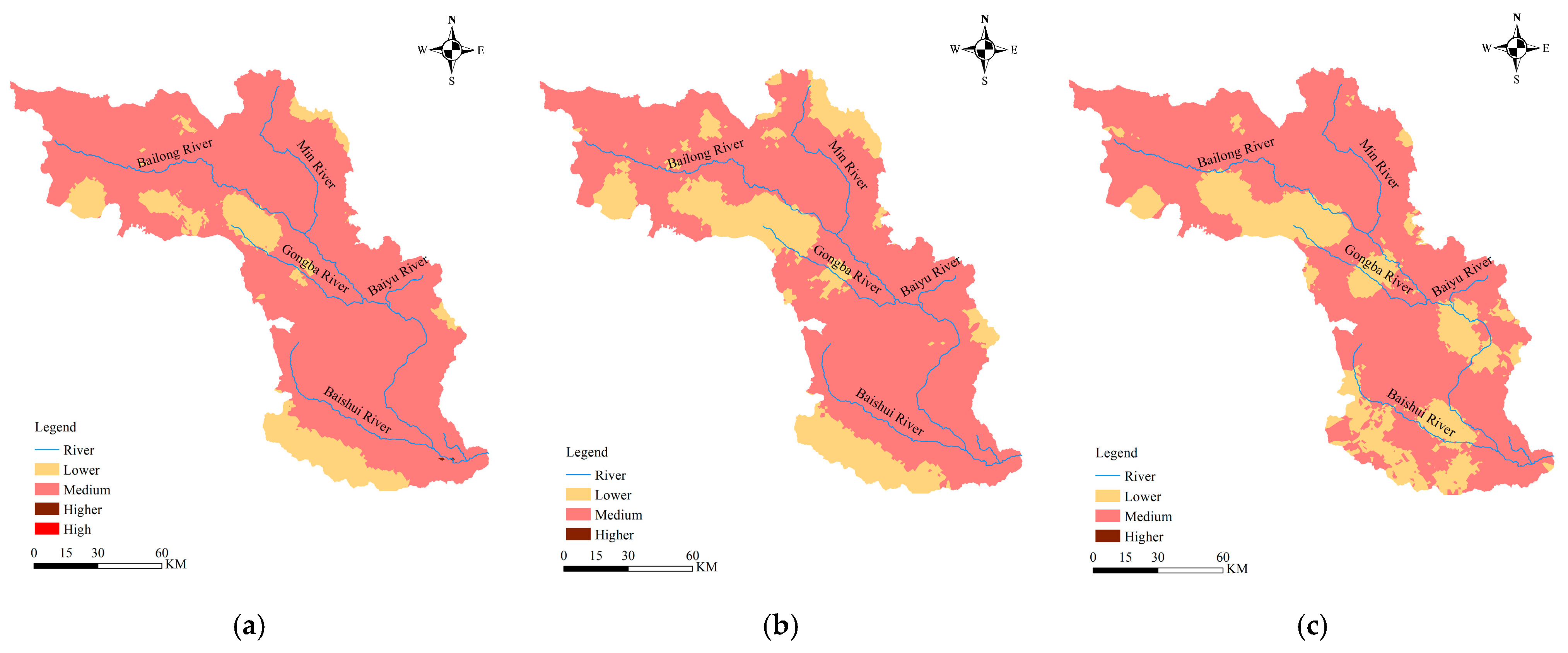
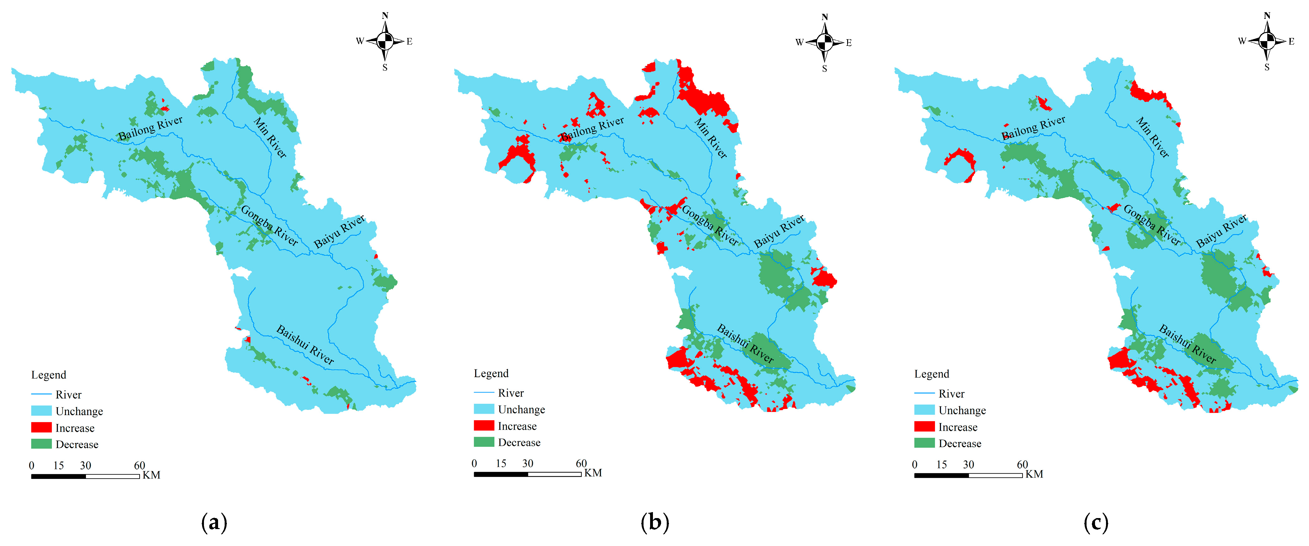
4.2. Analysis of Spatial and Temporal Changes in Landscape Ecological Risk

To reflect the distribution of LER in the basin, the study area was divided into low-risk areas [0–0.2), lower-risk areas [0.2–0.4), medium-risk areas [0.4–0.6), higher-risk areas [0.6–0.8), and high-risk areas [0.8–1] using the equal spacing method. The domains of the values of the LER indices of the three years were 0.34–0.81, 0.34–0.78, and 0.26–0.76. As can be seen from Figure 7, the value of LER in the basin continued to decline from 2000 to 2020, the area of the medium-risk zone was reduced, and the landscape ecology of the basin developed in a positive direction. On this time scale, the upper area of the Gongba River became a typical area of LER reduction during 2000–2010. The lower-risk area showed a development trend from point to point, forming a concentrated and large lower-risk area. Meanwhile, in the upper Min River, the area of the lower-risk areas increased, and the LER of the entire upper basin showed a noticeable trend of reduction. Between 2010 and 2020, the landscape ecological status of the middle and lower reaches of the basin improved. In the confluence area of the Baiyu River and the upper reaches of the Baishui River, the area of the lower-risk zone increased significantly, and it became a typical area of LER improvement in the basin. However, on the right bank of the Baishui River, the lower-risk zones were fragmented, and many new medium-risk zones were added. At the same time, on the left bank of the Min River, large areas of lower-risk areas were transformed into medium-risk areas, resulting in a significant increase in medium-risk areas. These areas showed ecological instability and increased LER in some areas. The distribution of LERs in the BRB is generally characterized by the point-like distribution of higher-risk zones, the centralized distribution of medium-risk zones, and the grouped distribution of lower-risk zones.

As can be seen in Figure 8, the northern and southern parts of the BRB belong to the main areas of increasing LER, and the southwestern and central parts belong to the main areas of decreasing LER. In 2000–2010, the LER of the basin was mainly in a decreasing trend, and from 2010 to 2020, the changes in LER of the basin were prominent, with areas of decreasing and increasing risk co-existing. The northeastern and southern parts were dominated by increasing risk, and a decreasing trend was observed in the LER in the Gongba River Basin, Baiyu River Basin, and Baishui River Basin. The overall risk changes in the study area are characterized by a prominent reduction, with some areas experiencing an increase.

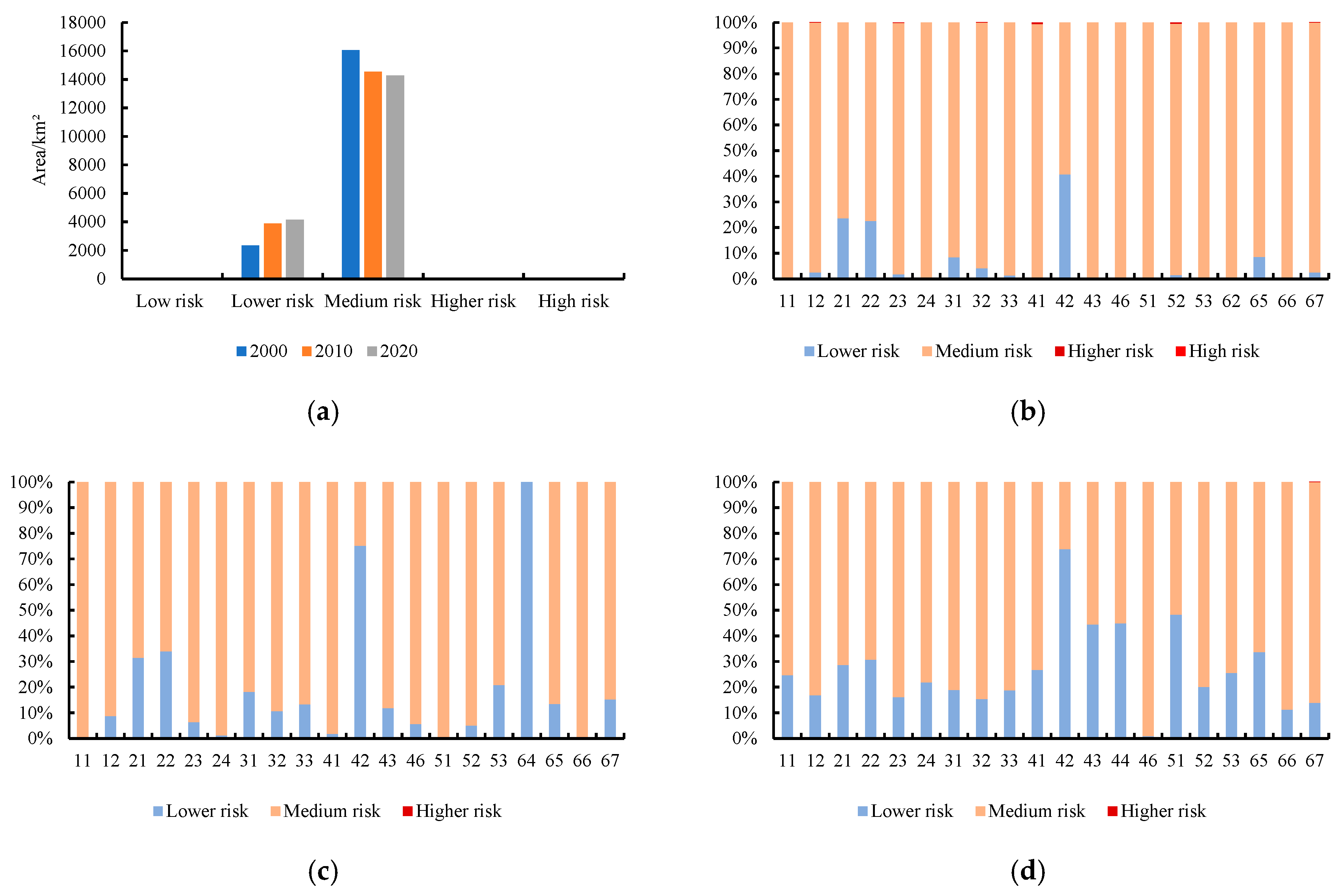
4.3. Landscape Ecological Risk Analyses for Different Site Types

The overall LER of the BRB is characterized by an increase in lower-risk zones and a decrease in medium-risk zones, as shown in Figure 9. In 2000, the lower-risk zone was dominated by forest land (21,22) and water bodies (42), with forest land dominated by natural forest land and artificial forest land (21) and shrubland (22), and water bodies dominated by lakes (42). By 2010, some grasslands (31,32,33), built-up land (52,53), and unused land (64,65,67) were added as lower-risk areas, further increasing the size of the lower-risk areas. By 2020, the area of lower-risk zones with all types of land was roughly 20 percent of the total area of that type of land, with the area of lower-risk zones on lakes (42), reservoirs (43), beach land (46), and urban land (51) exceeding 40 percent of the total area of the type. In 2000, natural forest land and artificial forest land (21), scrubland (22), and lakes were partly within lower-risk areas, influenced by the land use type. In 2010, all of the marsh land (64) was in the lower-risk area. Secondly, over 70 percent of the lake area (42) was in the lower-risk zone, but wet fields (11), rivers and canals (41), and bare rocky texture (66) were largely in the medium-risk zone. The LER did not change between 2000 and 2010. By 2020, there was an increase in the area of lower-risk zones for all land types except beach land (46). Notably, the proportion of lower-risk zone areas was greater for urban land (51) and other build-up land (53) than for rural residential areas (52). In the case of basin land, the proportion of lower-risk areas of lakes (42), reservoirs (43), and glacial and snow land (44) was consistently more significant than the area of rivers and canals (41).

4.4. Spatial Autocorrelation and Hotspot Analysis

4.4.1. Comparison of Evaluation Results of Multiple Weights

A global autocorrelation analysis was carried out to analyze the spatial clustering pattern of the LER evaluation results. The results are shown in

Table 4. The results of Global Moran’s I.

	Moran’s I Value	p Value	Z Value
2000	0.28	0.00	11.41
2010	0.25	0.00	10.17
2020	0.12	0.00	5.00

. The Moran’s I values were all greater than 0.1, the p-values were all less than 0.01, and the z-scores were all greater than 2.58, which indicated that the LER indices had significant a spatial differentiation and autocorrelation. Subsequently, local Moran index calculations were carried out to analyze the reasons for the clustering of high and low values in each risk grid.

As shown in Figure 10, the LISA clustering map contains four types of clusters: high–high (HH) clustering, low–low (LL) clustering, low–high (LH) clustering, and high–low (HL) clustering. The HH aggregation appears to increase and then decrease, and the LL aggregation appears to decrease continuously. Among them, the HL and LH grids as anomalous clustering spaces should be focused on for analysis. The anomalous clustering grid was 21 in 2000, 25 in 2010, and 44 in 2020. This demonstrates that the spatial clustering of LERs in the study area has gradually developed from simple HH and LL clustering to the coexistence of multiple clustering patterns. Among them, the Baishui River area and Gongba River area with LL aggregation have gradually evolved into HL aggregation areas. In addition, the LH distribution was scattered in the basin, mainly concentrated in the northern part. Overall, the LER of the basin gradually changed from the beginning of the HH and LL aggregation types to an aggregation pattern with HL and LL distributions as the main types. This reflects the transformation of LER in the BRB from a single aggregated distribution to a multi-scenario and multi-type combined distribution.

4.4.2. Hot Spot Analysis

Based on the clustering and outlier analysis, the specific clustering of the LER indices in space was explored using a hot spot analysis. As shown in Figure 11, the analysis of the LER hot spots revealed that the distribution of cold spots in the basin was evident from 2000 to 2010. The cold spot area was dominated by the 95% confidence interval area, mainly on the right bank of the Baishui River and the upstream area of the Gongba River. These are areas with dense vegetation cover and little artificial interference. The hot spot areas were mainly concentrated in the left bank of the Min River and the middle reaches of the Bailong River, which are areas with frequent human activities in the Bailong River valley zone. By 2020, the hot spot areas in the BRB were shifted, mainly distributed in the northwestern edge of the basin, and the rest of the hot spot areas were sporadically distributed in the basin. The cold spot areas were significantly reduced, and those on both sides of the Baishui River disappeared. In contrast, the cold spot area in the upper reaches of the Gongba River increased significantly in 2020. The changes in the distribution of cold spot areas in the study area as a whole reflect the increase in cold spot areas in the upstream area of the Gongba River, indicating that the Gongba River Basin’s LER is stable. However, the cold spot area in the Baishui River Basin decreased, and the LER showed an unstable state. In contrast, the hot spot area increased in the northwestern region located upstream of the Bailong River, reflecting that the clustering effect of the LER in this region also increased.

5. Discussion

5.1. Scale Dependence of Weight Assignment

The problem of scale has always been troubling and has always been a focus of research in geography, ecology, and other disciplines. Scale effects are cut across many fields of study, such as landscape patterns and processes, ecosystem structure and function, and topographic features [44]. In their study of LER in the Shandong Peninsula, Zhu et al. found that different scales had significant effects on the uncertainty of the evaluation results [45]. This paper is based on the calculation of empowerment results of different scales and different empowerment methods to solve the problem of empowerment methods and optimal scales in the evaluation of LER and to provide a theoretical basis for other LER studies. Although the evaluation of LER will be affected by different empowerment methods, the LER results will also show a changing trend when constructing the LER evaluation formula using the selected different empowerment methods. Choosing the method with the most significant results for most types of LER classes will be significant for us to determine the best empowerment method. In the past, in LER evaluations, research on the empowerment of landscape indices was conducted according to the Delphi method, which caused the LER evaluation to become a subjective judgement [8,24,25]. Previous researchers have also reached different conclusions in the same region based on different research scales [17,46], suggesting that inconsistencies in weighting methods and research scales may be an important reason for such results. This study confirms that the response relationship between different weighting methods and study scales is also inconsistent. The empowerment of weights to landscape indices is more affected by the grid scale, which means that the evaluation results of an LER are more likely to be affected by the study scale; a finding that is consistent with Chen et al. [47]. As shown in Figure 12, the PD index and SPLIT index weights using the coefficient of variation method will be higher than those of the entropy weight and game theory methods. Using the entropy weight method, the CONNECT index, SHDI index, and SHEI index will be much larger than the empowerment results of the coefficient of variation and game theory methods. By calculating the empowerment results of the landscape indices under different scales, the best empowerment method in the study of LER is determined by using the change of index weights, avoiding the influence of scale dependence on the evaluation results and solving the problem of selecting the empowerment method in the evaluation of LER.

5.2. Response Relationship between Land Use and Landscape Ecological Risk

Land use change is divided into natural succession and human intervention. As an important ecological barrier area in the upper reaches of the Yangtze River, the BRB has a predominantly forest land and grass land use type. During the study period, the area of dry cultivated land decreased the most, and the rural residential area increased the most. Some studies have found that reductions in arable land are favorable in reducing landscape ecological risk [48]. Combined with land use area changes, this study found that, along with urbanization, agricultural practitioners began to move to the cities. The area under agricultural cultivation was significantly reduced, thus reducing the LER in some areas of the BRB. The BRB is in the underdeveloped mountainous regions in the west, and due to economic and topographical conditions, the scale of urbanization in these areas is limited. Additionally, the land used for construction is more significant in rural residential areas than urban land. The unbalanced growth of construction land leads to a more noticeable increase in the LER in rural residential areas than in urban land.

Farmers can be protected from landscape risks through the sustainable development of agricultural landscapes [49]. Shi et al. showed that the increase in LER was due to urbanization construction in an overall study of LER in China [50], but the change in LER in the BRB was the opposite of such studies. The unique geographical conditions and lower level of economic development in the BRB have led to the construction of rural settlements being higher than that of urbanization, thus creating an increase in LER mainly in areas of rural settlements. With the change in natural succession, the alpine desert and tundra area in the basin shrank, and the ecological environment developed favorably. Some scholars studying the typical area of the Yellow River Basin found that with the gradual increase in the area of forest land and grasslands, the LER appeared to decrease [51]. In this paper, it was found that the area of forest land and grassland in the BRB gradually increased, which optimized the landscape pattern of the BRB to a certain extent and played a positive role in reducing the LER. This finding is consistent with the results of the ClujNapoca forest in Romania [52]. Of interest is the disappearance of the Gobi in the basin and the increase and then disappearance of marshes, which is a change in land use type and reflects the continued benign ecological development of the BRB. In general, the overall LER showed a decreasing development trend, indicating that the implementation of national policies and the transfer of industry types played a positive role in the ecological environment, which is consistent with the results of Liu et al.’s evaluation of LER in a county [53]. Some studies have pointed out that dealing with the remediation of abandoned land has positive significance for the improvement of the natural ecological environment [54], which is an important reference value for the sustainable development of the landscape in the BRB.

5.3. Spatial Characterization of Landscape Ecological Risk

The LER in the BRB showed a spatially clustered distribution [55]. With time, the HH and LL aggregation within the study area changed to HL and LL aggregation. The change in the aggregation type reflects the phenomenon of diffusion of LERs in the basin from the previous single aggregation to the current state of multi-region dispersion. The HH aggregation area in the Min River basin decreased over time, and LER was improved. Consistent with the results of Li et al.’s study of the Selenga River Basin [41], the HH aggregation appeared to have a trend of increasing and then decreasing, reflecting the improvement of regional LER. Some of the LL aggregation areas in the Baishui River Basin and Gongba River Basin were replaced by HL aggregation, indicating that the trend of increasing LER in this region must be paid attention to in future development and planning. In 2020, the BRB presented the spatial distribution characteristics of “HL dispersion, LL aggregation”. This indicates that the low-value area of the LER in the BRB decreased but maintained the aggregation characteristics as a whole. HL aggregation was scattered throughout the basin, indicating the risk of further spreading of ecological risk; a conclusion consistent with the findings of Zhou et al. [56]. Over time, the area of non-aggregated LER of the study area increased, which is consistent with the trend of the global Moran’s index decreasing, which is consistent with the trend of Cao et al. [57]. Overall, the dramatic shift in land use area in the BRB over the past 20 years has significantly impacted the LER’s spatial distribution characteristics [11].

5.4. Research Shortcomings and Prospects

Evaluating regional LER based on land use data is applicable to multi-scale regions and is a feasible methodology that is important for land use optimization and sustainable regional development [58]. As credible scientific results, the conclusions of this study can be directly used to support the decision-making process. In a broader context, such work benefits those seeking similar evaluations, especially when analyzing landscape indices in the context of scale effects, as it reduces assessment uncertainty through a novel approach. However, there are inevitably some shortcomings in this study.

Firstly, the influence of the granularity effect on the results of the landscape index is not considered in the calculation process of the landscape index. Combined with related studies [59], it was found that the spatial resolution difference of remote sensing images would also affect the results of the landscape index. Secondly, some scholars [60] have gradually introduced socio-economic data, climate data, and topographic data into LER evaluations. As ecological processes have complex dynamic characteristics and spatial heterogeneity, any scale will be affected by the interactions between social, economic, or decision-making factors at other scales. Therefore, the scale of LER often has significant uncertainty [61], which needs to be further explored in future research in combination with practice. However, due to the inconsistency between the concepts of such indicators and landscape indices, the weights of these indicators and how these indicators affect LER cannot be accurately determined. This series of questions is not accounted for, so such indicators are not used in this study for the time being and need to be further explored in future research in combination with practice. In addition, because of the characteristics of landscape indexes, the landscape indexes selected in this paper have a certain correlation between the indexes in the correlation analyses. Therefore, the evaluation results of the LER were disturbed by the correlation between the landscape indexes. However, this did not have a significant effect on the final evaluation results. Finally, due to the uniqueness of the land use and geomorphological types in the study area, this study did not involve mudflats, deserts, and saline soils. Therefore, the study’s conclusions cannot be widely applied to other study areas with different landscape characteristics. It is necessary to explore future study samples that include more land use types. These will be analyzed in further research work, but these factors are unlikely to influence the main conclusions of this study.

6. Conclusions

A landscape ecological risk assessment helps researchers to characterize landscape ecological security, which is key to landscape sustainability [62,63,64]. Under sustainable development and ecological environmental protection, this paper studies the mechanism of weight empowerment and LER evaluation in the BRB as an example. Different from the traditional evaluation methods, this study introduces the weight empowerment analysis into the LER evaluation and specifies the best empowerment method of the landscape index, providing a universal theoretical contribution. The main conclusions are as follows: (1) the entropy weighting method is the optimal empowerment method in the LER study. (2) Land use in the study area was dominated by forest land and grasslands. Cultivated land was the land use type with the most reduced area. The decrease in the area of cultivated land was the main factor leading to the decrease in the LER. (3) The LER showed an overall decreasing trend over time. Medium-risk areas decreased, and lower-risk areas increased. The upper Min River area is an important area for future ecological protection. (4) The global Moran’s I value in the study area gradually decreased, but the critical value was greater than 0.1. The LER was positively correlated in spatial distribution but had a dispersed trend. In the future, we need to be alert to the spatial transfer of LER. (5) The cold spot area in the Baishui River Basin is decreasing and the LER is unstable, so we need to strengthen protections in the future.

Based on the analysis of spatial and temporal changes in land use types and LER, the following recommendations are provided for the ecological, environmental protection, and sustainable development of the BRB: (1) in response to the phenomenon of decreasing cultivated land and increasing land use for rural residential area in the basin, corresponding policies should be formulated to guarantee the amount of minimum bare cultivated land to ensure the security of regional food supply. At the same time, the protection of abandoned cultivated land should be dealt with to realize the return of cultivated land to forest land and grasslands. The scale of rural self-built houses should be restricted to avoid the waste of cultured land resources and the escalation of LER. (2) Attention should be paid to the increased LER in the Baishui River Basin and the upper reaches of the Min River. In the future, these areas need to be focused on, and targeted management programs should be put forward to strengthen ecological environmental protection in response to the increase in LERs caused by different factors. (3) By analyzing the temporal and spatial changes of the LER in the basin and combining the changing characteristics of the landscape ecological environment, an early warning mechanism for LER is established. Establishing this early warning mechanism is conducive to preventing and resolving major ecological and environmental problems and maintaining the region’s sustainable development.

References

1. Gong, J.; Cao, E.; Xie, Y.; Xu, C.; Li, H.; Yan, L. Integrating ecosystem services and landscape ecological risk into adaptive management: Insights from a western mountain-basin area, China. J. Environ. Manag. 2021, 281, 111817. [Google Scholar] [CrossRef] [PubMed]
2. Gong, J.; Xie, Y.; Cao, E.; Huang, Q.; Li, H. Integration of InVEST-habitat quality model with landscape pattern indexes to assess mountain plant biodiversity change: A case study of Bailongjiang watershed in Gansu Province. J. Geogr. Sci. 2019, 29, 1193–1210. [Google Scholar] [CrossRef]
3. Gong, J.; Liu, D.; Gao, B. Tradeoffs and synergies of ecosystem services in western mountainous China: A case study of the Bailongjiang basin in Gansu, China. J. Appl. Ecol. 2020, 31, 1278–1288. [Google Scholar]
4. Wang, H.; Liu, X.; Zhao, C.; Chang, Y.; Liu, Y.; Zang, F. Spatial-temporal Pattern Analysis of Landscape Ecological Risk Assessment Based on Land use/Land Cover Change in Baishuijiang National Nature Reserve in Gansu Province, China. Ecol. Indic. 2021, 124, 107454. [Google Scholar] [CrossRef]
5. Tian, P.; Li, J.; Shi, X. Spatial and Temporal Change of Land Use Pattern and Ecological Risk Assessment in Zhejiang Province. Resour. Environ. Yangtze River Basin 2018, 27, 59–68. [Google Scholar]
6. Shi, P.; Qin, Y.; Li, P. Development of a landscape index to link landscape patterns to runoff and sediment. J. Mt. Sci. 2022, 19, 2905–2919. [Google Scholar] [CrossRef]
7. Peng, J.; Dang, W.; Liu, Y. Progress and Prospects of Landscape Ecological Risk Assessment Research. Acta Geogr. Sin. 2015, 70, 664–677. [Google Scholar]
8. Ai, J.; Yu, K.; Zeng, Z.; Yang, L.; Liu, Y.; Liu, J. Assessing the dynamic landscape ecological risk and its driving forces in an island city based on optimal spatial scales: Haitan Island, China. Ecol. Indic. 2022, 137, 108771. [Google Scholar] [CrossRef]
9. Cui, L.; Zhao, Y.; Liu, J. Landscape ecological risk assessment in Qinling Mountain. Geol. J. 2018, 53, 342–351. [Google Scholar] [CrossRef]
10. Chen, X.; Yang, Z.; Wang, T.; Han, F. Landscape Ecological Risk and Ecological Security Pattern Construction in World Natural Heritage Sites: A Case Study of Bayinbuluke, Xinjiang, China. ISPRS Int. J. Geo-Inf. 2022, 11, 6. [Google Scholar] [CrossRef]
11. Lin, X.; Wang, Z. Landscape Ecological Risk Assessment and Its Driving Factors of Multi-mountainous City. Ecol. Indic. 2023, 146, 109823. [Google Scholar] [CrossRef]
12. Asada, H.; Minagawa, T. Impact of Vegetation Differences on Shallow Landslides: A Case Study in Aso, Japan. Water 2023, 15, 18. [Google Scholar] [CrossRef]
13. Zhang, H.; Zhang, J.; Lv, Z.; Yao, L.; Zhang, N.; Zhang, Q. Spatio-Temporal Assessment of Landscape Ecological Risk and Associated Drivers: A Case Study of the Yellow River Basin in Inner Mongolia. Land 2023, 12, 1114. [Google Scholar] [CrossRef]
14. Wang, W.; Wang, H.; Zhou, X. Ecological risk assessment of watershed economic zones on the landscape scale: A case study of the Yangtze River Economic Belt in China. Reg. Environ. Chang. 2023, 23, 105. [Google Scholar] [CrossRef]
15. Liu, D.; Chen, H.; Zhang, H.; Geng, T.; Shi, Q. Spatiotemporal Evolution of Landscape Ecological Risk Based on Geomorphological Regionalization during 1980–2017: A Case Study of Shaanxi Province, China. Sustainability 2020, 12, 941. [Google Scholar] [CrossRef]
16. Wang, S.; Tan, X.; Fan, F. Landscape Ecological Risk Assessment and Impact Factor Analysis of the Qinghai–Tibetan Plateau. Remote Sens. 2022, 14, 4726. [Google Scholar] [CrossRef]
17. Lan, Y.; Chen, J.; Yang, Y.; Ling, M.; You, H.; Han, X. Landscape Pattern and Ecological Risk Assessment in Guilin Based on Land Use Change. Int. J. Environ. Res. Public Health 2023, 20, 2045. [Google Scholar] [CrossRef] [PubMed]
18. Tan, R.; Zhou, K. Examining the Causal Effects of Road Networks on Landscape Ecological Risk: The Case of Wuhan, China. J. Urban Plan. Dev. 2023, 149, 2. [Google Scholar] [CrossRef]
19. Yan, Z.; You, N.; Wang, L.; Lan, C. Assessing the Impact of Road Network on Urban Landscape Ecological Risk Based on Corridor Cutting Degree Model in Fuzhou, China. Sustainability 2023, 15, 1724. [Google Scholar] [CrossRef]
20. Zhou, Z.; Zhao, W.; Lv, S.; Huang, D.; Zhao, Z.; Sun, Y. Spatiotemporal Transfer of Source-Sink Landscape Ecological Risk in a Karst Lake Watershed Based on Sub-Watersheds. Land 2023, 12, 1330. [Google Scholar] [CrossRef]
21. Zhao, L.; Shi, Z.; He, G.; He, L.; Xi, W.; Jiang, Q. Land Use Change and Landscape Ecological Risk Assessment Based on Terrain Gradients in Yuanmou Basin. Land 2023, 12, 1759. [Google Scholar] [CrossRef]
22. Peng, J.; Zong, M.; Hu, Y.; Liu, Y.; Wu, J. Assessing Landscape Ecological Risk in a Mining City: A Case Study in Liaoyuan City, China. Sustainability 2015, 7, 8312–8334. [Google Scholar] [CrossRef]
23. Li, C.; Zhang, J.; Philbin, S.; Yang, X.; Dong, Z.; Hong, J.; Ballesteros-Pérez, P. Evaluating the impact of highway construction projects on landscape ecological risks in high altitude plateaus. Sci. Rep. 2020, 12, 5107. [Google Scholar] [CrossRef] [PubMed]
24. Chen, L.; Ma, Y. Ecological Risk Identification and Ecological Security Pattern Construction of Productive Wetland Landscape. Water Resour Manag. 2023, 37, 4709–4731. [Google Scholar] [CrossRef]
25. Wang, Q.; Zhang, P.; Chang, Y.; Li, G.; Chen, Z.; Zhang, X.; Xing, G.; Lu, R.; Li, M.; Zhou, Z. Landscape pattern evolution and ecological risk assessment of the Yellow River Basin based on optimal scale. Ecol. Indic. 2024, 158, 111381. [Google Scholar] [CrossRef]
26. Li, B.; Yang, Y.; Jiao, L.; Yang, M.; Li, T. Selecting ecologically appropriate scales to assess landscape ecological risk in megacity Beijing, China. Ecol. Indic. 2023, 154, 110780. [Google Scholar] [CrossRef]
27. Xu, W.; Wang, J.; Zhang, M.; Li, S. Construction of landscape ecological network based on landscape ecological risk assessment in a large-scale opencast coal mine area. J. Clean. Prod. 2021, 286, 125523. [Google Scholar] [CrossRef]
28. Aksu, G.; Musaoglu, N.; Uzun, A. Ecological risk analysis based on analytic hierrchy process. Fresenius Environ. Bull. 2017, 26, 84–92. [Google Scholar]
29. Zhu, C.; Fang, C.; Zhang, L. Analysis of the coupling coordinated development of the Population-Water-Ecology-Economy system in urban agglomerations and obstacle factors discrimination: A case study of the Tianshan North Slope Urban Agglomeration, China. Sustain. Cities Soc. 2023, 90, 104359. [Google Scholar] [CrossRef]
30. Algayer, B.; Wang, B.; Bourennane, H.; Zheng, F.; Duval, O.; Li, G.; Le Bissonnais, Y.; Darboux, F. Aggregate stability of a crusted soil: Differences between crust and sub-crust material, and consequences for interrill erodibility assessment. An example from the Loess Plateau of China. Eur. J. Soil Sci. 2014, 65, 325–335. [Google Scholar] [CrossRef]
31. Wang, X.; Che, Q.; Wang, L.; Li, G.; Sun, H.; Qin, W.; Chen, S.; Yao, S.; Meng, L.; Yu, X. Spatial–temporal pattern of urban ecological construction in the Yellow River basin and its optimization and promotion paths. Environ. Inform. Remote Sens. 2023, 11, 1147619. [Google Scholar]
32. Long, C.; Pang, Y.; Wang, Z. Study of the Sustainability of a Forest Road Network Using GIS-MCE. Forests 2023, 14, 2410. [Google Scholar] [CrossRef]
33. Zhao, L.; Ma, R.; Yang, Z.; Ning, K.; Chen, P.; Wu, J. Ecosystem health risk assessment of lakes in the Inner Mongolian Plateau based on the coupled AHP-SOM-CGT model. Ecol. Indic. 2023, 156, 111168. [Google Scholar] [CrossRef]
34. Peng, J.; Zhao, H.; Liu, Y.; Wu, J. Progress and Prospects of Research on the Construction of Regional Ecological Security Patterns. Geogr. Res. 2017, 36, 407–419. [Google Scholar]
35. Li, Q.; Ma, B.; Zhao, L.; Mao, Z.; Luo, L.; Liu, X. Landscape Ecological Risk Evaluation Study under Multi-Scale Grids—A Case Study of Bailong River Basin in Gansu Province, China. Water 2023, 15, 3777. [Google Scholar] [CrossRef]
36. Chen, M.; Lu, D.; Zhang, H. Comprehensice Evaluation and the Driving Factors of China’s Urbanization. Acta Geogr. Sin. 2009, 64, 387–398+6. [Google Scholar]
37. Chen, S.; Zou, Q.; Wang, B.; Zhou, W.; Yang, T.; Jiang, H.; Zhou, B.; Yao, H. Disaster risk management of debris flow based on time-series contribution mechanism (CRMCD): Nonnegligible ecological vulnerable multi-ethnic communities. Ecol. Indic. 2023, 157, 111266. [Google Scholar] [CrossRef]
38. Xu, N.; Hu, X.; Wang, X.; Liu, Z.; Tian, J.; Ren, Z. Spatiotemporal variations of eco-environmental vulnerability in Shiyang River Basin, China. Ecol. Indic. 2024, 158, 111327. [Google Scholar] [CrossRef]
39. Yang, X.; Shen, J. Landscape Sensitivity Assessment of Historic Districts Using a GIS-Based Method: A Case Study of Beishan Street in Hangzhou, China. ISPRS Int. J. Geo-Inf. 2023, 12, 462. [Google Scholar] [CrossRef]
40. Niu, S.; Li, G.; Zhang, S. Driving Risk Assessment Model of Commercial Drivers Based on Satellite positioning Data. China J. Highw. Transp. 2020, 33, 202–211. [Google Scholar]
41. Li, W.; Lin, Q.; Hao, J.; Wu, X.; Zhou, Z.; Lou, P.; Liu, Y. Landscape Ecological Risk Assessment and Analysis of Influencing Factors in Selenga River Basin. Remote Sens. 2023, 15, 4262. [Google Scholar] [CrossRef]
42. Ma, J.; Khromykh, V.; Wang, J.; Zhang, J.; Li, W.; Zhong, X. A landscape-based ecological hazard evaluation and characterization of influencing factors in Laos. Environ. Inform. Remote Sens. 2023, 11, 1276239. [Google Scholar] [CrossRef]
43. Zhang, X.; Dong, X.; Xu, C.; Wang, R.; Lv, T.; Ranagalage, M. Landscape Ecological Risk Assessment in the Dongjiangyuan Region, China, from 1985 to 2020 Using Geospatial Techniques. Geomat. Nat. Hazards Risk 2023, 14, 2173662. [Google Scholar] [CrossRef]
44. Gibson, C.C.; Ostrom, E.; Ahn, T.-K. The concept of scale and the human dimensions of global change: A survey. Ecol. Econ. 2000, 32, 217–239. [Google Scholar] [CrossRef]
45. Ju, H.; Niu, C.; Zhang, S.; Jiang, W.; Zhang, Z.; Zhang, X.; Yang, Z.; Cui, Y. Spatiotemporal patterns and modifiable areal unit problems of the landscape ecological risk in coastal areas: A case study of the Shandong Peninsula, China. J. Clean. Prod. 2021, 310, 127522. [Google Scholar] [CrossRef]
46. Yang, Y.; Chen, J.; Lan, Y.; Zhou, G.; You, H.; Han, X.; Wang, Y.; Shi, X. Landscape Pattern and Ecological Risk Assessment in Guangxi Based on Land Use Change. Int. J. Environ. Res. Public Health 2022, 19, 1595. [Google Scholar] [CrossRef]
47. Chen, J.; Yang, Y.; Feng, Z.; Huang, R.; Zhou, G.; You, H.; Han, X. Ecological Risk Assessment and Prediction Based on Scale Optimization—A Case Study of Nanning, a Landscape Garden City in China. Remote Sens. 2023, 15, 1304. [Google Scholar] [CrossRef]
48. Zhu, Y.; Hou, Z.; Xu, C.; Gong, J. Ecological Risk Identification and Management Based on Ecosystem Service Supply and Demand Relationship in the Bailongjiang River Watershed of Gansu Province. Sci. Geogr. Sin. 2023, 43, 423–433. [Google Scholar]
49. Kumaraswamy, S.; Kunte, K. Integrating biodiversity and conservation with modern agricultural landscapes. Biodivers. Conserv. 2013, 22, 2735–2750. [Google Scholar] [CrossRef]
50. Shi, Y.; Feng, C.; Yu, Q.; Han, R.; Guo, L. Contradiction or coordination? The spatiotemporal relationship between landscape ecological risks and urbanization from coupling perspectives in China. J. Clean. Prod. 2022, 363, 132557. [Google Scholar] [CrossRef]
51. Qu, Y.; Zong, H.; Su, D.; Ping, Z.; Guan, M. Land Use Change and Its Impact on Landscape Ecological Risk in Typical Areas of the Yellow River Basin in China. Int. J. Environ. Res. Public Health 2021, 18, 11301. [Google Scholar] [CrossRef]
52. Sestras, P.; Bondrea, M.V.; Cetean, H.I.; SĂLĂGean, T.; BilaŞCo, Ş.; Sanda, N.A. Ameliorative, ecological and landscape roles of Făget Forest, Cluj-Napoca, Romania, and possibilities of avoiding risks based on GIS landslide susceptibility map. Not. Bot. Horti Agrobot. Cluj-Napoca 2018, 46, 292–300. [Google Scholar] [CrossRef]
53. Liu, J.; Wang, M.; Yang, L. Assessing Landscape Ecological Risk Induced by Land-Use/Cover Change in a County in China: A GIS and Landscape-Metric-Based Approach. Sustainability 2020, 12, 9037. [Google Scholar] [CrossRef]
54. Hu, J.; Liu, Y.; Dai, Q.; Yang, B.; Zhou, W. Evaluation of ecotourism suitability based on AHP-GIS: Taking Xiaoxiangling area of the Giant Panada National Park and the Surrounding communities as an example. Chin. J. Appl. Ecol. 2024, 1–11. [Google Scholar] [CrossRef]
55. Gong, J.; Gao, J.; Zhang, L.; Xie, Y.; Zhao, C.; Qian, D. Distribution Characteristics of Ecological Risks in Land-use Based on Terrain Gradient and Landscape Structure: Taking Bailongjiang Watershed as an Example. J. Lanzhou Univ. (Nat. Sci.) 2014, 50, 692–698. [Google Scholar]
56. Zhou, W.; Luo, J. Spatial-temporal Evolution of Ecosystem Service Value and Landscape Ecological Risk in Dry Valleys. Yangtze River 2023, 54, 85–93. [Google Scholar]
57. Cao, Y.; Dong, B.; Xu, H.; Xu, Z.; Wei, Z.; Lu, Z.; Liu, X. Landscape Ecological Risk Assessment of Chongming Dongtan Wetland in Shanghai from 1990 to 2020. Environ. Res. Commun. 2023, 5, 105016. [Google Scholar] [CrossRef]
58. Wang, D.; Ji, X.; Li, C.; Gong, Y. Spatiotemporal Variations of Landscape Ecological Risks in a Resource-Based City under Transformation. Sustainability 2021, 13, 5297. [Google Scholar] [CrossRef]
59. Bai, Y.; Liao, S.; Sun, J. Scale effect and methods for accuracy evaluation of attribute information loss in rasterization. J. Geogr. Sci. 2011, 21, 1089–1100. [Google Scholar] [CrossRef]
60. Molinos, J.; Takao, S.; Kumagai, N.; Poloczanska, E.; Burows, M.; Fujii, M.; Yamano, H. Improving the interpretability of climate landscape metrics: An ecological risk analysis of Japan’s Marine Protected Areas. Glob. Chang. Biol. 2017, 23, 4440–4452. [Google Scholar] [CrossRef]
61. Fu, B.; Lu, Y. The progress and perspectives of landscape ecology in China. Prog. Phys. Geogr. 2006, 30, 232–244. [Google Scholar] [CrossRef]
62. Gao, Y.; Wu, Z.F.; Lou, Q.S.; Huang, H.M.; Cheng, J.; Chen, Z.L. Landscape ecological security assessment based on projection pursuit in Pearl River Delta. Environ. Monit. Assess. 2012, 184, 2307–2319. [Google Scholar] [CrossRef] [PubMed]
63. Zhou, K.H.; Liu, Y.L.; Tan, R.H.; Song, Y. Urban dynamics, landscape ecological security, and policy implications: A case study from the Wuhan area of central China. Cities 2014, 41, 141–153. [Google Scholar] [CrossRef]
64. Cen, X.T.; Wu, C.F.; Xing, X.S.; Fang, M.; Garang, Z.M.; Wu, Y.Z. Coupling Intensive Land Use and Landscape Ecological Security for Urban Sustainability: An Integrated Socioeconomic Data and Spatial Metrics Analysis in Hangzhou City. Sustainability 2015, 7, 1459–1482. [Google Scholar] [CrossRef]
Figure 1. Overview of the study area: (a) geographic location of the study area; (b) extracted watersheds based on DEM in the Bailong River.
Sustainability 16 01915 g001
Figure 2. Flow chart of this study.
Sustainability 16 01915 g002
Figure 3. Changes in weights under different methods and grid scales: (a) entropy weight method; (b) coefficient of variation method; (c) CRITIC; (d) independence rights coefficient method.
Sustainability 16 01915 g003
Figure 4. Changes in weights at different scales: (a) 1 km; (b) 2 km; (c) 3 km; (d) 4 km; (e) 5 km; and (f) 6 km.
Sustainability 16 01915 g004
Figure 5. Spatial distribution of LER using different approaches: (a) coefficient of variation method; (b) game theory; (c) entropy weight method.
Sustainability 16 01915 g005
Figure 6. Land use distribution maps: (a) 2000; (b) 2010; (c) 2020.
Sustainability 16 01915 g006
Figure 7. Spatial distribution of LER: (a) 2000; (b) 2010; (c) 2020.
Sustainability 16 01915 g007
Figure 8. Spatial transfer of LER: (a) 2000–2010; (b) 2010–2020; (c) 2000–2020.
Sustainability 16 01915 g008
Figure 9. Ratio of LER distribution across land use types: (a) 2000–2020; (b) 2000; (c) 2010; (d) 2020.
Sustainability 16 01915 g009
Figure 10. Local indicators of spatial autocorrelation clustering map (LISA) cluster map: (a) 2000; (b) 2010; (c) 2020.
Sustainability 16 01915 g010
Figure 11. Spatial distribution of hot spots and cold spots: (a) 2000; (b) 2010; (c) 2020.
Sustainability 16 01915 g011
Figure 12. Radar plot of weighting results of multiple methods for different landscape indices.
Sustainability 16 01915 g012