Abstract
The traffic flow parameters of the road network are most often evaluated through volumes, which are compared with its maximum volume (capacity) or speed and density. Capacity assessment was performed, considering horizontal and vertical orientation and characteristics of the traffic stream. This article presents the results of research on the identification of different states of creating congestion groups and their relationship to road capacity or decrease in speed. The following hypothesis was verified: when the capacity of the road is exceeded or almost reached, there is “always” a significant drop in the flow of traffic compared to when the capacity is not exceeded. The analysis showed that the average travel speed drops by 30% for the condition where groups of 25 or more vehicles are formed with a time interval of up to 4 s. The results make it possible to set traffic models in short time intervals according to real spatial conditions and to use them in the analysis of the environmental and safety impacts of road transport.
1. Introduction
Transport planning is generally concerned with the evaluation, assessment, design, and location of transport facilities and is based on specific transport planning models. Issues that require special consideration or are identified during the implementation of a solution require potential alternatives to be evaluated while considering the available budget.
Traffic flow monitoring [1,2,3] provides time-sorted data describing the current traffic situation on the road. The fundamental relationships of intensity, speed, and density are used in the assessment. In traffic engineering tasks, we often encounter the influence of ambient conditions of the alignment and the location of the route, which affect the traffic flow [4,5]. Computational algorithms incorporate them through various attributes such as curvature [6,7] and grade of climb/descent. The objectives of this paper are to present a detailed analysis of traffic groups on specific road network sections as a function of speed. The outputs are then used in setting up traffic models. Transport planning tasks are shifting from a purely technical analysis, including environmental aspects [8,9,10] and sustainability, toward a more integrated transport framework. The latter also includes psychological aspects of driver behavior [11] and their overall impact on driving.
Monitoring the flow of traffic in the territory contributes to the development of several disciplines. In addition to the basic traffic-engineering point of view, the parameterization of traffic conditions is beneficial, for example, in services (travel time), in the automotive industry (autonomous vehicles), and in other areas to make the supply and demand system more efficient. Research into the detection and categorization of congestion groups contributes to the creation of the structure of databases usable in the parameterization of traffic models or the development of AI solutions. The targeted intention is traffic management based on local conditions in the territory. The specific research was part of an extensive assignment of the Ministry of Transport of the Slovak Republic, and there are applications in international projects that are focused on mobility and reducing emission impacts.
Traffic flow theory studies the dynamic characteristics of traffic on road sections. Dynamic traffic flow models date back to the 1950s. In them, traffic is represented based on an analogy with water flows in rivers. These approaches allow us to treat individual vehicles as a “continuous fluid”. On this basis, macroscopic traffic flow theory focuses on variables that characterize the dynamic aspects of traffic (vehicle) movement:
- Vehicle density (k);
- Vehicle intensity (q);
- The average speed of vehicles (u).
Where a more in-depth traffic analysis is required, a more in-depth traffic flow study is necessary to relate the density, volume, and speed of the traffic flow to local conditions. Traffic models are a common tool for such analysis.
Macroscopic traffic models simply capture the general relationships between intensity, density, and speed. These relationships are expressed through drag functions. Volume-delay functions (VDFs) are mathematical relationships used by the traffic allocation step of demand forecasting models to take into account the effect of increased traffic flow on the time spent traveling each possible route between different travel sources and destinations [12]. The models abstract traffic into traffic flows that pass along traffic routes. These flows are often represented as a continuous flow and use formulations from hydrodynamic flow theories. The advantage of the macroscopic modeling approach is its simplicity and the ability to solve the equations of the traffic model according to the rules of network theory, while analytical solutions are possible. However, when dynamic variation of resistance and network segments is required, it is often necessary to use numerical solutions. However, a shortcoming of these models is that traffic flows are based on statistical data, which means that the model cannot provide detailed information about individual traffic events or entities (vehicles and drivers) [11].
Microscopic transport models, on the other hand, are designed to capture the detailed behavior of individual entities. These models focus on extreme detail, including capturing interactions between vehicles, the dynamics of lane changes, and intersection behavior. In this way, they provide complex information that is beyond the reach of macroscopic models. Microscopic models produce accurate descriptions of individual road users and therefore allow sophisticated behavioural strategies to be developed for each entity within the simulation. The main drawback of the microscopic approach is the considerable time-consuming nature of the simulation due to the number of entities and the number of interactions that the model has to manage. Another significant disadvantage is the need to correctly set the parameters of microscopic models, which requires the characteristics of each entity within the model to be defined consistently, completely, and consistently, thus requiring a huge amount of input data [11] with the required accuracy.
The traffic flow characteristics, such as the traffic volumes and the density, are estimated by averaging the vectors together in space and time [13]. The density is an indication of the freedom of movement of the users. The density is defined as the number of vehicles per unit length of the roadway. It is an essential traffic condition metric used in many traffic information systems [14]. The traffic volume is defined as the rate at which vehicles travel through a particular point or highway segment. Speed is measured in units of distance per unit of time, typically per hour [15]. The main attributes of the traffic flow are defined at each point in space and time, which means that the discrete nature of the traffic is mapped onto continuous variables. The change in time of these state variables can be modeled by partial differential equations (PDEs) consisting of the conservation of mass (vehicles) and the experimental relationship between intensity q and density k. This is referred to as the fundamental relationship of traffic flow theory and expresses that intensity q equals density k multiplied by speed u [11]:
Intensity is expressed in vehicles per hour. The maximum possible intensity of a road is called its capacity. The capacity of a road depends on the actual composition of vehicles and the nature of the road, but for motorways, we can consider a value of between 1800 and 2400 vehicles per hour for a single lane.
As the intensity increases, the distances between vehicles decrease, and they begin to interact with each other. At some point, the intensity reaches a maximum value (this is determined by the average speed of the traffic flow and its density). Since this maximum intensity is equal to the capacity of the road, it is called the capacity intensity and is denoted qc, qcap, or qama. The average time headway between vehicles is minimal at the state of maximum capacity, which is indicated by the formation of (local) clusters of vehicles (platoons). The maximum intensity (qmax) corresponds to the capacity speed, referred to as uc, ucap, or um. The capacity speed is below the maximum free flow speed uf. If some of the vehicles are following vehicles with dangerously small gaps (tailgating), such clusters of vehicles are very unstable. Whenever a vehicle in such a chain slows down a little, it can have a cascading effect that leads to aggressive braking of the following vehicles. Therefore, these maneuvers can violate the local capacity-flow condition and can translate into multiple collisions, making the traffic unstable [16].
Jammed traffic or stop-and-go traffic (traffic characterized by frequent stopping and starting) occurs after a state of capacity is reached, when vehicles continue to arrive, density increases, and the traffic flow becomes very unstable. In such a highly saturated traffic flow, hard braking of a vehicle may trigger a chain reaction that causes localized disruption of the flow up to a total breakdown of the flow. The density at which the traffic flow breaks down is called the critical density, kc, kcrit, or km (for a typical motorway, it is around 25 vehicles per km for a single lane) [10]. The optimal travel speed for a traffic stream can be calculated as um = qmax/km = 2000 ÷ 25 ≈ 85 km/h. When traffic stops, the spacing between vehicles reaches a minimum; thus, intensity and speed decrease to zero. This extreme condition can be called jammed traffic. The density of the traffic flow characteristic of this condition is called the jam density and is denoted as kj, kjam, or kmax. For a typical motorway, it is around 140 vehicles per kilometer for a single lane [16,17].
2. Methods of Processing and Evaluation of Data
Implementing real traffic flow characteristics into the assessment process is often very challenging. Dynamic effects and impacts of different variables oftentimes fundamentally affect the flow of the traffic stream. External influences may be low visibility, difficult directional or elevation guidance, poor road surfaces, etc. [18]. The classical capacity assessment of a two-lane road includes directional guidance through the proportion of angle change and length, elevation guidance through the determination of grade class, the proportion of trucks and slow vehicles, and the proportion of the route with no overtaking. In our traffic analysis, an analytical tool was developed to observe groups of vehicles on segments concerning intensity, density, and speed. The rationale for this activity was the need to refine the microscopic models to represent real road conditions more faithfully.
All surveys were conducted using automatic traffic counters (ATCs), which are defined as traffic survey devices. The function of ATCs is to create records of the progress of permanently conducted traffic surveys for further traffic engineering purposes [19].
Spot traffic surveys were conducted using the Sierzega SR4 microwave radar (Figure 1). This is an FMCW-based radar operating at 24 GHz at temperatures ranging from −25 °C to 60 °C. This radar is capable of recording vehicle speed with an accuracy of ±3%, in the range from 2 km/h to 255 km/h. It records the length of the vehicle to within ±20% decimeters, the time separation from the preceding vehicle to within ±0.2 s, and the passing time.
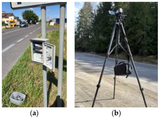
Figure 1.
Traffic data collection equipment: (a) Microwave radar, Sierzega SR4; (b) Sony digital camera with telescopic tripod and external power supply.
In the first phase of the analysis, radar data were collected from 60 profiles on regional, rural, and urban roads and a special subcategory of mountain passes. The profile or cross-section indicates the place where the measuring device was installed. In the study, we focused on the characteristics of the traffic flow during working days. During the working week, the share of freight traffic is increased. During the weekend, the intensity of holiday traffic is particularly important.
Basic characteristic data from the records were evaluated and later used to select profiles for deeper analysis. The Table 1 presents the average and maximum values of the traffic survey parameters for the given time intervals. The data represent the average of the measurements for the given road types and width ratios; maximum speeds were similar in the given categories. Regional roads had a design maximum speed of 90 km/h, and rural roads most often were close to towns or between two villages, where the design speed was 70 km/h. In urban environments, the maximum speed was 50 km/h. Mountain crossings are represented by two sections with a design speed of 90 km/h.

Table 1.
Average traffic load values at different time intervals for selected road types.
Traffic data were collected on profiles that were located outside important intersections or sections with a temporary change of organization. The radars were always installed in April, May, June, September, October, and November. After installing the measuring equipment, we conducted a short-term survey for the calibration setting of the vehicle type determination. As a rule, the measurement was processed within one week. The evaluation methodology was processed in successive steps. Saturated or most loaded time windows were selected from the course of the total load. Data were aggregated into 15 and 5 min groups.
The aspect of horizontal and vertical geometry was considered, especially when choosing the location of the profile survey and survey on the section. When calculating the capacity of the road, factors such as the curve angle, grade of climb, and the proportion of solid lines on the road were included in the calculation, according to Slovak regulations. The last factor characterizes the visibility. The data are freely available in the road network manager’s database. We compared the data from the road administrator with the results of the works [7,20], where the degradation of the road was monitored from the point of view of skidding. The same approach was taken when evaluating the road surface. Surface properties were evaluated and geolocated in the administrator’s database. From the database, we selected sections that reach average life parameters. In the current evaluation, this effect appears to be significant, especially on mountain passes. This issue will be examined in more detail in the next part of the research.
The different share of freight traffic and daily volumes are mainly based on the category of the roads in question. Regional and rural roads are burdened by a large share of transit traffic. This fact is known from the solution of the Transport Plan of the Žilina Region [21]. On both types of roads, high peak-hour traffic was observed. Urban roads were targeted in the area with a view to the city’s internal traffic and a significant share of public transport vehicles.
Table 1 shows that it is clear that urban roads experience the least load. The largest number of vehicles was recorded on rural roads. With a larger sample, the various states that occur here during the measurement are better analyzed. Mountain sections have an increased share of freight traffic, and, especially in winter, it is therefore necessary to detect and manage congestion in advance.
It is well known that the travel times of a road segment can vary significantly across different flow classes. The travel time plays an important role in the traveler’s route choice, departure time choice, and modal choice in the network [22,23,24]. Based on the average results, characteristic profiles were selected for which a specific evaluation of platoon frequencies concerning intensity was performed. Platoon has a negative impact on traffic performance because it increases travel time and air pollution [25]. This paper constructed a vehicle group monitoring model based on the time gap. The radar record was processed by indexing vehicles based on the time gap of consecutive vehicles. Platoons were then identified. A platoon consists of consecutive vehicles with a time gap of less than 2 s, 3 s, 4 s, and 5 s. By applying the time condition, the index of the group in the traffic stream was determined. Subsequent filtering of the data was used to evaluate the group occurrence, average speed, and probability distribution of group occurrence concerning local conditions.
The specific analysis was used to determine the cumulative probability for the occurrence of a given group in combination with intensity and speed. The graphical evaluation of congestion group formation was evaluated through a three-axis plot, where the x-axis represents the congestion group number according to the actual number of vehicles, the y-axis represents the ordered values in 15 min intensities from the lowest to the highest value, and the z-axis is represented through a graphical spectrum of the 85th percentile of speed occurrence (Figure 2a). Subsequently, the vehicle frequency indexations of the groups for the profile were evaluated (Figure 2b).
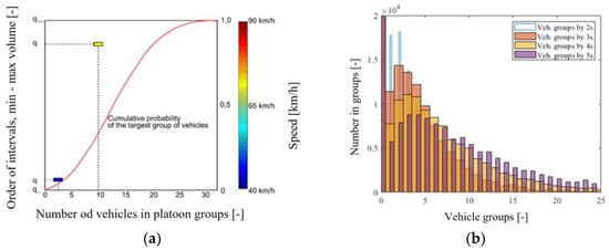
Figure 2.
Example of a graphical evaluation of the rate and formation of platoons at a given intensity: (a) Speed matrix of the 15 min volumes presented with vehicles groups ratio; (b) Number of vehicles in groups divided by time.
After developing an analytical tool to evaluate groups of vehicles, we focused on specific traffic surveys of road segments. The objective was to observe the number, type, and formation of vehicle groups under different edge conditions. We focused on the congested section between Žilina and Martin on the I/18 road. This section is notoriously known in Slovakia for frequent traffic problems. These issues are mainly caused by high traffic intensity. Annual average daily traffic (AADT) in this section is slightly below the value of 30,000 veh/24 h. Figure 3 presents the development of the traffic load on the analysed section.
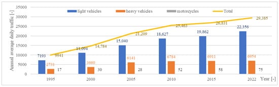
Figure 3.
Time report of annual average daily traffic (AADT).
The selected section is specific in several respects. The high traffic load values for a two-lane road have a relatively high proportion of trucks. On average, this is a 22% share. The reason for this is the location of the road and the traffic connection between the town of Žilina and the town of Martin. The Slovak Republic does not have a motorway link between the two largest cities (Bratislava—Košice). A motorway tunnel is currently being built in the section in question. After its opening, a significant increase in induced traffic is expected. According to [21], a total intensity of around 45,000 veh/24 h is expected. Another specific point is the design of the layout of the area. In 2009, a non-traditional, temporary solution with 2 + 1 lanes was proposed. The main reason for the change was to reduce traffic accidents. However, the steady increase in traffic caused such a solution to significantly disturb the homogeneity of vehicle travel speeds.
Figure 4 shows the location and designation of the monitored sections. Section 2 was further addressed in the study. The section in question was subjected to profile traffic surveys as well as surveys on individual sections of the road. Profile surveys were conducted from 29 June to 13 July 2022 with radar at four locations. The survey for the travel time study (segment surveys) was processed during the morning peak period of 06:00–10:00 a.m. and the afternoon peak period of 1:00–4:00 p.m. Vehicle group data were evaluated with regard to vehicle overtaking, travel times, etc.
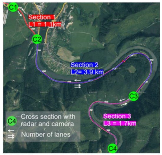
Figure 4.
Location of measured sections (road I/18).
3. Results
The first part of this paper is devoted to the bulk processing of long-term radar records at selected locations. The result of this analysis is the specification of profiles that are at the limit of the accepted level of service (LOS) C [26]. One of the main indicators is the traffic flow density, which describes the average number of vehicles per 1 km. For LOS C, the density threshold is 30 veh/km. Out of the total number (60 radars), twelve sections did not comply with the threshold value, calculated in terms of TP 102 [26]. The subsequent analysis is presented on the long-term problematic section of Road I/18, which was described in more detail in the previous chapter.
One of the criteria for selecting a given section of the road network is its strong regional significance with a relatively high peak hour factor (PHF), which is above the threshold of 0.9 throughout the day. The normal PHF is shown in Figure 5 (Mu = 0.849, sigma = 0.0809). The occurrence of high PHF values shows that a given section of the road network is congested throughout the day.
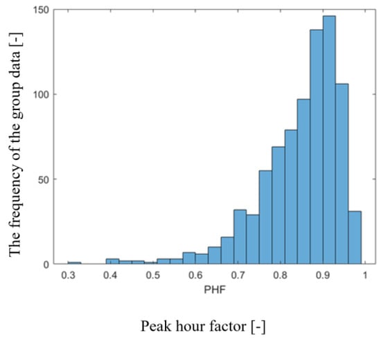
Figure 5.
Normal distribution peak hour factor (PHF—peak hour factor).
In the analysis of the occurrence of vehicle groups, the focus was on comparing the occurrence of vehicle groups in the traffic stream. The following figure, Figure 6, presents a comparison of the most numerous groups, with the total number of vehicles and the 85th percentile speed for each level of the traffic stream. The analysis shows that the average travel speed drops by almost 30% for the condition where groups of 25 or more vehicles are formed. In terms of the subjective perception of travel in the traffic stream at the edge of LOS C, a comparison of the identification of the multiplicity by the spacing of vehicles relative to each other was processed (Figure 6a). The data show that for groups with more than 20 members, the difference between groups with 2 s and 3 s group temporal identification decreases significantly (Figure 6b).
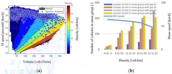
Figure 6.
Traffic flow data evaluation: (a) Evaluation of vehicle groups on urban streets; (b) Proportion at density limits by time gaps of 2 s, 3 s, 4 s, and 5 s and mean speed (85 till).
The presented evaluation was processed for all radars located on the road in question. When the intensity, and therefore the proportion of trucks, was kept constant, several differences were found. The individual disproportions in the traffic flow parameters describe the influence of the ambient conditions on the driving dynamics. In the subsequent part of the paper, multiparametric graphical representations of the number of groups (gap = 4 s) with the cumulative probability (Figure 7) of a given condition are expressed. The profiles are evaluated after traveling a distance of 5.5 km. The difference occurred mainly in the speed in the multiple groups, where the average speed differed by 5–10 km/h.
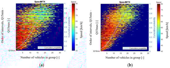
Figure 7.
Multiple parametric expressions of traffic flow characteristics: (a) Radar C1; (b) Radar C2.
Changes in the representation of vehicles in groups were verified by Friedmen’s test. The average values of the most represented group from two radars, separated by approx. 1 km on one section, in the given time intervals, was used as a basic set. Based on data analysis using a t-test, we determined that the difference in the efficiency of the occurrence of a dominant group of vehicles between radars C2 and C3 is statistically significant (p < 0.05), indicating that there is a probability of less than 5% that this difference is only random. This means that the representation of the dominant group on the road section changes and is not just a result of chance (p = 0.0027). This result is valid when identifying a group with a criterion of up to 2 and up to 5 s. A higher p-value than 0.05 was calculated for the peak hour period for the 3 s identification criterion (p = 0.0833). At 5 s, the dependence was still below 0.05.
Overtaking on the I/18 road near the village of Strečno was allowed in only one section, within the section marked by us as Castle Strečno at the junction of the lanes in the direction of Martin. At the time of the survey, there was a 2 + 1 lane combination at this location, which allowed overtaking.
Figure 8 and data in Table 2 indicate the amount and type of overtaking and overtaken vehicles in real values (y-axis). The graph contains a change of order (x-axis), where the value 0 represents vehicles that have maintained their initial position in the traffic flow, positive numbers to the right of it present overtaking vehicles, and negative numbers to the left of 0 represent overtaken vehicles. It can be seen in the graph that passenger vehicles, as well as a certain part of trucks, most often overtook and changed their position. The highest number of overtaking vehicles was recorded when the order was changed by three positions, namely, 47 passenger cars and 24 trucks.
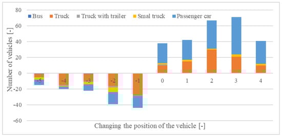
Figure 8.
Evaluation of vehicle overtaking.
Table 2.
Amount and type of overtaking and overtaken vehicles in real values.
Reducing the speed at exposed times will cause an increase in the density of the traffic flow. This may cause a difference between a compliant condition (with a density below 30 cars/km) and a non-compliant condition. A comparison of the two traffic conditions is shown in Figure 9.
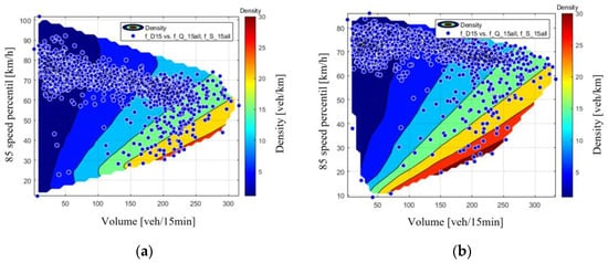
Figure 9.
Multiple parametric expressions of traffic flow density: (a) Radar C1; (b) Radar C2.
Another example is the evaluation of data from the climb to the mountain crossing on I/10. Evaluation of the data at the top of the climb confirms the influence of trucks, which influence the traffic flow. No significant differences emerge for the evaluation of vehicle group frequency identifiers. Vehicles travel at distances on the borderline of 5 s. In almost all groups, the truck is the group leader. The following figure, Figure 10, shows a comparison of group frequencies at the beginning and end of the climb. The course of the cumulative probabilities of congestion groups is different. At the beginning of the climb, maximum vehicle groups are formed with 20 vehicles. At the top of the climb, groups with 30 vehicles are observed, at the same traffic load.
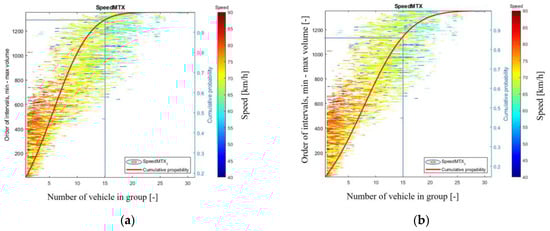
Figure 10.
Comparison of the probability of formation of platoons: (a) the start of the climb; (b) the top of the climb.
4. Discussion
Traffic flow in the area is affected by several factors. When the fundamental relationships between speed, intensity, and density of the traffic flow are valid, other surrounding influences can also be observed. The average travel speed may be influenced by direction, altitude, sight conditions, or weather. In practice, there is a requirement to demonstrate as close a match as possible between the modeled outputs and the real data. The main idea of this study was to develop an evaluation tool that can be used to identify the nature of the traffic flow at busy times. Results from traffic surveys were used as source data. These were carried out in the last five years with a record length of at least 7 days on the road infrastructure in the Slovak Republic.
In the first step, we identified profiles and time intervals in which intensity decreases and density increases occur. In particular, profile values were used to achieve the aforementioned objective. Out of the total number (60 radars), 12 sections did not comply with the threshold value, calculated in terms of TP 102. As traffic volume increases, groups of vehicles are formed. Identifying groups of vehicles in the traffic stream is difficult. The composition of the traffic (proportion of lorries), the inhomogeneous characteristics of the individual vehicles, and the different behaviors of the drivers are decisive. The design parameters of the road also influence the flow. Examples include the width of paved shoulders, curvature, etc. This type of data is not very difficult to parameterize in microsimulation models. The identification of groups according to the time intervals of consecutive vehicles in the recorded database was processed. Gaps smaller than 2 s, 3 s, 4 s, and 5 s were successively classified. Subsequently, the maximum number of vehicles per group was assigned. Using a computational algorithm in Matlab, it was possible to determine the frequency of each group at five- and fifteen-minute intervals using the four time gaps between vehicles. The above assessment is particularly relevant in assessing the flow of traffic at optimum volume. Depending on the surrounding area, it is possible to identify local specificities that will be reflected in the traffic flow. The identification of the formation of groups of vehicles under different spacing conditions is reflected in the space as a parameter evaluating the accepted spacing between vehicles. In the following research, we want to focus on sections that are on the edge of the capacity-compliant condition, but in the real environment, the traffic is subjectively evaluated as flowing.
In the next step, the dynamic nature of the occurrence of the groups was assessed according to the overall intensity. The results show a change in the traffic flow dynamics at unchanged intensity and the highest allowable design speed. The difference between the frequency of groups at 2 s and 5 s time values was significant, especially for suburban and regional roads. The graphical outputs presented declare the change in the proportion of vehicles traveling in a group. An example is the evaluation of a specific section where vehicles were redistributed into smaller groups after a change of width arrangement and during a short climb. In the presented example, a change of three vehicles in the mean value of the largest groups at the beginning and end of the section was measured. This means that for the same intensity, smaller groups were more frequent at the beginning of the section compared to the data at the end of the section. There were groups of vehicles recorded with a higher proportion of more numerous groups. This evaluation was performed for a time gap of 4 s.
The results further point to a different type of group formation at a comparable intensity during Wednesday and Friday (see Figure 11 and Table 3). This phenomenon was reflected in the evaluation of the normal distribution of the measured data. The highest average frequented group (12.8) was recorded on Wednesday. Almost identical average intensity was recorded on Wednesday and Friday. However, on Friday, a smaller average number of vehicles was recorded in the most frequented vehicle group. Almost the same average number of vehicles in the group was recorded on Sunday and Wednesday. However, the average intensity was higher on Sunday by approximately 50 vehicles per 15 min.
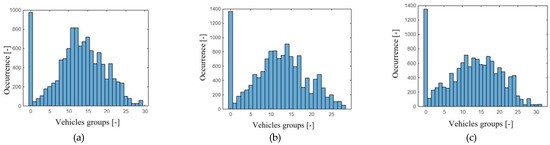
Figure 11.
Comparison of specific data of individual days (I/18): (a) Wednesday; (b) Friday; (c) Sunday.
Table 3.
Comparison of specific data of individual days (I/18).
Mountain-crossing sections were mainly affected by the proportion of trucks. Their influence on travel speed is addressed in the capacity assessment by a diagram depending on the length and magnitude of the climb or descent. The measured results show the possibility of detecting the modeled traffic and comparing it with reality by identifying groups of vehicles. By comparing the representation of the vehicle groups, it is possible to identify the impact of freight traffic on the mountain crossing, etc.
The presented methodology can also be applied to other tasks in traffic engineering. Time gap detections are essential data for the ramp metering setup of autonomous vehicles. Monitoring platoons at different levels of traffic density, together with variable traffic signing, can contribute to efficient traffic management. Several car-following models (Wiedemann model (1974) [27], Gipps’ model (Gipps, 1981) [28], DNN-based anticipatory driving model (DDS, 2021) [29], etc.) have been used in traffic simulation. Monitoring groups of objects in a traffic stream can be useful in related crowd-modeling studies. One study [30] describes the prediction of spatiotemporal flow using a new, integrated, and holistic knowledge map. Crowd flow prediction is thus of strategic importance for traffic management and public safety.
The output of the present paper is not the exact values of maximum intensities under specific conditions but a comprehensive analytical tool (in Matlab) that can be used to evaluate the impact of platoon formation in each location.
The potential applications of traffic flow analysis can be further applied in the continuous assessment of the share of individual vehicle groups in the traffic flow, in the assessment of road safety, or in the setup of microsimulation and emission models. An example of a comparison of the above-mentioned breakdown is shown in the following Figure 12. In the figures, the top row is the processed classification by group identification with a 2 s threshold. The bottom row is the identification with a 5 s threshold. The outputs during the measurement are shown on the left. The x-axis expresses the number of the 15 min interval; the y-axis expresses the frequency of occurrence of a given group. The presented analysis offers the possibility of defining time segments during the peak period. Such an evaluation is useful to demonstrate the impact of specific conditions on a traffic homogeneous segment with heterogeneous segmentation.
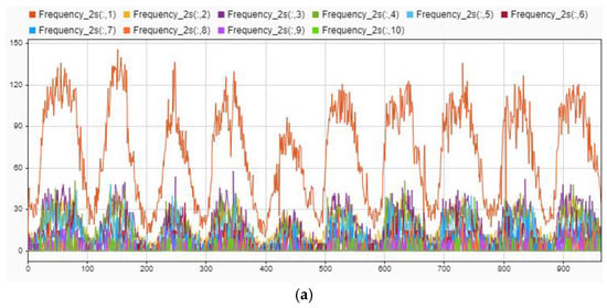
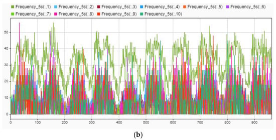
Figure 12.
Radar signal analyser of vehicle groups by Gapident (axis y) during observed time (axis x): (a) Gapident = 2 s; (b) Gapident = 5 s.
Continuous tracking can be further used for the development of vehicle–infrastructure cooperation technology. The real-time information interaction can be carried out between vehicles. According to Hallé et al. [31], research on vehicle group behaviors in the Connected Vehicles (CV) environment focuses on collaborative control and organization management optimization of vehicle platoons.
The formation of vehicle groups depends on several factors. The presented results are mainly based on congested sections. Groups of vehicles will be created based on intensity or, for example, acceleration noise. This study deals with different conditions on different profiles, which are parameterized according to the road manager’s database. The impact on the traffic stream is significant, especially from the point of view of possible communication between vehicles. The early formation of groups with different numbers of vehicles causes instability in the traffic flow. Using dynamic speed regulation, it is possible to increase the number of cars in a group but paradoxically stabilize the traffic flow.
As already mentioned, the next steps of the work with the traffic flow will be directed toward defining the boundary conditions for the change of the dominant group of vehicles at a certain intensity. As an example, the first microsimulation model can be given, where the measured section is divided into sections of 10 m. The analytical model in the Matlab program continuously displays the speed of vehicles (Figure 13). From the graphic display of the average speed of 10 m segments in a given time interval, it is possible to find the places where the speed decreases. In the next steps, the model will be supplemented with a control algorithm based on the recording of time intervals between vehicles on the profile. The aim is to increase the flow of traffic. The long-term goal of the research is the parameterization of environmental influences into traffic flow models. In microscopic modeling, it is possible to set safety distances of vehicles, acceleration, deceleration, etc. The probability of the formation of groups on individual sections of the model is reflected in the individual types of roads. This step is possible using a script for speed control on sensors in the network.
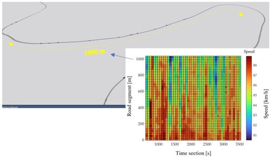
Figure 13.
Example of a graphical evaluation of the formation of platoons in a microsimulation over 3600 s.
5. Conclusions
A consequence of the ever-increasing degree of motorization is an increase in the share of individual car transport. Measures to increase the share of non-motorized or public transport are usually the main objective of transport studies of a territorial unit. The problem of congested sections is particularly acute for smaller towns on rural and regional routes. These sections generally follow longer routes, which are not always easy to modify in favor of increasing the attractiveness of public transport. There are sections of the road network that have problematic conditions despite a favorable capacity rating, or traffic is relatively smooth on the section despite an unfavorable capacity rating. The identification of traffic flow groups is one possible route.
Fundamental relationships of the main characteristics of the traffic flow determine and name the states of traffic flow. In the presented analysis, a direct evaluation tool for detecting groups of vehicles in the traffic stream has been developed. The direct output from the radar can indicate different traffic flow characteristics that result from local conditions, such as directional or elevation design of the route alignment.
This study confirmed the assumption of a dynamic process of creating vehicle groups. By detecting vehicles at the cross-section, it is possible to identify the stability of the traffic stream based on the formation of groups of vehicles. The described procedure makes it possible to detect and characterize the state of traffic based on the speed and number of dominant groups of vehicles. The highest differences were measured in places where the combination of no overtaking, short gradients, and layout affected the formation of groups of vehicles. In some cases, speed differences on neighboring radars of up to 30 km/h were measured, and these were at the same intensities. Values of traffic density on sub-sections change synergistically with speed. An increase in density of up to 26% was recorded on sections complicated by direction and slopes. In our analysis, we will continue to focus on precisely defining problem areas.
For regional roads, the cumulative probability of vehicle groups concerning the section’s occupancy was evaluated. The results show non-negligible changes in the probability of the emergence of dominant vehicle groups. The analysis shows that the average travel speed drops by almost 50% for the condition where groups of 25 or more vehicles are formed with a time interval of up to 4 s.
The fragmentation of the territory and different horizontal and height design parameters affect the ride. The type of roads and regions are included, especially for project parameters (narrower category, lower speed, or smaller directional and height curves). By creating a complex database, it is possible to determine the clues for calculating the probability of the formation of a column. However, the results must be verified by in situ measurement.
As a parallel effect, the impact on the emission load of the network will be assessed with respect to the speed adjustment. The presented evaluation according to the identification and analysis of time gaps will be further used in the analysis of the traffic flow with the help of artificial intelligence. For example, cutting-edge AI and computer vision techniques can accurately extract on-site vehicular trajectory-related data from videos [32].
Author Contributions
Conceptualization, M.D.; Methodology, M.C., J.C. and Z.P.; Data curation, M.D., M.C., J.C. and Z.P. All authors have read and agreed to the published version of the manuscript.
Funding
This research was funded by Slovak Research and Development Agency (APVV-21-0416, Grant Vega No. 1/0206/22).
Institutional Review Board Statement
Not applicable.
Informed Consent Statement
Not applicable.
Data Availability Statement
Data are contained within the article.
Acknowledgments
The paper is a result of the research supported by the research project APVV-21-0416, Research on mobility and emission attributes of the transport process (Výskum mobility a emisných atribútov dopravného procesu). This paper was also realized with support of project Grant Vega No. 1/0206/22, Research of traffic flow saturation effects to determine resistance functions (Výskum vplyvu saturačných efektov dopravného prúdu na funkcie zdržania).
Conflicts of Interest
The authors declare no conflict of interest.
References
- Hodoň, M.; Karpiš, O.; Ševčík, P.; Kociánová, A. Which Digital-Output MEMS Magnetometer Meets the Requirements of Modern Road Traffic Survey? Sensors 2021, 21, 266. [Google Scholar] [CrossRef]
- Eva, P.; Andrea, K. Determination of Priority Stream Volumes for Capacity Calculation of Minor Traffic Streams for Intersections with Bending Right-of-Way. Transp. Res. Procedia 2019, 40, 875–882. [Google Scholar] [CrossRef]
- Čulík, K.; Štefancová, V.; Hrudkay, K. Application of Wireless Magnetic Sensors in the Urban Environment and Their Accuracy Verification. Sensors 2023, 23, 5740. [Google Scholar] [CrossRef] [PubMed]
- Jakubec, M.; Lieskovská, E.; Bučko, B.; Zábovská, K. Comparison of CNN-Based Models for Pothole Detection in Real-World Adverse Conditions: Overview and Evaluation. Appl. Sci. 2023, 13, 5810. [Google Scholar] [CrossRef]
- Fang, X.; Péter, T.; Tettamanti, T. Variable Speed Limit Control for the Motorway–Urban Merging Bottlenecks Using Multi-Agent Reinforcement Learning. Sustainability 2023, 15, 11464. [Google Scholar] [CrossRef]
- Kováč, M.; Brna, M.; Decký, M. Pavement Friction Prediction Using 3D Texture Parameters. Coatings 2021, 11, 1180. [Google Scholar] [CrossRef]
- Slabej, M.; Grinč, M.; Kováč, M.; Decký, M.; Šedivý, Š. Non-Invasive Diagnostic Methods for Investigating the Quality of Žilina Airport’s Runway. Contrib. Geophys. Geod. 2015, 45, 237–254. [Google Scholar] [CrossRef]
- Jandacka, D.; Durcanska, D.; Cibula, R. Concentration and Inorganic Elemental Analysis of Particulate Matter in a Road Tunnel Environment (Žilina, Slovakia): Contribution of Non-Exhaust Sources. Front. Environ. Sci. 2022, 10, 952577. [Google Scholar] [CrossRef]
- Jandacka, D.; Decky, M.; Hodasova, K.; Pisca, P.; Briliak, D. Influence of the Urban Intersection Reconstruction on the Reduction of Road Traffic Noise Pollution. Appl. Sci. 2022, 12, 8878. [Google Scholar] [CrossRef]
- Gong, L.; Wang, T.; Lei, T.; Luo, Q.; Han, Z.; Mo, Y. Daily Travel Mode Choice Considering Carbon Credit Incentive (CCI)—An Application of the Integrated Choice and Latent Variable (ICLV) Model. Sustainability 2023, 15, 14809. [Google Scholar] [CrossRef]
- Crosbie, R.E.; Jakeman, T.; Lehmann, A.; Robinson, S.; Tolk, A.; Zeigler, B.P. Simulation Foundations, Methods and Applications; Springer: Cham, Switzerland; Available online: https://www.springer.com/series/10128 (accessed on 16 February 2024).
- Mahdi, M.B.; Alrawi, A.K.; Leong, L.V. Compatibility between Delay Functions and Highway Capacity Manual on Iraqi Highways. Open Eng. 2022, 12, 359–372. [Google Scholar] [CrossRef]
- Suvin, P.V.; Mallikarjuna, C. Modified Generalized Definitions for the Traffic Flow Characteristics under Heterogeneous, No-Lane Disciplined Traffic Streams. Transp. Res. Procedia 2018, 34, 75–82. [Google Scholar] [CrossRef]
- Darwish, T.; Abu Bakar, K. Traffic Density Estimation in Vehicular Ad Hoc Networks: A Review. Ad Hoc Netw. 2015, 24, 337–351. [Google Scholar] [CrossRef]
- Elefteriadou, L. An Introduction to Traffic Flow Theory; Springer: New York, NY, USA, 2014; Volume 84, ISBN 978-1-4614-8434-9. [Google Scholar]
- Maerivoet, S.; De Moor, B. Traffic Flow Theory. arXiv 2005, arXiv:physics/0507126v1. [Google Scholar]
- Verkeerscentrum Vlaanderen, Departement Leefmilieu En Infrastructuur, Administratie Wegen En Verkeer, Vuurkruisenplein 20, 2020 Antwerpen. MINDAT—Databank Ruwe Verkeersdata Vlaams Snelwegennet—2001 En 2003. Available online: https://www.verkeerscentrum.be/ (accessed on 11 December 2023).
- Romana, M.G.; Hernando, D. Obtaining a Maximum AADT Sustained by Two-Lane Roads: An Application to the Madrid Region in Spain. Transp. Res. Procedia 2016, 14, 3209–3217. [Google Scholar] [CrossRef][Green Version]
- Zegeer, C.V.; Deacon, J.A. Effect of Lane Width, Shoulder Width, And Shoulder Type on Highway Safety. State Art Rep. 1990, 6, 1–21. [Google Scholar]
- Čelko, J.; Decký, M.; Kovac, M. An Analysis of Vehicle-Road Surface Interaction for Classification of IRI in the Frame of Slovak Pms. Eksploat. I Niezawodn. 2009, 41, 15–21. [Google Scholar]
- ZSK Strategy for Creating and Building an Integrated Transport System in the Zilina Region (Stratégia Tvorby a Budovania Integrovaného Dopravného Systému v ŽSK). Available online: http://enviroportal.sk/eia/dokument/252189 (accessed on 11 July 2022).
- Qian (Sean), Z.; Li, J.; Li, X.; Zhang, M.; Wang, H. Modeling Heterogeneous Traffic Flow: A Pragmatic Approach. Transp. Res. Part B Methodol. 2017, 99, 183–204. [Google Scholar] [CrossRef]
- Novačko, L.; Babojelić, K.; God, N.; Babić, L. Estimation of Modal Split Parameters—A Case Study. Trans. Motauto World 2020, 5, 51–53. [Google Scholar]
- Babic, L.; Tišljaric, L.; Vrbanic, F.; Novacko, L. Autonomous Vehicles Parameter Influence on Mixed Traffic Flow on a Motorway: A Simulation Approach. Transp. Res. Procedia 2022, 64, 149–156. [Google Scholar] [CrossRef]
- Harrou, F.; Zeroual, A.; Hittawe, M.M.; Sun, Y. Traffic Congestion Detection: Data-Based Techniques. Road Traffic Model. Manag. 2022, 141–195. [Google Scholar] [CrossRef]
- Kocianova, A. Calculation of the Capacities of Roads; The Ministry of Transport of the Slovak Republic: Bratislava, Slovakia, 2015; Available online: https://www.ssc.sk/files/documents/technicke-predpisy/tp/tp_102.pdf (accessed on 16 February 2024).
- Higgs, B.; Abbas, M. Alejandra Medina Analysis of the Wiedemann Car Following Model Over Different Speeds Using Naturalistic Data. 2011. Available online: https://onlinepubs.trb.org/onlinepubs/conferences/2011/RSS/3/Higgs,B.pdf (accessed on 11 December 2023).
- Gipps, P.G. A Behavioural Car-Following Model for Computer Simulation. Transp. Res. Part B Methodol. 1981, 15, 105–111. [Google Scholar] [CrossRef]
- Isha MK, F.; Shawon MN, H.; Shamim, M.; Shakib, M.N.; Hashem MM, A.; Kamal MA, S. A DNN Based Driving Scheme for Anticipatory Car Following Using Road-Speed Profile. In Proceedings of the 2021 IEEE Intelligent Vehicles Symposium (IV), Nagoya, Japan, 11–17 July 2021; pp. 496–501. [Google Scholar]
- Xiao, G.; Chen, L.; Chen, X.; Jiang, C.; Ni, A.; Zhang, C.; Zong, F. A Hybrid Visualization Model for Knowledge Mapping: Scientometrics, SAOM, and SAO. IEEE Trans. Intell. Transp. Syst. 2023, 1–14. [Google Scholar] [CrossRef]
- Hallé, S.; Chaib-draa, B. Collaborative Driving System Using Teamwork for Platoon Formations. In Applications of Agent Technology in Traffic and Transportation; Birkhäuser-Verlag: Basel, Switzerland, 2005; pp. 133–151. [Google Scholar]
- Chen, X.; Wang, Z.; Hua, Q.; Shang, W.-L.; Luo, Q.; Yu, K. AI-Empowered Speed Extraction via Port-Like Videos for Vehicular Trajectory Analysis. IEEE Trans. Intell. Transp. Syst. 2023, 24, 4541–4552. [Google Scholar] [CrossRef]
Disclaimer/Publisher’s Note: The statements, opinions and data contained in all publications are solely those of the individual author(s) and contributor(s) and not of MDPI and/or the editor(s). MDPI and/or the editor(s) disclaim responsibility for any injury to people or property resulting from any ideas, methods, instructions or products referred to in the content. |
© 2024 by the authors. Licensee MDPI, Basel, Switzerland. This article is an open access article distributed under the terms and conditions of the Creative Commons Attribution (CC BY) license (https://creativecommons.org/licenses/by/4.0/).