Multiscale Analysis for Identifying the Impact of Human and Natural Factors on Water-Related Ecosystem Services

Abstract

Accurately identifying and obtaining changes in ecosystem drivers and the spatial heterogeneity of their impacts on ecosystem services can provide comprehensive support information for ecological governance. In this study, we investigate the changes in the relationship between human and natural factors and water-related ecosystem services (WESs) in different sub-watersheds across various time periods, focusing on four aspects: single-factor effect, nonlinear effect, interactive effects, and spatial characteristics. Taking the southern basins, which have complex topographic, climatic, and economic characteristics, as a study area, the study area was divided into four sub-basins with different characteristics. WESs of water yield, soil conservation, and water purification were quantified using the InVEST model for five periods from 2000 to 2020, and the OPGD and MGWR models were integrated to assess the impacts of 15 factors on WESs and their spatial characteristics. The results show the following: (1) After comparing the data over multiple time periods, climate factors such as precipitation (0.4033) are the primary factors affecting WESs in the southern basins, and human factors such as construction area (0.0688) have a weaker influence. The direct impact of human factors on WESs is not significant in the short term but increases over time. (2) Different sub-watersheds have different impacts on WESs. For instance, human activity intensity (0.3518) is a key factor affecting WESs in the Inward Flowing Area, while precipitation is the primary factor influencing WESs in other sub-watersheds. (3) Influencing factors and WES changes are often nonlinearly correlated; however, once a certain threshold is exceeded, they may have adverse impacts on WESs. (4) When a single factor interacts with other factors, its explanatory power tends to increase. (5) Compared to traditional methods, the estimation accuracy of MGWR is higher. Intense human activities can adversely affect WESs, while abundant precipitation creates favorable conditions for the formation of WESs. Therefore, integrating long-time-series multi-remote sensing data with OPGD and MGWR models is suitable for identifying and analyzing the driving mechanisms of human and natural factors that influence changes in WESs. Against the backdrop of global change, elucidating the driving factors of ecosystem services can provide crucial insights for developing practical policies and land management applications.

1. Introduction

The concept of ecosystem services (ESs) was initially introduced by Costanza et al. [1] and has developed into a significant ecological concept [2]. ESs refer to the benefits that organisms derive from ecological activities, playing essential roles in sustaining Earth’s life-support systems [3]. ESs are a vital link between natural ecosystems and human society, contributing positively to the well-being and livelihoods of humans [1]. Nevertheless, in response to the requirements of social development, policies have been enacted to alter land use and land cover (LULC) patterns, exerting an impact on ecosystems and resulting in an imbalance among them [4]. The findings of the Millennium Ecosystem Assessment (MA) [5] indicate an alarming approximately 60% decline in ESs over the past half-century. This trend indicates that the sustainability of ecosystems has been severely compromised, which will profoundly affect human well-being and the sustainable development of complex socio-economic–ecological systems. Therefore, understanding the trends of long-time ecosystem dynamics and studying their driving factors and spatial heterogeneity have become research hotspots, crucial for decision-makers to manage ecosystems reasonably and optimize the comprehensive benefits of natural ecosystems and human social–economic systems.

The fragility of ESs makes them inherently unstable and vulnerable to the combined impacts of natural change and human activities [6,7]. Natural change exerts an impact on the provisioning of ESs by altering their structure and functioning. For example, climate regulation, nutrient cycling, soil formation, and photosynthesis provided by ESs are threatened by extreme climate events [8,9]. Ali et al. [10] forecasted that global warming will heighten the risk of extreme precipitation and flooding in basins. LULC changes induced by human activities are another significant driver that impacts the distribution of ESs and their capacity to provide these services [11]. Studies have demonstrated that LULC transformations, especially in growing urban regions, noticeably affect ecosystem services due to modifications in carbon equilibrium and nutrient circulation [12]. Continuing urban development has led to population agglomeration and economic acceleration, intensifying stress on ESs and generating various issues that jeopardize the proper functioning of natural ecosystems [1]. Conversely, challenges such as the deterioration of water-related ecosystem services (WESs), scarcity of resources, and escalating ecological vulnerability have diminished the quality of urbanization, impeding the healthy and sustainable development of cities [13]. At the same time, climate- and human-induced damage to ecosystem services has worsened, which is projected to pose a growing threat to ecosystem services and biodiversity and is expected to become even more severe over the next decade [14]. Hence, a comprehensive understanding of the factors influencing WESs can provide scientific guidance for the management of ecosystem services and the optimization of decision-making processes [15].

To address these limitations, statistical methods such as regression analysis [16], correlation analysis [17], factor analysis [18], cluster analysis [19], and multivariate analysis [20] have been developed to analyze the impact of various factors, including human and climate factors, on ecosystems and their services. These approaches help identify key drivers, quantify the relationships between variables, and provide insights into the complex interactions between humans, the climate, and ecosystem services [21]. Despite their utility, these methods have certain limitations. They tend to consider single-factor importance and simple factors, making it difficult to capture the complex interactions among variables. Additionally, these methods may not be able to quantify the contribution of individual influencing factors or account for multivariate covariance, which can lead to an incomplete or biased understanding of the underlying phenomena [22]. The geographical detector model (GDM) offers a robust approach to addressing these challenges by effectively identifying the contribution of single factors and the interactions between drivers. The GDM is designed to mitigate the limitations of traditional statistical methods, enabling a more comprehensive understanding of the complex relationships between humans, the climate, and ecosystem services [23]. For example, Fang et al. [24] advanced GDM to identify natural and anthropogenic impacts on ecosystem services; Wang et al. [25] used GDM to analyze ecosystem service drivers; Zhang et al. [26] advanced GDM to analyze the impact mechanism of water ecological service value. While the GDM represents a significant advance in exploring the driving forces of ecosystem change, it does have certain inherent limitations. One of the limitations is that GDM does not directly reflect the spatial heterogeneity of impact factors on ecosystem change [27]. In addition, traditional GDM primarily utilizes empirical knowledge for classifying spatial data, which can often be subjective. To address these limitations, the demonstration of spatial variation can be addressed by geographically weighted regression (GWR) [28]. GWR investigates the spatial heterogeneity of processes and relationships by employing a series of localized regression models. Multiscale geographically weighted regression (MGWR) enhances the standard GWR by accounting for spatial variations in the effects of factors. This improvement enhances the robustness and accuracy of the model [29]. Furthermore, we introduce the optimal parameter geographic detector (OPGD), which selects the combination of classification parameters with the highest q value to discretize continuous variables, enhancing the quantitative research on the balanced driving mechanism of ESs [30]. Meanwhile, previous studies analyzing the impacts on ESs primarily focused on the changes between the initial and final periods, without considering the changes in ESs during the intervening periods. Therefore, combining OPGD with MGWR based on long time data can more accurately characterize the direction and intensity of different factors influencing WESs. Currently, there are no available studies that incorporate both the OPGD and MGWR models to investigate the driving influence and spatial characterization of impact factors on WESs.

Previous research has indicated that, among various categories of ESs, WESs are most closely related to human welfare [31]. WESs are generated by interactions between terrestrial ecosystems and hydrological processes and are essential for complying with human needs and maintaining ecosystem health [32]. WESs can be classified into various types of ESs. In particular, WESs deliver water resources for human usage (supply services), have an important influence on soil and biodiversity conservation (supporting services), contribute to water cycling and cleaning (regulation services), and provide natural landscapes for ecotourism along rivers and lakes (cultural services) [33]. The establishment of cities and the persistence of human societies are intricately connected to water, a vital element that dictates the survival and development of species. Additionally, water plays a pivotal role in shaping the activities of urban populations, industries, and other economic sectors [34,35]. Rapid urbanization directly or indirectly affects the aquatic environment and reduces the capacity of WESs to provide important ESs [36,37]. This may lead to environmental damage, depletion of water resources, and fragmentation and degradation of WESs. The integrated valuation of ecosystem services and trade-offs (InVEST) model is a well-established method for evaluating the three WESs mentioned above and has been applied in many empirical studies in different regions [38,39,40]. Simultaneously, comparisons among different regions can offer constructive suggestions for regional management, mitigate negative impacts, and promote sustainable regional development. However, knowledge gaps still exist in comparative studies of WES drivers, and comparisons among various regions are lacking. Therefore, it is necessary to quantify the temporal dynamics between human and natural factors and the driving factors of WESs at different scales to develop reasonable regional policies.

The WESs in China’s southern basins are complex, with significant disparities in terms of natural and human influence across different river basins. Meanwhile, the Yangtze River Basin (YRB) and Pearl River Basin (PRB) are important water sources and lifelines for the country, so the Chinese Government attaches great importance to protecting the ecological balance of the southern basins. However, as socio-economic development continues and human activities and natural change take their toll on WESs, various policies, such as the conversion of farmland to forests and ecological restoration, have been implemented to address these issues. Nevertheless, identifying the critical factors affecting WESs and their spatial characteristics and formulating informed recommendations based on these findings present a significant challenge for decision-makers.

To address the knowledge gaps in previous studies on the quantitative impact values and spatial heterogeneity of WESs from multiple remotely sensed images under long time series, this study focuses on two key areas: (1) evaluating the spatial distribution, changing trends, and hotspot characteristics of the ecological environment and WESs over a long time scale and (2) integrating the OPGD and MGWR models based on long-time-series multi-remote sensing data to explain the impact of human and climate factors on the spatial variation of WESs of different socio-economic and natural basins at different temporal and spatial scales. In the context of global environmental change and the development of the eco-economy, a systematic analysis of the dynamics of driving factors can provide theoretical scientific support for ecosystem decision-making in regions with different natural characteristics and economic development stages.

2. Materials and Methods

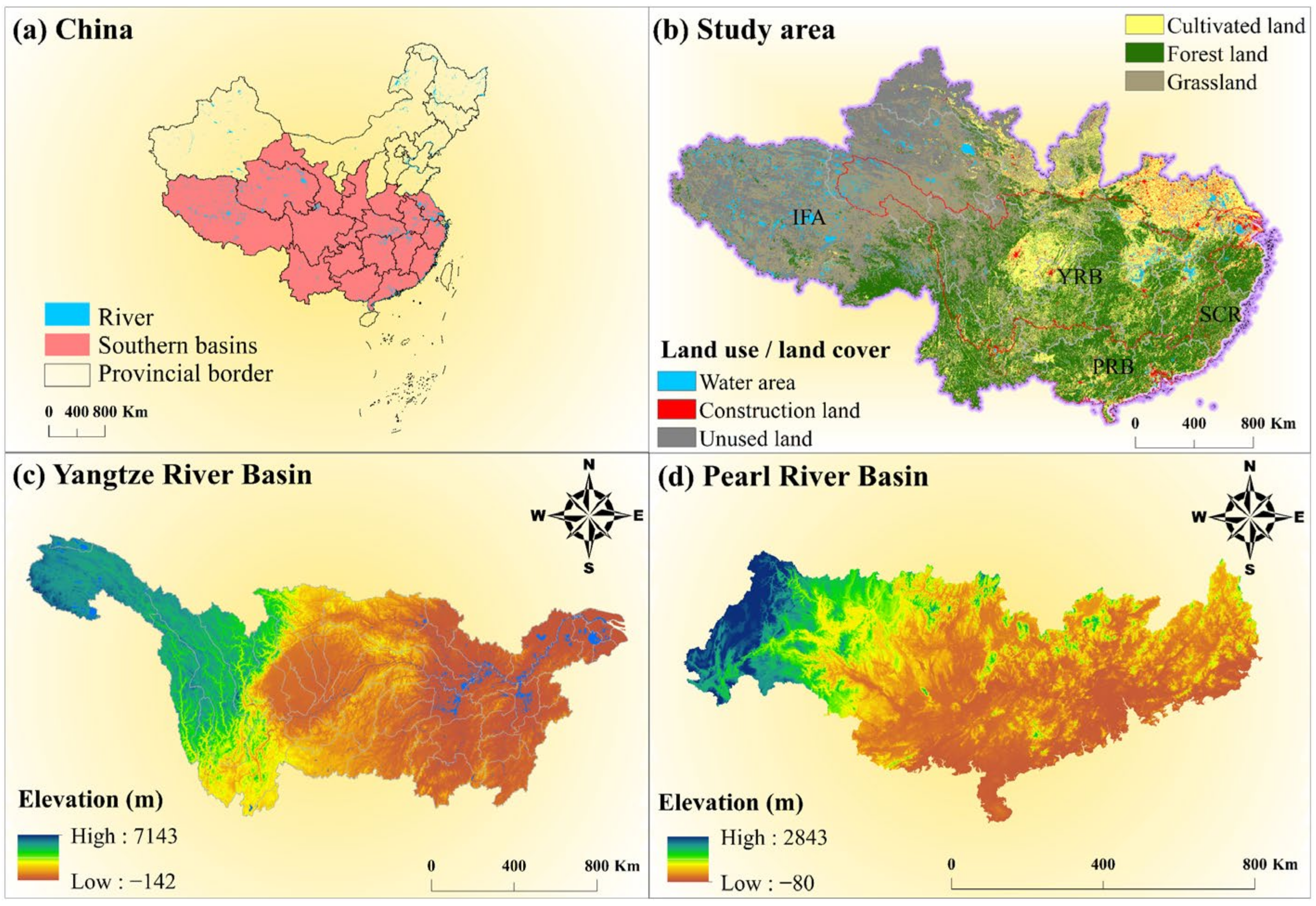
2.1. Study Region

The southern basins of China are the target basins for the analysis (Figure 1) and include the YRB, PRB, Inward Flowing Area (IFA), and Southeast Coastal River Basin (SCR). These basins, originating from the Qinghai–Tibet Plateau, share similarities in terms of geographical location, climatic characteristics, and abundant water resources, all of which play crucial roles in supporting agriculture, industry, and residential life. However, they also exhibit notable differences in terms of climate type, economic development, and ecological environment levels. In terms of climate conditions, YRB, PRB, and SCR have humid climates with ample rainfall, whereas IFA has a comparatively drier climate with less rainfall. Economically, YRB, PRB, and SCR are among the most developed regions in China, while IFA lags behind in economic development. In terms of natural resources, YRB and PRB are rich in water resources, forest resources, and mineral resources, while SCR and IFA have relatively fewer natural resources. Ecologically, YRB, PRB, and SCR have relatively sound ecological environments, boasting numerous wetlands and nature reserves, whereas the ecological environment of IFA is comparatively fragile. Due to the combined impact of ongoing social and economic development, urbanization, climate change, and human activities, some areas within the southern basins of China have experienced significant environmental and water resource issues. Due to limitations in spatial availability and natural resources, urban centers do not form continuous aggregations. The distinct ecological environments and economic conditions of the four river basins determine that their future demand development patterns will inevitably differ. Promoting high-quality development in different river basins and constructing a modern economic system are the top priorities in basin construction. Seizing the opportunities presented by ecological protection and high-quality development, exploring a path towards coordinated basin development should be pursued.

2.2. Data Sources and Preprocessing

Table 1. Description of the datasets used in this study.

Dataset	Source	Spatiotemporal Resolution	Source/Download Site
Land use and land cover (LULC)	Institute of Geographic Sciences and Natural Resources Research, China	30 m	http://www.resdc.cn/, accessed on 19 September 2023
DEM	Geospatial Data Cloud Platform	30 m	http://www.gscloud.cn/, accessed on 21 September 2023
Soil	Resource and Environment Science and Data Centre	1000 m	http://www.resdc.cn/, accessed on 22 September 2023
Temperature (TEM), relative humidity (REH), precipitation (PRE), evaporation (EVA), sunshine duration (SUN)	China Daily Surface Climate dataset (V3.0)	/	China Meteorological Data Website (http://data.cma.cn, accessed on 11 September 2023)
Normalized Difference Vegetation Index (NDVI)	Resource and Environment Science and Data Center	1000 m	http://www.resdc.cn/, accessed on 19 September 2023
Vegetation-available water content	$\begin{array}{l}PAWC=54.509-0.132sand\%-0.003{(sand)}^2-0.055silt\%\\ -0.006{(silt)}^2-0.738clay\%+0.007{(clay\%)}^2\\ -2.688OM\%+0.501{(OM\%)}^2\end{array}$
	where, PAWC represents the water content available to plants, while sand, silt, and clay denote the proportions of gravel, silt, and clay in the soil, respectively. OM represents the soil’s organic matter content.
Annual rainfall erosivity	$R_n=0.0534P_n^{1.6548}$
	where, Rn is the rainfall erosivity of the n-th year; Pn is the rainfall in the n-th year.
Soil erodibility	$\begin{array}{l}K=\left\{0.2+0.3\exp \left[-0.0256SAN(1-SIL/100)\right]\right\}\times {\left[SIL/(CLA+SIL)\right]}^{0.3}\\ \times \left\{1-0.25C/(C+e^{3.72-2.95C})\right\}\times \left(1-0.7SN1/(S{N}_1+e^{-5.51+22.9S{N}_1})\right)\end{array}$
	where, K represents soil erodibility, wherein a higher K value denotes lower corrosion resistance, and conversely, a lower value indicates higher resistance. The outcome is then multiplied by 0.1317 to standardize it in the international system of units. SAN, SIL, and CLA represent the sand, silt, and clay content, respectively, in the soil particle classification standard. SN1 is calculated as 1 minus SAN divided by 100. Additionally, C signifies the organic carbon content.

reports the specifications of the data employed for the quantification of the WESs and to derive the influence of human and natural factors on WESs. LULC (Figure 2), climatic, topographic (Figure 3), soil, and socio-economic datasets (Figure 4 and Figure 5) from 2000 to 2020 were used in the study.

Ecological data included LULC, climatic, NDVI, and hydrological data. The LULC data for 2000, 2005, 2010, 2015, and 2020 were sourced from the Chinese Institute of Geographic Sciences and Natural Resources Research (http://www.resdc.cn/, accessed on 19 September 2023) at a 30 m spatial resolution and classification accuracy exceeding 94.3%. Wetlands included paddy fields in cropland, natural water, reservoirs and ponds, total flats of water bodies, and marshes. Annual climatic data obtained from the National Meteorological Information Centre (http://data.cma.cn/, accessed on 11 September 2023) included temperature (TEM), precipitation (PRE), evaporation (EVA), relative humidity (REH), and sunshine duration (SUD). ANUSPLINE version 4.4 [41] was employed to read, merge, check, and count the data; generate spatial interpolation batch codes; and interpolate 1 km spatial raster data to grid data. Moreover, 30 m digital elevation models (DEMs) were sourced from the Geospatial Data Cloud Platform (http://www.gscloud.cn/, accessed on 21 September 2023). ArcSWAT version 2012.10.26 was then used for the elevation extraction and delineation of the basin. Soil data (e.g., clay, sand, silt, organic carbon, and soil PH percentage) were obtained from the Resource and Environment Science and Data Centre (http://www.resdc.cn/, accessed on 22 September 2023), and nighttime-light data (NLD) were obtained from the Prolonged Artificial Nighttime-light Dataset of China (PANDA) [42], both of which belong to the National Tibetan Plateau Data Center (http://www.tpdc.ac.cn/zh-hans/, accessed on 23 September 2023). The vegetation dataset comprised the monthly 1 km Normalized Difference Vegetation Index (NDVI) spatial distribution dataset in China from the Resource and Environment Science and Data Center (http://www.resdc.cn/, accessed on 19 September 2023). Runoff data from hydrological stations and hydrological statistics for the corresponding years were sourced from the China Water Resources Bulletin.

The socio-economic datasets comprised the average annual population density (POP), gross domestic product (GDP), and built-up areas, with spatial resolutions based on the core-set resolution of the datasets. The POP and GDP datasets were obtained from LandScan Global Population Data (https://landscan.ornl.gov/landsan-datasets, accessed on 23 September 2023) and the Resource and Environment Science and Data Center (http://www.resdc.cn/, accessed on 23 September 2023). The processing was performed in Python 2.7, R version 4.3.2 (R Core Team), and ArcGIS 10.6 (ESRI).

2.3. Quantification of Water-Related Ecosystem Services

2.3.1. Water-Related Ecosystem Service Selection

Basins play a vital role in providing essential ecosystem services to human societies, mainly by supplying pure freshwater from upstream sources [43]. However, LULC and climate change can greatly affect the ability of basins to regulate the hydrological cycle and control water quantity and quality. For example, deforestation, urbanization, and agricultural expansion can lead to increased water consumption, reduced infiltration, and lower water quality, while changes in climate patterns can lead to more frequent and intense droughts or floods. These changes can have significant impacts on the ecosystem services provided by basins, including the supply of clean water [44]. Water purification is an essential ecosystem service that basins provide. It involves the natural processes that remove contaminants and improve the quality of water, making it safe for human consumption and other uses. Water purification services are critical for maintaining the health of aquatic ecosystems and supporting human well-being [45]. Meanwhile, water yield (WY), soil conservation (SC), and water purification (WP) were among the most researched WESs by scholars [46,47,48]. Therefore, three specific water resource factors have been selected for this paper, namely WP, SC, and WP.

We utilized climate, soil, and rainfall erosion indices from the InVEST 3.9.0 software [49] to assess these factors.

Table 2. Biophysical coefficients in the InVEST models.

Description	Subclasses	root_depth	Kc	LULC_veg	Usle_c	usle_p	load_n	eff_n	crit_len_n	Load_p	eff_p	Crit_len_p
cultivated land	paddy field	300	1.1	1	0.3	0.2	15.5	0.25	30	1.73	0.25	30
	dry land	1000	0.7	1	0.35	0.3	15.5	0.25	30	1.73	0.25	30
forest land	forest land	3500	1	1	0.006	1	2.5	0.7	300	0.15	0.7	300
	shrubbery	1500	0.8	1	0.01	1	2.5	0.7	300	0.15	0.7	300
	sparse forest land	3500	0.9	1	0.017	1	2.5	0.7	300	0.15	0.7	300
	other forest land	3500	1	1	0.06	1	15.5	0.7	300	1.73	0.7	300
grassland	high coverage grassland	800	0.7	1	0.02	1	6	0.48	150	0.8	0.48	150
	medium coverage grassland	800	0.65	1	0.04	1	6	0.48	150	0.8	0.48	150
	low coverage grassland	800	0.6	1	0.1	1	6	0.48	150	0.8	0.48	150
water area	river and canal	1	1.05	0	0	0	0.001	0.05	30	0.001	0.05	30
	lake	1	1.05	0	0	0	0.001	0.05	30	0.001	0.05	30
	reservoir pond	1	1.05	0	0	0	0.001	0.05	30	0.001	0.05	30
	permanent glacier snow	1	0.5	0	0	0	0.001	0.05	30	0.001	0.05	30
	beach	1	1.05	0	0	0	0.001	0.05	30	0.001	0.05	30
	swampland	500	1.1	0	0	1	0.001	0.05	30	0.001	0.05	30
construction land	urban land	1	0.43	0	0	0	11	0.05	30	1.8	0.05	30
	rural residential area	1	0.5	0	0	0	11	0.05	30	1.8	0.05	30
	other construction	1	0.35	0	0	0	11	0.05	30	1.8	0.05	30
	bare land	1	0.5	0	1	1	11	0.05	30	0.36	0.05	30
unused land	stone land	1	0.5	0	0	1	11	0.05	30	1.8	0.05	30

Root_depth (mm): maximum root depth applicable to vegetated LULC types, measured in millimeters. Kc: plant evapotranspiration coefficient specific to each LULC type. LULC_veg: code indicating the vegetative status of the LULC class, specifically for Actual Evapotranspiration (AET) purposes. Usle_c: cover-management factor used in the Universal Soil Loss Equation (USLE), with values ranging between 0 and 1. Usle_p: support practice factor in the USLE, also ranging between 0 and 1. Load_[NUTRIENT]: nutrient loading measured in kg/ha/year corresponding to each LULC type. Eff_[NUTRIENT]: maximum nutrient retention efficiency, allowing the largest proportion of nutrients to be retained within the respective LULC category. Crit_len_[NUTRIENT]: the distance beyond which a patch of a specific LULC type is assumed to retain nutrients at maximum capacity, measured in meters. Suffixes “_n and _p” denote nitrogen and phosphorus, respectively.

lists the biophysical coefficient parameters.

2.3.2. Water Yield

The annual WY module within the InVEST model relies on a water balance estimation method utilizing PRE, reference EVA, LULC, plant-available water content, and root-restricting layer depth. The model’s calculated WY (Equation (1)) underwent validation through a comparison with actual runoff.

$$Y_i=\left(1-\frac{AE{T}_i}{P_i}\right)\times P_i$$

(1)

where, Y_i represents the annual WY (mm) of each grid cell i, AET_i is the actual annual EVP (mm), and P_i denotes the annual PRE (mm).

The RSME (Root Mean Square Error) between the modeled values (as shown in

Table 3. Comparison between observed data and modeled data of annual water yield.

River		2000	2005	2010	2015	2020
Xiangjiang River	Observed data	764.53	713.03	822.85	824.05	641.02
	Modeled data	813.08	759.14	945.41	816.62	625.07
	Error rate/%	−6.35	−6.47	−14.89	0.9	2.49
Yuanjiang River	Observed data	630.63	535.76	683.23	734.79	937.72
	Modeled data	739.02	540.65	748.99	781.9	929.36
	Error rate/%	17.19	−0.91	−9.63	−6.41	0.89
Zishui River	Observed data	243.33	247.59	241.78	227.45	283.55
	Modeled data	222.86	269.56	244.15	238.59	278.03
	Error rate/%	8.41	−8.87	−0.98	−4.90	1.95
Lishui River	Observed data	131.03	109.60	163.32	154.63	227.36
	Modeled data	143.34	119.39	175.41	167.50	205.85
	Error rate/%	−9.40	−8.93	−7.40	−8.32	9.46
Dongting Lake Basin	Observed data	2184.81	2105.03	2450.17	2501.27	2803.21
	Modeled data	2016.27	2009.27	2505.49	2092.97	2667.79
	Error rate/%	7.71	4.55	−2.26	16.32	4.83

Note: The observed data were sourced from the Changjiang & Southwest Rivers Water Resources Bulletin, available at http://www.cjw.gov.cn/zwzc/bmgb/, accessed on 22 November 2023.

) and the observed values is minimized at 50.13 when the parameter Z is set to 0.86.

2.3.3. Soil Conservation

The sediment delivery ratio module calculates the annual soil loss for each image element by employing the Universal Soil Loss Equation (USLE). It is expressed as the following equation:

$$RKL{S}_x=R_x\cdot K_x\cdot L{S}_x$$

(2)

$$USL{E}_x=R_x\cdot K_x\cdot L{S}_x\cdot C_x\cdot P_x$$

(3)

$$SEDRE{T}_x=RKL{S}_x-USL{E}_x$$

(4)

where, SEDRET_x represents the actual soil conservation at pixel x, RKLS_x represents potential soil erosion, USRL_x is the average annual soil erosion, R_x is the rainfall coefficient, K_x is the soil erosion coefficient, LS_x is the field topography coefficient, C_x is the planting and management coefficient, and P_x is the coefficient of the supporting conservation measures. The accuracy of the calculation results was verified by comparing them with the measured annual soil erosion in the experimental runoff area (

Table 4. Comparison between measured and calculated values of the amount of annual soil erosion in 2015.

Measured Value		Calculated Value		Error Rate/%
LULC	Soil Loss/Tons·km−2·yr−1	LULC	Soil Loss/Tons·km−2·yr−1
Economic fruit tree	1223.32	Forestland	1441.49	17.83
Greening grassland	1162.59			23.99
Bare land	1972.89			−26.94
Average	1452.93			−00.79

Note: The measured data were taken from the Lianhe runoff monitoring station (located at 111°22′00″ E, 27°03′00″ N).

).

2.3.4. Water Purification

WP is an essential service provided by ecosystems, and in measuring WP, the relative export of total dissolved nitrogen is focused on as a proxy for pollution. WP refers to the ability of ecosystems to mitigate water pollution by retaining some non-point-source pollutants through the action of vegetation and soils. LULC has a major impact on water quality by affecting the nutrients in surface water. The NE or PE per pixel on the landscape x can be calculated using Equations (5)–(7).

$$N\_expor{t}_i=loa{d}_i\times ND{R}_i$$

(5)

where, N_export_i is the nutrient (N or P) export on pixel i, load_i is the modified nutrient load on pixel i, and NDR_i is the nutrient delivery ratio on pixel i.

Due to the lack of measured data on NE and PE, the accuracy of the results of the study was mainly achieved by referring to published model parameters for a particular area within the study area [50].

2.3.5. Water-Related Ecosystem Services

To measure WESs, the above four WESs are integrated into a comprehensive index. According to the different dimensions of WESs, we standardized the individual WESs (WY, SC, NE, and PE) with a uniform value between 0 and 1 and then weighted and summed the four types of WESs. The formula is as follows:

$$WES{s}_j={\displaystyle \sum _{i=1}^m{w}_i{E}_{ij}}$$

(6)

where, WESs_j is the composite value of WESs in the j-th year and w_i represents the weight of type i of WESs. E_ij represents the normalized value of the i-th type of WESs in the j-th year. This study provides equal weight for the four categories of WESs because they are of equal importance.

2.4. Correlation Analysis of WES across Different Basins

We explored the spatial trends of the WES supply and its corresponding changing characteristics in the study area from 2000 to 2020, taking into account both natural and socio-economic systems. Based on the spatiotemporal characteristics of WES, the dynamic correlation of WES changes in each region was then investigated. The research concept and general design are summarized in the following (Figure 6). The framework consists of three key components:

(i)

WES calculation. With reference to the MA framework and the Common International Classification of Ecosystem Services (CICES), and considering the ecological properties of the study area, WY, SC, and WP were selected as the WES in this study. The correlation of the four factors was analyzed by using Spearman’s correlation, and the honorary data were excluded. The spatial map of WES supply from 2000 to 2020 was determined using the corresponding ecological model (Section 2.3.4). Global autocorrelation and local autocorrelation were used to analyze the spatial distribution of hot and cold spots of WES from 2000 to 2020.

(ii)

Impact strategies for long-term serial transformation analysis. Natural, anthropogenic, and WES data were evaluated from 2000 to 2020 using Sen’s slope estimator and the Mann–Kendall test.

(iii)

The interactions of composite factors affecting WES changes were explored using OPGD and MGWR models to understand the key drivers, synergistic impact effects, spatial variability, and magnitude of WES impacts in terms of spatial heterogeneity contributions, as well as driving and constraining relationships under long-time-series trends.

Figure 6. Flowchart of the methodology in this study.

Figure 6. Flowchart of the methodology in this study.

2.5. Relevance of Water-Related Ecosystem Services

Identifying trade-offs and partnerships between ESs is essential for improvements in ecological management practices and informed decision-making [50]. The selected WESs are non-normally distributed according to the Kolmogorov–Smirnov test, and thus, we utilized the Spearman rank correlation to identify correlations among WESs [51]. A negative Spearman coefficient (p < 0.05) generally indicates the presence of a trade-off effect, while a positive value denotes the presence of a synergistic effect. A total of 1000 randomly generated points within the study area were utilized to extract the sample data.

2.6. Sen’s Slope Estimator and Mann–Kendall Test

Sen’s slope estimator and the Mann–Kendall test were employed to investigate the trends in the WESs, climate variables, and social factors. These tests are nonparametric statistical approaches that are commonly adopted together [52]. Trends were considered as significant, marginally significant, and nonsignificant for $\left|Z\right|>1.96$, $1.96>\left|Z\right|>1.65$, and $\left|Z\right|<1.65$, respectively, where Z is the M-K parameter [53,54] (

Table 5. Mann–Kendall test trend categories.

β	Z	Trend Type	Trend Features
β > 0	1.96 < Z	3	Significantly increased
	1.65 < Z ≤ 1.96	2	Marginally significantly increased
	Z ≤ 1.65	1	Nonsignificantly increased
β = 0	Z	0	No change
β < 0	1.96 < Z	−1	Nonsignificantly reduced
	1.65 < Z ≤ 1.96	−2	Marginally significantly reduced
	Z ≤ 1.65	−3	Significantly reduced

).

2.7. Driving Mechanism Analysis

2.7.1. Optimal Parameter-Based Geographical Detector

A GDM is a statistical approach used to detect geographic divergence and explore drivers [55]. It consists of the factor detector, interaction detector, risk zone detector, and ecological detector modules. Here, we did not adopt the ecological detector to investigate the influencing factors of WESs. The interaction detection module was employed to quantify how much the interaction between drivers strengthens or weakens the WESs by reviewing the q value of the interaction between two drivers. More specifically, this module was utilized to evaluate the extent to which a combination of drivers explains the WESs. Traditionally, parameters in GDM calculations are set manually, which may be subjective. Therefore, we used the R language to calculate the q value for each continuous factor and apply various classification methods such as quantiles, natural breaks (Jenks), and geometric intervals, with the number of intervals set to 3 to 20 classes. Then, we selected the parameter combination (classification method and interval number) that maximizes q for spatial discretization.

(1)

Factor detector

The factor detectors detect the extent to which different drivers drive the spatial divergence of the study target. We used the q value of the statistic in the factor detector to measure the explanatory power of the 20 drivers (independent variable X) on the spatial divergence of the WESs (dependent variable Y). The explanatory power of each driver is represented by a value of q, where $q\in [0,1]$. For the WES spatial differentiation generated by the independent variable X, the larger the q value, the stronger the explanatory power of the independent variable X on the attribute Y. The higher the q value, the stronger the role of the driver:

$$q=1-\frac{{\displaystyle {\sum }_{h=1}^L{N}_h{\sigma }_h^2}}{N{\sigma }^2}=1-\frac{SSW}{SST}$$

(7)

where, h = 1, 2, …, L is the stratification (i.e., classification or partitioning) of variable Y or factor X; L is the classification or partitioning of the various drivers. N_h and N represent the number of cells in the stratified region h and the whole region, respectively. ${\sigma }_h^2$ and ${\sigma }^2$ represent the variance of the h-region and the variance of the Y value for the whole region, respectively, and SSW and SST represent the sum of inner squares and sum of total squares, respectively [56].

(2)

Risk detector

The risk detector judges whether there is a significant difference between the means of Y in two subzones of a factor, as tested by the t statistic:

$$t=\frac{\overline{Y_{h=1}}-\overline{Y_{h=2}}}{{\left[\frac{Var(\overline{Y_{h=1}})}{n_{h=1}}+\frac{Var(\overline{Y_{h=2}})}{n_{h=2}}\right]}^{1/2}}$$

(8)

where, Y_h denotes the mean of the attribute in sub-region h, n_h is the number of samples in sub-region h, and Var denotes the variance. The t values follow Student’s t-test, which allows testing whether the effects of natural or human factors are statistically significant at a particular level of significance.

(3)

Interaction detector

Interaction detection is used to examine the effect of different risk factors X_n after interaction. Specifically, it is used to determine whether the explanatory power of risk factors X₁ and X₂ on the dependent variable Y is strengthened or weakened, or whether their effects on Y are independent of each other after they interact. The specific method is as follows: firstly, calculate the q value of the two factors X₁ and X₂ on Y: q(X₁) and q(X₂), respectively; then, cause the two factors to interact (superimpose the two layers of X₁ and X₂, and form a new polygonal distribution after tangent), and obtain the q value: q(X₁ ∩ X₂); lastly, compare q(X₁), q(X₂), and q(X₁ ∩ X₂). The results of the interaction of the two factors can be categorized into 5 classes (see

Table 6. Interaction types between two factors.

Description	Interaction Type
$q(X_1\cap X_2)<Min\left[q(X_1),q(X_2)\right]$	Nonlinear weakening
$Min\left[q(X_1),q(X_2)\right]<q(X_1\cap X_2)<Max\left[q(X_1),q(X_2)\right]$	Nonlinear weakening for single factor
$q(X_1\cap X_2)>Max\left[q(X_1),q(X_2)\right]$	Bivariate enhancement
$q(X_1\cap X_2)=q(X_1)+q(X_2)$	Independence
$q(X_1\cap X_2)>q(X_1)+q(X_2)$	Nonlinear enhancement

).

(4)

Selection and pre-treatment of impact factors

Identifying the factors influencing WESs is crucial for understanding the formation and changes in WESs under internal and external conditions. Based on previous studies (

Table 7. Driving mechanism analysis and descriptions.

Category	Factor	Abbreviation	Description
Topography	Digital Elevation Model	DEM	Based on digital elevation data extraction
	Slope	Slope	Extracted from digital elevation models
	Aspect	ASP
Climate	Total annual precipitation	PRE	According to meteorological station monitoring data, spatial interpolation was performed using ANUSPLIN software (version 4.36) to generate raster data with a resolution of 30 m. Longitude and latitude were used as independent variables, while elevation was used as a covariate.
	Average annual temperature	TEM
	Total annual evapotranspiration	EVP
	Annual mean relative humidity	RHU
Vegetation	Normalized Difference Vegetation Index	NDVI	Based on a spatial distribution dataset of monthly 1 km Normalized Difference Vegetation Index (NDVI) in China, the maximum values for the months of March to August are used to represent the annual vegetation condition.
	Net primary productivity	NPP	Net uptake of photosynthetic organic matter per unit area of vegetation per unit of time.
Socio-economics	Population density	POP	Nighttime light line data have been found to be closely related to economic activities. NLD, POP, and GDP are used to reflect the socio-economic characteristics of the basin.
	Nighttime lighting data	NLD
	Gross domestic product	GDP
Land use and land cover	Percentage of ecological land	ELP	The percentage of land area covered by forests, grasslands, and water bodies represents the characteristics of LULC composition in the region.
	Percentage of construction land	CLP	The percentage of land area designated for construction use in the region represents the characteristics of LULC composition.
	Human activity intensity	HAI	$HAI=S_{CLE}/S\times C{L}_i\times 100\%$ where, HAI represents the intensity of human activities (%); SCLE is the area of various LULC types converted to construction land area; S is the grid cell area; SL is the area of each land type; CL is the construction land conversion coefficient for each land type, where the conversion coefficients for cultivated land, grassland, and urban and rural industrial and mining land are 0.4, 0.067, and 1, respectively. The conversion coefficients for other land types are 0.

), we selected eight driving factors [57,58,59]. Natural factors include PRE, TEM, slope, and NDVI. These factors are directly related to climate, topography, and vegetation and directly influence ecosystem provisioning [60].

Anthropogenic factors associated with socio-economic activities change the type of LULC, which indirectly alters the related ecological mechanisms, thus affecting the ES supply. Population density and nighttime remote sensing indices indicate the level of anthropogenic activity. ES demand increases with population, and a rise in the level of anthropogenic activity has an impact on ES supply by altering land surface conditions [56,61]. Changes in LULC visually reflect the joint impacts of anthropogenic activities and natural factors. Such changes primarily include LULC structure and spatial configuration, which influence ecosystem provisioning [40].

Models determined via OPGD version 10.3 (depends: R (≥4.3)) employ a parameter optimization approach that improves the GDM by optimizing the spatial discretization and spatial scale parameters (number of breakpoints).

2.7.2. Multiscale Geographically Weighted Regression

Conventional global regression approaches, such as ordinary least squares regression (OLS), assume that the regression parameters are spatially constant and therefore ignore spatial heterogeneity among geographic relationships. However, spatial heterogeneity is fundamental in the relationships among ESs [62,63]. GWR overcomes this limitation by separately modeling parameters for each location through local regression, accounting for spatial variability and predicting the spatially heterogeneous regression results [64,65]. GWR can explain the spatial heterogeneity in the relationship between response and explanatory variables. However, it adopts a fixed bandwidth, which does not take into account the role of the spatial scale. In contrast, MGWR provides more information in terms of the scale of the variables [66]. In particular, it permits processes to operate at different spatial scales, thus exhibiting an advantage in predicting parameter surfaces with varying spatial heterogeneity. Furthermore, it reduces covariance and provides more precise parameter estimates [67]. The MGWR model is described in the following [65]:

$$y_i={\displaystyle {\sum }_{j=0}^m{\beta }_{b_{wj}}(u_i,v_i)x_{ij}+{\epsilon }_i}$$

(9)

where, $b_{wj}$ in ${\beta }_{b_{wj}}$ indicates the bandwidth used for the calibration of the jth conditional relationship.

Before executing the OPGD and MGWR models, local collinearity diagnostics and basic statistical analysis were performed to determine redundancy between the drivers with respect to trade-offs and synergies between the WESs. The drivers that failed the test were eliminated accordingly. Tolerance indices including the variance decomposition proportion (VDP) and variation inflation factor (VIF) were then computed. Drivers with a VIF value less than 7.5 and a VDP value less than 0.5 were included in the subsequent analysis [68].

3. Results

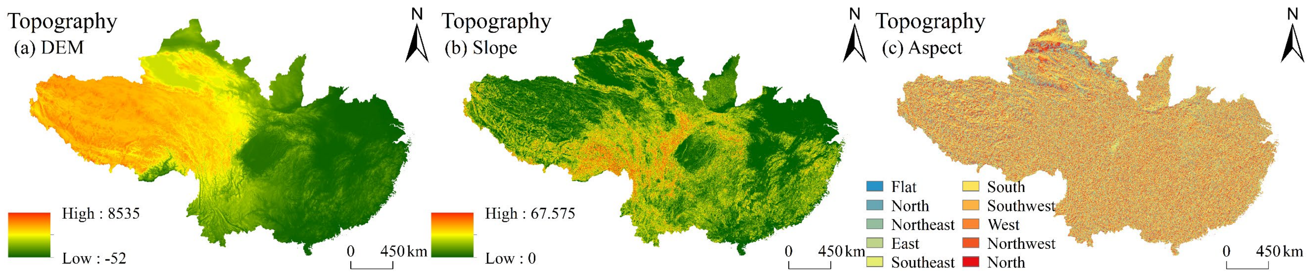
3.1. Ecological Environment Characteristics

Geomorphology–climate–socio-economic factors were analyzed from a geographical perspective. As shown in Figure 3, the DEM value increases from east to west, with the highest DEM value observed in the Tibetan inland flow area and the Yalong River system in the upper reaches of the Yangtze River, and the lowest in the PRB. The basin edge slope value is low, while the slope value of the Yalong River system in the YRB is relatively high. The slope directions are mainly determined as eastward, northeastward, and southward. The climatic and socio-economic factors gradually increase from the west to the east, while the opposite is observed for the DEM (Figure 4). The boundary between Fugu County in Shaanxi Province and Tengchong City in Yunnan Province generally corresponds to the delineation between the ecological and environmental factors. The major urban centers of GDP, POP, and NLD are located in the provincial capitals of Guangzhou, Hangzhou, Changsha, Wuhan, Chengdu, and Kunming, as well as in the central cities of Chongqing and Shanghai, with the coastal cities, CLP, and HAI exhibiting the greatest economic values (Figure 2).

Sen’s slope estimator and the Mann–Kendall test were used to analyze the long-time-series transformations from 2000 to 2020. The results reveal that anthropogenic activities are most clearly manifested in the significant growth rates of NLD, GDP, POP, and HAI (Figure 7). More specifically, the five-year average growth rate of GDP is highly significant at 79.39%. For example, in 2000, the majority of counties with a GDP exceeding 5 × 10⁷ CNY/km² were situated in the lower reaches of the YRB. However, by 2020 (with the exception of some counties in the Yangtze River Delta urban agglomeration), several provincial capitals in the western region, including Changsha, Wuhan, Chengdu, and some neighboring counties, reached a GDP greater than 5 × 10⁷ CNY/km². Changes in population density are most noticeable in and close to major cities such as Guangzhou, Shanghai, Xi’an, Chongqing, and Wuhan, while changes in POP are less pronounced in other cities (e.g., Tibet and Qinghai). Land development is mainly concentrated in the central areas of provincial-level cities and capitals, as well as some prefecture-level cities. In addition, county cities are generally higher compared to boundaries outside the urban agglomerations, indicating their value decreases as they move away from the core cities. TEM exhibits a continuous upward trend, with the most significant increases in the middle and lower reaches of the YRB and the western reaches of the PRB (

Table 8. Trend area ratios of 17 factors from 2000 to 2020.

Area Unit: %	Significantly Increased	Marginally Significantly Increased	Nonsignificantly Increased	No Change	Nonsignificantly Reduced	Marginally Significantly Reduced	Significantly Reduced
WESs	/	+1.70	+59.92	/	−37.01	−1.18	−0.19
WY	+0.04	+3.64	+58.71	0.08	−32.12	−4.23	−0.98
SC	+3.45	+5.81	+44.97	/	−26.34	−12.15	−7.28
NE	+3.04	+5.38	+46.89	0.07	−44.22	−0.40	/
PE	+0.83	+3.51	+54.43	0.07	−39.82	−1.34	/
PRE	+1.11	+5.80	+40.49	0.04	−48.51	−3.45	−0.60
TEM	+28.29	+14.94	+22.86	33.91	/	/	/
EVP	+0.84	+2.33	+71.69	/	−24.70	−0.38	−0.06
RHU	/	+2.36	+48.83	/	−47.72	−1.04	−0.05
NPP	+8.54	+18.75	+62.54	/	−9.15	−1.00	−0.02
NDVI	+14.70	+29.75	+54.73	/	−0.80	/	−0.02
POP	+7.52	+7.42	+49.57	/	−29.92	−5.28	−0.29
NLD	+51.45	+20.22	+7.50	20.75	−0.08	/	/
GDP	+62.40	+20.07	+17.50	0.03	/	/	/
ELP	+0.79	+1.91	+41.94	0.01	−53.45	−1.85	−0.05
CLP	+5.39	+13.81	+55.70	16.99	−7.51	−0.37	−0.23
HAI	+62.40	+20.07	+17.50	0.03	/	/	/

). CLP also presents an increasing trend, accounting for 74.90%, while the opposite is true for ELP, with a decrease of 54.8%. This indicates a significant reduction in vegetation, forest, and water sources. NDVI increased by 99.18%, revealing that most cities have experienced marked greening, with effective ecological protection and restoration.

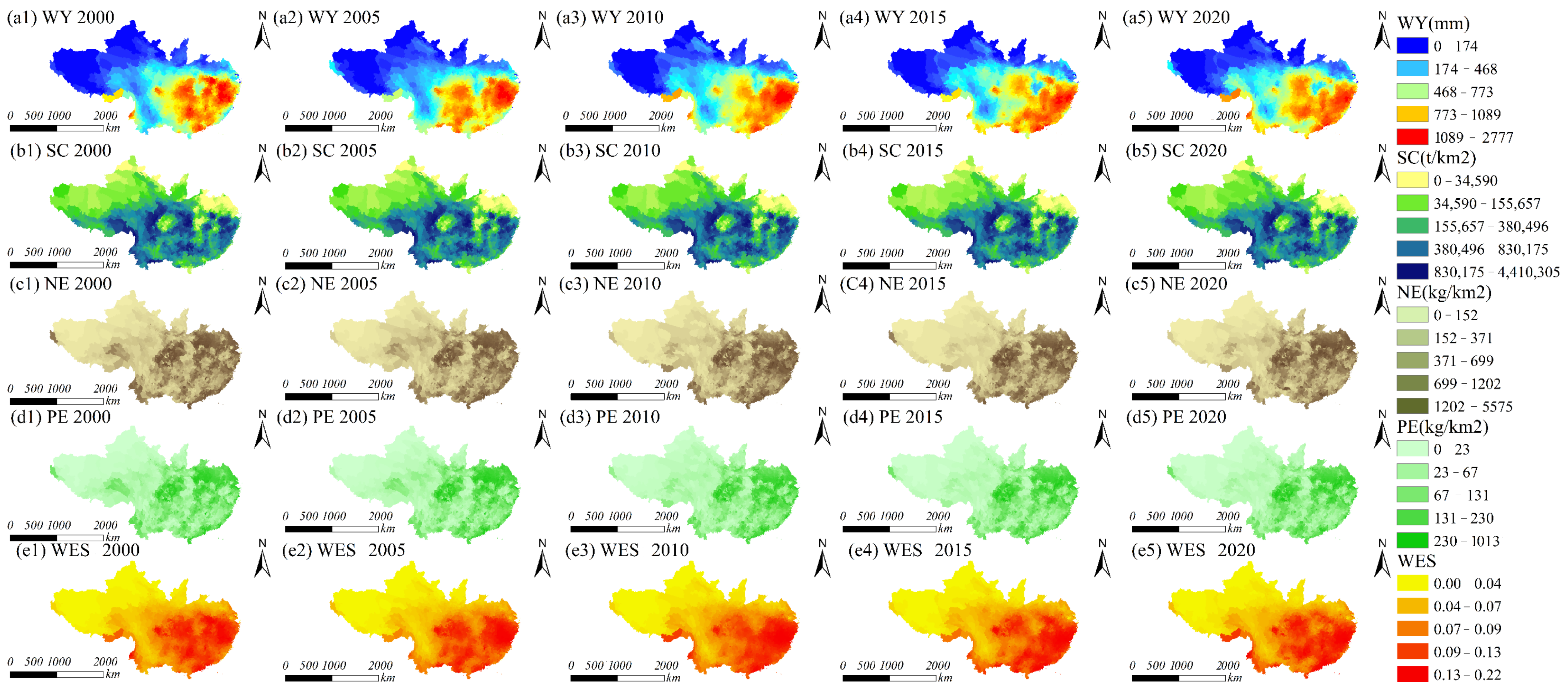
3.2. Spatiotemporal Variation of Multiple WESs

The quantitative assessment of WESs in the study area demonstrates that all four WESs exhibit fluctuating and increasing processes with significant spatial heterogeneity (Figure 8). From 2000 to 2020, WY decreased and subsequently increased, with the total volume changing from 2.20 × 10¹⁴ m³ to 2.39 × 10¹⁴ m³. Moreover, WY increased from the northwest to the southeast, with values in most counties ranging from 300 mm to 800 mm and exhibiting uneven spatial distributions and major regional differences. The highest mean annual precipitation, exceeding 800 mm, was found in the southeastern provinces of Anhui, Fujian, and Jiangxi and their surrounding areas. In contrast, areas in Gansu Province and Tibet exhibited lower annual average water yields, below 300 mm.

SC increased from 2.4473 × 10¹² t to 2.4504 × 10¹² t. Areas with low water quantity and SC values are mainly located in the plains, such as the Sichuan Basin, the Han River Plain, and the Yangtze River Delta Plain. The strongest soil and water conservation capacity values are observed in mountainous counties, such as the Hengduan Mountain area, Qinling–Dabashan Mountain area, Wuling Mountain area, and Zhejiang and Fujian hilly areas, most of which exceed 80,000 t/km².

NE and PE exhibit significant spatial heterogeneity, with large values concentrated in coastal areas and low values in the mountainous regions of Sichuan, Yunnan, and western Hubei. The NE values of most counties in the basin ranged from 150 to 700 kg/km², and total NE increased from 1.5 × 10¹⁰ kg to 1.9 × 10¹⁰ kg between 2000 and 2020. PE generally ranged from 20 to 230 kg/km², and the total PE increased from 2.4 × 10⁹ kg to 3 × 10⁹ kg between 2000 and 2020. The Yangtze River Delta is relatively developed in agriculture and requires the use of large quantities of chemical fertilizers and pesticides, resulting in extreme loads of nitrogen and phosphorus. Urban ecosystems also contribute significantly to the emissions of these elements [69]. Cultivated areas have a significant positive influence on nitrogen loads.

From 2000 to 2020, the average of the WESs increased from 0.0825 to 0.0919. The number of counties with higher WES increases was concentrated in the lower reaches of the basin, with lower numbers in the middle reaches. WESs for the four elements generally exhibited a continuous upward trend, exceeding 50%. This increase is mainly concentrated in the upper reaches of the YRB and the coastal areas.

The overall trend in WESs from 2000 to 2020 can be observed from Sen’s slope analysis and the Mann–Kendall test in Figure 7 and Table 8. The WESs in the upper reaches of the YRB and Hanjiang River system in the PRB showed an upward trend, while the WESs in the middle and lower reaches of the YRB and the Xijiang River system in the PRB exhibited a downward trend. Both NE and PE increased in the middle and lower reaches of the overall south basin, while WY presented an overall decreasing trend.

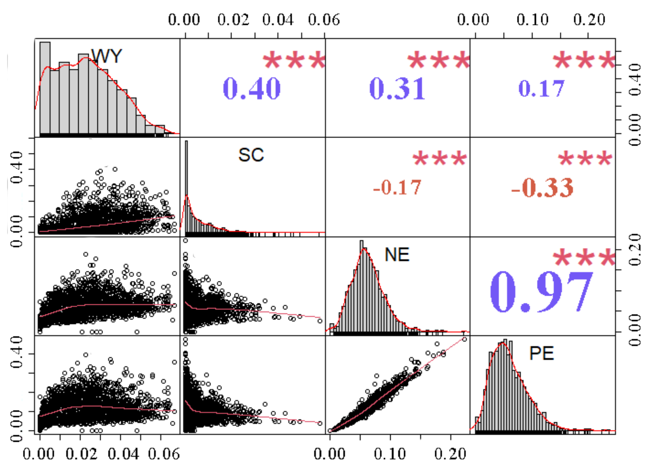
3.3. Relationships between WESs

Due to the non-normal distribution of WESs, we employed Spearman’s correlation to characterize the correlation among grid-level WES changes from 2000 to 2020 (Figure 9). Nitrogen and phosphorus exports exhibited a positive correlation with WY and a negative correlation with SC, suggesting a trade-off between WP and SC. SC is highly positively correlated with WY, which implies a clear synergistic relationship between WP and SC. Consider the redundancy of the data. Despite the high positive correlation between NE and PE, there were significant differences in the correlation values for WY and SC. Therefore, four types of factors can be overlaid to generate WES data using the methodology in Section 2.3.4.

We analyzed the global spatial autocorrelation of WESs (

Table 9. Moran’s I for water-related ecosystem services for the period of 2000–2020.

	2000	2005	2010	2015	2020	2000–2020
Moran’s I	0.69	0.69	0.76	0.68	0.65	0.66
P	0	0	0	0	0	0
Z	148.61	149.00	164.56	146.51	140.42	142.62

) to verify the spatial concentration and dispersion of WESs. The global autocorrelation Moran’s I index was consistently greater than 0 in all periods. This indicates that the spatial distribution of WESs in the ecosystems of the study region was relatively concentrated and that the neighboring regions influenced each other. From 2000 to 2020, Moran’s I index was observed to increase and subsequently decrease.

Figure 10 presents the hot and cold spots of WESs for counties in the study area from 2000 to 2020. A confidence level exceeding 95% (i.e., p < 0.05) is considered statistically significant. Therefore, our analysis focuses on areas with confidence levels greater than 95%. WESs within the study area showed significant hot and cold spot effects. From 2000 to 2020, the hot spots declined from 31.46% to 29.15% of the total area. The hot spots were mainly concentrated in the middle and lower reaches of the basin, with insignificant differences between high and low values. WES cold spots were generally concentrated in the upper reaches of the basin, and the area of cold spots increased from 62.34% to 62.71%.

3.4. Driving Mechanism of the Coupling Coordination Relationship

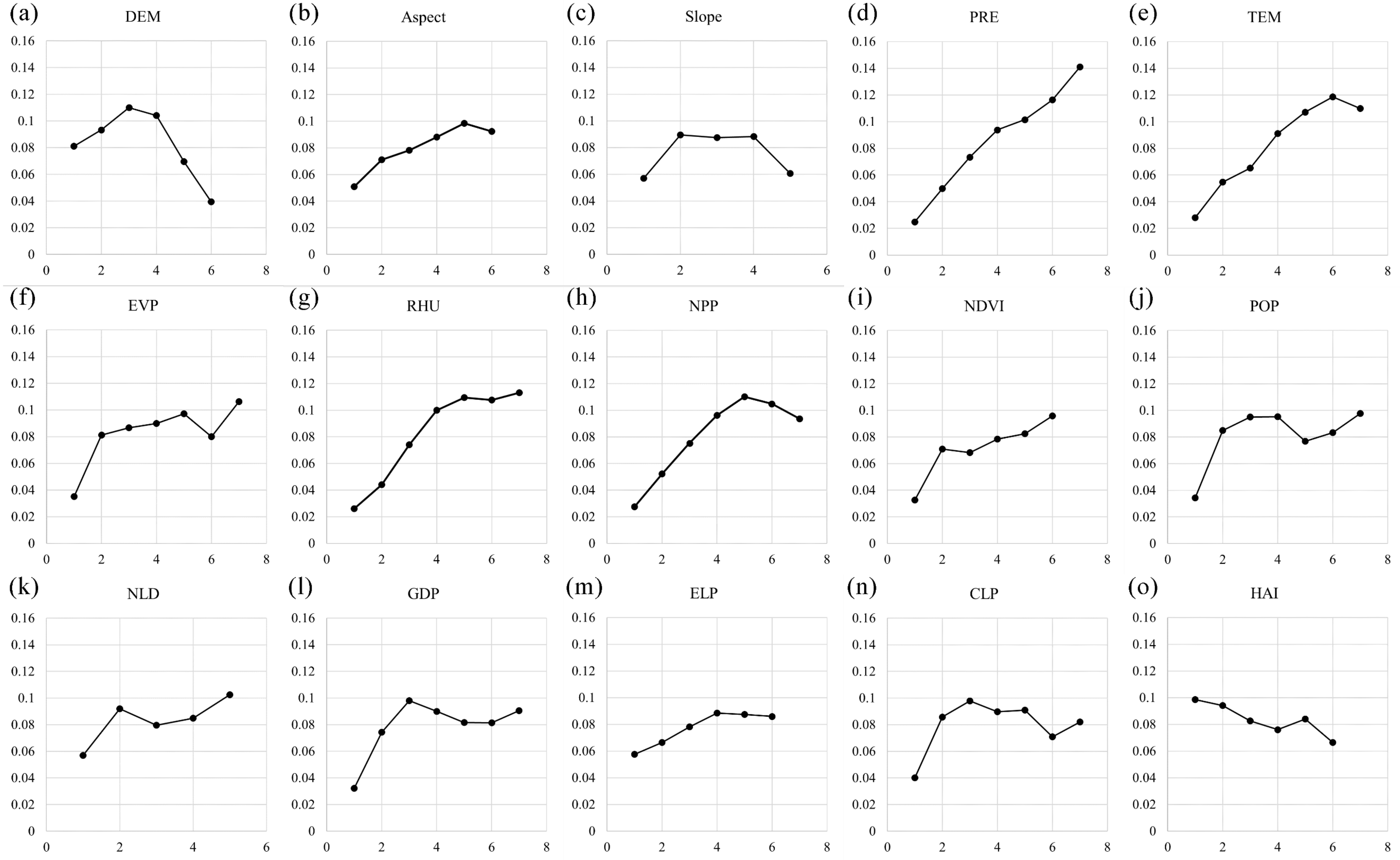
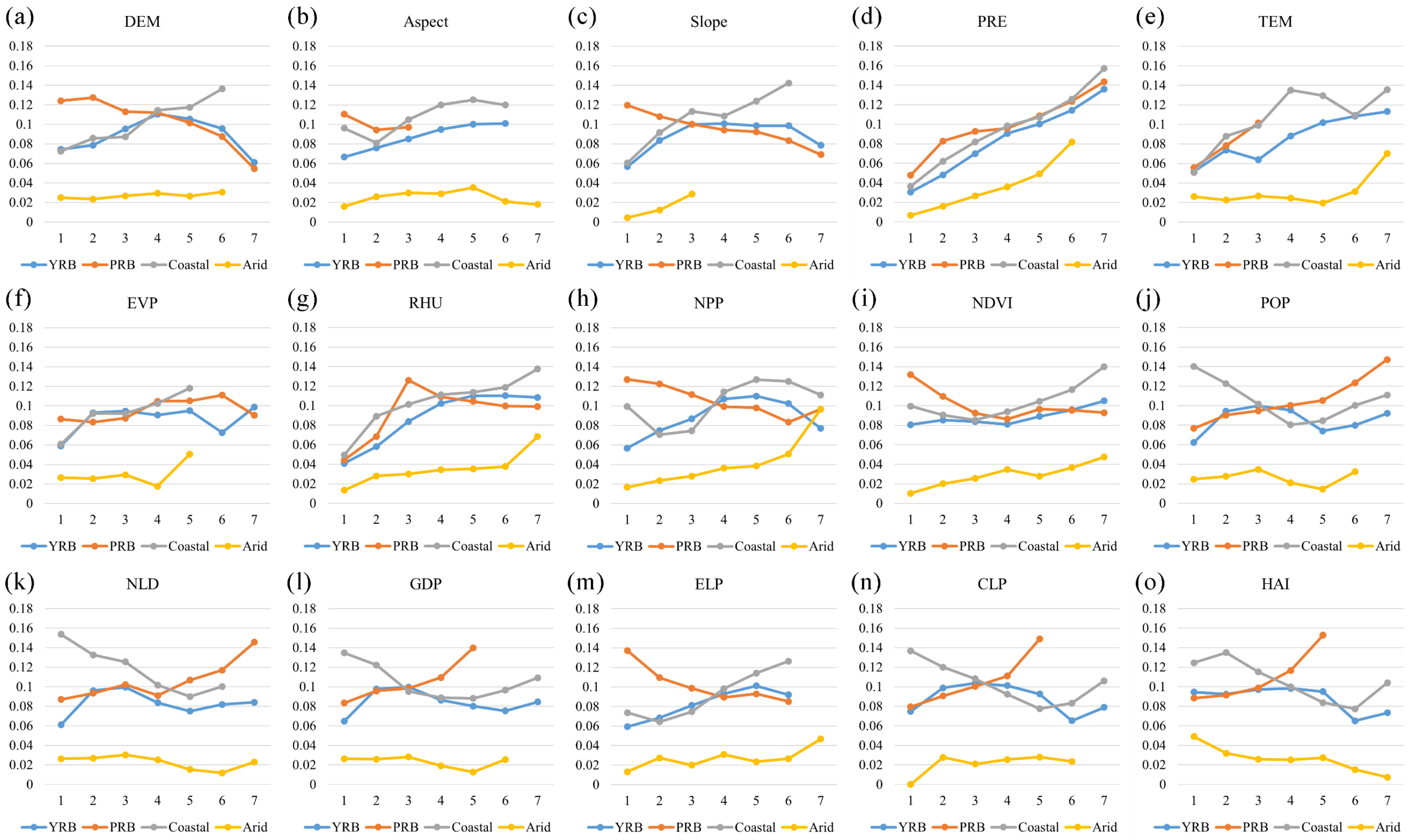
3.4.1. Single-Factor Effect on the Spatial Heterogeneity of WESs

The individual and combined effects of county-level driving factors on WESs were analyzed using the OPGD for the south basin (Figure 11). The effects of each driver on WESs were highly significant (p < 0.001). The q value of each factor reflects its ability to explain the spatial variability of WESs across time. From 2000 to 2020, natural factors such as PRE and TEM play a major role in the spatial differentiation of WESs, with an average explanatory power of 0.4033 and 0.1862, respectively. However, the explanatory power of the natural factors for WESs decreases from 2010 to 2020, with a decreasing value of about 0.07 on average, and the explanatory power of human activities such as POP, GDP, HAI, and NLD for WESs doubles from 2000 to 2010. It can be seen that the natural factor plays a key role from 2000 to 2020, but its explanatory power decreases over time, while the explanatory power of the anthropogenic factor gradually increases over the entire time horizon.

Figure 12 presents the results of the comprehensive analysis of the YRB at different stages of the basin. Over the time span from 2000 to 2020, for the entire YRB, climate factors such as PRE and TEM show the strongest explanatory power in explaining WESs, with an average explanatory power of 0.6178 and 0.1931, respectively. In addition, the explanatory power of climatic factors for WESs gradually increased over time, from the upper to the lower reaches of the YRB. The explanatory power of anthropogenic activities such as POP, GDP, NLD, CLP, and HAI for WESs has been increasing year by year. Among them, anthropogenic activities have the strongest explanatory power for WESs in the lower reaches of the YRB, with an average explanatory power of 0.3906. Compared with the period from 2000 to 2010, this explanatory power has increased by 0.1818, which is 0.0979 more than the increase in the value of natural factors. Therefore, the explanatory power of anthropogenic activities has shown a tendency of the lower reaches of the YRB > the upper reaches of the YRB > the middle reaches of the YRB. DEM and slope dominated the explanatory power of WESs, especially in the lower reaches of the YRB, with an average explanatory power of 0.586. The LULC factors, such as CLP and ELP, had a significant impact on WESs in the YRB, especially in the lower reaches of the YRB.

Figure 13 presents the results of the combined analysis for different basins in the south basin. For the YRB and SCR, climate factors show the strongest explanatory power in explaining WESs, with an average explanatory power of 0.4055 and 0.5776, respectively. The explanatory power of anthropogenic activities for different watersheds increases between 2000 and 2020. Geomorphology and LULC type play an important role in all southern basins, having the strongest explanatory power in the SCR.

3.4.2. Influence of LULC on the WESs

The influence of LULC change on WES supply has been commonly reported [70]. To further validate the effect of LULC on WESs, we analyze the change in WES hot and cold spots from 2000 to 2020 by dividing them into two types of regions, high WESs and low WESs, superimposed on the LULC type. The LULC change characteristics in the southern basins reveal construction land as the only LULC type to exhibit a significant increase, with the largest areas corresponding to those with high levels of WES change (Figure 14). The rise in construction land will cause serious human interference with the natural ecosystem and place the habitats of numerous organisms at risk [71]. The widespread damage to natural ecosystems will enhance this phenomenon. Among the zoning types, cropland has exhibited the greatest reduction in area and has been seriously affected by construction land. Therefore, WES changes in food production are also seriously affected by WESs. As the changes in WESs increase, water body areas decline, and the flood control ability of the basin also decreases [72]. For areas with high-level WESs, all LULC types (with the exception of forest land) are converted to construction land. WES change resulted in the largest increase in forest area in lower-class areas. This reciprocal conversion of natural vegetation may weaken the effects of changes in WES demand. The results once again validate that the effects of human activities are gradually outweighing the effects of natural change.

3.4.3. Nonlinear Effects of Factors

As shown in Figure 15, the results of the risk detector analysis allow for the determination of the nonlinear response of changes in specific factor levels to changes in WESs. For example, the effect of precipitation on WESs shows a gradual increase in the service increase of WESs as PRE increases, peaking at level 7 (500 mm–519 mm) at 0.14. TEM shows a similar trend to PRE but begins to decline after reaching the peak at level 6 (16.8–17.5 °C). In addition, DEM gradually had a negative effect on WESs after exceeding the third order (4226 m). This suggests that within a certain range, elevation may have a positive effect on WESs, but exceeding a certain threshold may lead to negative effects. The effect of slope on WESs showed an optimum below 19°, and it was not the case that flatter terrain was more favorable for WESs. This suggests that within a certain range of slopes, moderate variations in terrain may be more favorable for WES provision.

The trend of RHU was consistent with those of PRE, TEM, and NDVI. WES growth rates were higher on shaded and semi-shaded slopes (north slopes) than on sunny and semi-sunny slopes (south slopes). Shaded and semi-shaded slopes have a weaker evapotranspiration capacity and a stronger water storage capacity than sunny and semi-sunny slopes, thus enhancing WESs, particularly in arid areas. The growth rate of WESs decreased in areas with higher GDP, CLP, and HAI. However, the highest WES values were observed in densely populated areas with the largest NLD.

Figure 16 presents the results of the comprehensive analysis of the YRB at different stages of the basin. The results of the analysis show that WESs increase with the continuous increase in PRE levels. TEM exhibits similar characteristics to PRE in all basins, with the difference being in the upper reaches of the YRB, which peaks at 0.102 at level 6 (17.28–18.67 °C) with increasing TEM and then gradually decreases to 0.086 at level 7. A certain level of elevation and slope increase does not negatively affect WESs, but in the lower YRB, higher DEMs and slopes favor WESs. Aspect has similar results to the analyses throughout the southern basins. For human activities such as POP, GDP, NLD, and HAI, the impact on WESs is not linear. The impacts are not more favorable with higher values, but above a certain peak, they can have a negative impact on WESs.

In order to verify that different basins have different degrees and trends of factors, we performed factor analysis for the YRB, PRB, IFA, and SCR. Figure 17 presents the results in the YRB. WESs increased with PRE, TEM, and EVP. The trend of RHU was consistent with that of the climatic factors, with an optimal range of 77.61–79.58%. However, the increase in anthropogenic activities was detrimental to the WESs, and the median value was observed as most favorable for aquatic ecosystems. In the PRB, WESs increased with PRE, TEM, POP, NLD, GDP, CLP, and HAI. Moreover, WESs were most favorable when NPP, slope, NDVI, and ELP reached their minimum values. Higher DEM and slope values in the IFA were more favorable for WESs, unlike in the YRB and PRB, which were consistent with the SCR. WESs increased with PRE, TEM, EVP, RHU, NPP, ELP, and NDVI. However, in the SCR, WESs are most favorable when the NPP is in the middle of the range (642.48–792.31 g/m²·a¹). The trends in the anthropogenic activities within the SCR are consistent with those in the YRB, and the lower the frequency of anthropogenic activities, the more favorable the WESs.

By analyzing the nonlinear effects of various factors on WESs at different geographical locations in the same basin and in different basins, it can be found that climatic factors, such as PRE and TEM, show a tendency to enhance their effects on WESs as they increase. However, for different regions, higher TEMs are not more favorable to WESs, suggesting that their effects may be moderated by factors such as geographic location. Socio-economic and anthropogenic factors are more favorable to WESs within a certain threshold and may negatively affect WESs beyond this threshold. This suggests that there is a need to balance the impacts of climatic and socio-economic–anthropogenic factors when managing and conserving WESs, with particular attention to the nonlinear relationship between these factors. These findings of nonlinear responses provide insights into the relationship between factors and WESs, which can contribute to more effective ecosystem management strategies and sustainable development programs.

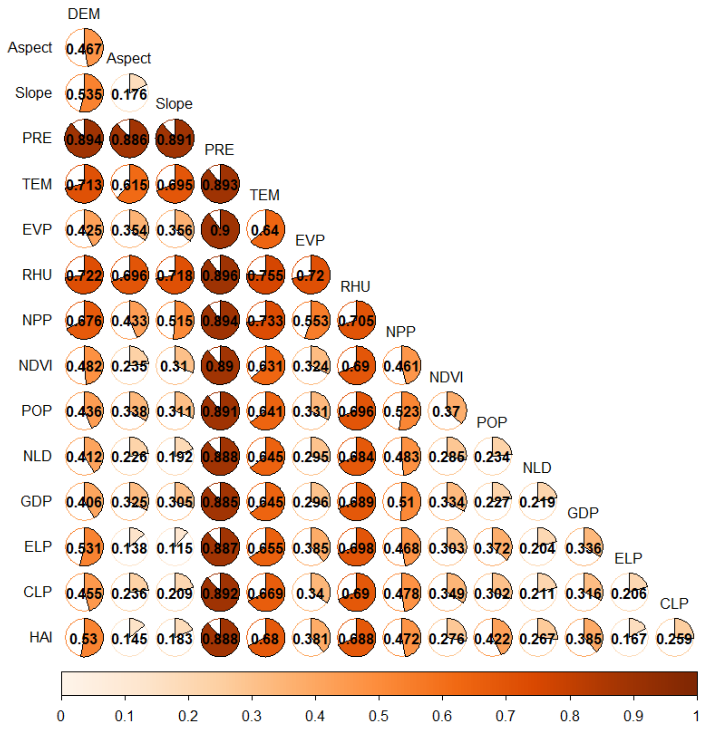
3.4.4. Interaction between Factors Influencing the Spatial Heterogeneity of WESs

To further investigate the influence of two-dimensional factors on the spatial heterogeneity of WESs, this study used an interaction detector to reveal the interaction between two drivers. The interaction between any two drivers exhibited either a two-way enhancement or a nonlinear enhancement in the explanatory power of the WES spatial heterogeneity. Detailed analyses of the entire basin revealed the three interaction factors exerting the strongest effect on the spatial heterogeneity of WESs to be PRE ∩ EVP, PRE ∩ RHU, and PRE∩TEM, with explanatory coefficients of 0.8997, 0.8962, and 0.8926, respectively (where ∩ denotes the interaction between different socio-economic factors). TEM ∩ HAI, TEM ∩ CLP, and TEM ∩ GDP exert the strongest nonlinear enhancement of spatial heterogeneity in WESs, with explanatory powers exceeding 0.64. The interaction of climate factors (PRE, TEM, and RHU) is observed to play a dominant role in WESs (Figure 18). Moreover, anthropogenic impacts rapidly affect ecosystems by influencing surface vegetation and soil conditions. Human-induced urbanization and socio-economic activities interacted with climate factors to influence WESs, suggesting that the joint impacts of multiple drivers exceed those of the joint effects of a single factor. HAI follows an increasing bifactorial trend under the influence of PRE and RHU and increases nonlinearly when interacting with other factors. The effects of each driving factor on the spatial differentiation of WESs are not independent but interact with each other, and the explanatory power of the interaction of all factors is stronger than that of a single factor, presenting a nonlinear enhancement or two-factor enhancement relationship. The spatial differentiation of WESs is affected by both natural and anthropogenic factors. In particular, when anthropogenic factors are combined with natural factors, the influence on WESs is significantly enhanced.

We analyzed the effects of the interactions between the two-dimensional drivers on WESs in different basins.

Table 10. The impact of interactions between pairs of factors in the Yangtze River Basin.

Variable	DEM	Aspect	Slope	PRE	TEM	EVP	RHU	NPP	NDVI	POP	NLD	GDP	ELP	CLP
Aspect	0.4736
Slope	0.5462	0.4956
PRE	0.8746	0.8701	0.8792
TEM	0.7693	0.5927	0.7888	0.8632
EVP	0.5091	0.3389	0.5704	0.8605	0.5244
RHU	0.5271	0.4645	0.5683	0.8871	0.6403	0.4899
NPP	0.5431	0.4395	0.5389	0.8915	0.6883	0.5082	0.4771
NDVI	0.4992	0.3828	0.5444	0.8674	0.7501	0.4399	0.4414	0.5295
POP	0.5238	0.4195	0.5457	0.8845	0.7258	0.4061	0.4887	0.5426	0.3877
NLD	0.5073	0.3794	0.5236	0.8657	0.6785	0.3428	0.3738	0.4769	0.3216	0.3206
GDP	0.5054	0.3871	0.5431	0.8832	0.7204	0.3536	0.4315	0.5198	0.3347	0.3238	0.2237
ELP	0.4817	0.4510	0.5087	0.8821	0.6601	0.5121	0.4108	0.4722	0.5128	0.5247	0.4512	0.4951
CLP	0.5105	0.4448	0.5439	0.8931	0.7332	0.4622	0.4703	0.4960	0.4062	0.4400	0.3890	0.3960	0.4762
HAI	0.4748	0.4435	0.5229	0.8960	0.7083	0.4627	0.4384	0.4601	0.4800	0.5265	0.4149	0.4579	0.4302	0.4027

presents the results for the YRB. The interaction factors with the strongest effect on the spatial heterogeneity of WESs are PRE ∩ HAI, PRE ∩ CLP, and PRE ∩ NPP.

Table 11. The impact of interactions between pairs of factors in the Pearl River Basin.

Variable	DEM	Aspect	Slope	PRE	TEM	EVP	RHU	NPP	NDVI	POP	NLD	GDP	ELP	CLP
Aspect	0.5829
Slope	0.5780	0.2577
PRE	0.8434	0.8432	0.8498
TEM	0.6048	0.3464	0.4084	0.8471
EVP	0.6943	0.1742	0.4676	0.8781	0.4363
RHU	0.7299	0.5744	0.6811	0.8770	0.6814	0.6842
NPP	0.6319	0.1577	0.3342	0.8842	0.4283	0.3856	0.6298
NDVI	0.6491	0.2085	0.3660	0.8660	0.4090	0.4461	0.6930	0.2205
POP	0.6531	0.2831	0.3542	0.8851	0.4566	0.4860	0.6866	0.3617	0.3516
NLD	0.6654	0.2776	0.3590	0.8676	0.4397	0.4851	0.6898	0.3390	0.3168	0.2899
GDP	0.6423	0.2791	0.3458	0.8614	0.4445	0.4425	0.6896	0.3206	0.3514	0.2729	0.2695
ELP	0.6258	0.2283	0.2872	0.8799	0.3996	0.3974	0.6705	0.2587	0.3370	0.3110	0.2919	0.2971
CLP	0.6611	0.3133	0.3376	0.8724	0.5020	0.4709	0.7244	0.3484	0.3920	0.3095	0.3124	0.2952	0.3386
HAI	0.6587	0.2620	0.3390	0.8887	0.4238	0.3823	0.6819	0.2981	0.3530	0.3196	0.3022	0.2946	0.2851	0.3145

presents the results from the PRB, revealing PRE ∩ HAI, PRE ∩ POP, and PRE ∩ NPP to have the greatest effect on the spatial heterogeneity of WESs.

Table 12. The impact of interactions between pairs of factors in Inward Flowing Area.

Variable	DEM	Aspect	Slope	PRE	TEM	EVP	RHU	NPP	NDVI	POP	NLD	GDP	ELP	CLP
Aspect	0.4736
Slope	0.5462	0.4956
PRE	0.8746	0.8701	0.8792
TEM	0.7693	0.5927	0.7888	0.8632
EVP	0.5091	0.3389	0.5704	0.8605	0.5244
RHU	0.5271	0.4645	0.5683	0.8871	0.6403	0.4599
NPP	0.5431	0.4395	0.5389	0.8915	0.6883	0.5082	0.4771
NDVI	0.4992	0.3828	0.5444	0.8674	0.7501	0.4399	0.4414	0.5295
POP	0.5238	0.4195	0.5457	0.8845	0.7258	0.4061	0.4887	0.5426	0.3877
NLD	0.5073	0.3784	0.5236	0.8657	0.6785	0.3428	0.3738	0.4769	0.3216	0.3206
GDP	0.5054	0.3871	0.5431	0.8832	0.7204	0.3536	0.4315	0.5198	0.3347	0.3238	0.2237
ELP	0.4817	0.4510	0.5087	0.8821	0.6601	0.5121	0.4108	0.4722	0.5128	0.5247	0.4512	0.4951
CLP	0.5105	0.4448	0.5439	0.8931	0.7332	0.4622	0.4703	0.4960	0.4062	0.4400	0.3890	0.3960	0.4762
HAI	0.4745	0.4435	0.5229	0.8960	0.7083	0.4627	0.4384	0.4601	0.4800	0.5265	0.4149	0.4579	0.4302	0.4027

and

Table 13. The impact of interactions between pairs of factors in Southeast Coastal River Basin.

Variable	DEM	Aspect	Slope	PRE	TEM	EVP	RHU	NPP	NDVI	POP	NLD	GDP	ELP	CLP
Aspect	0.4736
Slope	0.5462	0.4956
PRE	0.8746	0.8701	0.8792
TEM	0.7693	0.5927	0.7888	0.8632
EVP	0.5091	0.3389	0.5704	0.8605	0.5244
RHU	0.5271	0.4645	0.5683	0.8871	0.6403	0.4899
NPP	0.5431	0.4395	0.5389	0.8915	0.6883	0.5082	0.4771
NDVI	0.4992	0.3828	0.5444	0.8674	0.7501	0.4399	0.4414	0.5295
POP	0.5238	0.4195	0.5457	0.8845	0.7258	0.4061	0.4887	0.5426	0.3877
NLD	0.5073	0.3794	0.5236	0.8657	0.6785	0.3428	0.3738	0.4769	0.3216	0.3206
GDP	0.5054	0.3871	0.5431	0.8832	0.7204	0.3536	0.4315	0.5198	0.3347	0.3238	0.2237
ELP	0.4817	0.4510	0.5087	0.8821	0.6601	0.5121	0.4108	0.4722	0.5128	0.5247	0.4512	0.4951
CLP	0.5105	0.4448	0.5439	0.8931	0.7332	0.4622	0.4703	0.4960	0.4062	0.4400	0.3890	0.3960	0.4762
HAI	0.4748	0.4435	0.5229	0.8960	0.7083	0.4627	0.4384	0.4601	0.4800	0.5265	0.4149	0.4579	0.4302	0.4027

present the results for the IFA and SCR, respectively. The three interaction factors with the greatest influence on the spatial heterogeneity of WESs for these basins are identified as PRE ∩ HAI, PRE ∩ CLP, and PRE ∩ RHU. The above analysis indicates that the combined effect of human activities and climate is greater than the combined effect of other factors, and the combined effect of climate and other factors is significantly larger than the interaction effect of other factors.

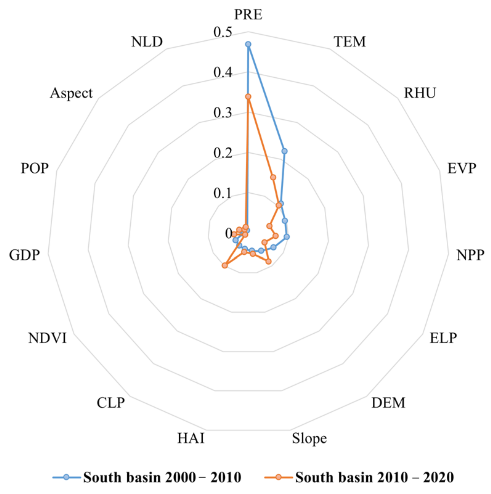
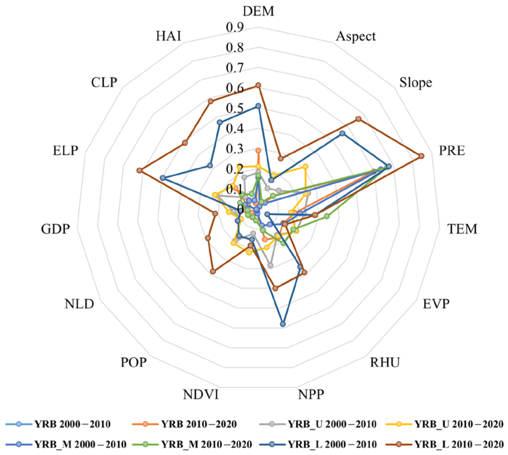
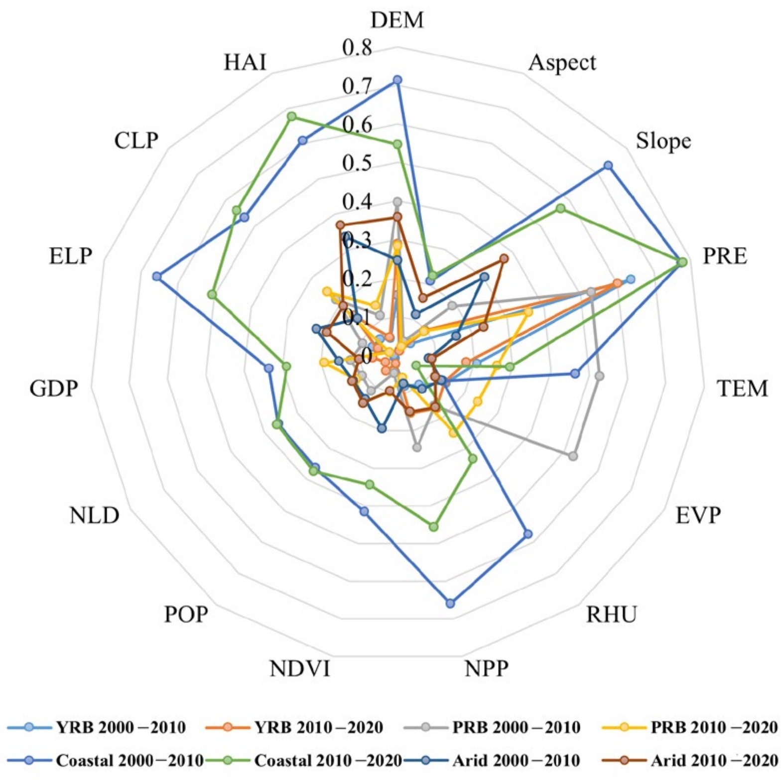
3.4.5. Spatial Characteristics of Factors Influencing WESs

To reveal regional differences in the effects of drivers on WESs, spatial interactions between WESs and factors were analyzed using MGWR. The VIF values of the selected drivers were all below 10, indicating low multicollinearity.

Table 14. Factor detection results on the coupling coordination degree in the south basin.

Model Parameter	Multiple R-Squared (R2)	Adjusted R-Squared (Adjusted R2)	Akaike Information Criterion (AICc)
OLS	0.944	0.943	6830.725
GWR	0.984	0.981	1950.940
MGWR	0.989	0.986	1730.905

compares the MGWR, GWR, and OLS results. The AICc (Akaike Information Criterion corrected) value of MGWR is 1730.905, which is lower than that of OLS and GWR. In addition, the R² and adjusted R² values of MGWR are 0.989 and 0.986, respectively, which are significantly higher than those of OLS and GWR, demonstrating the superior fit of MGWR. The results show that MGWR can reveal the heterogeneous impacts of drivers on WESs in different regions and explain the spatial relationship between drivers and WESs better than the other models.

Figure 19 presents the regression coefficients of different geographical location factors derived from MGWR, while

Table 15. Joint effects of drivers on water-related ecosystem services.

	DEM	Aspect	Slope	PRE	TEM	EVP	RHU	NPP	NDVI	POP	NLD	GDP	ELP	CLP	HAI
MRC	0.681	0.02	0.185	1.111	0.973	−0.045	0.355	−0.035	0.007	0.061	0.074	0.001	0.11	0.069	0.141

reports the average regression coefficients. The key factors affecting WESs vary with the spatial location. PRE promotes WESs in all regions, particularly in Jiangsu Province, Yunnan Province, and other regions. Factors such as DEM inhibit WESs in the middle and upper reaches of the basin. TEM has a positive impact on WESs in Anhui, Jiangsu, and Guangdong provinces, and an inhibitory effect on WESs in Hubei, Guizhou, and Guangxi provinces. Overall, natural factors exert a positive impact on much of the basin. However, when POP, NLD, GDP, CLP, and HAI are considered, it is clear that increased human activities have a greater inhibitory effect on WESs. The human exploitation of ecosystems increases with the population density. Since ecosystems are rooted in the natural environment, the positive effects of natural factors determine the spatial trends of the ecosystem.

In summary, spatial differences in natural factors result in the spatial heterogeneity of ecosystems. Compared to natural factors, anthropogenic factors dominate the negative impacts in most parts of the basin. LULC change is the main indicator of anthropogenic factors and exerts a strong influence in fields such as urban agglomerations and afforestation.

4. Discussion

4.1. Impact of Human and Natural Factors on WESs

At the global scale, the OPGD and MGWR models confirm that natural factors are the primary influencers of WESs. The results of single-factor detection show that natural factors such as PRE (0.4032) and TEM (0.1862) have the strongest driving force on the spatiotemporal differentiation of WESs in the southern basins, which is consistent with previous studies that have identified PRE and TEM as the main drivers of spatiotemporal differentiation of regional WESs [24]. Bai et al. [73] demonstrated that PRE directly influences water input and surface hydrological processes. The WESs in the southern part of the southern watershed are more sensitive to PRE, and their spatial distribution changes synchronously with PRE. Compared with the impacts of globally induced WESs, the effects of local WESs exhibit slight differences. When analyzing sub-basins, it was found that the HAI (0.3518) in IFA had the strongest driving force on the spatiotemporal analysis of WESs. IFA, as a special geographical unit in the southern basins of China, has a large area of natural surfaces, with widespread deserts and Gobi beaches and low rainfall [74]. Therefore, natural factors represented by PRE do not have a strong driving force on the spatiotemporal distribution of WESs in IFA. Human activities can mitigate WESs by increasing the water supply or changing LULC [75]. This finding is consistent with Fang et al.’s [24] research conclusion, taking into account the low rainfall, the impact of human activities on the surface, and the influence of regional ecosystems by biophysical and biogeochemical mechanisms. Consequently, the changes in WESs caused by human activities are more pronounced than those caused by natural factors. Simultaneously, through comparisons over the years, it has been observed that the impact of human factors on WESs grows over time, which is consistent with the viewpoint expounded by Li et al. [76]. The increase in urban impervious surfaces will affect surface runoff and sediment transport, leading to abnormal changes in WY and SC. Accompanied by urbanization, population growth requires more WESs, placing significant pressure on ecosystems. For example, Su et al. [77] demonstrated that the WES value in Shanghai decreased in tandem with economic and population growth. As urbanization accelerated, the rate of decline in the WES value was faster in areas proximal to the city center.

We observed an interesting pattern that PRE gradients play a key role in determining the importance of environmental and anthropogenic factors for WESs in our study area. The q statistics of anthropogenic factors such as LULC type (CLP, HAI), POP, and NLD are significantly higher at lower PRE levels (e.g., at level 1), suggesting that changes in WESs are mainly influenced by human activities. This situation explains the characteristics of WESs’ impact in IFA. Liu et al. [78] have also demonstrated this point. The q statistics of natural factors, such as TEM and DEM, increase significantly when rainfall reaches the second to the fifth stage, and anthropogenic factors begin to decline after reaching a certain peak. At this point, human activities and natural factors jointly influence WESs. When PRE reaches stage 6, the q values of PRE and TEM are significantly higher than other drivers, while the q statistics of LULC types are smaller, indicating that changes in WESs are mainly influenced by natural factors. This view is the same as the conclusion of Li et al. [76].

Our study showed that the effects of various influences on WESs showed nonlinear variations. WESs increased with increasing PRE, which is consistent with the results of previous studies [24]. The effect of TEM on WESs reached a peak of 0.12 in stage 6, after which it began to slow down the effect on WESs. The negative impacts of human factors, such as HAI, on WESs are effective within a certain range. Interactions between different impact factors tend to enhance their combined effects on WESs. The effects of aspect, NDVI, and EVP on WESs are not well behaved at different times, but the interaction with climatic factors such as PRE and TEM can enhance their explanatory power. For example, the synergistic effect of TEM factors with PRE is significantly stronger than the synergistic effect of individual factors (TEM ∩ PRE = 0.893 > TEM). We also observe that interactions between human activities and natural conditions influence changes in WESs (PRE ∩ POP = 0.891 > POP, TEM ∩ POP = 0.641 > POP). These interactions typically amplify the effects of human activities. This conclusion is consistent with the views of Li et al. [76].

Compared to OLS and GWR, the MGWR regression model can reveal the impact of dominant driving factors on WESs with more accurate spatial display information. The MGWR coefficients illustrate the spatial heterogeneity associations between the finally selected driving factors of WESs, providing valuable guidance for local ecological planning and playing a significant role in promoting the spatial coordination of the regional ecological environment’s natural supply and social demand.

The study found that human factors have a negative impact on WESs in basins. This phenomenon indicates that the higher the intensity of human activity, the more unfavorable it is for WESs. Human activities can promote WES supply through soil and water conservation measures such as afforestation [77]. Therefore, it is necessary to strictly limit human interference, rationally allocate basin land resources, further optimize LULC structure, and improve LULC efficiency. For example, some idle land within and around cities can be converted into green spaces. The topographic slope has both positive and negative impacts on WESs. The high coefficients are mainly distributed in the YRB and SCR, which may be closely related to the complex impact of topographic fluctuations on WESs. Geomorphological conditions regulate the spatial pattern of ecosystem supply and demand coordination by affecting the natural supply and social demand of ecosystems. For example, elevation and slope can directly affect soil type, humidity, temperature, evapotranspiration, and other biophysical conditions, ultimately leading to a spatially heterogeneous pattern of WESs [78]. PRE has a positive impact on WESs, and previous studies have also demonstrated the significant and positive effects of precipitation on WESs [30]. Overall, the positive effect of PRE on WESs gradually weakens from east to west. Considering the above research results, a series of spatially specific and targeted ecological protection measures can be adopted. For example, water-saving and drought-resistant plants can be planted in IFA, which can not only improve WESs but also meet humans’ needs for rest areas.

4.2. Policy Impacts

Economic strategies and ecological protections should consider the environmental carrying capacity and economic growth trends across regions. Throughout the basin, an increasing amount of land is being used for urban development while the supply of water resources is simultaneously diminishing. The natural environment has gradually become overloaded by the continuously growing population, while water scarcity has become the soft underbelly of the basin’s development. Moreover, although urbanization has promoted economic growth, it has also induced environmental problems. Pollution emissions and ecological LULC are the principal factors causing regional ecosystem destruction [76]. Conversely, environmental problems due to ecological degradation can also hinder urban development to some extent [79]. The results suggest that although human factors can affect the sustainability of WESs, natural factors are the dominant driving force of the spatial trends in basin ecosystems. The development of megacities has had a negative impact on ecosystems and has increased environmental pressure. Therefore, the future development of the basin should prioritize the protection of the natural environment, for example, maintaining land restoration projects such as “converting farmland into forests” in key areas and extensively promoting green development. Environmental protection should focus on the balanced growth of nature, society, and the economy; the establishment of an eco-friendly socio-economic structure that is beneficial to the public interest; and sustainable development, in which the economy and the natural environment harmoniously coexist.

4.3. Comparisons with Previous Studies

Compared to previous studies on WESs in southern watersheds in China, the notable feature of this study lies in its verification and generalization of the impact mechanisms of WESs in four different regions of a southern watershed using long-term multi-remote sensing image data. Through this approach, this study reveals the factors affecting the evolution of WESs and their spatial heterogeneity, providing a scientific basis for implementing differentiated ecological protection measures. Furthermore, considering the shortcomings of previous studies in exploring the spatial heterogeneity of the impact of driving factors on WESs, this study uses the MGWR model to reveal the impact of dominant driving factors on WESs with more accurate spatial display information, thereby deepening the understanding of the driving factors of watersheds with different characteristics.

Compared to existing WES research, the greatest innovation of this study lies in its strong comparability, adaptability, transferability, intuitiveness, and non-subjectivity, which enable this study to systematically explore the evolution and driving mechanisms of macro and local WESs. Firstly, unlike traditional subjective methods of selecting WES elements, this study selects the elements that make up WESs based on information from literature analysis (Section 2.3.1), which has high objectivity and scientificity, forming a solid foundation for this study. Secondly, the validity of previous WES assessment results is often difficult to verify. Considering the comparability of this research method, through long-term sequential changes and multi-regional comparisons, we observe that natural and human factors have varying degrees of impact on WESs at different times and spatial scales. Thirdly, the OPGD selects the combination of classification parameters with the highest q value to discretize continuous variables, enhancing the quantitative research on the driving mechanism of WESs while overcoming human subjectivity. Fourthly, the MGWR method used in this study helps to intuitively demonstrate the impact of driving factors on WESs at different spatial scales. Finally, the method framework of this study shows strong adaptability and portability. We have demonstrated that OPGD and MGWR can be adapted to WES analysis in other research fields.

4.4. Limitations and Prospects

Despite the great progress made by this study, it is associated with several limitations. For example, the study area covers 55.88% of China’s provinces, with diverse topography, climate zones, and vegetation types. Typical ecosystems may not fully represent the overall ecological conditions of all basins. Therefore, we analyzed the YRB, PRB, IFA, and SCR. However, when quantifying WESs, the weight of the indicator directly affects the results. Our adoption of the equal weighting method may not effectively account for this, and uncertainties still exist. With economic development and social progress, the willingness and ability to serve the ecosystem will increase. Therefore, WES research should be more informative and better reflect socio-economic–ecological trade-offs. Multiple methods should be used to quantify the supply of each WES.

5. Conclusions

This study offers a comprehensive spatial evaluation of WESs, thereby enhancing our understanding of the impacts and spatial characterization of natural and human factors on these services. In this study, based on long-time-series multi-remote sensing data, we use the OPGD and MGWR frameworks to explore the multiple influences on WESs in different sub-watersheds of a watershed and compare regional differences based on scientific assumptions. The results demonstrate that: at the entire basin scale, 61.62% of the counties within the basin showed an increasing trend in WESs over time. From 2000 to 2020, WY initially decreased before rising again, with a total volume increase of 1.9 × 10¹³ m³; SC increased by 3.1 × 10⁹ t; NE increased by 0.4 × 10¹⁰ kg; and PE increased by 0.6 × 10⁹ kg. Through a comparative analysis of long-term driving factors, changes in natural factors, especially PRE, were found to have a more critical impact on WESs than human factors. However, as construction areas expand, the impact of construction areas on WESs gradually increases. For different sub-basins, the factors affecting WESs and their degrees of influence vary. HAI is the primary factor affecting WESs in IFA, while PRE is the main factor affecting WESs in other sub-basins. Both the entire basin and sub-basins exhibit a characteristic where the explanatory power of a single factor tends to increase when interacting with other factors. Furthermore, the response of WES changes to influencing factors is often nonlinear. Natural factors play a positive role in the southern basins, weakening from east to west, while human factors have a negative impact, particularly in densely populated areas, with spatially uneven distribution. The research findings indicate that integrating multi-remote sensing data with OPGD and MGWR models based on a long time series is an effective approach to addressing the driving factors of WESs in complex regions.

References

1. Costanza, R.; d’Arge, R.; De Groot, R.; Farber, S.; Grasso, M.; Hannon, B.; Limburg, K.; Naeem, S.; O‘neill, R.V.; Paruelo, J.; et al. The value of the world‘s ecosystem services and natural capital. Nature 1997, 387, 253–260. [Google Scholar] [CrossRef]
2. Deng, X.; Li, Z.; Gibson, J. A review on trade-off analysis of ecosystem services for sustainable land-use management. J. Geogr. Sci. 2016, 26, 953–968. [Google Scholar] [CrossRef]
3. Zhan, J.; Zhang, F.; Chu, X.; Liu, W.; Zhang, Y. Ecosystem services assessment based on emergy accounting in Chongming Island, Eastern China. Ecol. Indic. 2019, 105, 464–473. [Google Scholar] [CrossRef]
4. Burkhard, B.; Kroll, F.; Nedkov, S.; Müller, F. Mapping ecosystem service supply, demand and budgets. Ecol. Indic. 2012, 21, 17–29. [Google Scholar] [CrossRef]
5. Harris, J. Millennium Ecosystem Assessment; Cranfield University: Cranfield, UK, 2001. [Google Scholar]
6. Li, Z.; Xia, J.; Deng, X.; Yan, H. Multilevel modelling of impacts of human and natural factors on ecosystem services change in an oasis, Northwest China. Resour. Conserv. Recycl. 2021, 169, 105474. [Google Scholar] [CrossRef]
7. Shi, P.; Li, Z.; Li, P.; Zhang, Y.; Li, B. Trade-offs among ecosystem services after vegetation restoration in China’s Loess Plateau. Nat. Resour. Res. 2021, 30, 2703–2713. [Google Scholar] [CrossRef]
8. Fu, Q.; Li, B.; Hou, Y.; Bi, X.; Zhang, X. Effects of land use and climate change on ecosystem services in Central Asia’s arid regions: A case study in Altay Prefecture, China. Sci. Total Environ. 2017, 607, 633–646. [Google Scholar] [CrossRef] [PubMed]
9. Moss, E.D.; Evans, D.M.; Atkins, J.P. Investigating the impacts of climate change on ecosystem services in UK agro-ecosystems: An application of the DPSIR framework. Land Use Policy 2021, 105, 105394. [Google Scholar] [CrossRef]
10. Ali, H.; Modi, P.; Mishra, V. Increased flood risk in Indian sub-continent under the warming climate. Weather. Clim. Extrem. 2019, 25, 100212. [Google Scholar] [CrossRef]
11. Ma, S.; Li, Y.; Zhang, Y.; Wang, L.J.; Jiang, J.; Zhang, J. Distinguishing the relative contributions of climate and land use/cover changes to ecosystem services from a geospatial perspective. Ecol. Indic. 2022, 136, 108645. [Google Scholar] [CrossRef]
12. Chícharo, L.; Chícharo, M.A.; Ben-Hamadou, R. Use of a hydrotechnical infrastructure (Alqueva Dam) to regulate planktonic assemblages in the Guadiana estuary: Basis for sustainable water and ecosystem services management. Estuar. Coast. Shelf Sci. 2006, 70, 3–18. [Google Scholar] [CrossRef]
13. Hamidov, A.; Daedlow, K.; Webber, H.; Hussein, H.; Abdurahmanov, I.; Dolidudko, A.; Seerat, A.Y.; Solieva, U.; Woldeyohanes, T.; Helming, K. Operationalizing water-energy-food nexus research for sustainable development in social-ecological systems: An interdisciplinary learning case in Central Asia. Ecol. Soc. 2022, 27, 12. [Google Scholar] [CrossRef]
14. Izah, S.C.; Iyiola, A.O.; Yarkwan, B.; Richard, G. Impact of air quality as a component of climate change on biodiversity-based ecosystem services. In Visualization Techniques for Climate Change with Machine Learning and Artificial Intelligence; Elsevier: Amsterdam, The Netherlands, 2023; pp. 123–148. [Google Scholar] [CrossRef]
15. Xu, X.; Chen, M.; Yang, G.; Jiang, B.; Zhang, J. Wetland ecosystem services research: A critical review. Glob. Ecol. Conserv. 2020, 22, e01027. [Google Scholar] [CrossRef]
16. Fernandes, B.S.; Gama, C.S.; Ceresér, K.M.; Yatham, L.N.; Fries, G.R.; Colpo, G.; de Lucena, D.; Kunz, M.; Gomes, F.A.; Kapczinski, F. Brain-derived neurotrophic factor as a state-marker of mood episodes in bipolar disorders: A systematic review and meta-regression analysis. J. Psychiatr. Res. 2011, 45, 995–1004. [Google Scholar] [CrossRef] [PubMed]
17. Hong, K.; Liu, G.; Chen, W.; Hong, S. Classification of the emotional stress and physical stress using signal magnification and canonical correlation analysis. Pattern Recognit. 2018, 77, 140–149. [Google Scholar] [CrossRef]
18. Greenspoon, P.J.; Saklofske, D.H. Confirmatory factor analysis of the multidimensional students’ life satisfaction scale. Personal. Individ. Differ. 1998, 25, 965–971. [Google Scholar] [CrossRef]
19. Karakoç, Ö.; Es, H.A.; Fırat, S.Ü. Evaluation of the development level of provinces by grey cluster analysis. Procedia Comput. Sci. 2019, 158, 135–144. [Google Scholar] [CrossRef]
20. Cagliero, C.; Bicchi, C.; Cordero, C.; Rubiolo, P.; Sgorbini, B.; Liberto, E. Fast headspace-enantioselective GC-mass spectrometric-multivariate statistical method for routine authentication of flavoured fruit foods. Food Chem. 2012, 132, 1071–1079. [Google Scholar] [CrossRef]
21. Stoeckl, N.; Jarvis, D.; Larson, S.; Larson, A.; Grainger, D. Australian Indigenous insights into ecosystem services: Beyond services towards connectedness—People, place and time. Ecosyst. Serv. 2021, 50, 101341. [Google Scholar] [CrossRef]
22. Tomczak, A.; Mortensen, J.M.; Winnenburg, R.; Liu, C.; Alessi, D.T.; Swamy, V.; Vallania, F.; Lofgren, S.; Haynes, W.; Shah, N.H.; et al. Interpretation of biological experiments changes with evolution of the Gene Ontology and its annotations. Sci. Rep. 2018, 8, 5115. [Google Scholar] [CrossRef]
23. Chiabai, A.; Quiroga, S.; Martinez-Juarez, P.; Higgins, S.; Taylor, T. The nexus between climate change, ecosystem services and human health: Towards a conceptual framework. Sci. Total Environ. 2018, 635, 1191–1204. [Google Scholar] [CrossRef] [PubMed]
24. Fang, L.; Wang, L.; Chen, W.; Sun, J.; Cao, Q.; Wang, S.; Wang, L. Identifying the impacts of natural and human factors on ecosystem service in the Yangtze and Yellow River Basins. J. Clean. Prod. 2021, 314, 127995. [Google Scholar] [CrossRef]
25. Wang, X.; Wu, J.; Liu, Y.; Hai, X.; Shanguan, Z.; Deng, L. Driving factors of ecosystem services and their spatiotemporal change assessment based on land use types in the Loess Plateau. J. Environ. Manag. 2022, 311, 114835. [Google Scholar] [CrossRef] [PubMed]
26. Zhang, S.; Zhang, W.; Liu, C. Research on Value Evaluation and Impact Mechanism of Water Ecological Services in Mountainous Cities: A Case Study of Xiangxi Prefecture. Sustainability 2023, 15, 1463. [Google Scholar] [CrossRef]
27. Xu, W.; He, M.; Meng, W.; Zhang, Y.; Yun, H.; Lu, Y.; Huang, Z.; Mo, X.; Hu, B.; Liu, B.; et al. Temporal-spatial change of China’s coastal ecosystems health and driving factors analysis. Sci. Total Environ. 2022, 845, 157319. [Google Scholar] [CrossRef] [PubMed]
28. Comber, A.; Brunsdon, C.; Charlton, M.; Dong, G.; Harris, R.; Lu, B.; Lü, Y.; Murakami, D.; Nakaya, T.; Wang, Y.; et al. The GWR route map: A guide to the informed application of Geographically Weighted Regression. arXiv 2020, arXiv:2004.06070. [Google Scholar] [CrossRef]
29. Liu, L.; Yu, H.; Zhao, J.; Wu, H.; Peng, Z.; Wang, R. Multiscale effects of multimodal public facilities accessibility on housing prices based on MGWR: A case study of Wuhan, China. ISPRS Int. J. Geo-Inf. 2022, 11, 57. [Google Scholar] [CrossRef]
30. Xue, C.; Xue, L.; Chen, J.; Tarolli, P.; Chen, X.; Zhang, H.; Qian, J.; Zhou, Y.; Liu, X. Understanding driving mechanisms behind the supply-demand pattern of ecosystem services for land-use administration: Insights from a spatially explicit analysis. J. Clean. Prod. 2023, 427, 139239. [Google Scholar] [CrossRef]
31. Hackbart, V.C.; De Lima, G.T.; Dos Santos, R.F. Theory and practice of water ecosystem services valuation: Where are we going? Ecosyst. Serv. 2017, 23, 218–227. [Google Scholar] [CrossRef]
32. Xue, J.; Lei, J.; Chang, J.; Zeng, F.; Zhang, Z.; Sun, H. A causal structure-based multiple-criteria decision framework for evaluating the water-related ecosystem service tradeoffs in a desert oasis region. J. Hydrol. Reg. Stud. 2022, 44, 101226. [Google Scholar] [CrossRef]
33. Bi, Y.; Zheng, L.; Wang, Y.; Li, J.; Yang, H.; Zhang, B. Coupling relationship between urbanization and water-related ecosystem services in China’s Yangtze River economic Belt and its socio-ecological driving forces: A county-level perspective. Ecol. Indic. 2023, 146, 109871. [Google Scholar] [CrossRef]
34. Brauman, K.A.; Daily, G.C.; Duarte, T.K.; Mooney, H.A. The nature and value of ecosystem services: An overview highlighting hydrologic services. Annu. Rev. Environ. Resour. 2007, 32, 67–98. [Google Scholar] [CrossRef]
35. Fitoka, E.; Tompoulidou, M.; Hatziiordanou, L.; Apostolakis, A.; Höfer, R.; Weise, K.; Ververis, C. Water-related ecosystems’ mapping and assessment based on remote sensing techniques and geospatial analysis: The SWOS national service case of the Greek Ramsar sites and their catchments. Remote Sens. Environ. 2020, 245, 111795. [Google Scholar] [CrossRef]
36. Alberti, M. Maintaining ecological integrity and sustaining ecosystem function in urban areas. Curr. Opin. Environ. Sustain. 2010, 2, 178–184. [Google Scholar] [CrossRef]
37. Xie, X.; Fang, B.; Xu, H.; He, S.; Li, X. Study on the coordinated relationship between Urban Land use efficiency and ecosystem health in China. Land Use Policy 2021, 102, 105235. [Google Scholar] [CrossRef]
38. Yang, S.; Bai, Y.; Alatalo, J.M.; Wang, H.; Jiang, B.; Liu, G.; Chen, J. Spatio-temporal changes in water-related ecosystem services provision and trade-offs with food production. J. Clean. Prod. 2021, 286, 125316. [Google Scholar] [CrossRef]
39. Wang, Y.; Wang, H.; Zhang, J.; Liu, G.; Fang, Z.; Wang, D. Exploring interactions in water-related ecosystem services nexus in Loess Plateau. J. Environ. Manag. 2023, 336, 117550. [Google Scholar] [CrossRef]
40. Li, J.; Zhou, K.; Xie, B.; Xiao, J. Impact of landscape pattern change on water-related ecosystem services: Comprehensive analysis based on heterogeneity perspective. Ecol. Indic. 2021, 133, 108372. [Google Scholar] [CrossRef]
41. Hutchinson, M.F.; Xu, T. ANUSPLIN Version 4.4 User Guide; Centre for Resource and Environmental Studies, The Australian National University: Canberra, Australia, 2004; p. 54. Available online: https://fennerschool.anu.edu.au/files/anusplin44.pdf (accessed on 11 October 2023).
42. Zhang, L.; Ren, Z.; Chen, B.; Gong, P.; Fu, H.; Xu, B. A Prolonged Artificial Nighttime-Light Dataset of China (1984–2020); National Tibetan Plateau Data Center: Beijing, China, 2021. [Google Scholar]
43. Green, P.A.; Vörösmarty, C.J.; Harrison, I.; Farrell, T.; Sáenz, L.; Fekete, B.M. Freshwater ecosystem services supporting humans: Pivoting from water crisis to water solutions. Glob. Environ. Chang. 2015, 34, 108–118. [Google Scholar] [CrossRef]
44. Vigerstol, K.L.; Aukema, J.E. A comparison of tools for modeling freshwater ecosystem services. J. Environ. Manag. 2011, 92, 2403–2409. [Google Scholar] [CrossRef] [PubMed]
45. Piaggio, M.; Siikamäki, J. The value of forest water purification ecosystem services in Costa Rica. Sci. Total Environ. 2021, 789, 147952. [Google Scholar] [CrossRef] [PubMed]
46. Zhang, M.; Ma, S.; Gong, J.W.; Chu, L.; Wang, L.J. A coupling effect of landscape patterns on the spatial and temporal distribution of water ecosystem services: A case study in the Jianghuai ecological economic zone, China. Ecol. Indic. 2023, 151, 110299. [Google Scholar] [CrossRef]
47. Li, Z.; Qiu, Y.; Zhao, D.; Li, J.; Li, G.; Jia, H.; Du, D.; Dang, Z.; Lu, G.; Li, X.; et al. Application of apatite particles for remediation of contaminated soil and groundwater: A review and perspectives. Sci. Total Environ. 2023, 7, 166918. [Google Scholar] [CrossRef] [PubMed]
48. Liang, H.; Yang, S.; Xu, J.; Hu, K. Modeling water consumption, N fates, and rice yield for water-saving and conventional rice production systems. Soil Tillage Res. 2021, 209, 104944. [Google Scholar] [CrossRef]
49. Sharp, R.; Douglass, J.; Wolny, S.; Arkema, K.; Bernhardt, J.; Bierbower, W.; Chaumont, N.; Denu, D.; Fisher, D.; Glowinski, K.; et al. InVEST 3.8. 7. User’s Guide; The Natural Capital Project: Stanford, CA, USA; Standford University: Stanford, CA, USA; University of Minnesota: Minneapolis, MN, USA; The Nature Conservancy, and World Wildlife Fund: Standford, CA, USA, 2020. [Google Scholar]
50. Liang, J.; Li, S.; Li, X.; Li, X.; Liu, Q.; Meng, Q.; Lin, A.; Li, J. Trade-off analyses and optimization of water-related ecosystem services (WRESs) based on land use change in a typical agricultural watershed, southern China. J. Clean. Prod. 2021, 279, 123851. [Google Scholar] [CrossRef]
51. Lyu, R.; Clarke, K.C.; Zhang, J.; Feng, J.; Jia, X.; Li, J. Spatial correlations among ecosystem services and their socio-ecological driving factors: A case study in the city belt along the Yellow River in Ningxia, China. Appl. Geogr. 2019, 108, 64–73. [Google Scholar] [CrossRef]
52. Yan, J.; Zhang, G.; Ling, H.; Han, F. Comparison of time-integrated NDVI and annual maximum NDVI for assessing grassland dynamics. Ecol. Indic. 2022, 136, 108611. [Google Scholar] [CrossRef]
53. Ma, Z.; Yan, N.; Wu, B.; Stein, A.; Zhu, W.; Zeng, H. Variation in actual evapotranspiration following changes in climate and vegetation cover during an ecological restoration period (2000–2015) in the Loess Plateau, China. Sci. Total Environ. 2019, 689, 534–545. [Google Scholar] [CrossRef]
54. Zhao, Y.; Wang, S.; Ge, Y.; Liu, Q.; Liu, X. The spatial differentiation of the coupling relationship between urbanization and the eco-environment in countries globally: A comprehensive assessment. Ecol. Model. 2017, 360, 313–327. [Google Scholar] [CrossRef]
55. Wang, J.F.; Li, X.H.; Christakos, G.; Liao, Y.L.; Zhang, T.; Gu, X.; Zheng, X.Y. Geographical detectors-based health risk assessment and its application in the neural tube defects study of the Heshun Region, China. Int. J. Geogr. Inf. Sci. 2010, 24, 107–127. [Google Scholar] [CrossRef]
56. Wang, J.F.; Zhang, T.L.; Fu, B.J. A measure of spatial stratified heterogeneity. Ecol. Indic. 2016, 67, 250–256. [Google Scholar] [CrossRef]
57. Chen, T.; Feng, Z.; Zhao, H.; Wu, K. Identification of ecosystem service bundles and driving factors in Beijing and its surrounding areas. Sci. Total Environ. 2020, 711, 134687. [Google Scholar] [CrossRef] [PubMed]
58. Lorilla, R.S.; Poirazidis, K.; Detsis, V.; Kalogirou, S.; Chalkias, C. Socio-ecological determinants of multiple ecosystem services on the Mediterranean landscapes of the Ionian Islands (Greece). Ecol. Model. 2020, 422, 108994. [Google Scholar] [CrossRef]
59. Sannigrahi, S.; Zhang, Q.; Pilla, F.; Joshi, P.K.; Basu, B.; Keesstra, S.; Roy, P.S.; Wang, Y.; Sutton, P.C.; Chakraborti, S.; et al. Responses of ecosystem services to natural and anthropogenic forcings: A spatial regression based assessment in the world’s largest mangrove ecosystem. Sci. Total Environ. 2020, 715, 137004. [Google Scholar] [CrossRef] [PubMed]
60. Braun, D.; de Jong, R.; Schaepman, M.E.; Furrer, R.; Hein, L.; Kienast, F.; Damm, A. Ecosystem service change caused by climatological and non-climatological drivers: A Swiss case study. Ecol. Appl. 2019, 29, e01901. [Google Scholar] [CrossRef] [PubMed]
61. Schirpke, U.; Candiago, S.; Vigl, L.E.; Jäger, H.; Labadini, A.; Marsoner, T.; Meisch, C.; Tasser, E.; Tappeiner, U. Integrating supply, flow and demand to enhance the understanding of interactions among multiple ecosystem services. Sci. Total Environ. 2019, 651, 928–941. [Google Scholar] [CrossRef] [PubMed]
62. Naidoo, R.; Balmford, A.; Costanza, R.; Fisher, B.; Green, R.E.; Lehner, B.; Malcolm, T.R.; Ricketts, T.H. Global mapping of ecosystem services and conservation priorities. Proc. Natl. Acad. Sci. USA 2008, 105, 9495–9500. [Google Scholar] [CrossRef]
63. Zhang, Z.; Liu, Y.; Wang, Y.; Liu, Y.; Zhang, Y.; Zhang, Y. What factors affect the synergy and tradeoff between ecosystem services, and how, from a geospatial perspective? J. Clean. Prod. 2020, 257, 120454. [Google Scholar] [CrossRef]
64. Charlton, M.; Fotheringham, S.; Brunsdon, C. Geographically Weighted Regression; White Paper. 2009. Available online: https://www.geos.ed.ac.uk/~gisteac/fspat/gwr/gwr_arcgis/GWR_WhitePaper.pdf (accessed on 21 October 2023).
65. Fotheringham, A.S.; Charlton, M.E.; Brunsdon, C. Geographically weighted regression: A natural evolution of the expansion method for spatial data analysis. Environ. Plan. A 1988, 30, 1905–1927. [Google Scholar] [CrossRef]
66. Oshan, T.M.; Li, Z.; Kang, W.; Wolf, L.J.; Fotheringham, A.S. MGWR: A Python implementation of multiscale geographically weighted regression for investigating process spatial heterogeneity and scale. ISPRS Int. J. Geo-Inf. 2019, 8, 269. [Google Scholar] [CrossRef]
67. Mansour, S.; Al Kindi, A.; Al-Said, A.; Al-Said, A.; Atkinson, P. Sociodemographic determinants of COVID-19 incidence rates in Oman: Geospatial modelling using multiscale geographically weighted regression (MGWR). Sustain. Cities Soc. 2021, 65, 102627. [Google Scholar] [CrossRef] [PubMed]
68. Ghosh, S.; Dinda, S.; Chatterjee, N.D.; Dutta, S.; Bera, D. Spatial-explicit carbon emission-sequestration balance estimation and evaluation of emission susceptible zones in an Eastern Himalayan city using Pressure-Sensitivity-Resilience framework: An approach towards achieving low carbon cities. J. Clean. Prod. 2022, 336, 130417. [Google Scholar] [CrossRef]
69. Cumming, G.S.; Buerkert, A.; Hoffmann, E.M.; Schlecht, E.; von Cramon-Taubadel, S.; Tscharntke, T. Implications of agricultural transitions and urbanization for ecosystem services. Nature 2014, 515, 50–57. [Google Scholar] [CrossRef] [PubMed]
70. Felipe-Lucia, M.R.; Soliveres, S.; Penone, C.; Fischer, M.; Ammer, C.; Boch, S.; Boeddinghaus, R.S.; Bonkowski, M.; Buscot, F.; Fiore-Donno, A.M.; et al. Land-use intensity alters networks between biodiversity, ecosystem functions, and services. Proc. Natl. Acad. Sci. USA 2020, 117, 28140–28149. [Google Scholar] [CrossRef] [PubMed]
71. Im, R.Y.; Kim, J.Y.; Nishihiro, J.; Joo, G.J. Large weir construction causes the loss of seasonal habitat in riverine wetlands: A case study of the Four Large River Projects in South Korea. Ecol. Eng. 2020, 152, 105839. [Google Scholar] [CrossRef]
72. Van Coppenolle, R.; Temmerman, S. Identifying global hotspots where coastal wetland conservation can contribute to nature-based mitigation of coastal flood risks. Glob. Planet. Chang. 2020, 187, 103125. [Google Scholar] [CrossRef]
73. Bai, Y.; Ochuodho, T.O.; Yang, J. Impact of land use and climate change on water-related ecosystem services in Kentucky, USA. Ecol. Indic. 2019, 102, 51–64. [Google Scholar] [CrossRef]
74. Zhao, L.; Ping, C.L.; Yang, D.; Cheng, G.; Ding, Y.; Liu, S. Changes of climate and seasonally frozen ground over the past 30 years in Qinghai–Xizang (Tibetan) Plateau, China. Glob. Planet. Chang. 2004, 43, 19–31. [Google Scholar] [CrossRef]
75. Zhu, Z.; Wang, K.; Lei, M.; Li, X.; Li, X.; Jiang, L.; Gao, X.; Li, S.; Liang, J. Identification of priority areas for water ecosystem services by a techno-economic, social and climate change modeling framework. Water Res. 2022, 221, 118766. [Google Scholar] [CrossRef]
76. Li, J.; Xie, B.; Gao, C.; Zhou, K.; Liu, C.; Zhao, W.; Xiao, J.; Xie, J. Impacts of natural and human factors on water-related ecosystem services in the Dongting Lake Basin. J. Clean. Prod. 2022, 370, 133400. [Google Scholar] [CrossRef]
77. Tran, D.X.; Pearson, D.; Palmer, A.; Gray, D. Developing a landscape design approach for the sustainable land management of hill country farms in New Zealand. Land 2020, 9, 185. [Google Scholar] [CrossRef]
78. Gomes, L.C.; Bianchi, F.J.J.A.; Cardoso, I.M.; Filho, E.I.F.; Rogier, P.O. Land use change drives the spatio-temporal variation of ecosystem services and their interactions along an altitudinal gradient in Brazil. Landsc. Ecol. 2020, 35, 1571–1586. [Google Scholar] [CrossRef]
79. Salvati, L.; Zambon, I.; Chelli, F.M.; Serra, P. Do spatial patterns of urbanization and land consumption reflect different socioeconomic contexts in Europe? Sci. Total Environ. 2018, 625, 722–730. [Google Scholar] [CrossRef]
Figure 1. Geographic characteristics of the study region. (a) Study basin sites. (b) LULC types. (c) Elevation of the YRB. (d) Elevation of the PRB.
Sustainability 16 01738 g001
Figure 2. Spatial distribution of LULC types from 2000 to 2020. (a1a5) ELP: percentage of ecological land, (b1b5) CLP: percentage of construction land, (c1c5) HAI: human activity intensity from 2000 to 2020.
Sustainability 16 01738 g002
Figure 3. Spatial distribution of topography. (a) DEM, (b) slope, (c) aspect.
Sustainability 16 01738 g003
Figure 4. Spatial distribution of climate factors from 2000 to 2020. (a1a5) PRE: total annual precipitation, (b1b5) TEM: average annual temperature, (c1c5) EVA: total annual evapotranspiration, (d1d5) HUM: annual mean relative humidity from 2000 to 2020.
Sustainability 16 01738 g004
Figure 5. Spatial distribution of socio-economic factors from 2000 to 2020. (a1a5) NPP: net primary productivity, (b1b5) NDVI: Normalized Difference Vegetation Index, (c1c5) POP: population density, (d1d5) NLD: nighttime lighting data, (e1e5) GDP: gross domestic product from 2000 to 2020.
Sustainability 16 01738 g005
Figure 7. Long-term transformation trends of 17 factors from 2000 to 2020.
Sustainability 16 01738 g007
Figure 8. Spatial distribution and variations in water-related ecosystem services for the period 2000−2020. (a1a5) WY: water yield, (b1b5) SC: soil conservation; (c1c5) NE: nitrogen export; (d1d5) PE: phosphorus export; (e1e5) WESs: water-related ecosystem services from 2000 to 2020.
Sustainability 16 01738 g008
Figure 9. Spearman’s correlation among water-related ecosystem services (*** Correlation was significant at p < 0.001). Red and blue values represent positive and negative correlations, respectively.
Sustainability 16 01738 g009
Figure 10. Spatial distribution of hot and cold spots of water-related ecosystem services from 2000 to 2020.
Sustainability 16 01738 g010
Figure 11. Factorization test results for coupling coordination in the south basin.
Sustainability 16 01738 g011
Figure 12. Factor detection results on the coupling coordination degree in the YRB (including upper, middle, lower reaches of the YRB).
Sustainability 16 01738 g012
Figure 13. Factor detection results on the coupling coordination degree in different basins.
Sustainability 16 01738 g013
Figure 14. Land use and land cover changes in different zones during 2000–2020.
Sustainability 16 01738 g014
Figure 15. Variations in the influence of factors with their levels in the study region.
Sustainability 16 01738 g015
Figure 16. Variations in the influence of factors with their levels in different YRB regions (including upper, middle, lower reaches of the YRB).
Sustainability 16 01738 g016
Figure 17. Variations in the influence of factors with their levels in different basins.
Sustainability 16 01738 g017
Figure 18. Influence of the interaction between pairs of factors.
Sustainability 16 01738 g018
Figure 19. Spatial distribution of the MGWR regression coefficients of 15 drivers.
Sustainability 16 01738 g019