
Land-Use Change Prediction in Dam Catchment Using Logistic Regression-CA, ANN-CA and Random Forest Regression and Implications for Sustainable Land–Water Nexus

 , , ,
, , , 
Abstract
1. Introduction
2. Materials and Methods
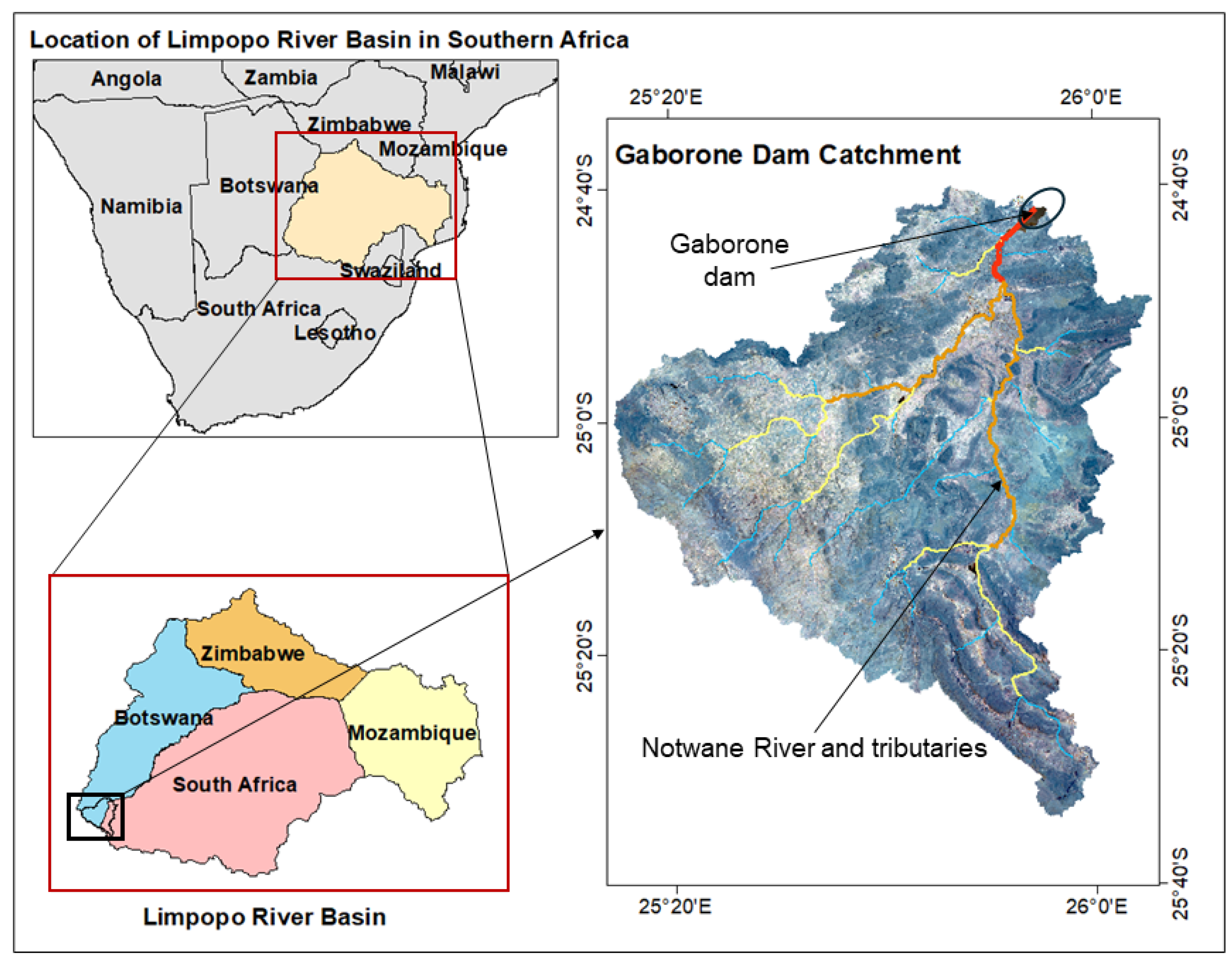
2.1. Study Area
2.2. Data
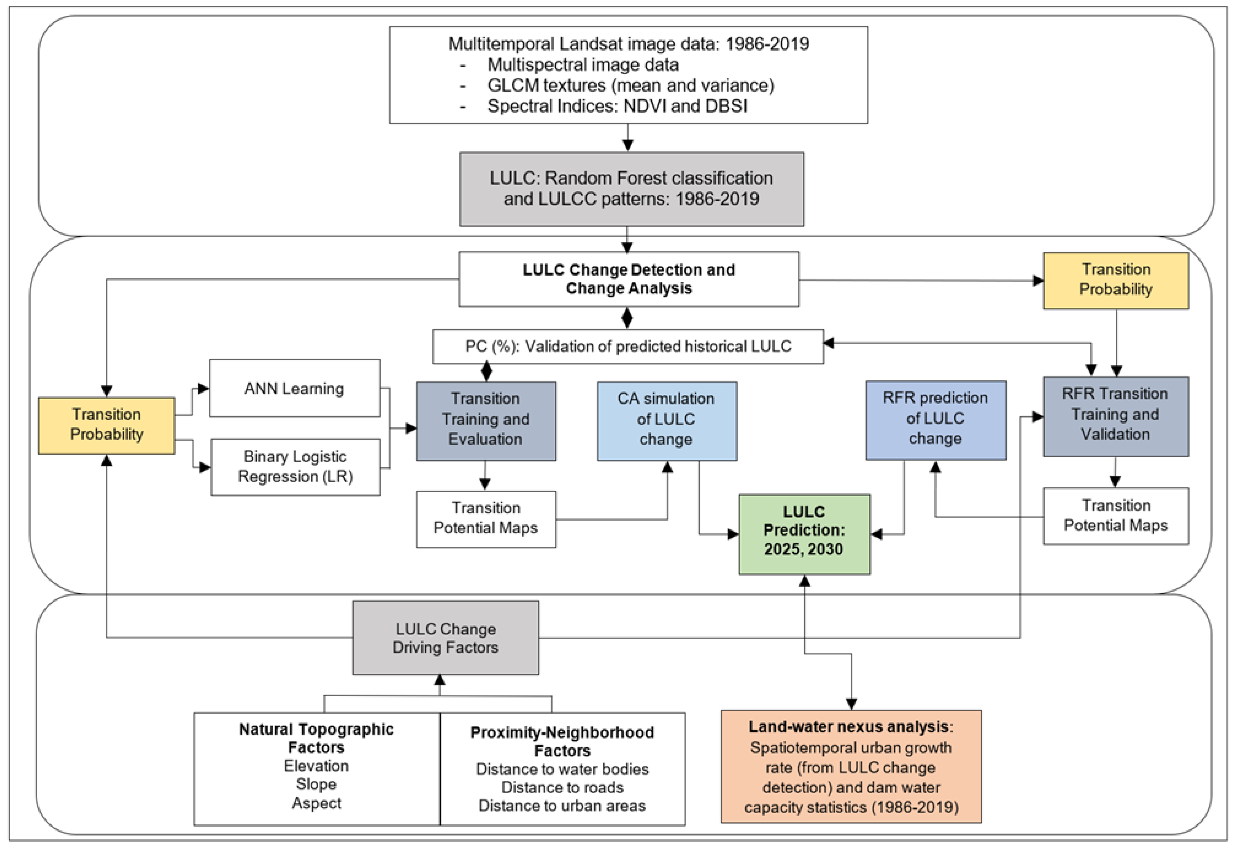
2.3. Methods
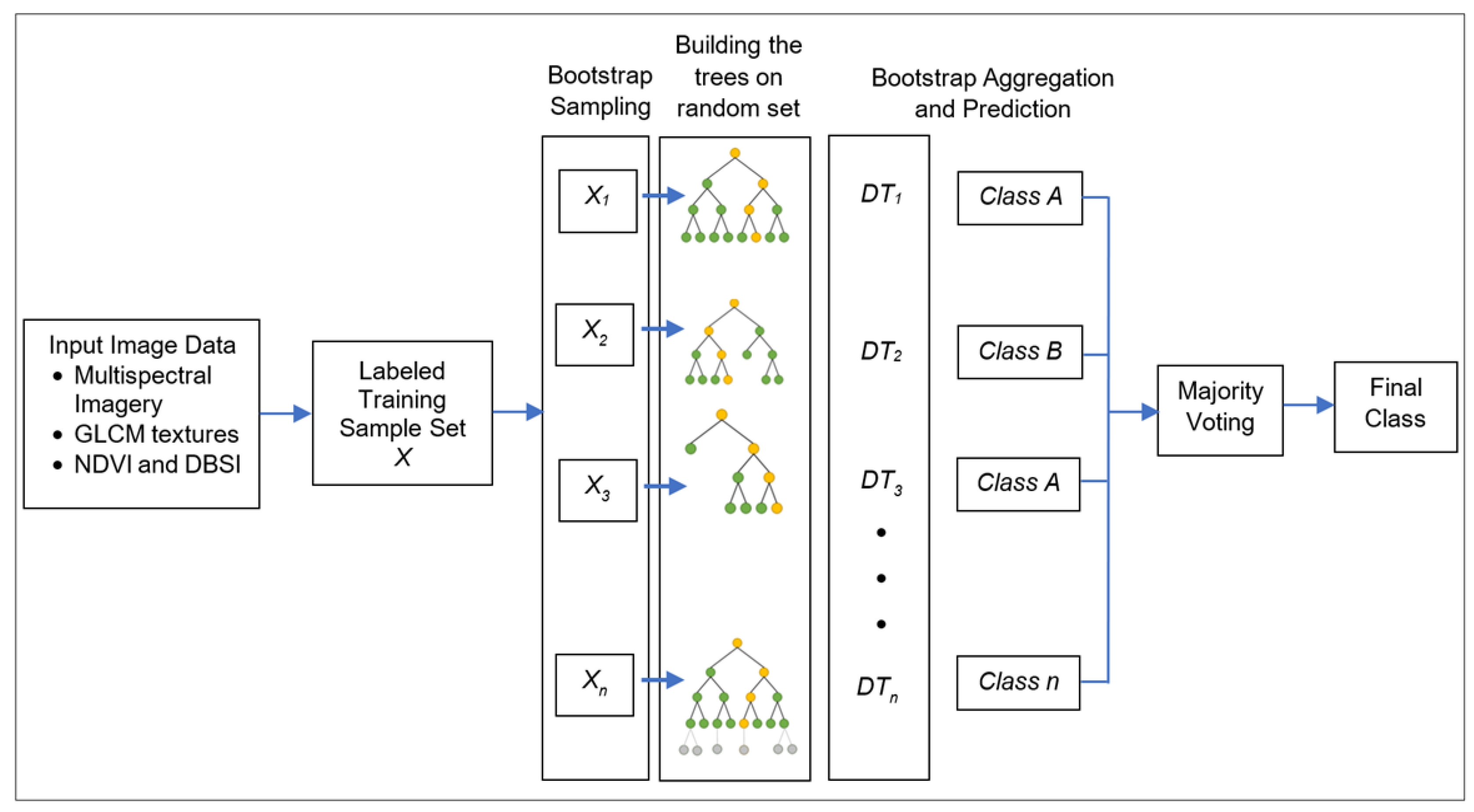
2.3.1. LULC Mapping Using Machine Learning with Multiple Input Features
2.3.2. Logistic Regression
2.3.3. Multilayer Perceptron (MLP) Artificial Neural Networks
2.3.4. Cellular Automata (CA) LULC Change Prediction Model
2.3.5. Random Forest Regression for LULC Prediction
2.3.6. Validation of LULC Prediction
3. Results
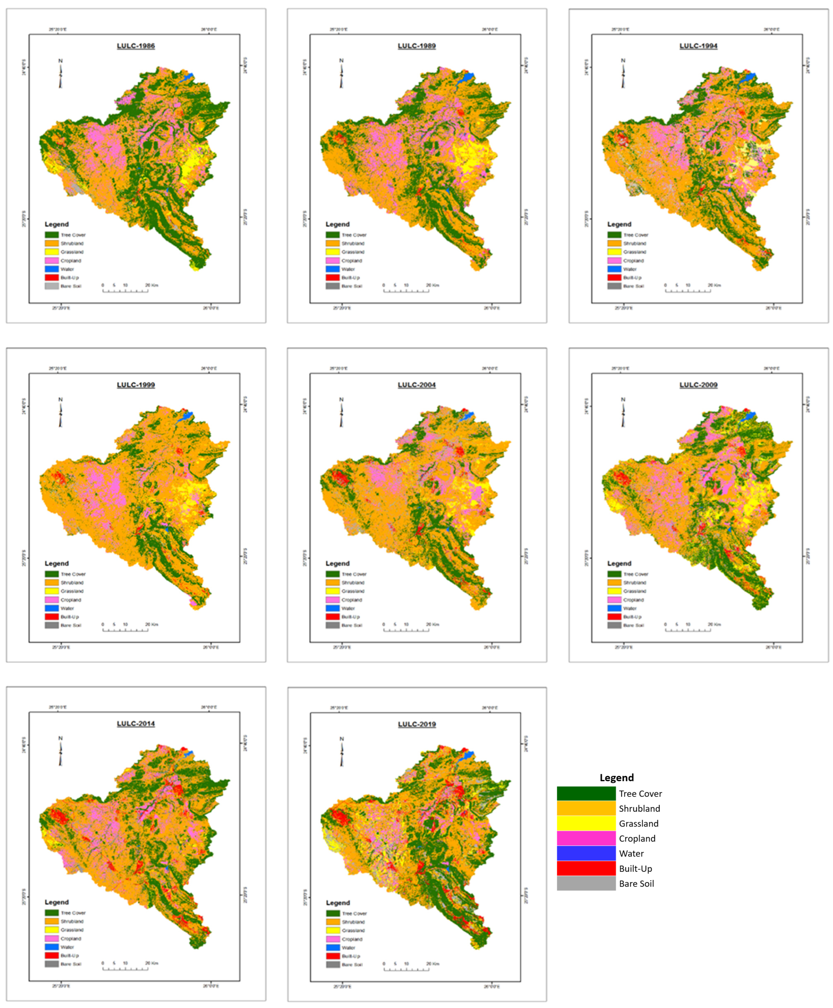
3.1. LULC Change Patterns in the Gaborone Dam Catchment
3.2. LULC Class Transition Analysis
3.3. Calibration of LULC Transition Potential
3.4. LULC Prediction for 2025 and 2030
4. Discussions
4.1. Comparison of the LULC Prediction Models
4.2. Case Study Assessment
4.3. Insights into LULC Change and Land–Water Sustainability
5. Conclusions
Author Contributions
Funding
Institutional Review Board Statement
Informed Consent Statement
Data Availability Statement
Conflicts of Interest
References
- Hoff, H.; Iceland, C.; Kuylenstierna, J.; Te Velde, D.W. Managing the water-land-energy nexus for sustainable development. UN Chron. 2012, 49, 4. [Google Scholar] [CrossRef]
- Abbas, Z.; Yang, G.; Zhong, Y.; Zhao, Y. Spatiotemporal change analysis and future scenario of LULC using the CA-ANN approach: A case study of the greater bay area, china. Land 2021, 10, 584. [Google Scholar] [CrossRef]
- Tirumala, R.D.; Tiwari, P. Importance of Land in SDG Policy Instruments: A Study of ASEAN Developing Countries. Land 2022, 11, 218. [Google Scholar] [CrossRef]
- Islam, K.; Rahman, M.F.; Jashimuddin, M. Modeling land use change using cellular automata and artificial neural network: The case of Chunati Wildlife Sanctuary, Bangladesh. Ecol. Indic. 2018, 88, 439–453. [Google Scholar] [CrossRef]
- Goldewijk, K.K. Estimating global land use change over the past 300 years: The HYDE database. Glob. Biogeochem. Cycles 2001, 15, 417–433. [Google Scholar] [CrossRef]
- Yirsaw, E.; Wu, W.; Shi, X.; Temesgen, H.; Bekele, B. Land use/land cover change modeling and the prediction of subsequent changes in ecosystem service values in a coastal area of China, the Su-Xi-Chang Region. Sustainability 2017, 9, 1204. [Google Scholar] [CrossRef]
- Abuelaish, B.; Olmedo, M.T.C. Scenario of land use and land cover change in the Gaza Strip using remote sensing and GIS models. Arab. J. Geosci. 2016, 9, 274. [Google Scholar] [CrossRef]
- Cao, M.; Chang, L.; Ma, S.; Zhao, Z.; Wu, K.; Hu, X.; Gu, Q.; Lü, G.; Chen, M. Multi-scenario simulation of land use for sustainable development goals. IEEE J. Sel. Top. Appl. Earth Obs. Remote Sens. 2022, 15, 2119–2127. [Google Scholar] [CrossRef]
- Duveiller, G.; Caporaso, L.; Abad-Viñas, R.; Perugini, L.; Grassi, G.; Arneth, A.; Cescatti, A. Local biophysical effects of land use and land cover change: Towards an assessment tool for policy makers. Land Use Policy 2020, 91, 104382. [Google Scholar] [CrossRef]
- Davin, E.L.; Rechid, D.; Breil, M.; Cardoso, R.M.; Coppola, E.; Hoffmann, P.; Jach, L.L.; Katragkou, E.; de Noblet-Ducoudré, N.; Radtke, K.; et al. Biogeophysical impacts of forestation in Europe: First results from the LUCAS (Land Use and Climate Across Scales) regional climate model intercomparison. Earth Syst. Dyn. 2020, 11, 183–200. [Google Scholar] [CrossRef]
- Cao, J.; Zhang, X.; Deo, R.; Gong, Y.; Feng, Q. Influence of stand type and stand age on soil carbon storage in China’s arid and semi-arid regions. Land Use Policy 2018, 78, 258–265. [Google Scholar] [CrossRef]
- Zhu, E.; Deng, J.; Zhou, M.; Gan, M.; Jiang, R.; Wang, K.; Shahtahmassebi, A. Carbon emissions induced by land-use and land-cover change from 1970 to 2010 in Zhejiang, China. Sci. Total Environ. 2019, 646, 930–939. [Google Scholar] [CrossRef] [PubMed]
- De Koning, G.H.J.; Benítez, P.C.; Muñoz, F.; Olschewski, R. Modelling the impacts of payments for biodiversity conservation on regional land-use patterns. Landsc. Urban Plan. 2007, 83, 255–267. [Google Scholar] [CrossRef]
- Xinyang, Y.; Qiang, Z.; Xiaomin, Y.; Sheng, W.; Xueyuan, R.; Funian, Z. An overview of distribution characteristics and formation mechanisms in global arid areas. Adv. Earth Sci. 2019, 34, 826. [Google Scholar]
- Meaza, H.; Tsegaye, D.; Nyssen, J. Allocation of degraded hillsides to landless farmers and improved livelihoods in Tigray, Ethiopia. Nor. Geogr. Tidsskr. Nor. J. Geogr. 2016, 70, 1–12. [Google Scholar] [CrossRef]
- Hoyer, R.; Chang, H. Assessment of freshwater ecosystem services in the Tualatin and Yamhill basins under climate change and urbanization. Appl. Geogr. 2014, 53, 402–416. [Google Scholar] [CrossRef]
- United Nations. The Sustainable Development Goals Report 2016; UN Department of Economic and Social Affairs: New York, NY, USA, 2016.
- Li, F.; Yigitcanlar, T.; Nepal, M.; Nguyen, K.; Dur, F. Machine Learning and Remote Sensing Integration for Leveraging Urban Sustainability: A Review and Framework. Sustain. Cities Soc. 2023, 96, 104653. [Google Scholar] [CrossRef]
- Milojevic-Dupont, N.; Creutzig, F. Machine learning for geographically differentiated climate change mitigation in urban areas. Sustain. Cities Soc. 2021, 64, 102526. [Google Scholar] [CrossRef]
- Mokhtari, Z.; Amani-Beni, M.; Asgarian, A.; Russo, A.; Qureshi, S.; Karami, A. Spatial prediction of the urban inter-annual land surface temperature variability: An integrated modeling approach in a rapidly urbanizing semi-arid region. Sustain. Cities Soc. 2023, 93, 104523. [Google Scholar] [CrossRef]
- Shorabeh, S.N.; Kakroodi, A.A.; Firozjaei, M.K.; Minaei, F.; Homaee, M. Impact assessment modeling of climatic conditions on spatial-temporal changes in surface biophysical properties driven by urban physical expansion using satellite images. Sustain. Cities Soc. 2022, 80, 103757. [Google Scholar] [CrossRef]
- Liping, C.; Yujun, S.; Saeed, S. Monitoring and predicting land use and land cover changes using remote sensing and GIS techniques—A case study of a hilly area, Jiangle, China. PLoS ONE 2018, 13, e0200493. [Google Scholar] [CrossRef]
- Wang, S.W.; Gebru, B.M.; Lamchin, M.; Kayastha, R.B.; Lee, W.K. Land use and land cover change detection and prediction in the Kathmandu district of Nepalusing remote sensing and GIS. Sustainability 2020, 12, 3925. [Google Scholar] [CrossRef]
- Hyandye, C.; Mandara, C.G.; Safari, J. GIS and logit regression model applications in land use/land cover change and distribution in Usangu catchment. Am. J. Remote Sens 2015, 3, 6–16. [Google Scholar] [CrossRef]
- Aitkenhead, M.J.; Aalders, I.H. Predicting land cover using GIS, Bayesian and evolutionary algorithm methods. J. Environ. Manag. 2009, 90, 236–250. [Google Scholar] [CrossRef]
- Lu, Y.; Wu, P.; Ma, X.; Li, X. Detection and prediction of land use/land cover change using spatiotemporal data fusion and the Cellular Automata–Markov model. Environ. Monit. Assess. 2019, 191, 68. [Google Scholar] [CrossRef]
- Yang, X.; Zheng, X.Q.; Lv, L.N. A spatiotemporal model of land use change based on ant colony optimization, Markov chain and cellular automata. Ecol. Model. 2012, 233, 11–19. [Google Scholar] [CrossRef]
- Subedi, P.; Subedi, K.; Thapa, B. Application of a hybrid cellularautomaton–Markov (CA-Markov) model in land-use change prediction: A case study of Saddle Creek Drainage Basin, Florida. Appl. Ecol. Environ. Sci. 2013, 1, 126–132. [Google Scholar]
- Stefanov, W.L.; Ramsey, M.S.; Christensen, P.R. Monitoring urban land cover change: An expert system approach to land cover classification of semiarid to arid urban centers. Remote Sens. Environ. 2001, 77, 173–185. [Google Scholar] [CrossRef]
- Ralha, C.G.; Abreu, C.G.; Coelho, C.G.; Zaghetto, A.; Macchiavello, B.; Machado, R.B. A multi-agent model system for land-use change simulation. Environ. Model. Softw. 2013, 42, 30–46. [Google Scholar] [CrossRef]
- Palmate, S.S.; Wagner, P.D.; Fohrer, N.; Pandey, A. Assessment of uncertainties in modelling land use change with an integrated cellular automata–Markov chain model. Environ. Model. Assess. 2022, 27, 275–293. [Google Scholar] [CrossRef]
- Jana, A.; Jat, M.K.; Saxena, A.; Choudhary, M. Prediction of land use land cover changes of a river basin using the CA-Markov model. Geocarto Int. 2022, 37, 14127–14147. [Google Scholar] [CrossRef]
- Sinha, P.; Kumar, L. Markov land cover change modeling using pairs oftime-series satellite images. Photogramm. Eng. Remote Sens. 2013, 79, 1037–1051. [Google Scholar] [CrossRef]
- Khan, A.M.; Li, Q.; Saqib, Z.; Khan, N.; Habib, T.; Khalid, N.; Majeed, M.; Tariq, A. MaxEnt modelling and impact of climate change on habitat suitability variations of economically important Chilgoza Pine (Pinus gerardiana Wall.) in South Asia. Forests 2022, 13, 715. [Google Scholar] [CrossRef]
- Saxena, A.; Jat, M.K.; Kumar, S. Sensitivity analysis and retrieval of optimum SLEUTH model parameters. Geocarto Int. 2022, 37, 7431–7444. [Google Scholar] [CrossRef]
- Puertas, O.L.; Henríquez, C.; Meza, F.J. Assessing spatial dynamics of urban growth using an integrated land use model. Application in Santiago Metropolitan Area, 2010–2045. Land Use Policy 2014, 38, 415–425. [Google Scholar]
- Han, H.; Yang, C.; Song, J. Scenario simulation and the prediction of land use and land cover change in Beijing, China. Sustainability 2015, 7, 4260–4279. [Google Scholar] [CrossRef]
- Keshtkar, H.; Voigt, W.; Alizadeh, E. Land-cover classification and analysis of change using machine-learning classifiers and multi-temporal remote sensing imagery. Arab. J. Geosci. 2017, 10, 154. [Google Scholar] [CrossRef]
- Rimal, B.; Zhang, L.; Keshtkar, H.; Haack, B.N.; Rijal, S.; Zhang, P. Land use/land cover dynamics and modeling of urban land expansion by the integration of cellular automata and markov chain. ISPRS Int. J. Geo-Inf. 2018, 7, 154. [Google Scholar] [CrossRef]
- Tariq, A.; Mumtaz, F.; Majeed, M.; Zeng, X. Spatio-temporalassessment of land use land cover based on trajectories and cellular automata Markov modelling and its impact on land surface temperature of Lahore district Pakistan. Environ. Monit. Assess. 2023, 195, 114. [Google Scholar] [CrossRef]
- Kocabas, V.; Dragicevic, S. Assessing cellular automata model behaviour using a sensitivity analysis approach. Comput. Environ. Urban Syst. 2006, 30, 921–953. [Google Scholar] [CrossRef]
- Ghosh, P.; Mukhopadhyay, A.; Chanda, A.; Mondal, P.; Akhand, A.; Mukherjee, S.; Nayak, S.K.; Ghosh, S.; Mitra, D.; Ghosh, T.; et al. Application of Cellular automata and Markov-chain model in geospatial environmental modeling-A review. Remote Sens. Appl. Soc. Environ. 2017, 5, 64–77. [Google Scholar] [CrossRef]
- Felegari, S.; Sharifi, A.; Moravej, K.; Golchin, A.; Tariq, A. Investigation of the relationship between ndvi index, soil moisture, and precipitation data using satellite images. Sustain. Agric. Syst. Technol. 2022, 314–325. [Google Scholar]
- Aburas, M.M.; Ho, Y.M.; Ramli, M.F.; Ash’aari, Z.H. Improving the capability of an integrated CA-Markov model to simulate spatio-temporal urban growth trends using an Analytical Hierarchy Process and Frequency Ratio. Int. J. Appl. Earth Obs. Geoinf. 2017, 59, 65–78. [Google Scholar] [CrossRef]
- Chaplot, V.; Le Brozec, E.C.; Silvera, N.; Valentin, C. Spatial and temporal assessment of linear erosion in catchments under sloping lands of northern Laos. Catena 2005, 63, 167–184. [Google Scholar] [CrossRef]
- Shahbazian, Z.; Faramarzi, M.; Rostami, N.; Mahdizadeh, H. Integrating logistic regression and cellular automata–Markov models with the experts’ perceptions for detecting and simulating land use changes and their driving forces. Environ. Monit. Assess. 2019, 191, 422. [Google Scholar] [CrossRef]
- Gu, G.; Wu, B.; Zhang, W.; Lu, R.; Feng, X.; Liao, W.; Pang, C.; Lu, S. Comparing machine learning methods for predicting land development intensity. PLoS ONE 2023, 18, e0282476. [Google Scholar] [CrossRef]
- Ozturk, D. Urban growth simulation of Atakum (Samsun, Turkey) using cellular automata-Markov chain and multi-layer perceptron-Markov chain models. Remote Sens. 2015, 7, 5918–5950. [Google Scholar] [CrossRef]
- Shafizadeh-Moghadam, H.; Asghari, A.; Tayyebi, A.; Taleai, M. Coupling machine learning, tree-based and statistical models with cellular automata to simulate urban growth. Comput. Environ. Urban Syst. 2017, 64, 297–308. [Google Scholar] [CrossRef]
- Arsanjani, J.J.; Helbich, M.; Kainz, W.; Boloorani, A.D. Integration of logistic regression, Markov chain and cellular automata models to simulate urban expansion. Int. J. Appl. Earth Obs. Geoinf. 2013, 21, 265–275. [Google Scholar] [CrossRef]
- Rienow, A.; Mustafa, A.; Krelaus, L.; Lindner, C. Modeling urban regions: Comparing random forest and support vector machines for cellular automata. Trans. GIS 2021, 25, 1625–1645. [Google Scholar] [CrossRef]
- Gounaridis, D.; Chorianopoulos, I.; Symeonakis, E.; Koukoulas, S. A Random Forest-Cellular Automata modelling approach to explore future land use/cover change in Attica (Greece), under different socio-economic realities and scales. Sci. Total Environ. 2019, 646, 320–335. [Google Scholar] [CrossRef]
- Zhang, X.; Zhou, J.; Song, W. Simulating urban sprawl in china based on the artificial neural network-cellular automata-Markov model. Sustainability 2020, 12, 4341. [Google Scholar] [CrossRef]
- Roy, B.; Rahman, M.Z. Spatio-temporal analysis and cellular automata-based simulations of biophysical indicators under the scenario of climate change and urbanization using artificial neural network. Remote Sens. Appl. Soc. Environ. 2023, 31, 100992. [Google Scholar] [CrossRef]
- Cuellar, Y.; Perez, L. Assessing the accuracy of sensitivity analysis: An application for a cellular automata model of Bogota’s urban wetland changes. Geocarto Int. 2023, 38, 2186491. [Google Scholar] [CrossRef]
- Zhang, X.; Ren, W.; Peng, H. Urban land use change simulation and spatial responses of ecosystem service value under multiple scenarios: A case study of Wuhan, China. Ecol. Indic. 2022, 144, 109526. [Google Scholar] [CrossRef]
- Ambarwulan, W.; Yulianto, F.; Widiatmaka, W.; Rahadiati, A.; Tarigan, S.D.; Firmansyah, I.; Hasibuan, M.A.S. Modelling land use/land cover projection using different scenarios in the Cisadane Watershed, Indonesia: Implication on deforestation and food security. Egypt. J. Remote Sens. Space Sci. 2023, 26, 273–283. [Google Scholar] [CrossRef]
- Pourmohammadi, P.; Adjeroh, D.A.; Strager, M.P.; Farid, Y.Z. Predicting developed land expansion using deep convolutional neural networks. Environ. Model. Softw. 2020, 134, 104751. [Google Scholar] [CrossRef]
- Fernald, A.; Tidwell, V.; Rivera, J.; Rodríguez, S.; Guldan, S.; Steele, C.; Ochoa, C.; Hurd, B.; Ortiz, M.; Koykin, K.; et al. Modeling sustainability of water, environment, livelihood, and culture in traditional irrigation communities and their linked watersheds. Sustainability 2012, 4, 2998–3022. [Google Scholar] [CrossRef]
- Hu, X.; Li, X.; Lu, L. Modeling the land use change in an arid oasis constrained by water resources and environmental policy change using cellular automata models. Sustainability 2018, 10, 2878. [Google Scholar] [CrossRef]
- Kamusoko, C.; Gamba, J. Simulating urban growth using a random forest-cellular automata (RF-CA) model. ISPRS Int. J. Geo-Inf. 2015, 4, 447–470. [Google Scholar] [CrossRef]
- Cetin, M.; Demirel, H. Modellingand simulation of urban dynamics. Fresenius Environ. Bull. 2010, 9, 2348–2353. [Google Scholar]
- Fu, X.; Wang, X.; Yang, Y.J. Deriving suitability factors for CA-Markov land use simulation model based on local historical data. J. Environ. Manag. 2018, 206, 10–19. [Google Scholar] [CrossRef] [PubMed]
- Berberoğlu, S.; Akın, A.; Clarke, K.C. Cellular automata modeling approaches to forecast urban growth for adana, Turkey: A comparative approach. Landsc. Urban Plan. 2016, 153, 11–27. [Google Scholar] [CrossRef]
- Pijanowski, B.C.; Tayyebi, A.; Doucette, J.; Pekin, B.K.; Braun, D.; Plourde, J. A big data urban growth simulation at a national scale: Configuring the GIS and neural network based land transformation model to run in a high performance computing (HPC) environment. Environ. Model. Softw. 2014, 51, 250–268. [Google Scholar] [CrossRef]
- Sajan, B.; Mishra, V.N.; Kanga, S.; Meraj, G.; Singh, S.K.; Kumar, P. Cellular automata-based artificial neural network model for assessing past, present, andfuture land use/land coverdynamics. Agronomy 2022, 12, 2772. [Google Scholar] [CrossRef]
- Saputra, M.H.; Lee, H.S. Prediction of land use and land cover changes for North Sumatra, Indonesia, using an artificial-neural-network-based cellular automaton. Sustainability 2019, 11, 3024. [Google Scholar] [CrossRef]
- Gharaibeh, A.; Shaamala, A.; Obeidat, R.; Al-Kofahi, S. Improving land-use change modeling by integrating ANN with Cellular Automata-Markov Chain model. Heliyon 2020, 6, e05092. [Google Scholar] [CrossRef]
- Ackerschott, A.; Kohlhase, E.; Vollmer, A.; Hörisch, J.; von Wehrden, H. Steering of land use in the context of sustainable development: A systematic review of economic instruments. Land Use Policy 2023, 129, 106620. [Google Scholar] [CrossRef]
- Ouma, Y.O.; Keitsile, A.; Nkwae, B.; Odirile, P.; Moalafhi, D.; Qi, J. Urban land-use classification using machine learning classifiers: Comparative evaluation and post-classification multi-feature fusion approach. Eur. J. Remote Sens. 2023, 56, 2173659. [Google Scholar] [CrossRef]
- Ouma, Y.; Nkwae, B.; Moalafhi, D.; Odirile, P.; Parida, B.; Anderson, G.; Qi, J. Comparison of machine learning classifiers for multitemporal and multisensor mapping of urban LULC features. Int. Arch. Photogramm. Remote Sens. Spat. Inf. Sci. 2022, 43, 681–689. [Google Scholar] [CrossRef]
- Biau, G.Ã.Š.; Scornet, E. A random forest guided tour. TEST 2016, 25, 197–227. [Google Scholar] [CrossRef]
- Li, X.; Yeh, A.G.O. Neural-network-based cellular automata for simulating multiple land use changes using GIS. Int. J. Geogr. Inf. Sci. 2002, 16, 323–343. [Google Scholar] [CrossRef]
- Jogun, T.; Lukić, A.; Gašparović, M. Simulation model of land cover changes in a post-socialist peripheral rural area: Požega-Slavonia County, Croatia. Croat. Geogr. Bull. 2019, 81, 31–59. [Google Scholar] [CrossRef]
- Santé, I.; García, A.M.; Miranda, D.; Crecente, R. Cellular automata models for the simulation of real-world urban processes: A review and analysis. Landsc. Urban Plan. 2010, 96, 108–122. [Google Scholar] [CrossRef]
- Memarian, H.; Balasundram, S.K.; Talib, J.B.; Sung, C.T.B.; Sood, A.M.; Abbaspour, K. Validation of CA-Markov for simulation of land use and cover change in the Langat Basin, Malaysia. J. Geogr. Inf. Syst. 2012, 4, 26322. [Google Scholar] [CrossRef]
- He, D.; Zhou, J.; Gao, W.; Guo, H.Y.U.S.; Yu, S.; Liu, Y. An integrated CA-markov model for dynamic simulation of land use change in Lake Dianchi watershed. Acta Sci. Nat. Univ. Pekin. 2014, 50, 1095–1105. [Google Scholar]
- Roodposhti, M.S.; Aryal, J.; Bryan, B.A. A novel algorithm for calculating transition potential in cellular automata models of land-use/cover change. Environ. Model. Softw. 2019, 112, 70–81. [Google Scholar] [CrossRef]
- Hewitt, R.; Díaz-Pacheco, J. Stable models for metastable systems? Lessons from sensitivity analysis of a cellular automata urban land use model. Comput. Environ. Urban Syst. 2017, 62, 113–124. [Google Scholar] [CrossRef]
- Wu, X.; Liu, X.; Zhang, D.; Zhang, J.; He, J.; Xu, X. Simulating mixed land-use change under multi-label concept by integrating a convolutional neural network and cellular automata: A case study of Huizhou, China. GIScience Remote Sens. 2022, 59, 609–632. [Google Scholar] [CrossRef]
- Roy, B. A machine learning approach to monitoring and forecasting spatio-temporal dynamics of land cover in Cox’s Bazar district, Bangladesh from 2001 to 2019. Environ. Chall. 2021, 5, 100237. [Google Scholar] [CrossRef]
- Gahegan, M. On the application of inductive machine learning tools to geographical analysis. Geogr. Anal. 2000, 32, 113–139. [Google Scholar] [CrossRef]
- Yan, W.; Meimei, X.; Yujia, T.; Huan, G.; Rong, C.; Zhiyi, S.; Xinying, A. Prediction and Early Warning Model for Environmental Data and Circulatory System Disease Death with Machine Learning. Data Anal. Knowl. Discov. 2022, 6, 79–92. [Google Scholar]
- Liu, J.; Shao, Q.; Yan, X.; Fan, J.; Zhan, J.; Deng, X.; Kuang, W.; Huang, L. The climatic impacts of land use and land cover change compared among countries. J. Geogr. Sci. 2016, 26, 889–903. [Google Scholar] [CrossRef]
- Tong, X.; Feng, Y. A review of assessment methods for cellular automata models of land-use change and urban growth. Int. J. Geogr. Inf. Sci. 2020, 34, 866–898. [Google Scholar] [CrossRef]
- Xu, Q.; Wang, Q.; Liu, J.; Liang, H. Simulation of land-use changes using the partitioned ANN-CA model and considering the influence of land-use change frequency. ISPRS Int. J. Geo-Inf. 2021, 10, 346. [Google Scholar] [CrossRef]
- Grinblat, Y.; Gilichinsky, M.; Benenson, I. Cellular automata modeling of land-use/land-cover dynamics: Questioning the reliability of data sources and classification methods. Ann. Am. Assoc. Geogr. 2016, 106, 1299–1320. [Google Scholar] [CrossRef]
- Guan, D.; Zhao, Z.; Tan, J. Dynamic simulation of land use change based onlogistic-CA-Markov and WLC-CA-Markov models: A case study in three gorges reservoir area of Chongqing, China. Environ. Sci. Pollut. Res. 2019, 26, 20669–20688. [Google Scholar] [CrossRef] [PubMed]
- Siddiqui, A.; Siddiqui, A.; Maithani, S.; Jha, A.K.; Kumar, P.; Srivastav, S.K. Urban growth dynamics of an Indian metropolitan using CA Markov and Logistic Regression. Egypt. J. Remote Sens. Space Sci. 2018, 21, 229–236. [Google Scholar] [CrossRef]
- He, J.; Li, X.; Yao, Y.; Hong, Y.; Jinbao, Z. Mining transition rules of cellular automata for simulating urban expansion by using the deep learning techniques. Int. J. Geogr. Inf. Sci. 2018, 32, 2076–2097. [Google Scholar] [CrossRef]
- Saadani, S.; Laajaj, R.; Maanan, M.; Rhinane, H.; Aaroud, A. Simulating spatial–temporalurban growth of a Moroccan metropolitan using CA–Markov model. Spat. Inf. Res. 2020, 28, 609–621. [Google Scholar] [CrossRef]
- Liu, Y.; Cao, X.; Li, T. Identifying driving forces of built-up land expansion based on the geographical detector: A case study of Pearl River Delta urban agglomeration. Int. J. Environ. Res. Public Health 2020, 17, 1759. [Google Scholar] [CrossRef] [PubMed]
- Mozaffaree Pour, N.; Oja, T. Prediction power of logistic regression (LR) and Multi-Layer perceptron (MLP) models in exploring driving forces of urban expansion to be sustainable in estonia. Sustainability 2021, 14, 160. [Google Scholar] [CrossRef]
- Ullah, S.; Ahmad, K.; Sajjad, R.U.; Abbasi, A.M.; Nazeer, A.; Tahir, A.A. Analysis and simulation of land cover changes and their impacts on land surface temperature inalower Himalayan region. J. Environ. Manag. 2019, 245, 348–357. [Google Scholar] [CrossRef] [PubMed]
- Saha, T.K.; Pal, S.; Sarkar, R. Prediction of wetland area and depth using linear regression model and artificial neural network based cellular automata. Ecol. Inform. 2021, 62, 101272. [Google Scholar] [CrossRef]
- Mohamed, A.; Worku, H. Simulating urban land use and cover dynamics using cellular automata and Markov chain approach in Addis Ababa and the surrounding. Urban Clim. 2020, 31, 100545. [Google Scholar] [CrossRef]
- Cannemi, M.; García-Melón, M.; Aragonés-Beltrán, P.; Gómez-Navarro, T. Modeling decision making as a support tool for policy making on renewable energy development. Energy Policy 2014, 67, 127–137. [Google Scholar] [CrossRef]
- Girma, R.; Fürst, C.; Moges, A. Land use land cover change modeling by integrating artificial neural network with cellular Automata-Markov chain model in Gidabo river basin, main Ethiopian rift. Environ. Chall. 2022, 6, 100419. [Google Scholar] [CrossRef]
- Singh, S.K.; Mustak, S.; Srivastava, P.K.; Szabó, S.; Islam, T. Predicting spatial and decadal LULC changes through cellular automata Markov chain models using earth observation datasets and geo-information. Environ. Process. 2015, 2, 61–78. [Google Scholar] [CrossRef]
- Maithani, S. A neural network based urban growth model of an Indian city. J. Indian Soc. Remote Sens. 2009, 37, 363–376. [Google Scholar] [CrossRef]
- Zhou, Y.; Zhang, F.; Du, Z.; Ye, X.; Liu, R. Integrating cellular automata with the deep belief network for simulating urban growth. Sustainability 2017, 9, 1786. [Google Scholar] [CrossRef]
- Simwanda, M.; Murayama, Y.; Ranagalage, M. Modeling the drivers of urban land use changes in Lusaka, Zambia using multi-criteria evaluation: An analytic network process approach. Land Use Policy 2020, 92, 104441. [Google Scholar] [CrossRef]
- Karimi, F.; Sultana, S.; Babakan, A.S.; Suthaharan, S. An enhanced support vector machine model for urban expansion prediction. Comput. Environ. Urban Syst. 2019, 75, 61–75. [Google Scholar] [CrossRef]
- Msofe, N.K.; Sheng, L.; Lyimo, J. Land use change trends and theirdriving forces in the Kilombero Valley Floodplain, Southeastern Tanzania. Sustainability 2019, 11, 505. [Google Scholar] [CrossRef]
- Bonilla-Bedoya, S.; Mora, A.; Vaca, A.; Estrella, A.; Herrera, M.Á. Modelling the relationship between urban expansion processes and urban forest characteristics: An application to the Metropolitan District of Quito. Comput. Environ. Urban Syst. 2020, 79, 101420. [Google Scholar] [CrossRef]
- Rahnama, M.R. Forecasting land-use changes in Mashhad Metropolitan area usingCellular Automata and Markovchain model for 2016–2030. Sustain. Cities Soc. 2021, 64, 102548. [Google Scholar] [CrossRef]
- Turner, B.L.; Lambin, E.F.; Reenberg, A. The emergence of land change science for global environmental change and sustainability. Proc. Natl. Acad. Sci. USA 2007, 104, 0666–20671. [Google Scholar] [CrossRef] [PubMed]
- Shukla, S.; Meshesha, T.W.; Sen, I.S.; Bol, R.; Bogena, H.; Wang, J. Assessing Impacts of Land Use and Land Cover (LULC) Change on Stream Flow and Runoff in Rur Basin, Germany. Sustainability 2023, 15, 9811. [Google Scholar] [CrossRef]
- UN-Water. Water and Climate Change. The United Nations World Water Development Report; UNESCO: Paris, France, 2020. [Google Scholar]
- Kong, X.; Fu, M.; Zhao, X.; Wang, J.; Jiang, P. Ecological effects of land-use change on two sides of the Hu Huanyong Line in China. Land Use Policy 2022, 113, 105895. [Google Scholar] [CrossRef]
- Lafuite, A.-S.; Denise, G.; Loreau, M. Sustainable land-use management under biodiversity lag effects. Ecol. Econ. 2018, 154, 272–281. [Google Scholar] [CrossRef]
- Welde, K.; Gebremariam, B. Effect of land use land cover dynamics on hydrological response of watershed: Case study of Tekeze Dam watershed, northern Ethiopia. Int. Soil Water Conserv. Res. 2017, 5, 1–16. [Google Scholar] [CrossRef]
- Murmu, P.; Kumar, M.; Lal, D.; Sonker, I.; Singh, S.K. Delineation of groundwater potential zones using geospatial techniquesandanalytical hierarchy processin Dumka district, Jharkhand, India. Groundw. Sustain. Dev. 2019, 9, 100239. [Google Scholar] [CrossRef]
- Zachrisson, A.; Bjärstig, T.; Thellbro, C.; Neumann, W.; Svensson, J. Participatory comprehensive planning to handle competing land-use priorities in the sparsely populated rural context. J. Rural Stud. 2021, 88, 1–13. [Google Scholar] [CrossRef]
- Loveland, T.R.; Mahmood, R. A design for a sustained assessment of climate forcing and feedbacks related to land use and land cover change. Bull. Am. Meteorol. Soc. 2014, 95, 1563–1572. [Google Scholar] [CrossRef]
- Scanlon, B.R.; Reedy, R.C.; Stonestrom, D.A.; Prudic, D.E.; Dennehy, K.F. Impact of land use and land cover change on groundwater recharge and quality in the southwestern US. Glob. Change Biol. 2005, 11, 1577–1593. [Google Scholar] [CrossRef]
- Pauliuk, S.; Heeren, N. Material efficiency and its contribution to climate change mitigation in Germany: A deep decarbonization scenario analysis until 2060. J. Ind. Ecol. 2021, 25, 479–493. [Google Scholar] [CrossRef]


| Factor Category | Data | Data Sources/Spatial Resolution | Data Description | Units |
|---|---|---|---|---|
| Natural topographic factors | Elevation | ALOS-PALSAR DEM https://search.asf.alaska.edu/#/ (accesssed on 24 November 2022) 12.5 m × 12.5 m | DEM | m |
| Slope | Range from 0 to 90 | Degrees (°) | ||
| Aspect | Range from 0 to 360 | Degrees (°) | ||
| Proximity-neighborhood factors | Distance to water bodies | Euclidean distance to water bodies | km | |
| Distance to roads | Digitized from Google Earth image https://earth.google.com/web/ (accessed on 12 July 2023) | Euclidean distance to roads and railway lines | km | |
| Distance to urban areas | Euclidean distance to significant residential points | km | ||
| Land use and land cover | Land use land cover (LULC) from Landsat TM and ETM+ | Landsat data https://earthexplorer.usgs.gov/ (accessed on 24 November 2022) 30 m × 30 m | Land use land cover for respective years | km2; % |
| Year | 1986 | 1989 | 1994 | 1999 | 2004 | 2009 | 2014 | 2019 |
|---|---|---|---|---|---|---|---|---|
| OA (%) | 88.9 | 89.1 | 83.4 | 85.2 | 89.6 | 81.3 | 85.2 | 84.8 |
| Kappa Index | 0.82 | 0.84 | 0.76 | 0.78 | 0.84 | 0.74 | 0.78 | 0.80 |
| Class | Transition Years | Tree Cover | Shrub/ Grassland | Cropland | Water | Built-Up | Bare Soil |
|---|---|---|---|---|---|---|---|
| Tree Cover | 1986–1989 | 0.5778 | 0.3707 | 0.0337 | 0.0001 | 0.0050 | 0.0128 |
| 1989–1994 | 0.6325 | 0.3181 | 0.0321 | 0.0004 | 0.0051 | 0.0119 | |
| 1994–1999 | 0.4730 | 0.5014 | 0.0152 | 0.0005 | 0.0038 | 0.0060 | |
| 1999–2004 | 0.6582 | 0.2967 | 0.0275 | 0.0005 | 0.0036 | 0.0135 | |
| 2004–2009 | 0.6393 | 0.3118 | 0.0283 | 0.0007 | 0.0089 | 0.0110 | |
| 2009–2014 | 0.6140 | 0.3443 | 0.0190 | 0.0000 | 0.0102 | 0.0125 | |
| 2014–2019 | 0.7236 | 0.2295 | 0.0096 | 0.0003 | 0.0034 | 0.0337 | |
| Shrub/ Grassland | 1986–1989 | 0.0923 | 0.7340 | 0.1253 | 0.0047 | 0.0116 | 0.0321 |
| 1989–1994 | 0.1380 | 0.7087 | 0.1028 | 0.0001 | 0.0086 | 0.0418 | |
| 1994–1999 | 0.0827 | 0.8294 | 0.0681 | 0.0000 | 0.0111 | 0.0086 | |
| 1999–2004 | 0.1192 | 0.7185 | 0.0944 | 0.0001 | 0.0192 | 0.0486 | |
| 2004–2009 | 0.2101 | 0.6390 | 0.1113 | 0.0002 | 0.0119 | 0.0275 | |
| 2009–2014 | 0.1978 | 0.6534 | 0.0980 | 0.0000 | 0.0235 | 0.0272 | |
| 2014–2019 | 0.1974 | 0.6336 | 0.0463 | 0.0017 | 0.0209 | 0.1001 | |
| Cropland | 1986–1989 | 0.0322 | 0.3578 | 0.5700 | 0.0000 | 0.0039 | 0.0361 |
| 1989–1994 | 0.0301 | 0.4002 | 0.4400 | 0.0001 | 0.0081 | 0.1215 | |
| 1994–1999 | 0.0411 | 0.5430 | 0.3732 | 0.0003 | 0.0204 | 0.0220 | |
| 1999–2004 | 0.0243 | 0.5294 | 0.3115 | 0.0002 | 0.0151 | 0.1194 | |
| 2004–2009 | 0.0545 | 0.4629 | 0.4363 | 0.0001 | 0.0092 | 0.0369 | |
| 2009–2014 | 0.0458 | 0.4496 | 0.4253 | 0.0000 | 0.0266 | 0.0527 | |
| 2014–2019 | 0.0515 | 0.5369 | 0.2693 | 0.0005 | 0.0165 | 0.1253 | |
| Water | 1986–1989 | 0.0691 | 0.0208 | 0.0048 | 0.8798 | 0.0063 | 0.0192 |
| 1989–1994 | 0.1453 | 0.0173 | 0.0300 | 0.7524 | 0.0264 | 0.0287 | |
| 1994–1999 | 0.0275 | 0.0248 | 0.0071 | 0.8268 | 0.0212 | 0.0926 | |
| 1999–2004 | 0.0139 | 0.0122 | 0.0012 | 0.7526 | 0.0010 | 0.2191 | |
| 2004–2009 | 0.0012 | 0.0088 | 0.0000 | 0.9666 | 0.0003 | 0.0230 | |
| 2009–2014 | 0.0355 | 0.2053 | 0.0162 | 0.3918 | 0.0035 | 0.3478 | |
| 2014–2019 | 0.0216 | 0.0024 | 0.0000 | 0.9317 | 0.0098 | 0.0346 | |
| Built-Up | 1986–1989 | 0.1020 | 0.5229 | 0.0652 | 0.0004 | 0.2097 | 0.0999 |
| 1989–1994 | 0.0666 | 0.3962 | 0.0712 | 0.0005 | 0.3788 | 0.0867 | |
| 1994–1999 | 0.0242 | 0.5414 | 0.0418 | 0.0010 | 0.3441 | 0.0475 | |
| 1999–2004 | 0.0661 | 0.3315 | 0.0793 | 0.0024 | 0.3893 | 0.1315 | |
| 2004–2009 | 0.0496 | 0.3207 | 0.0460 | 0.0005 | 0.4885 | 0.0947 | |
| 2009–2014 | 0.0322 | 0.2954 | 0.0375 | 0.0001 | 0.6021 | 0.0327 | |
| 2014–2019 | 0.0634 | 0.2100 | 0.0145 | 0.0002 | 0.6237 | 0.0882 | |
| Bare Soil | 1986–1989 | 0.0870 | 0.6300 | 0.1738 | 0.0009 | 0.0128 | 0.0955 |
| 1989–1994 | 0.0844 | 0.5060 | 0.1777 | 0.0023 | 0.0599 | 0.1698 | |
| 1994–1999 | 0.0253 | 0.4538 | 0.3042 | 0.0005 | 0.0377 | 0.1785 | |
| 1999–2004 | 0.0759 | 0.3237 | 0.1213 | 0.0033 | 0.0528 | 0.4230 | |
| 2004–2009 | 0.0638 | 0.3489 | 0.2565 | 0.0196 | 0.0675 | 0.2437 | |
| 2009–2014 | 0.0258 | 0.4204 | 0.1446 | 0.0016 | 0.1195 | 0.2882 | |
| 2014–2019 | 0.0496 | 0.4067 | 0.0463 | 0.0375 | 0.0485 | 0.4115 |
| 5-Year LULC Predictions (%) | ||||||
|---|---|---|---|---|---|---|
| LULC Class | LR-CA | ANN-CA | RFR | |||
| 2019–2025 | 2025–2030 | 2019–2025 | 2025–2030 | 2019–2025 | 2025–2030 | |
| Tree Cover | −0.01 | 0.00 | −0.02 | 0.00 | −0.55 | −0.12 |
| Shrubland/Grassland | 0.04 | −0.01 | −0.02 | −0.17 | 0.34 | −9.25 |
| Cropland | −0.59 | −0.17 | −0.60 | −0.17 | 0.07 | −2.91 |
| Water | −0.01 | 0.00 | −0.01 | 0.00 | 0.01 | 0.04 |
| Built-Up | 0.08 | 0.07 | 0.07 | 0.07 | 0.95 | 1.63 |
| Bare Soil | 0.48 | 0.11 | 0.47 | 0.12 | 0.14 | 8.65 |
Disclaimer/Publisher’s Note: The statements, opinions and data contained in all publications are solely those of the individual author(s) and contributor(s) and not of MDPI and/or the editor(s). MDPI and/or the editor(s) disclaim responsibility for any injury to people or property resulting from any ideas, methods, instructions or products referred to in the content. |
© 2024 by the authors. Licensee MDPI, Basel, Switzerland. This article is an open access article distributed under the terms and conditions of the Creative Commons Attribution (CC BY) license (https://creativecommons.org/licenses/by/4.0/).
Share and Cite
Ouma, Y.O.; Nkwae, B.; Odirile, P.; Moalafhi, D.B.; Anderson, G.; Parida, B.; Qi, J. Land-Use Change Prediction in Dam Catchment Using Logistic Regression-CA, ANN-CA and Random Forest Regression and Implications for Sustainable Land–Water Nexus. Sustainability 2024, 16, 1699. https://doi.org/10.3390/su16041699
Ouma YO, Nkwae B, Odirile P, Moalafhi DB, Anderson G, Parida B, Qi J. Land-Use Change Prediction in Dam Catchment Using Logistic Regression-CA, ANN-CA and Random Forest Regression and Implications for Sustainable Land–Water Nexus. Sustainability. 2024; 16(4):1699. https://doi.org/10.3390/su16041699
Chicago/Turabian StyleOuma, Yashon O., Boipuso Nkwae, Phillimon Odirile, Ditiro B. Moalafhi, George Anderson, Bhagabat Parida, and Jiaguo Qi. 2024. "Land-Use Change Prediction in Dam Catchment Using Logistic Regression-CA, ANN-CA and Random Forest Regression and Implications for Sustainable Land–Water Nexus" Sustainability 16, no. 4: 1699. https://doi.org/10.3390/su16041699
APA StyleOuma, Y. O., Nkwae, B., Odirile, P., Moalafhi, D. B., Anderson, G., Parida, B., & Qi, J. (2024). Land-Use Change Prediction in Dam Catchment Using Logistic Regression-CA, ANN-CA and Random Forest Regression and Implications for Sustainable Land–Water Nexus. Sustainability, 16(4), 1699. https://doi.org/10.3390/su16041699