A System Dynamics Approach to Valorize Overripe Figs in the Brewing of Artisanal Beer

Abstract

Craft beer production has grown extensively worldwide. The variety of products and grains that can be used in production make this artisanal product unique. In this study, we propose a system dynamics model that allows for the evaluation of different production scenarios in which figs are used as the main ingredient. This research is inspired by the real case of small fig producers in Valle del Mayo in Navojoa, Sonora, Mexico, who, in 2020, took on the challenge of creating a processing factory for fig-derived products. This paper presents the development and application of a system dynamics approach to model the entire supply chain of overripe figs, i.e., figs that cannot be marketed in prime quality but can still be used in the production of derivative products. The method used for its development encompasses the following stages: (1) defining the craft beer supply chain variables; (2) elaborating on causal diagrams; (3) producing model stock and flow diagrams; (4) model validation; (5) sensitivity analysis and scenario evaluations; and (6) building a graphical user interface (GUI). The proposed model allows managers to assess several production policies under various assumptions of capacity and beer demand, demonstrating its value as an effective tool for strategic decision making.

1. Introduction

The first references to beer consumption originate from Mesopotamia in the year 7000 B.C. In the present day, different types of industrial beer are manufactured by prominent corporations with the use of very efficient industrial processes and under high standards of production and flavors, as identified by consumers [1]. However, in more recent years, the number of craft breweries has increased rapidly, and the fundamental aim of producers is to offer a product with a different experience in terms of flavor and aroma besides simply offering beer of high quality.

In 2023, the Mexican brewery association ACEMEX (Asociación Cervecera de la República Mexicana) proposed a labeling system that establishes three categories for beer producers in Mexico: Independientes, Artesanales, and Mexicanas [1]. First, Mexicanas refers to any beer produced in the country. Second, Independientes (independent) refers to beer from producers that are not owned, or are participated in by more than 25%, by one of the large industrial companies that dominates the Mexican market. Finally, Artesanales, or craft, refers to beer produced by small breweries with production under 1% of the total beer produced in the country. Craft producers can be distinguished by the excellence of their brewing processes and the quality of ingredients used, including 100% malt and low additives only, which are used for developing recipes for innovative creations with the purpose of enhancing flavors and not just for reducing production costs. This research project was developed in partnership with a craft producer in Valle del Mayo, Navojoa, Sonora, Mexico, who, in 2022, desired to introduce figs as one of the raw ingredients in the production of craft beer [2].

The fig is a perishable product, so it requires care and attention to ensure freshness. Figs need to be kept cold to maintain their nutritional properties and, more importantly, their shelf life, which is one of the major challenges in the supply chain before they are sold on local or international markets. For example, our partners recognize that, on average, for each ton harvested, only half a ton reaches the final market in one week (the estimated shelf life of figs); the rest loses its quality and, in particular, its freshness because the producers do not own cold rooms to preserve the product. Cold rooms are indeed expensive and require high investments that can only be justified by large volumes of figs. An alternative business option based on the valorization of overripe figs was suggested. The idea was to use figs that are not as fresh as an ingredient in the production of craft beer so that the economic losses could be compensated or at least minimized by the income derived from the sale of overripe figs.

A pilot was conducted to elaborate on this new beer brewing process and to estimate its productivity. Essentially, the idea was to replace part of the fermentable sugar produced by starch in the cereal with the ones in the figs. However, when doing so, one must be careful to account for fig fermentable sugar when developing the malt bill. In addition, figs darken the color of the liquid and lend “body” to the beer. Furthermore, a decision needs to be made concerning when to add figs to the production process (i.e., during boiling or during secondary fermentation). Therefore, establishing the appropriate recipe involved a lengthy empirical process that included several tests and trials. Even now, the basic recipe needs to be slightly modified from batch to batch in order to adapt the product to the variability of the raw ingredients. In this base recipe, 3 kg of figs yields 18 L of beer. The initial goal of our partners was to produce 250 bottles of beer per month (with each bottle containing 0.5 L of beer) and the expected sales price was set to MXN 50 per bottle.

In this context, in the early stages of their initiative, our partners identified the need for decision-making tools able to support them in assessing the feasibility of their goals, defining commercial strategies, and helping in the elaboration of effective production plans. This paper reports our research on the design and implementation of a system dynamics model with a graphical user interface able to capture the whole overripe figs supply chain as part of a sustainable approach and to evaluate its performance under different scenarios. As the main input, we use the number of harvested figs per season that cannot be placed on the market for consumption due to the deterioration in specific properties, mainly freshness. With this, overripe figs are utilized in the craft beer production process.

2. Materials and Methods

To meet our partners’ needs, we decided to develop a decision support tool encompassing a system dynamics model that might accurately represent craft beer production and allow us to estimate its performance under different scenarios defined by the managers. System dynamics methodology incorporates variables and parameters, which are simulated in complex environments that represent current and future policies, in a time horizon determined by decision makers [3]. For this purpose, processing maps and causal models were built based on systemic thinking [4,5,6].

Causal diagrams allow for the analysis of the cause–effect relationship between the variables and the parameters that conform to the system dynamics model with two distinct behaviors named balance (B) and reinforcement (R). These dynamics jointly allow for modeling of the different interconnected loops in order to understand the complexity and relationships of the contemplated stages [7]. Thus, the different models may be constructed as proposed by Kania et al. [8], with them allowing for simple implementation using specialized software. Additionally, conclusions are generated from the data, supporting decision making with quantitative information [9,10]. In the same manner, Ford [11] emphasized the importance of building loops to adequately capture the behavior of systems and the need for automated tools able to simulate or solve numerical models encompassing multiple loops.

For craft beer system dynamics model simulation, Stella^® Architect 2023 (Versión 3.3, Isee Systems Inc., Lebanon, NH, USA) was used. This simulator uses an algorithm for solving differential equations with Runge Kutta or Euler numeric methods [12] based on the proposals of Chapra et al. [13] and Negar et al. [14]. Subsequently, validation of the model was carried out following the method proposed by Kleijnen [15] and Barlas and Carpenter [16].

In the next stage, a sensitivity analysis was performed to evaluate the different scenarios in pessimistic and optimistic situations starting from the current scenario given by the model response initially executed [17]. To select the scenarios, two techniques were used: (1) the technique for order of preference by similarity (TOPSIS), a multicriteria method whose aim is to rank in order of choice a certain number of alternatives based on a set of favorable or unfavorable criteria [18,19,20]; and (2) Faire Un Choix Adéquat (FUCA), which is based on a linear combination of the ranks that each alternative obtains with respect to each individual criterion [21].

Finally, we integrated the solution for the producers into a series of visual elements that help with and allow for interaction with the system in the most simple and user-friendly manner; buttons and graphical elements were used for their understanding and were supported by the graphical user interface [22,23,24].

To sum up, the method proposed in the previous paragraphs can be formalized into the following six steps:

• Determining the variables that compose the causal model. The variables related to the fig supply chain, the production process, and craft beer sales, as well as the parameters, were identified and classified.
• Designing the causal diagram. We connected the variables and parameters with feedback loops (reinforcement (R) and balance (B)) to reproduce the causal behavior of the craft beer supply chain. Causal models were elaborated with Vensim^® PLE Plus (Version 9.4.2, Ventana System Inc., Harvard, MA, USA, 2019).
• Developing the stock and flow diagram with mathematical equations. For the construction of the level and flow diagram, Stella^® Architect 2023 (Version 3.3, Isee Systems Inc., Lebanon, NH, USA) was used. Based on the causal diagrams, a set of differential equations was proposed to represent the dynamic relationships between the variables and parameters defined in the previous stages.
• Validating the model using the current scenario. Simulation runs were performed using the current craft beer manufacturing conditions. The simulation outcomes were compared to the actual process to assess the model’s ability to reproduce the real manufacturing dynamics.
• Simulating the current, optimistic, and pessimistic scenarios. Two multicriteria analysis methods (FUCA and TOPSIS) were used to select the best options produced for the pessimistic, optimistic, and current operations scenarios.
• Development of a graphical user interface. This represents the last step in the technological solution (graphical user interface). The goal was to allow the user to incorporate new data into the model and run simulations for decision-making purposes.

The next section explains how each of the proposed steps was implemented and presents the results they produced.

3. Results and Discussion

3.1. Defining the Craft Beer Supply Chain Variables

To identify and select the variables and parameters of the model, we carried out interviews with experts from the brewery. With their help, we modeled the most important stages of the craft beer production process and carried out observations at the production plant. These final sets of variables and parameters, reported in

Table 1. List of IDs, variables, and definitions of craft beer production.

Id	Variable	Definition
2	Fig inventory for beer	Number of figs stored for craft beer production (kg)
1	Inflow of figs	Daily number of figs arriving to the system (kg/day)
3	Fig inventory discrepancy	Difference between the capacity of the fig warehouse inventory and the fig inventory for craft beer physically in the warehouse (kg)
22	Fig input to fermentation	Fig quantity passing to the fermenting mixture (kg/day)
I	Resting time	Resting time in fermentation (days)
b	Storage capacity for figs	Maximum number of figs that can be stored at the warehouse (kg)
a	Time to fill fig orders	Average time used for order delivery to the craft beer factory (kg/day)
14	Malt mashing	Amount of mixed grain and water needed to activate enzymes and extract sugars (L)
16	Wort–yeast inflow	Daily inflow of wort–yeast (L/day)
17	Outflow fermentation	Daily outflow of the fermentation process (L/day)
16	Wort and yeast inventory	Wort–yeast inventory (L)
h	% of yeast fermentation	Daily percentage of wort and yeast in the fermentation (80% to 100%/day)
4	Fermented beer	Inventory of fermented beer (L)
18	Inflow to rest	Fermentation process inflow (L/day)
g	% Inventory required	Inventory percentage required for the outflow fermentation process (%/day)
19	Resting–fermentation	Seven-day fermentation process (L/day)
20	Outflow of craft beer	Daily craft beer outflow (L)
5	Inventory of beer in the depot	Craft beer in storage deposits (L)
21	Bottling	Daily craft beer liters passing to the bottling process (L/day)
6	Flow to beer warehouse	Craft beer inflow quantity to the bottling process (bottles/day)
f	Liter conversion to bottles	Craft beer liter conversion to half-liter bottles (bottles/day)
7	Beer inventory	Number of craft beer bottles in the warehouse (bottles)
9	Discrepancy in inventory	Bottle inventory discrepancy versus warehouse capacity (bottles)
d	Craft beer cellar capacity	Craft beer cellar capacity for storage (bottles)
8	Craft beer sales	Craft beer sales per day (bottles/day)
10	Revenue	Income (MXN)
c	Price per bottle	Sales price per bottle (MXN/bottle)
11	Demand	Daily demand (bottles)
12	Associated costs	Costs associated with each bottle of beer (MXN/bottle)
13	Profit	Profit generated by selling price–production cost of beer (MXN)

, later allowed for the construction of the causal diagram and the flow and level diagram. The leftmost column in Table 1 gives the ID with a number or letter associated with the variable or parameter in the forthcoming causal diagram and stock and flow diagram.

As a result of this modeling process, variables were chosen to develop a model based on the proposal of Kirci et al. [24], who studied waste supply chains to identify the factors that influence fresh fruit and vegetable deterioration. The main variables were stock, promotions, delivery type, changes in commitments, variations in orders, order cycle, and quality problems. Likewise, Ojo et.al [25] proposed the analysis of variables in the case of the supply chain administration measuring the impact of green supply chain practices.

3.2. Constructing the Causal Diagram

A causal diagram allows for an understanding of the complexity of the supply chain, as established in [26]. Groundstroem and Juhola [27] presented a case study where systemic thinking was used to develop an analytic framework for climate change caused by bioenergy production. Causal diagrams helped to identify climate change impacts by importing wood pellets from the United States of America to the European Union.

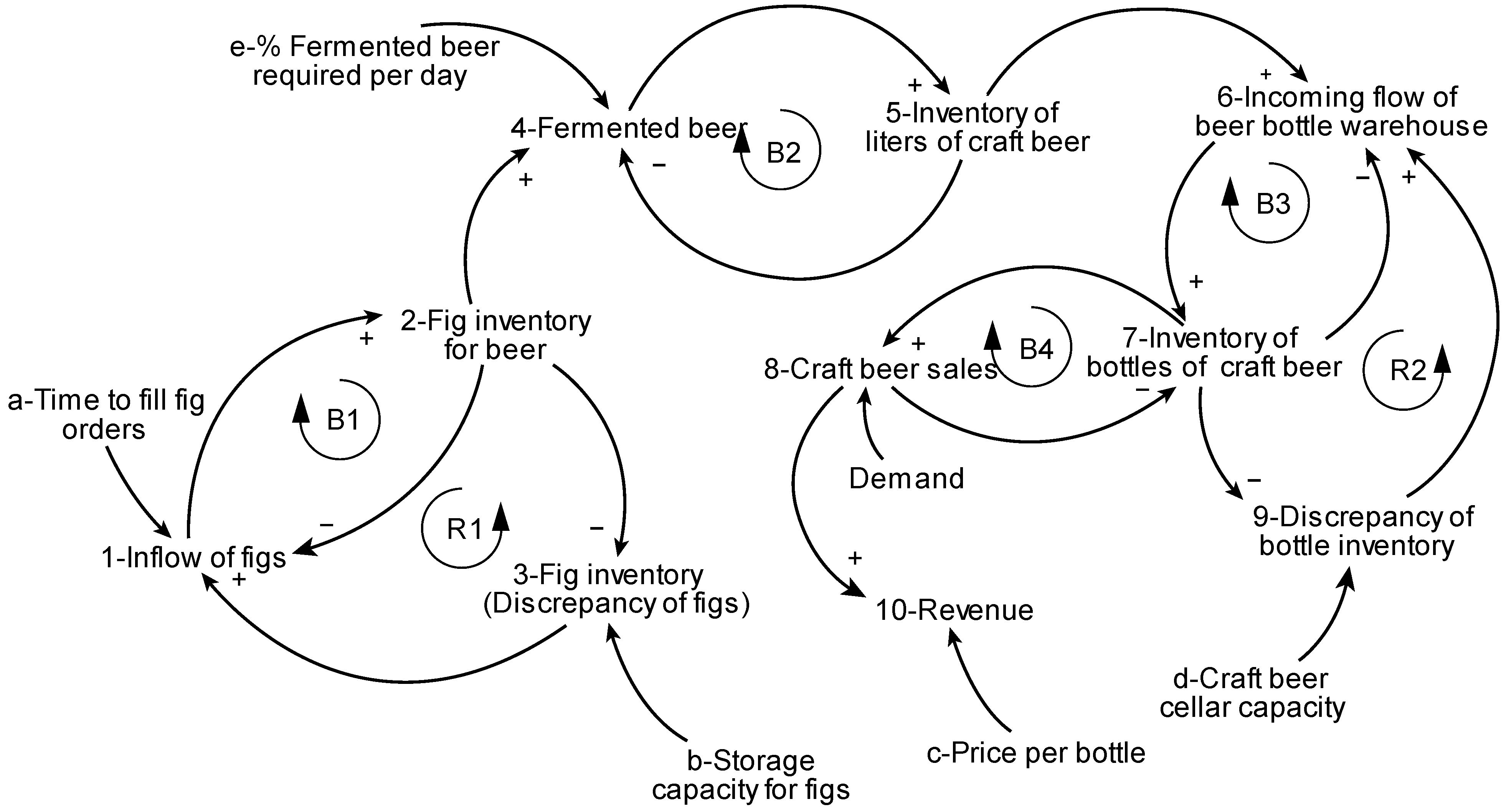
Considering the above variables, the causal model shown in Figure 1 was developed. It contains a total of six loops, with four of them of the type balance (B) and two of them of the type reinforcer (R). The variables are numbered from 1 to 10 and the parameters are identified by a letter: a, b, c, d, and e. The causal diagram’s loops are represented by R and B, which are explained as follows according to their dynamics and considering their causal relationship [28].

A causal diagram aims to graphically define the interactions and relationships between the system parameters and variables. Three types of relationships appear in the development of causal diagrams: direct relationships, simple relationships, and complex relationships. Simple relationships can take the form of a reinforcement loop (R) or a balancing loop (B). Complex relationships encompass more than two loops, which can be of type R or B. All of these types of relationships are considered in the process of constructing the causal diagram and allow us to better understand the complexity of a dynamic system.

Loop B1 captures the interactions between variables 1→2→1. This relationship acts as a balance loop as follows: if an increase in fig input due to more orders being sent to producers causes a rise in the fig inventory, the loop then produces a signal, reducing fig input with respect to warehouse capacity (parameter b—storage capacity for figs). Loop R1 considers the relationship between the three cause–effect variables 1→2→3. As fig input increases, so does the inventory, causing more figs to be required when demanded by the fermentation process (direct relationship 4). Loop B2 is composed of the variables 4→5→4. As the fermented beer quantity increases, this translates into inventory craft beer inventory (in liters). The loop is closed back to fermented beer, meaning that the amount of fermented beer transformed into inventory is subtracted from the fermented beer. Loop B3 captures the relationship between 6→7→6; as the incoming flow to the beer bottle warehouse increases, so does the inventory of bottled craft beer. Inflows are reduced in time by the effect of parameter craft beer cellar capacity.

3.3. Constructing Stock and Flow Diagrams and Their Equations

Stock and flow diagrams are rooted in the causal diagram developed in the previous stage and translated in terms of flows, as proposed by Forrester in [5]. The Forrester (flow and stock) diagrams were built from the logic of the R and B loops in the causal diagram. The Forrester diagrams encompass the stock, input and output flows, parameters, and auxiliary variables, as well as discrete elements. In our case, notice the presence of ovens for the mashing of malt and rest–fermentation, which act as delays. In our case, ovens are used to execute specific manufacturing processes (e.g., fermentation) that require a fixed time period. Figure 2 shows the complete flow and stock diagram.

The system’s equations, grouped by type (stocks, ovens, flows, and auxiliary) are presented in

Table 2. Equations of stocks, ovens, input and output flows, and auxiliary variables for craft beer production.

Stocks
Fermented beer (t) =	Fermented beer (t − dt) + (input of figs to fermentation + outflow fermentation − inflow to rest) × dt	(1)
Fig inventory for beer (t) =	Fig inventory for beer (t − dt) + (inflow of figs − input of figs to fermentation) × dt	(2)
Inventory of bottles of craft beer (t) =	Inventory of bottles of craft beer (t − dt) + (incoming flow to the beer bottle warehouse − craft beer sales) × dt	(3)
Inventory of liters of craft beer (t) =	Inventory of liters of craft beer (t − dt) + (outflow of craft beer − bottling) × dt	(4)
Wort and yeast inventory (t) =	Wort and yeast inventory (t − dt) + (inflow to wort–yeast inventory − outflow fermentation) × dt	(5)
Oven
Mashing of malt (t) =	Mashing of malt (t − dt) + (− inflow to wort and yeast inventory) × dt	(6)
Rest–fermentation (t) =	Rest–fermentation (t − dt) + (inflow to rest − outflow of craft beer) × dt	(7)
Input and Output Flow
Bottling =	Inventory of liters of craft beer × rate for bottling	(8)
Craft beer sales =	Demand × inventories of bottles of craft beer	(9)
Inflow to beer bottle warehouse =	IF the discrepancy in the bottle inventory > 0 THEN bottling × conversion of liters to bottles ELSE 0	(10)
Inflow of figs =	Fig inventory discrepancy in figs/time to fill fig orders	(11)
Inflow to rest =	Fermented beer × % fermented beer required	(12)
Input of figs to fermentation =	STEP (fig inventory for beer; resting time)	(13)
Outflow fermentation =	Wort and yeast inventory × % of must and yeast to fermentation	(14)
Auxiliary variables
Discrepancy in bottle inventory =	Craft beer cellar capacity − inventories of bottles of craft beer	(15)
Fig inventory discrepancy =	Storage capacity for figs − fig inventory for beer	(16)
Revenue =	Craft beer sales × price per bottle	(17)
Profit =	Revenue − associated costs	(18)

. Previous studies have demonstrated that the use of level and flow diagrams generates formal visual structures based on simulators producing equations representing each one of the existing relationships in the entire supply chain [29,30]. The literature review performed by Gomes Filho et al. [31] establishes a relationship between the type of supply chain and the flow of existing resources and stock accumulation.

The mathematical formulation enlarges the stock and flow diagrams to capture the system’s dynamic nature. This is why differential equations are used to represent the variation in time of the different variables. Afterward, the simulation software applies the Euler integration method to solve these equations numerically.

The equations and parameters allow for the numerical simulation of the model, and a sensitivity analysis can then be performed to evaluate pessimistic and optimistic scenarios with respect to the current situation. The numerical values used for the system parameters during the experiments are reported in

Table 3. System parameters and their numerical values.

% Inventory required = 1

% of must and yeast to fermentation = RANDOM (0.8, 1)

Conversion of liters to bottles = 2

Craft beer cellar capacity = 400

Demand = RANDOM (0.8, 1)

Price per bottle = 50

Resting time = 7

Storage capacity for figs = 1000

Time to fill fig orders = 7

Associated costs = RANDOM (0.05, 0.1) × Revenue

.

3.4. Model Validation

To validate the proposed model and its parameters, we used the percent error technique proposed by Barlas and Carpenter [16]. Essentially, this approach computes the difference between the response of a given system (in our case, the historical data of the actual plant) and the response of the simulation model when both models are submitted to the same inputs and working conditions. In particular, Barlas and Carpenter [16] suggest accepting a simulation model as a good representation of a system if the percent error between their responses is lower than 5%, where the percent error is computed as

$$percenterror=\left[\frac{simulationoutput-systemoutput}{systemoutput}\right]\times 100$$

(1)

Using the number of bottles produced as the system output, we executed several simulations and computed the percent error for each of them. In all the cases, the percent error was under the 5% limit, so we decided to accept the proposed simulation model as a good approximation of the real beer plant.

3.5. Simulation Scenarios: Sensitivity Analysis

Sensitivity analysis seeks to assess the changes in the system performance (output variables) when the values of one or several system variables are changed. Therefore, to run such an analysis, one must elect both the set of factors (or inputs) that can be controlled by the managers and that affect the set of output variables that form the system’s performance.

Concerning the output variables, which will be referred to as criteria in the following, we asked our partners to identify the system’s aspects that they consider relevant when evaluating system performance. We selected as criteria the variables in the stock and flow diagrams that relate to these aspects. It is worth noting that some of these criteria contribute to a “good” solution when they reach higher values, while others do so when their value decreases. This is why we asked the managers to, in addition to the list of criteria, indicate for each of them whether they should be “maximized” or “minimized” when looking for good solutions. Finally, as the relevance of these criteria is not homogeneous, we also required the managers to assign a weight to each criterion. The seven criteria, their optimization direction (Max for maximize and Min for minimize), and their weights are reported in

Table 4. Criteria (system outputs) used for the sensitivity analysis, their optimization direction (Max for maximize and Min for minimize), and the weights representing their relative importance.

Factors (Outputs)	Optimization Direction	Weight
Fig inventory for beer (kg)	Min	0.1
Fermented beer (L)	Max	0.1
Rest–fermentation (L)	Max	0.1
Inventory of liters of craft beer (L)	Min	0.1
Discrepancy in bottle inventory (bottles)	Min	0.15
Craft beer sales (MXN/day)	Max	0.25
Revenue (MXN)	Max	0.2

.

As per the factors (inputs), discussions with the managers in charge of the beer manufacturing process allowed for the selection of eight variables that were deemed to have the most significant impact on system output. We also defined with the plant managers each of the input variables, current (C), optimistic (O), and pessimistic (P) values, and we grouped them to form scenarios. Overall, we produced six current (C), six pessimistic (P), and six optimistic (O) scenarios. We simulated the model with the parameters and inputs’ values corresponding to each scenario and the system outputs were recorded.

The analysis of the results produced by each scenario needed to be carried out from a multiobjective perspective. To this end, we selected two well-known multicriteria decision-making (MCDM) methods: FUCA and TOPSIS [32]. The TOPSIS method first elaborates a “best” and a “worst” solution. These are not actual alternatives but rather references formed by taking the most and least favorable values of each criterion over the available set of solutions. Then, the distance between each alternative and both the best and worst solutions is calculated. The similarity ratio ($S$) of each alternative to the worst condition is computed as (distance to the worst condition/distance to the best condition + distance to the worst condition). The alternatives are ranked according to the decreasing value of $S$. The FUCA method first ranks each alternative with respect to each individual criterion, and then, it computes a weighted sum ($WS$) of the ranks obtained by each alternative.

The results produced for the seven criteria by each of the eighteen scenarios (six current scenarios, six optimistic scenarios, and six pessimistic scenarios) were analyzed using the two multicriteria methods TOPSIS and FUCA, as reported in

Table 5. Evaluation of the 18 scenarios using the TOPSIS and FUCA methods.

Scenarios	Ranking TOPSIS	$\mathit{S}$	Ranking FUCA	$\mathit{W}\mathit{S}$
Current 1	10	0.5691	12	10.55
Current 2	9	0.6009	9	8.85
Current 3	12	0.5135	10	8.95
Current 4	6	0.6410	5	8.00
Current 5	11	0.5349	14	10.8
Current 6	7	0.6295	7	8.65
Pessimistic 1	18	0.2098	18	15.00
Pessimistic 2	15	0.3289	15	11.30
Pessimistic 3	17	0.2714	16	12.30
Pessimistic 4	16	0.3138	13	10.55
Pessimistic 5	14	0.3781	17	12.60
Pessimistic 6	13	0.4333	8	8.80
Optimistic 1	3	0.6642	2	6.85
Optimistic 2	5	0.6445	11	9.70
Optimistic 3	8	0.6279	3	7.05
Optimistic 4	4	0.6522	4	7.45
Optimistic 5	1	0.7313	1	5.10
Optimistic 6	2	0.7014	6	8.50

. The TOPSIS method computed for each scenario a similarity ratio (column $S$), and then, the scenarios were sorted in decreasing order S to produce a ranking (column: Ranking TOPSYS). The FUCA method was computed for each scenario, and a weighted sum (column $WS$) of the ranks was obtained with respect to the others and for each criterion. Finally, the scenarios were sorted in decreasing order of WS to produce a ranking (column: Ranking FUCA).

The results in Table 5 show that both methods agreed on the ranking of the Optimistic 5 scenario (highlighted in bold) as the best. That said, scenario Optimistic 1, which was ranked in second and third place by FUCA and TOPSIS, respectively, seems to be a good alternative to scenario Optimistic 5. In addition, both methods agreed in considering Pessimistic 6 as the best among all of the pessimistic scenarios and Current 4 as the best among all of the current scenarios. Finally, both methods ranked the optimistic scenarios in their three best positions.

To sum up, although both methods chose scenario Optimistic 5 as the best, they ranked the other alternative scenarios differently since they computed their ranks differently. Baydaş et al. [33] compared several multicriteria methods and concluded that FUCA is very reliable, with it showing very good performance compared to other methods in the literature and particularly when the number of criteria increases.

3.6. Constructing the Graphical User Interface

The graphical user interface was built with the aim of displaying the dynamics of variables of interest according to the decision makers. A screenshot of the final interface is given in Figure 3, where the system parameters and outcomes can be seen, as well as the inventory of beer bottles with time.

The graphical user interface allows for setting specific conditions for craft beer demand (which is not constant but assumed to be random between, for instance, 94 and 100% of the nominal demand in the optimistic scenarios) and observing the actual sales which are limited by beer availability (which depends on production and stocks). Users can navigate easily from one screen to another to observe the different parts of the model and set parameters. The user interface has several buttons that allow the user to directly interact with the model on entry data. A pop-up window was added to each of these buttons to inform the user of the button’s options or purpose. The demand button can be modified directly using the mouse to modify it according to the policies mentioned. A user manual explaining all of the features of the interface was also provided to our partners.

The interface presents the system’s main outcomes at the end of the simulated period (30 days): (a) craft beer bottle inventory (215 bottles); and (b) the number of bottles required each day to increase the bottles’ inventory to capacity (400 bottles). For example, we can observe that on day 30, 185 craft beer bottles are required to increase the inventory to 400 bottles. The interface also provides the total sales value (MXN 10,100) assuming that each bottle’s sell price is MXN 50, and its production cost is 10 for each fig kg used during the process. A total profit of MXN 9930 was yielded during the 30-day simulation, and the average daily sales were 224 bottles.

This specific simulation was run assuming that daily demand varied between 94 and 100% of its nominal value. The managers suggested that daily sales of 300 bottles were very good (so the performance indicator in the interface was light green), good when they were between 160 and 299 bottles (yellow), and bad when 100 bottles or fewer were sold per day (red).

4. Discussion

The first conclusion to be drawn from the results is the confirmation of the usefulness of the system dynamics methodology in modeling complex systems. This methodology also makes it possible to simulate the dynamics of these systems and therefore anticipate their performance when different operating strategies and policies are used. Thus, the methodology can provide decision makers with precise information on the behavior of the system in the face of various situations or scenarios [4,5,9].

This methodology has already been used in the food processing sector. For example, Egea et al. [34] demonstrated that mathematical modeling and simulation made it possible to understand food processing, improving efficiency using optimization techniques based on information from relevant elements. In a context close to ours, Zamudio et al. [35] developed two dynamics models of beer fermentation; their results generated information on production capacity.

When developing the causal model for the craft beer supply chain, reinforcing and balancing loops were proposed to represent the system behavior within the system thinking framework. Dhirasasna and Sahin [36] used a multimethod approach that combined quantitative and qualitative methods to select parts of interest, identify endogenous/exogenous variables, and develop cause–effect diagrams, similar to those proposed in the present study. Similarly, Cavana and Mares [37] showed how to argue from the policy and critical thinking perspective and transformed them into a causal diagram using the tools of systems thinking and system dynamics.

Three important phases were completed to produce the final tool. First, the conceptualization of the causal model into the Forrester diagram [5]. Second, the formulation of all of the differential equations that underlie the formal model, where the flows and levels are connected [4]. Third, the definition of auxiliary variables and parameters that are directly or indirectly linked to subsequently carry out the dynamic simulation. The logic of the methodology has been described in multiple works. For instance, Angerhofer et al. [38] revised works where system dynamics had been applied to model supply chains. They provided an overview of recent research in these areas, followed by a discussion of emerging research questions and their taxonomy.

Other interesting aspects of this research are the analysis of several scenarios (optimistic and pessimistic) and the sensitivity analysis conducted [39,40,41]. Indeed, 16 scenarios were proposed and analyzed to provide decision makers with as much information as possible to support them in their decision-making processes. Moreover, two reliable multicriteria decision-making methods—FUCA and TOPSIS—were used to determine the best scenario, combining simulation and multicriteria decision making [42,43,44,45]. For instance, Luna et al. [42] used up to seven multicriteria decision-making methods (including FUCA and TOPSIS) to design optimum alembic wine distillation recipes.

In the creation of the graphical user interface, we aimed to provide users with a platform rather than a solution. This platform is a real game-changer because it will make users aware of the importance of data and will force them to carry out systematic data collection on the relevant variables of the beer craft process. Finally, we were inspired by previous works [46,47] to develop the part of the graphical interface devoted to inventories.

5. Conclusions

The alternative use of overripe products is a recurrent topic in inverse logistics when searching for sustainable options to valorize and minimize the disposal of perishable products. In this paper, we consider the use of overripe figs in the production of beer as an alternative to their disposal. Indeed, our partners (five small fig producers from Valle del Mayo in Navojoa, Sonora, Mexico) recognized that, on average, for each ton harvested, only half a ton reaches the final market while the rest loses its freshness and has to be considered as spoiled. We analyzed the complete craft beer production process to produce a simulation model using the systems dynamics approach. The resulting model was then used to evaluate different production scenarios and assess the feasibility of this new business opportunity. This project is being extended to support the future tactical and operational decisions of our industrial partners.

This study has several limitations. First, our model is based on material flows and their transformation, but it does not account for quality aspects such as the body, flavors, or color of the yielded beer. Therefore, it cannot be used to support research or decision making involving those aspects. For instance, the model is not suited to help the company’s brewmaster develop and test new receipts. Furthermore, the model behaves according to the specific recipe that our partners provided to us. Although it is possible to create a model for each potential recipe, so that the user can select the one to apply via the user interface, this has not been carried out yet. Finally, our model does not take into account the variability of the ingredients’ characteristics, and it is not able to predict how this variability might affect the actual process yield.

References

- ACERMEX (26-May-2023) Asociación de Cerveza de la República Mexicana en. Available online: https://www.thebeertimes.com/acermex-sello-cerveza-artesanal/ (accessed on 3 November 2023).
- Lagarda-Leyva, E.; Zavala, C. Plan Estratégico 2021–20226 Para la Asociación de Productores del Valle del Mayo, Navojoa, México. 2021. Available online: https://docs.google.com/presentation/d/13cjvOsP0UjP561Nv0d3tf4gqpsKgm2sn06mSSvO0uFk/edit?usp=sharing (accessed on 6 November 2023).
- Aracil, J.; Gordillo, F. Dinámica de Sistemas; Alianza: Madrid, Spain, 1997. [Google Scholar]
- Sterman, J. Business Dynamics: Systems Thinking and Modeling for a Complex World; McGraw Hill: New York, NY, USA, 2000. [Google Scholar]
- Forrester, J. Dinámica Industrial, 2nd ed.; El Ateneo: Buenos Aires, Argentina, 1981. [Google Scholar]
- Senge, P. La Quinta Disciplina, 2nd ed.; Granica: Buenos Aires, Argentina, 2005. [Google Scholar]
- Hayward, J.; Roach, P.A. Newton’s laws as an interpretive framework in system dynamics. Syst. Dyn. Rev. 2017, 33, 183–218. [Google Scholar] [CrossRef]
- Kania, J.; Kramer, M.; Senge, P. The Water of System Change. 2018. Available online: http://efc.issuelab.org/resources/30855/30855.pdf (accessed on 14 November 2023).
- Richardson, G.; Pugh, A., III. Introduction to System Dynamics Modeling with Dynamo. J. Oper. Res. Soc. 1997, 48, 1146. [Google Scholar] [CrossRef]
- Richmond, B. Introduction to System Thinking; STELLA®, Isee Systems: Lebanon, PA, USA, 2013; ISBN-10: 0970492111; Available online: https://iseesystems.com/store/books/intro-systems-thinking/ (accessed on 16 November 2016).
- Ford, D.N. A behavioral approach to feedback loop dominance analysis. Syst. Dyn. Rev. 1999, 15, 3–36. [Google Scholar] [CrossRef]
- Pastor, M.; Quecedo, M.; Merodo, J.A.F.; Herrores, M.I.; Gonzalez, E.; Mira, P.; Chen, H.; Crosta, G.B.; Lee, C.F.; Zornberg, J.G.; et al. Modelling tailings dams and mine waste dumps failures. Geotechnique 2002, 52, 579–591. [Google Scholar] [CrossRef]
- Chapra, S.; Canale, R. Numerical Methods for Engineers, 7th ed.; Mc Graw Hill Education: New York, NY, USA, 2015. [Google Scholar]
- Ghahramani, N.; Chen, H.J.; Clohan, D.; Liu, S.; Llano-Serna, M.; Rana, N.M.; McDougall, S.; Evans, S.G.; Take, W.A. A benchmarking study of four numerical runout models for the simulation of tailings flows. Sci. Total Environ. 2022, 827, 154245. [Google Scholar] [CrossRef]
- Kleijnen, J. Verification and validation of simulation models. Eur. J. Oper. Res. 1995, 82, 145–162. [Google Scholar] [CrossRef]
- Barlas, Y.; Carpenter, S. Philosophical roots of model validation: Two paradigms. Syst. Dyn. Rev. 1990, 6, 148–166. [Google Scholar] [CrossRef]
- Kleijnen, J.P.C. Sensitivity analysis and optimization of system dynamics models: Regression analysis and statistical design of experiments. Syst. Dyn. Rev. 1995, 11, 275–288. [Google Scholar] [CrossRef]
- Wang, Z.; Rangaiah, G.P. Application and Analysis of Methods for Selecting an Optimal Solution from the Pareto-Optimal Front obtained by Multi-objective Optimization. Ind. Eng. Chem. Res. 2016, 56, 560–574. [Google Scholar] [CrossRef]
- Wang, M.; Ye, C.; Zhang, D. Evaluation of Green Manufacturing Level in China’s Provincial Administrative Regions Based on Combination Weighting Method and TOPSIS. Sustainability 2022, 14, 13690. [Google Scholar] [CrossRef]
- Fernando, M.M.L.; Escobedo, J.L.P.; Azzaro-Pantel, C.; Pibouleau, L.; Domenech, S.; Aguilar-Lasserre, A. Selecting the best portfolio alternative from a hybrid multi objective GA-MCDM approach for New Product Development in the pharmaceutical industry. In Proceedings of the IEEE Symposium on Computational Intelligence in Multicriteria Decision-Making (MDCM), Paris, France, 11–15 April 2011; pp. 159–166. [Google Scholar]
- Oulasvirta, N.R.; Dayama, M.; Shiripour, M.; John, M.; Karrenbauer, A. Combinatorial Optimization of Graphical User Interface Designs. Proc. IEEE 2020, 108, 434–464. [Google Scholar] [CrossRef]
- Myers, B. Challenges of HCI Design and Implementation. ACM Interact. 1994, 1, 73–83. [Google Scholar] [CrossRef]
- Kwakkel, J.H. The Exploratory Modeling Workbench: An open source toolkit for exploratory modeling, scenario discovery, and (multi-objective) robust decision making. Environ. Model. Softw. 2017, 96, 239–250. [Google Scholar] [CrossRef]
- Kirci, M.; Isaksson, O.; Seifert, R. Managing Perishability in the Fruit and Vegetable Supply Chains. Sustainability 2022, 14, 5378. [Google Scholar] [CrossRef]
- Ojo, L.D.; Adeniyi, O.; Ogundimu, O.E.; Alaba, O.O. Rethinking Green Supply Chain Management Practices Impact on Company Performance: A Close-Up Insight. Sustainability 2022, 14, 13197. [Google Scholar] [CrossRef]
- Campuzano, F.; Mula, J. Modeling a Traditional Supply Chain by Using Causal Loop Diagrams. In Supply Chain Simulation; Springer: London, UK, 2011. [Google Scholar] [CrossRef]
- Groundstroem, F.; Juhola, S. Using systems thinking and causal loop diagrams to identify cascading climate change impacts on bioenergy supply systems. Mitig. Adapt. Strat. Glob. Chang. 2021, 26, 29. [Google Scholar] [CrossRef] [PubMed]
- Chen, H.; Yu, J.; Wakeland, W. Generating technology development paths to the desired future through system dynamics modeling and simulation. Futures 2016, 81, 81–97. [Google Scholar] [CrossRef]
- Xu, D.; Liu, E.; Duan, W.; Yang, K. Consumption-Driven Carbon Emission Reduction Path and Simulation Research in Steel Industry: A Case Study of China. Sustainability 2022, 14, 13693. [Google Scholar] [CrossRef]
- Lagarda-Leyva, E.A.; Bueno-Solano, A.; Morales-Mendoza, L.F. System Dynamics and Graphical Interface Modeling of a Fig-Derived Micro-Producer Factory. Sustainability 2022, 14, 13043. [Google Scholar] [CrossRef]
- Gomes Filho, N.; Rego, N.; Claro, J. Supply chain flows and stocks as entry points for cyber-risks. Procedia Comput. Sci. 2021, 181, 261–268. [Google Scholar] [CrossRef]
- Liu, D.; Qi, X.; Fu, Q.; Li, M.; Zhu, W.; Zhang, L.; Faiz, M.A.; Khan, M.I.; Li, T.; Cui, S. A resilience evaluation method for a combined regional agricultural water and soil resource system based on Weighted Mahalanobis distance and a Gray-TOPSIS model. J. Clean. Prod. 2019, 229, 667–679. [Google Scholar] [CrossRef]
- Baydaş, M.; Elma, O.E.; Pamučar, D. Exploring the specific capacity of different multicriteria decision making approaches under uncertainty using data from financial markets. Expert Syst. Appl. 2022, 197, 116755. [Google Scholar] [CrossRef]
- Egea, J.A.; García, M.R.; Vilas, C. Dynamic Modelling and Simulation of Food Systems: Recent Trends and Applications. Foods 2023, 12, 557. [Google Scholar] [CrossRef]
- Zamudio Lara, J.M.; Dewasme, L.; Hernández Escoto, H.; Vande Wouwer, A. Parameter Estimation of Dynamic Beer Fermentation Models. Foods 2022, 11, 3602. [Google Scholar] [CrossRef] [PubMed]
- Dhirasasna, N.; Sahin, O. A Multi-Methodology Approach to Creating a Causal Loop Diagram. Systems 2019, 7, 42. [Google Scholar] [CrossRef]
- Cavana, R.Y.; Mares, E.D. Integrating critical thinking and systems thinking: From premises to causal loops. Syst. Dyn. Rev. 2004, 20, 223–235. [Google Scholar] [CrossRef]
- Angerhofer, B.; Angelides, M. System dynamics modelling in supply chain management: Research review. In 2000 Winter Simulation Conference Proceedings (Cat. No.00CH37165); IEEE: Orlando, FL, USA, 2000; Volume 1, pp. 342–351. [Google Scholar] [CrossRef]
- Morecroft, J.D.W. System dynamics and microworlds for policymakers. Eur. J. Oper. Res. 1988, 35, 301–320. [Google Scholar] [CrossRef]
- Giannis, A.; Chen, M.; Yin, K.; Tong, H.; Veksha, A. Application of system dynamics modeling for evaluation of different recycling scenarios in Singapore. J. Mater. Cycles Waste Manag. 2017, 19, 1177–1185. [Google Scholar] [CrossRef]
- Pishghadam, H.K.; Esmaeeli, H. A system dynamics model for evaluating the firms’ capabilities in maintenance outsourcing and analyzing the profitability of outsourcing. Sci. Iran. 2023, 30, 712–726. [Google Scholar] [CrossRef]
- Luna, R.; López, F.; Pérez-Correa, J.R. Design of optimal wine distillation recipes using multi-criteria decision-making techniques. Comput. Chem. Eng. 2021, 145, 107194. [Google Scholar] [CrossRef]
- Lau, H.; Tsang, Y.P.; Nakandala, D.; Lee, C.K.M. Risk quantification in cold chain management: A federated learning-enabled multi-criteria decision-making methodology. Ind. Manag. Data Syst. 2021, 121, 1684–1703. [Google Scholar] [CrossRef]
- Varatharajulu, M.; Duraiselvam, M.; Bhuvanesh Kumar, M.; Jayaprakash, G.; Baskar, N. Multi criteria decision making through TOPSIS and COPRAS on drilling parameters of magnesium AZ91. J. Magnes. Alloys 2022, 10, 2857–2874. [Google Scholar] [CrossRef]
- Shunmugesh, K.; Panneerselvam, K. Optimization of drilling process parameters via Taguchi, TOPSIS and RSA techniques. Arch. Metall. Mater. 2017, 62, 1803–1812. [Google Scholar] [CrossRef]
- Lata, S.; Verma, H.K.; Roy, N.R.; Sagar, K. Development of greenhouse-application-specific wireless sensor node and graphical user interface. Int. J. Inf. Tecnol. 2023, 15, 211–218. [Google Scholar] [CrossRef]
- Yadav, R.; Raheman, H. Development of an artificial neural network model with graphical user interface for predicting contact area of bias-ply tractor tyres on firm surface. J. Terramech. 2023, 107, 1–11. [Google Scholar] [CrossRef]