Numerical Simulations of Failure Mechanism for Silty Clay Slopes in Seasonally Frozen Ground

Abstract

Landslide damage to soil graben slopes in seasonal freezing zones is a crucial concern for highway slope safety, particularly in the northeast region of China where permafrost thawing is significant during the spring. The region has abundant seasonal permafrost and mostly comprises powdery clay soil that is susceptible to landslides due to persistent frost and thaw cycles. The collapse of a slope due to thawing and sliding not only disrupts highway operations but also generates lasting implications for environmental stability, economic resilience, and social well-being. By understanding and addressing the underlying mechanisms causing such events, we can directly contribute to the sustainable development of the region. Based on the Suihua–Beian highway graben slope landslide-management project, this paper establishes a three-dimensional finite element model of a seasonal permafrost slope using COMSOL Multiphysics 6.1 finite element numerical analysis software. Additionally, the PDE mathematical module of the software is redeveloped to perform hydrothermal-coupling calculations of seasonal permafrost slopes. The simulation results yielded the dynamic distribution characteristics of the temperature and seepage field on the slope during the F–T process. The mechanism behind the slope thawing and sliding was also unveiled. The findings provide crucial technical support for the rational analysis of slope stability, prevention of sliding, and effective control measures, establishing a direct linkage to the promotion of sustainable infrastructure development in the context of transportation and roadway engineering.

1. Introduction

The freezing and thawing (F–T) of soil will lead to changes in its physical and mechanical properties, and foreign scholars have conducted a lot of research on the mechanical properties of soil under freeze–thaw conditions. In 2011, Zhu [1] investigated the dynamic properties of frozen clay in the perennial permafrost roadbed of Beiluhe of the Qinghai–Tibet Railway. It was found that the maximum dynamic shear modulus of frozen clay decreased with the increase in temperature and the decrease in surrounding pressure, and the reference shear strain value decreased with the increase in temperature and surrounding pressure and the decrease in water content. In 2012, Tang et al. [2] studied the variation rule of the freezing strength and temperature of Shanghai mud clay; in the early stage of freezing, the strength of the frozen mud clay increased to the maximum value with time, and it increased with the decrease in temperature. In 2015, Ling [3] conducted a low-temperature cyclic triaxial test on frozen compacted soil in Nehe, Heilongjiang Province, and found that the freeze–thaw process had a significant effect on the dynamic shear modulus and damping ratio of the soil. In 2019, Lv et al. [4] analyzed the effects of the water content, freezing temperature, and freeze–thaw cycle time on shear strength by using cohesion and the internal friction angle as the shear strength indexes, and they analyzed the effects of the water content, freezing temperature, and freeze–thaw cycle time by combining them with the grey theory, and the results showed that the water content has the greatest effect on the cohesion and the angle of internal friction, and the angle of internal friction and the cohesion within the range of the plastic limit to the liquid limit decrease with the increase in the water content. Chen et al. [5] investigated the strength characteristics of unsaturated powdery clay after cooling and a single freeze–thaw cycle using a GDS triaxial test system after controlling the initial matrix suction, and the results showed that the initial matrix suction freezing process can enhance the shear strength of the soil body, so that the stress–strain curves of the soil body show certain strain-hardening characteristics at different temperatures. Hu et al. [6] found that the stress–strain curves of the original soil specimens were characterized by strain hardening with shear shrinkage by conducting a freeze–thaw cycle and consolidation-drainage triaxial tests on pulverized clay, and that the perimeter pressure during consolidation and the triaxial loading stages attenuated the adverse effects of the freeze–thaw cycle. Chen et al. [7] found that the freezing temperature and the number of freeze–thaw cycles had a significant effect on the axial strain of the pulverized clay under cyclic loading. In 2022, Zhou et al. [8] considered the effect of F–T to carry out static mechanical property tests on basalt-fiber and basalt-powder-modified powdered clay; after 30 cycles of F–T, the shear strength of the two kinds of modified powdered clay were higher than that of the unamended powdered clay, and the effect of basalt fibers on the reinforcement of this increase was generally better than that of basalt powder, which provides some theoretical references to the practical engineering in seasonal permafrost areas. Xu et al. [9] carried out electron microscopy (SEM) and CT scanning on the pulverized clay after freeze–thaw cycles. After continuous F–T, the internal microstructure of the pulverized clay became looser, the pores and connections between soil particles deteriorated, and the shear strength, elastic modulus, and cohesion decreased and stabilized with the increase in the number of cycles.

The research on seasonal permafrost in China has developed relatively rapidly. Song et al. [10] conducted freeze–thaw cycle tests on loess in Lanzhou, and the test results showed that with the increase in the temperature gradient under the same dry bulk weight, the decrease in the consolidation pressure in the early stage of the soil after multiple freezes and thaws gradually decreased, and the decrease in cohesion increased. Wang [11] and others conducted compression tests and drainage shear consolidation tests on in situ soils and unfrozen soils under different freeze–thaw conditions, respectively. The results show that the compression ratio of clay after F–T is higher than that of in situ soil and that F–T has a bi-directional effect on remolded soils with different dry densities, decreasing the compressibility of loose lumpy soils with low densities, and increasing the compressibility of dense, high-density soils. Qi [12] believes that the strength theory of thawed soil is used in the study of permafrost strength, it is difficult to reflect the compression and thawing phenomenon of soil under high stress, and the establishment of the ontological relationship of permafrost is mainly based on empirical formulas and focuses on the study of creep, which needs to be further improved. Based on the theory of significance analysis, Chang et al. [13] investigated the significant effects of the number of freeze–thaw cycles, freezing temperature, enclosing pressure, and the interactions among the factors on the mechanical properties of pulverized sandy soils. The results of the study show that the perimeter pressure and the number of F–T cycles have a strong effect on the mechanical properties of chalky sand, while the freezing temperature has little effect, and the combined interaction of freezing temperature with the number of F–T cycles has a great effect on the mechanical properties of chalky sand. Zheng [14] studied the changes of soil particles and soil pores in the process of a freeze–thaw cycle using the relevant mechanical tests of soil, and found that the particles of soil will be gradually ruptured after many times of F–T, which will lead to a gradual increase in the specific surface area of the soil and the bounding water content. Hu et al. [15] conducted a triaxial shear test in order to elucidate the effect of cooling temperature on the freeze–thaw cycle effect of soil. The results showed that freezing and freeze–shrinkage coexisted during soil freezing, and the deformation of both increased with the decrease in the cooling temperature. The lower the cooling temperature, the smaller the range of variation in damage strength with the number of freezes and thaws and the number of freezes and thaws required to reach a new steady state, and the weaker the cumulative effect of the freeze–thaw cycles.

The study of slope stability has always been a more complex problem, and research scholars at home and abroad have conducted more detailed studies on slope failure and instability problems, and have achieved many fruitful results. However, for the study of landslides on powdery clay slopes in the Quaternary freezing zone, relying only on traditional analytical methods can no longer meet requirements due to the complex coupling of the hydrothermal multiphysical fields involved. The damage problem of seasonal permafrost zone slopes mainly originates from the freeze–thaw damage caused by the cold environment, and its thaw–sliding mechanism is different from that of the non-permafrost-zone slopes, and the resulting sliding surfaces are not the circular sliding surfaces in the traditional sense, but rather in the form of shallow landslides. Shallow landslides are distributed in many parts of the world, and

Table 1. Shallow landslides around the world.

First Author/Year of Publication	Research Area	Type of Landslide
Rogers 1980	North island	Slide
Lim 1996	-	Earth flow
Pasuto 1998	Veneto	Soil slip
Eigenbrod 1999	Ontario	Shallow translational and rotational
Shakoora 2005	Ohio	Shallow translational and rotational
Gullà 2004	Calabria	Soil slip
Claessens 2007	North island	Earth flow
Dahal 2009	Shikoku island	Shallow landslides
van Asch 2009	Emilia-Romagna	Soil slip

summarizes some of the representative research literature on shallow landslides [16,17,18,19,20,21,22,23,24], which shows that the research on shallow landslides started late and the research power is weak. Scholars have given different definitions of shallow landslides according to different research disciplines and research purposes, and generally defining the rapid destruction of shallow slopes as soil sliding, earth flow, and shallow advection is also more commonly used. However, no matter which definition, these landslides have the following common characteristics: small volume of landslides, a depth of the slip surface between 1 and 5 m, and some scholars define shallow as within 10 m. In northeastern China, due to the spring temperature rise, they began to enter the thawing stage, the slope surface’s soil began to melt, while the bottom of the slope soil is still in a frozen state, the unthawed soil layer plays a similar role as a water blocker; the water flow effect, cannot be ejected in a timely way from the slope, reducing the strength of the shallow soil on the slope surface, leading to the slope having its own gravity for thawing and sliding, and the slide surface is mostly of a flat and straight type.

Based on the above analysis, this study is based on the road graben slope landslide management project along the Suihua–Beian Expressway in Northeast China; firstly, the secondary development of PDE equations in comsol software is carried out, and the water–heat–force coupling model of the slope is established by combining the relevant local climatic and hydrogeological data, and then the distribution of the temperature, moisture, and stress of the slope in the freezing and thawing periods is detailed. Secondly, the distribution of temperature, moisture, stress, etc., of the slope during the freezing and thawing periods was elaborated, and, based on which, the intrinsic mechanism of the shallow landslide on the slope during the spring thawing period in seasonal permafrost areas was finally analyzed.

2. Finite Element Modeling of Slopes

2.1. Theoretical Governing Equations of Hydrothermal Coupling Research

The coupled hydrothermal equation involved in the numerical simulation of slopes is a fully coupled equation, which is the focus of the calculation. It is essential to establish the basic assumptions before modeling. In order to make the model calculations operable, appropriate simplifications are made to ensure the accuracy of the calculation results, and the basic assumptions are as follows: (1) the slope soil material is regarded as a homogeneous linear elastic material; (2) the compression and expansion of ice, water, and soil affected by freezing and thawing are not taken into account, and the density is set to a constant; (3) the solid model of the soil is chosen to be isotropic, and the water and thermal parameters such as diffusion coefficients are consistent in all directions in the model; (4) the water seepage inside the soil body satisfies the generalized Darcy’s law, and the water migration is of liquid water migration without considering the form of gaseous water; (5) the moisture of the soil body in the model is assumed to be distilled water, ignoring the effects of ionic transformations and the salt content on the migration of water, and the difference in the distribution of temperature and moisture of the soil body at the same horizontal depth is not taken into account.

2.1.1. Controlling Equations for the Seepage Field

The partial differential equations used in the numerical simulation of slopes are set up according to the laws of conservation of mass and energy. The controlling equations for the moisture field required by the model are mainly derived from the mass-conservation equation, which is now analyzed for a microcell. The essence of mass conservation is that the moisture content entering the microcell from the outside is equal to the sum of the ice and unfrozen water content inside the microcell within a period of time, i.e., the moisture entering the microcell from the outside is converted into the ice in the pore space of the internal microcell and the unfrozen water. Assuming that the differential unit cell is a rectangle with dimensions of length Δx, width Δy, and height Δz, let the migration velocity of water inside the microelement be υ, which represents the amount of water that passes through the microelement per unit of time, and the migration velocity of the water flowing into the microelement in the direction of the x-ax is υ_x. Therefore, the amount of moisture change per unit of time along the x-axis direction of the differential cell is established according to the following equation.

$$\Delta m_X={\rho }_l({\nu }_X+\frac{\partial {\nu }_X}{\partial x}\Delta x-{\nu }_X)\Delta y\Delta z={\rho }_l\frac{\partial {\nu }_X}{\partial x}\Delta x\Delta y\Delta z$$

(1)

Along the above lines, it is found that the change in moisture per unit of time of the microelement along the direction of the y and z axes is as follows:

$$\Delta m_y={\rho }_l({\nu }_y+\frac{\partial {\nu }_y}{\partial y}\Delta y-{\nu }_y)\Delta x\Delta z={\rho }_l\frac{\partial {\nu }_y}{\partial y}\Delta y\Delta x\Delta z$$

(2)

$$\Delta m_z={\rho }_l({\nu }_z+\frac{\partial {\nu }_z}{\partial z}\Delta z-{\nu }_z)\Delta x\Delta y={\rho }_l\frac{\partial {\nu }_z}{\partial z}\Delta y\Delta x\Delta z$$

(3)

Thus, the overall moisture change in the micrometabolite per unit of time is as follows:

$$\Delta m={\rho }_l(\frac{\partial {\nu }_x}{\partial x}+\frac{\partial {\nu }_y}{\partial y}+\frac{\partial {\nu }_z}{\partial z})\Delta x\Delta y\Delta z$$

(4)

The overall amount of moisture change in a micrometabolite is attributed to the sum of the change in its internal unfrozen water content and its pore ice content as follows:

$$\Delta m=\frac{\partial ({\rho }_l{\theta }_l+{\rho }_i{\theta }_i)}{\partial t}\Delta x\Delta y\Delta z$$

(5)

where θ_l(%) is the volume content of unfrozen water; θ_i(%) is the volume content of pore ice. Combine Formulas (4) and (5), and in order to make the formulas simpler and clearer, the partial differential in the formulas can be expressed using the Hamiltonian operator:

$$\nabla \nu =\frac{\partial {\theta }_l}{\partial t}+\frac{{\rho }_i}{{\rho }_l}\frac{\partial {\theta }_i}{\partial t}$$

(6)

Formula (6) is the standard form obtained according to the law of conservation of mass, and in order to establish the relationship between the rate of water migration and the unfrozen water content and the internal potential energy of the soil, according to the generalized Darcy’s law, we use the equation

$$\nu =k({\theta }_l)[\frac{\partial (\phi )}{\partial x}+\frac{\partial (\phi )}{\partial y}+\frac{\partial (\phi )}{\partial z}]=k({\theta }_l)\nabla (\phi )$$

(7)

Assume that the matrix potential is φ_m, the gravitational potential φ_g = z. This is obtained by substituting it into Formula (7):

$$\nu =k({\theta }_l)\nabla ({\phi }_m+z)=k({\theta }_l)\nabla ({\phi }_m)+k({\theta }_l)$$

(8)

By substituting Formula (8) into Formula (6), the control equation for the seepage field in the final hydrothermal-coupling differential formula can be obtained as Formula (9):

$$\nabla [k({\theta }_l)+\nabla ({\phi }_m)]+\nabla [k({\theta }_l)]=\frac{\partial {\theta }_l}{\partial t}+\frac{{\rho }_i}{{\rho }_l}\frac{\partial {\theta }_i}{\partial t}$$

(9)

2.1.2. Controlling Equations for the Temperature Field

Hydrothermal-coupled differential equations in the temperature control equation derivation of the idea is in accordance with the law of the conservation of energy; similar to the idea of the conservation of mass analysis, with the same differential unit as the object of the study, we can consider a micro-element body within the temperature change and the phase change of the sum of the energy is the amount of heat transported into the micro-element body. Assuming that the heat flux is q, the amount of heat entering the microcell along the x-axis in a unit of time is

$$\Delta Q_x=(q_x+\frac{\partial q_x}{\partial x}\Delta x-q_x)\Delta y\Delta z=\frac{\partial q_x}{\partial x}\Delta x\Delta y\Delta z$$

(10)

Similarly, the heat entering the microelement body along the y and z axes per unit of time can be found using

$$\Delta Q_y=(q_y+\frac{\partial q_y}{\partial y}\Delta y-q_y)\Delta x\Delta z=\frac{\partial q_y}{\partial y}\Delta x\Delta y\Delta z$$

(11)

$$\Delta Q_z=(q_z+\frac{\partial q_z}{\partial z}\Delta z-q_z)\Delta x\Delta y=\frac{\partial q_z}{\partial z}\Delta x\Delta y\Delta z$$

(12)

Thus, the overall energy change per unit of time into the micrometabolite is

$$\Delta Q=(\frac{\partial q_x}{\partial x}+\frac{\partial q_y}{\partial y}+\frac{\partial q_z}{\partial z})\Delta x\Delta y\Delta z=\nabla (q)\Delta x\Delta y\Delta z$$

(13)

The flow of heat is rewritten as an equation related to thermal conductivity, which is the following formula:

$$q=\lambda (\frac{\partial T}{\partial x}+\frac{\partial T}{\partial y}+\frac{\partial T}{\partial z})=\lambda \nabla (T)$$

(14)

Formula (14) is then substituted into Formula (13) to obtain the energy imparted to the micrometabolite per unit of time:

$$\Delta Q=\nabla [\lambda \nabla (T)]\Delta x\Delta y\Delta z$$

(15)

Again, because the sum of the energy of the temperature change generated inside the microelement and the phase transition is equal to the heat transferred into the microelement, we find

$$\Delta Q=(C\frac{\partial T}{\partial t}-L{\rho }_i\frac{\partial {\theta }_i}{\partial t})\Delta x\Delta y\Delta z$$

(16)

The temperature field control equation in the hydrothermal-coupling equation can be obtained by combining Formulas (15) and (16) as the following Formula (17):

$$C\frac{\partial T}{\partial t}-L{\rho }_i\frac{\partial {\theta }_i}{\partial t}=\nabla [\lambda \nabla (T)]$$

(17)

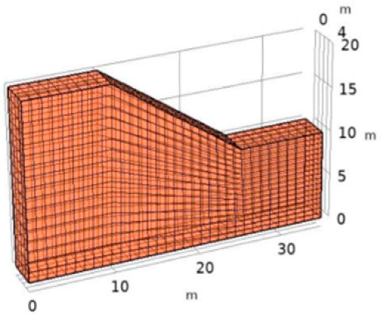
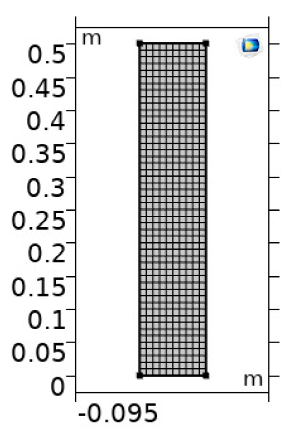
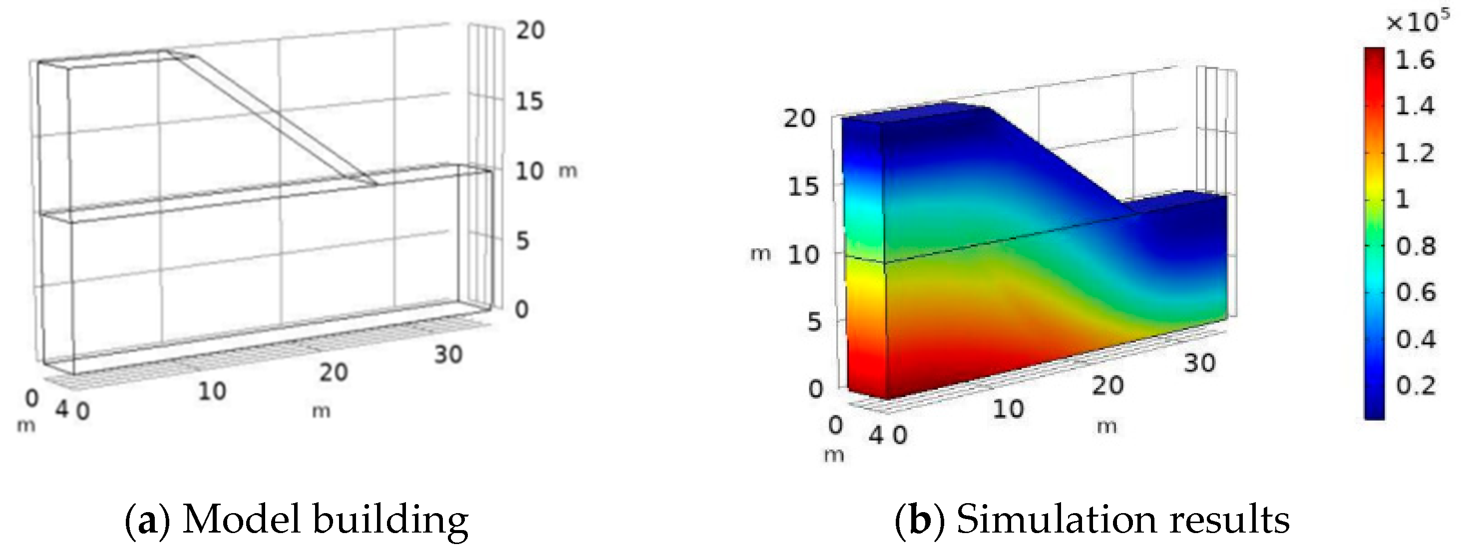
2.2. Geometric Modeling and Meshing

According to the actual site structure of the landslide slope at the test section K44+000 of Suihua–Bei’an Expressway, the hydrothermal finite element numerical model of the slope in seasonal permafrost area is established, and most of the soils at the slope in the Suibei area consist of low-liquid-limit pulverized clay, and in order to simplify the calculations, the model involves the height of the soils as foundations. The thickness of the slope as a whole is 4 m, and the geometric model of the slope constructed is 3D. As shown in Figure 1, the meshing of the slope model adopts the mapping and sweeping method, setting the front face of the slope as the source face and the back face of the slope as the target face, and the two faces are swept linearly. The approach of sweeping is to generate hexahedra and then map each other to form the mesh, and in order to improve the accuracy of the model computation, the overall size of the mesh is ultra-detailed. The maximal cell size of the mesh is 1.23 m, and the minimum cell size is 0.0525 m. The maximum cell growth rate, curvature factor, and resolution of the narrow region are 1.35, 0.3, and 0.85, respectively.

2.3. Model Parameter

The parameters chosen for this study are predominantly derived from the customary empirical values laid down in the Design Code for Foundations of Buildings in Permafrost Areas (JGJ118-2011) [25] and the empirical data ascertained through a series of experiments conducted by Xu and other scholars [26]. The numerical calculation model for slopes in seasonal permafrost regions demonstrates the specific parameters, which are presented in

Table 2. Table of model parameters.

Parameter	Notation	Numerical Value
Specific heat capacity of liquid water	cl	4.18 kJ/(kg·K)
Specific heat capacity of ice	ci	2.09 kJ/(kg·K)
Thermal conductivity of water	λl	0.58 W/(m·K)
Thermal conductivity of ice	λi	2.32 W/(m·K)
Latent heat of ice–water phase transition	L	334.5 kJ/kg
Density of ice	ρi	900 kg/m3
Density of water	ρl	1000 kg/m3
Soil density	ρs	1550 kg/m3
VG model parameters	n	4.2
VG model parameters	m	0.76
VG model parameters	a0	0.02
Ice content factor	a	0.5
Pore ice impedance factor	w	5
Saturated volumetric water content of soil	θm	0.45
Soil residual volumetric water content	θn	0.04
Saturated coefficient of permeability of soil	ks	1 × 10−7 m/s
Specific heat capacity of frozen soil skeleton	csf	0.53 kJ/(kg·K)
Specific heat capacity of the soil melting skeleton	csu	0.76 kJ/(kg·K)
Thermal conductivity of soil skeleton	λs	1.95 W/(m·K)
Freezing temperature of the soil	Tf	−0.54 [°C]
Young’s modulus of soil	E	25 [MPa]
Poisson’s ratio of soil	υ	0.3

.

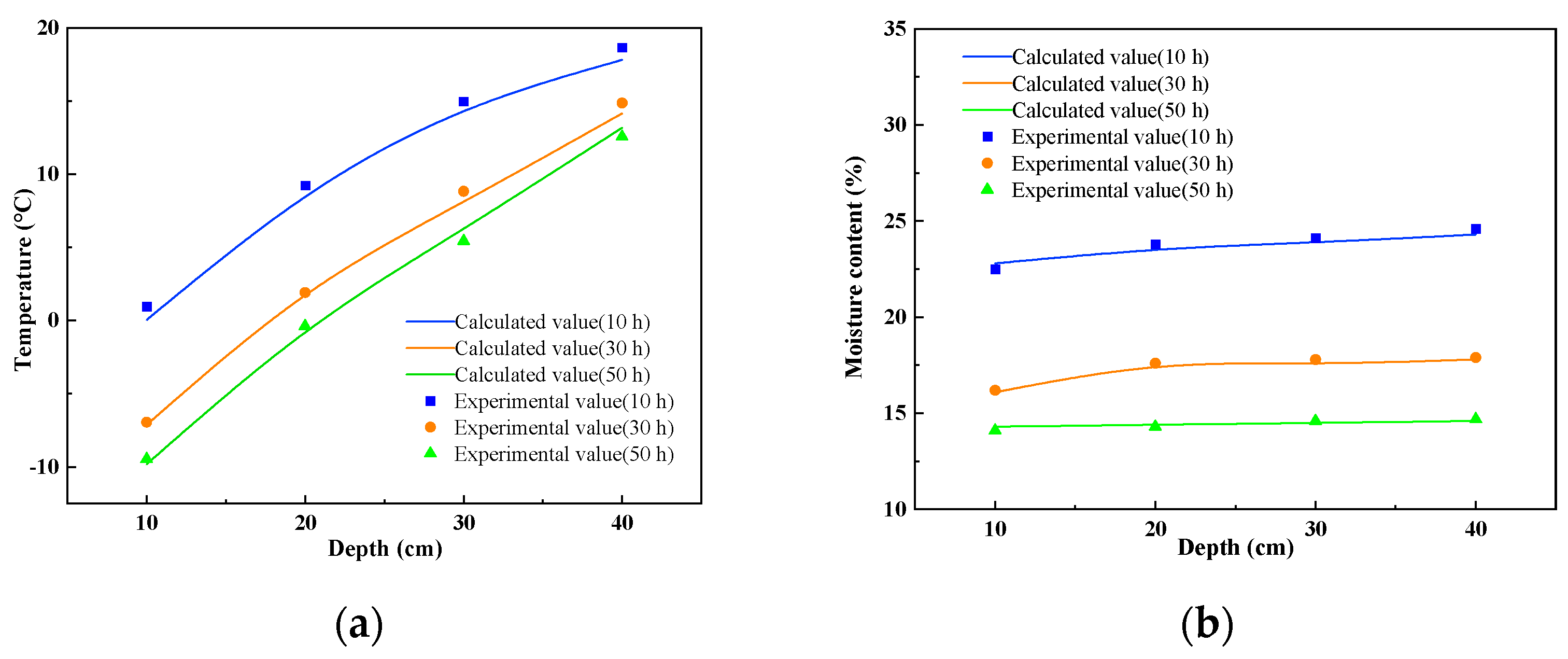
2.4. Validation of the Correctness of the Numerical Simulation Method

In order to verify that the numerical simulation method proposed in this paper is correct and feasible, with reference to the one-dimensional soil column unidirectional freezing test accomplished by Cui [27], the freezing of the soil column is numerically simulated using the method of hydrothermal coupling as described above, and then the results obtained from the calculations are compared with the results of the freezing test. As shown in Figure 2, the geometry of the soil column model is a rectangular two-dimensional cross-section of 10 cm × 50 cm, and the meshing is completed with mapping, and the cells are of the free quadrilateral type.

The initial and boundary conditions of the soil column model and the relevant physical and mechanical parameters of the soil used are all from the original settings. The temperature boundary conditions of the model are the temperature of the upper boundary, i.e., the temperature of the cold end, is set to −20 °C; the temperature of the lower boundary; and the temperature of the whole soil column, which is set to an initial temperature of 20 °C. The two sides of the boundary are zero-flux adiabatic boundaries; the moisture boundary conditions are the whole surrounding of the model, which is set to be a water-insulated condition, without considering the external environment. The moisture boundary conditions are the whole model, which is set to be surrounded by a water barrier condition, without considering the infiltration of external water, and the initial volumetric water content of the soil is set to 32%. As shown in Figure 3 below, the hydrothermal dynamic distribution of the soil column at different times was obtained using a COMSOL calculation.

In order to judge the accuracy and rationality of the calculation results more intuitively, the temperature and water content results calculated using the model and the hydrothermal data obtained from the test are organized and merged into a graph, as shown in Figure 4. As can be seen from the figure, the results obtained using the hydrothermal-coupling-calculation method in this paper tend to be consistent with the change rule of hydrothermal law in the test results: the soil body increases in the process of freezing; the temperature, with the gradual increase in time and depth, constantly increases; the unfrozen water content gradually increases in depth, and constantly become greater; and with the increase in time and constant decrease in depth, the water constantly moves from the unfrozen area to the frozen area. Therefore, the simulation effect using the numerical simulation method in this paper is better and can be used for the subsequent calculation of slope water–heat coupling.

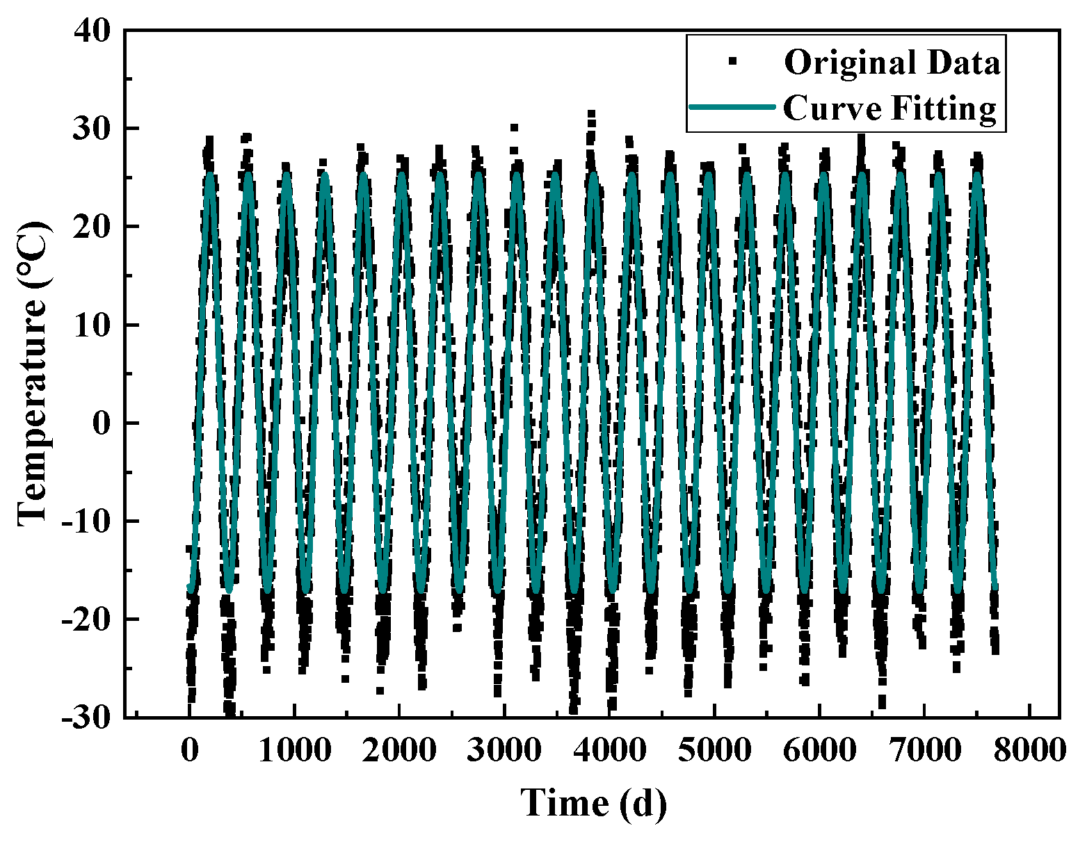
2.5. Boundary and Initial Conditions

The boundary condition setting of slopes in a seasonal permafrost region is one of the important steps in model calculation, which involves complicated hydrothermal boundary conditions, and in order to accurately obtain the dynamic change law of a slope hydrothermal field, it is necessary to reasonably set the corresponding model boundary conditions. In order to facilitate the calculation, the upper boundary of this paper includes the top of the upper slope, the slope surface, and the bottom of the slope, which are set up using the first type of thermal boundary; the specific functional form is based on the meteorological data of the Suibei area in the past 10 years, as shown in the finalized Figure 5 fitting. The foundations under a certain depth have little change in their temperature and are in a constant-temperature zone, so the lower boundary temperature of the model is set to be 7 °C through combining the results of the investigation of the seasonal freezing zone by Zhang [28]. The whole range of the slope is large, and the effect of the temperature boundary around the model on the internal temperature can be ignored through setting up an adiabatic setup around the periphery and treating it as a zero flux of heat. Considering that the local water table is not high, and in order to reduce the complexity of the model calculation, this paper only considers the influence of the change in the water content of the slope soil itself during the freeze–thaw process on the hydrothermal field. The upper boundary moisture condition of the model is determined by referring to the research results of Lin [29] and combining them with the actual situation in the field, and the lower boundary of the moisture field is set in the form of a fixed moisture content, which is consistent with the initial moisture content set by the foundation. Formulas (18) and (19) are the specific time functions of temperature and moisture at the upper boundary of the slope model. The stress boundary conditions of the slope model are adopted as the basic settings in the solid mechanics module, and the whole slope is assumed to have no displacement in the horizontal direction and to only generate displacement in the vertical direction, with the upper boundary as a free boundary, the lower boundary as a fixed constraint, and the model surrounded by a roll support.

$${\mathrm{T}}_{\mathrm{t}}=4.5+30\mathrm{s}\mathrm{i}\mathrm{n}(\frac{\mathsf{\pi }}{183}(\mathrm{t}+17))$$

(18)

$${\mathrm{U}}_{\mathrm{t}}=0.28+0.07\mathrm{s}\mathrm{i}\mathrm{n}(\frac{\mathsf{\pi }}{183}(\mathrm{t}+17))$$

(19)

where T_t and U_t are the temperature and moisture at the upper boundary, respectively. The local air temperature of 4.5 °C at the beginning of April is used as the starting value in the temperature boundary function, and the initial moisture content of the slope is used as the starting value for the volumetric moisture content.

The temperature and moisture levels in the longitudinal direction vary across different depths of the entire model. For ease of calculation, the model is initially separated into two parts: the slope body and the foundation, depicted in Figure 6. Taking into account the present meteorological conditions in Suihua, the upper slope body’s initial temperature is fixed at 15 °C with an initial moisture content of 28%. Meanwhile, the lower foundation’s initial temperature is 7 °C, with an initial moisture content of 30%. The paper’s slope geometry is founded on the actual slope existence, which develops through continuous gravitational deformation. Hence, prior to conducting subsequent stability studies and analyses, the initial ground stress balance is crucial. Figure 5 exhibits the use of the solid mechanics module to equilibrate the calculated stress as the initial stress value for subsequent simulations.

3. Simulation Results and Analysis

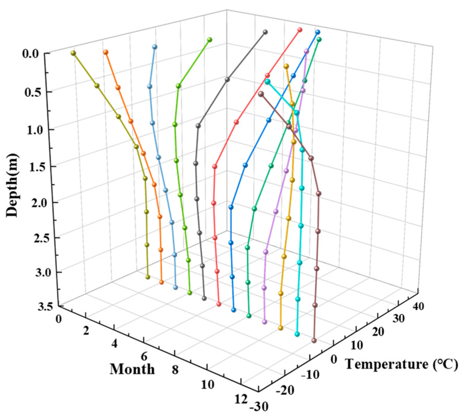
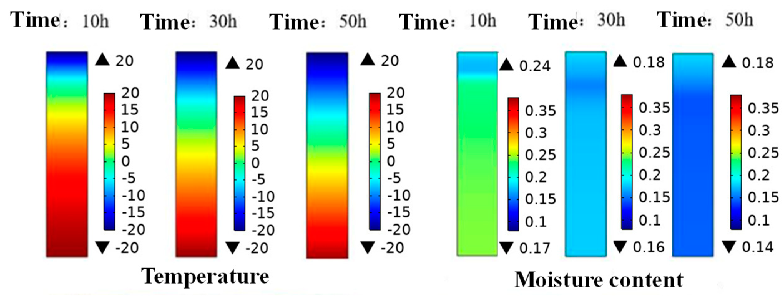
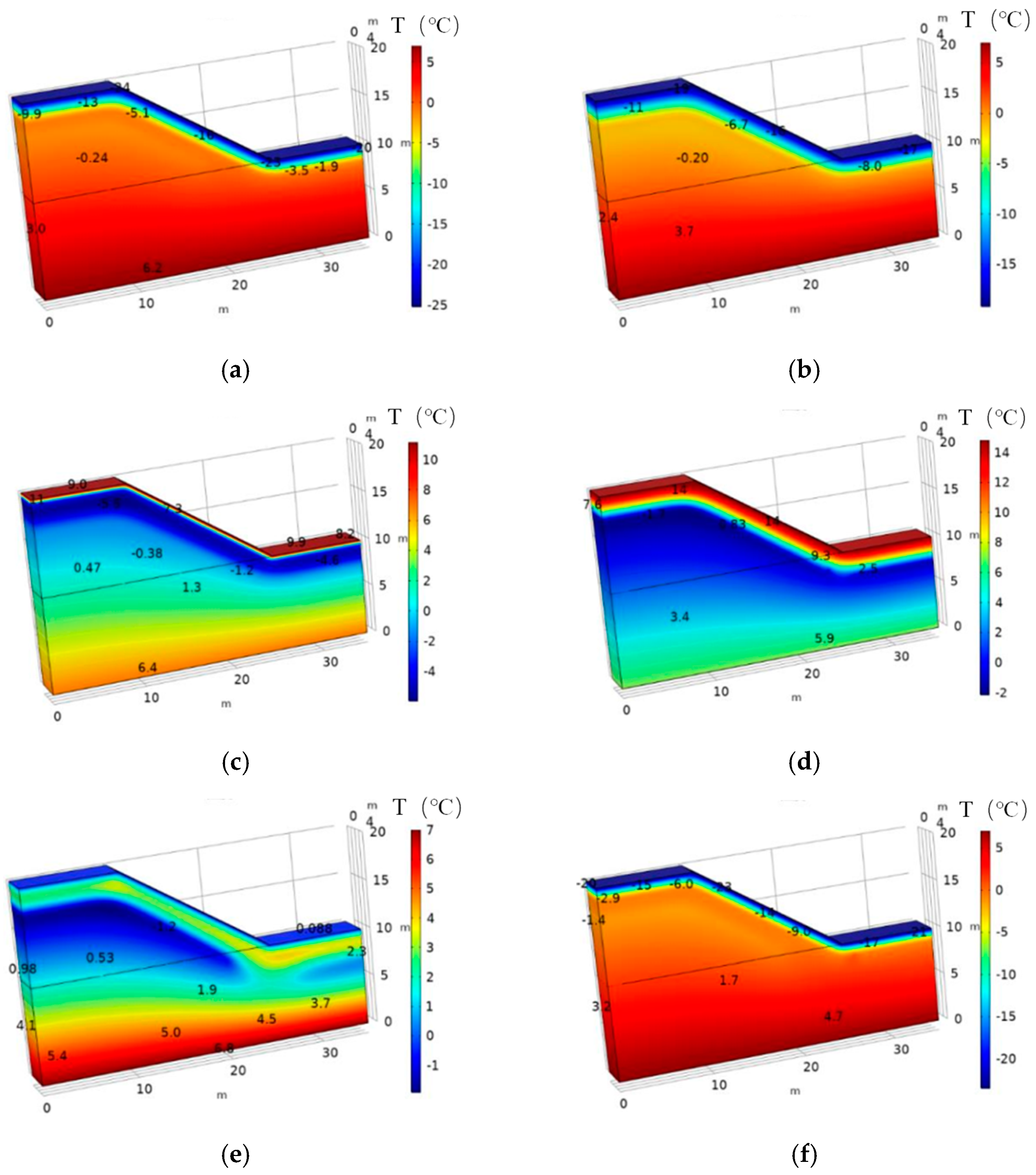
3.1. Temperature Variations under F–T Conditions

Figure 7 shows the temperature field distribution of the slope over a year; the right side of the figure shows the temperature legend, grid scale for the model’s geometric size. The temperature field distribution of the cloud can be seen in the upper boundary surface temperature of the slope over the year, from January to March for the negative temperature, from April to September for the positive temperature, and from October to December for the negative temperature. In October, the upper surface temperature of the slope reached −1 °C, which is the beginning of soil freezing, and then as time goes on, the outside temperature is gradually reduced causing the soil temperature to lower and the upper shallow layer of the slope to form part of the frozen soil layer. The upper surface of the slope in January reached a minimum temperature of −25 °C, which is the end of the soil freezing stage. In February, the upper surface temperature of the slope began to increase, indicating that this is the beginning of the soil-melting stage, and then, with the gradual increase in outside-air temperature, the upper surface temperature of the slope gradually rebounds. The 0 °C isotherm is gradually moved down, indicating that the depth of melting is constantly increasing, so the upper surface temperature of the slope in April is back above 0 °C, indicating that the surface layer of the frozen soil has been completely melted at this time, indicating the end of the melting period and the frozen soil layer. In the slope soil from February to April, this melting stage, which is the spring melting period, can see a soil temperature with an increase in vertical depth. With an increasing depth, the ground extends downward to 3.5 m. The temperature of the soil body basically remains constant, which indicates that the outside temperature mainly affects the slope inside a certain level of soil temperature; the temperature of the deeper layers of the soil body is less impacted.

From the temperature distribution of the above cloud diagrams and the analysis, it can be concluded that in the seasonal permafrost region slope soils affected by F–T are mainly concentrated in the shallow layer of the surface, and the temperature fluctuation range of the slope soils with a longitudinal depth of more than 4 m in the spring thawing period is not large. Therefore, the surface soil of the slope surface was taken as the object of the study, and the center point of the slope surface was taken as the starting point, and the sample points were set every 0.5 m along the interior in the direction of the perpendicular slope surface. Taking an average of eight sample points from 0 m to 3.5 m, we take each sample point from the results of the temperature field calculations to find the corresponding soil sample temperature data, and then all the acquired sample temperature data will be organized and plotted, as shown in Figure 8.

As can be seen from Figure 8, the temperature of the slope soil was related to the level of depth throughout the freeze–thaw process. During the period from March to September, the temperature of the soil body of the slope showed a tendency to decrease and then increase with increasing depth; from October to December, the temperature of the soil body of the slope increased and then decreased with the increasing depth; and the temperature of the soil body of the slope gradually increased with increasing depth during the period from January to February. This is found because in the slope in the freezing stage, due to the low temperature of the external environment caused by the low temperature of the surface layer of the soil, to the thawing stage, the external environment temperature continues to rise as well, as does the temperature of the soil in the deeper layer of the soil body, which still maintains a higher temperature. The temperature is higher than the temperature of the soil body during the freezing stage, so due to the formation of a difference in the temperature gradient, the transfer of heat will move from the region’s area of high temperature to the region of low temperature through a gradual transition, which led to the formation of the phenomenon described above. In the area of the slope within 2 m of the slope surface, the temperature fluctuation of the soil is more intense, while in the area deeper than 2 m, the temperature change of the soil is smaller, which indicates that the shallow soil layer of the slope is more affected by the temperature of the external environment, and the deeper soil layer is less affected by the temperature of the external environment. In addition, during the freezing stage of the slope, the freezing line, i.e., the 0 °C temperature contour, moved downward with the gradual decrease in the external ambient temperature, indicating that the freezing depth gradually increased until it moved to the maximum depth of about 2.3 m in March. The temperature in the area 2 m from the surface of the slope body warmed up to a positive temperature in April, and the surface permafrost had completely melted, with a depth of about 1.5 m. The freezing line was also moved downward with the gradual decrease in the external ambient temperature, indicating that the freezing depth gradually increased until it moved to the maximum depth of about 2.3 m in March.

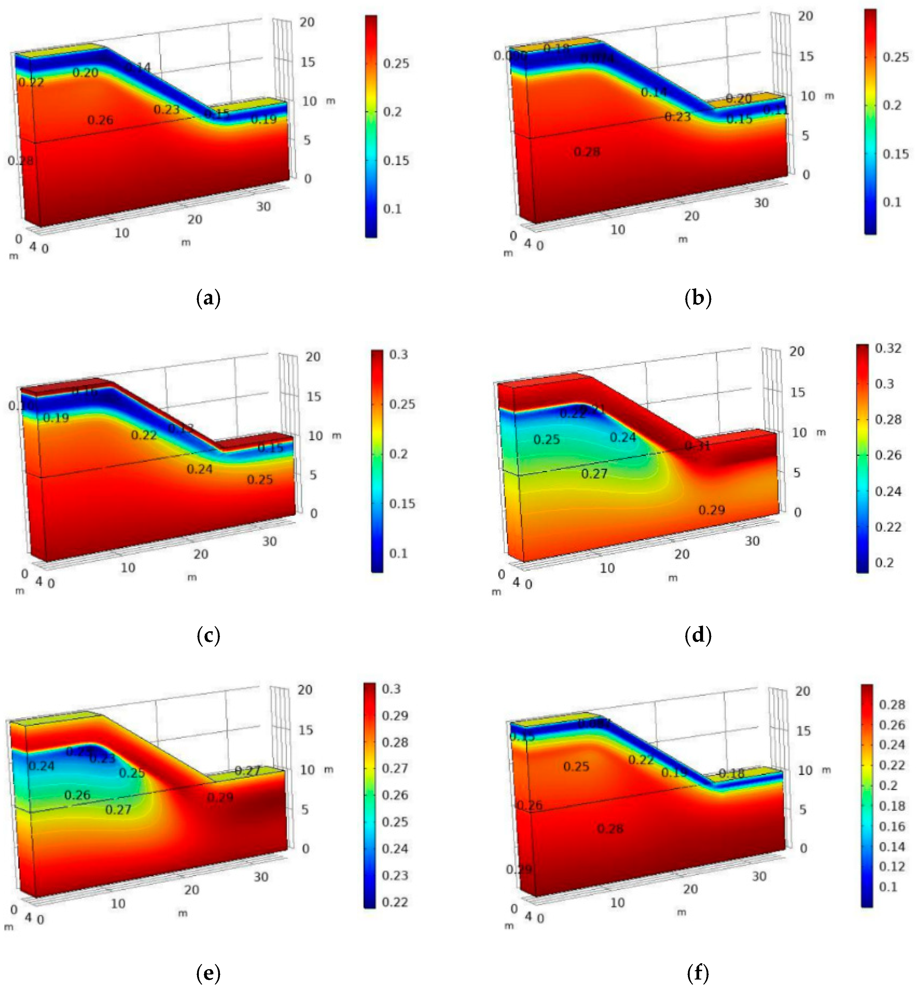
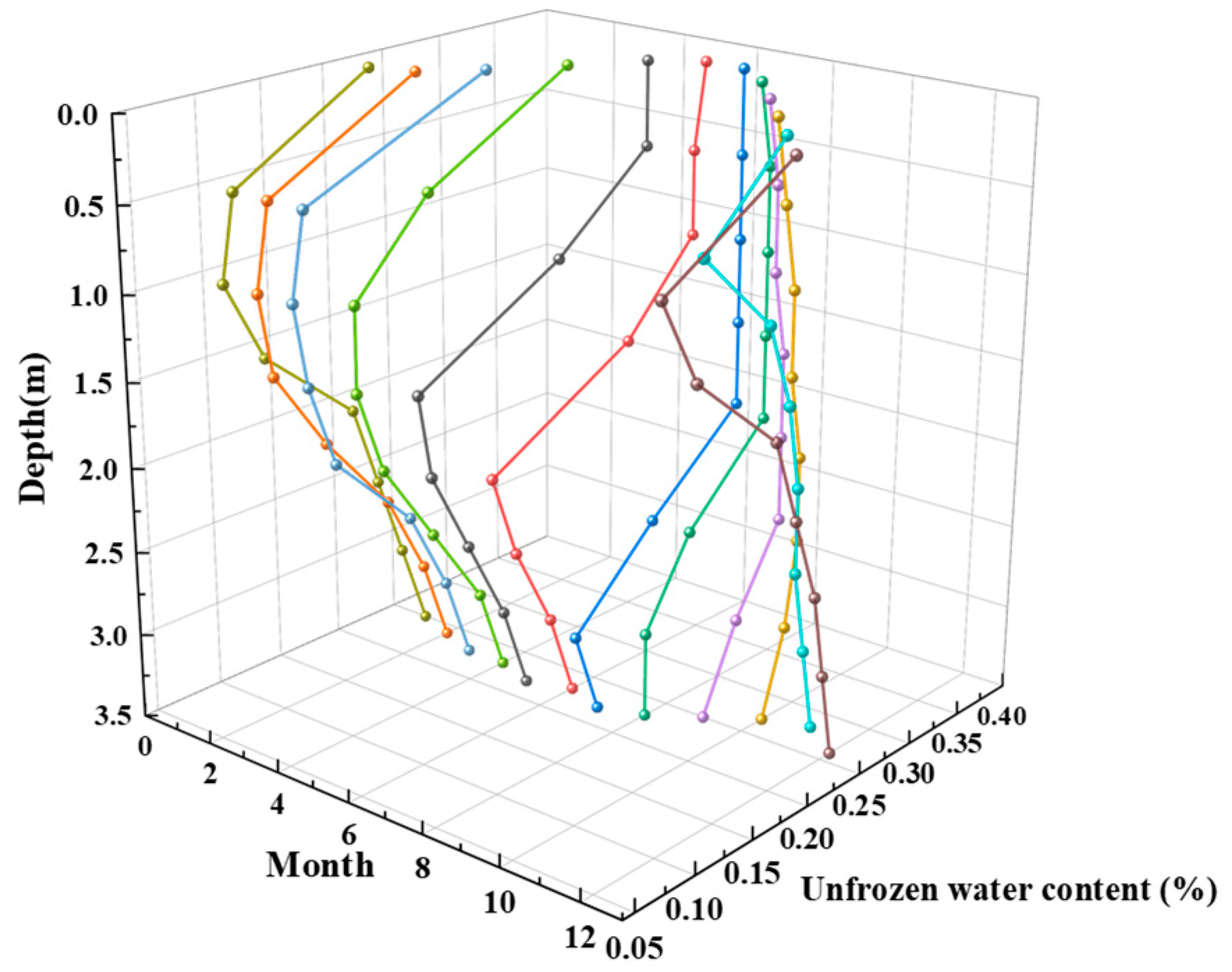
3.2. Moisture Variations under F–T Conditions

Figure 9 shows the distribution of the moisture field of the slope over a year, with the moisture legend on the right side of the figure and the raster scale as the size of the model geometry. Starting from February, the slope surface’s soil moisture content began to gradually increase; water content also gradually increased because in the early stage of soil melting the ambient temperature is low and the slope’s frozen soil melting amount is small and, with the gradual increase in temperature, the soil gradually thaws and the thawing speed is accelerated; the slope surface’s soil moisture accumulation and water content increases rapidly, until it reaches a saturated state of the soil, but because the deep soil is not yet thawed, the frozen soil will prevent the upper layer of the soil from being thawed, and the water content will increase rapidly until the soil becomes saturated. However, because the deep soil has not thawed, frozen soil will stop the upper layer of soil moisture’s downward migration and infiltration; therefore, the upper surface soil moisture content will remain saturated for a period of time or even enter a supersaturated state. Then, with the gradual increase in the external environmental temperature, taking into account the impact of evaporation and water migration, the slope soil’s moisture begins to decline; this stage of the decline in water content is not significant, until the initial freezing period. At the initial stage of the freezing period, the top layer of the soil on the slope starts to freeze, and the water content of the shallow soil starts to decrease faster. Until the end of the freezing period, the water content of the shallow soil is basically unchanged.

Figure 10 shows the variation of unfrozen water content of slope soils as affected by the magnitude of the depth from the slope’s surface over a one-year period, and it can be seen that slope soils are affected by depth to different degrees at different times. From November to December and from January to June, the water content of the slope soil showed a decreasing and then increasing trend with depth, and from July to October, the water content of the slope soil showed an overall decreasing trend with depth. The above phenomenon was analyzed because, in the early stage of soil freezing, the surface layer of the slope body began to freeze, and the water content of the surface layer began to decrease. While the deep soil is not yet frozen and its water content is higher than that of the shallow soil, coupled with the low permeability coefficient of the pulverized clay, the internal migration of water is not strong, the migration of water to the freezing interface is not large, and the water content of the soil under the freezing surface will be reduced. In the thawing period, the shallow frozen soil starts to melt, and the water content starts to increase, but the lower part still has the influence of the frozen layer to prevent the water from migrating downward, resulting in a higher water content for the upper layer of soil, and then an increase in the depth of the water content will reduce first and then increase. After all the shallow soil of the slope body is melted, due to the increasing temperature of the external environment, the water in the surface layer of the slope body is continuously evaporating and being lost. Taking into account the internal migration of water and the existence of the freezing layer, the internal water content of the slope body increases slightly with the increase in depth, and then it decreases again.

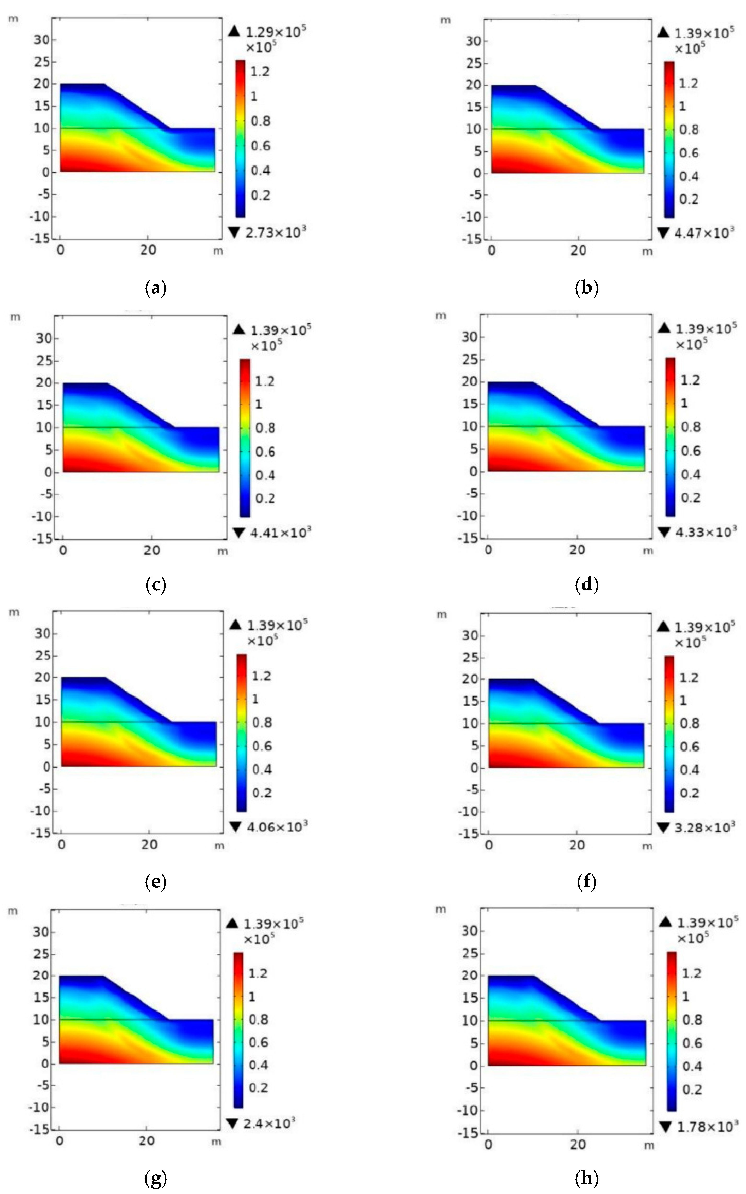
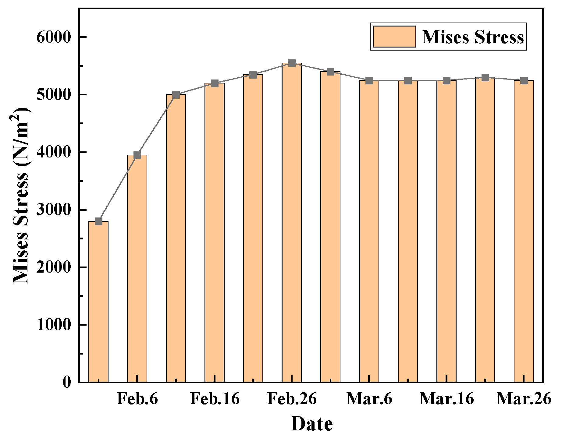
3.3. Stress Variations under F–T Conditions

Analyzing the stability of soil slopes in seasonal permafrost areas not only involves the influence of temperature and moisture, but essentially comes down to the degree of mechanical calculations of the soil material at the end of the day, which should be combined with the dynamic distribution of water and heat inside the slope to calculate and study its stability. In order to better reveal the mechanism of landslides during the thawing of slopes in the seasonally frozen regions, the period from February to March was selected to study the internal stress distribution of slopes in this period, and the Mises stress was also output as an indicator of structural failure, as shown in Figure 11 below. In order to visualize the stress distribution, the view angle of the model is adjusted to the positive section. From the figure, it can be seen that the maximum shear stress inside the slope gradually increases from the beginning of February to the middle of February, and after the middle of February, the maximum shear stress inside the slope remains unchanged, which is because the maximum internal stress is mainly concentrated at the bottom of the slope, and the soil body of the slope begins to thaw gradually during the spring thawing period. The influence on the deep soil body is small, so the stress in this region does not change much. Slope surface stress in the early February to mid-February period gradually increases. In mid-February, after the beginning of a gradual decline in the analysis of the above phenomenon, the slope is in the early stages of the spring thaw period: the shallow frozen soil gradually melts, water migrates to make the soil body gradually produce displacement, stress begins to increase in the soil which melts to a certain extent. For the slope at this time, the downward force exceeds the resistance to the slide force and thus produces a slope under the melting slippery phenomenon; the slope is destabilized, and then the stress begins to gradually decline.

In order to intuitively, clearly, and quantitatively find the change in stress of the surface layer of the slope with time, we select the characteristic point inside the slope at 0.5 m from the slope, extract the specific data of the stress of the point, and then draw a graph. As can be seen in Figure 12, the stress at the characteristic point at the beginning of February is the smallest, and, thereafter, the stress at the point gradually increases. The magnitude of the growth is larger at the stage of the beginning of February to the middle of February, the growth rate gradually slows down at the stage of the middle of February to the end of February, and the stress point starts to decrease at the beginning of March until the middle of March. After that, the stress point gradually increases, with a larger increase in the period from early February to mid-February. The growth rate gradually slows down from mid-February to the end of February, and the stress point begins to decrease at the beginning of March, until it stabilizes at some time in the middle of March. Analysis of the causes of the above phenomenon is that it is due to the slope in February in the melting stage: the slope’s surface layer of frozen soil begins to melt, the surface layer of the soil region experiences moisture accumulation, the shear strength of the soil body reduces, and then the relative migration of the soil body begins to appear, resulting in the concentration of stress. Stress gradually increases in the soil body after complete melting, and the stress reaches a peak, which then, due to the slope collapsing, means the stress begins to gradually reduce until it reaches a stable value.

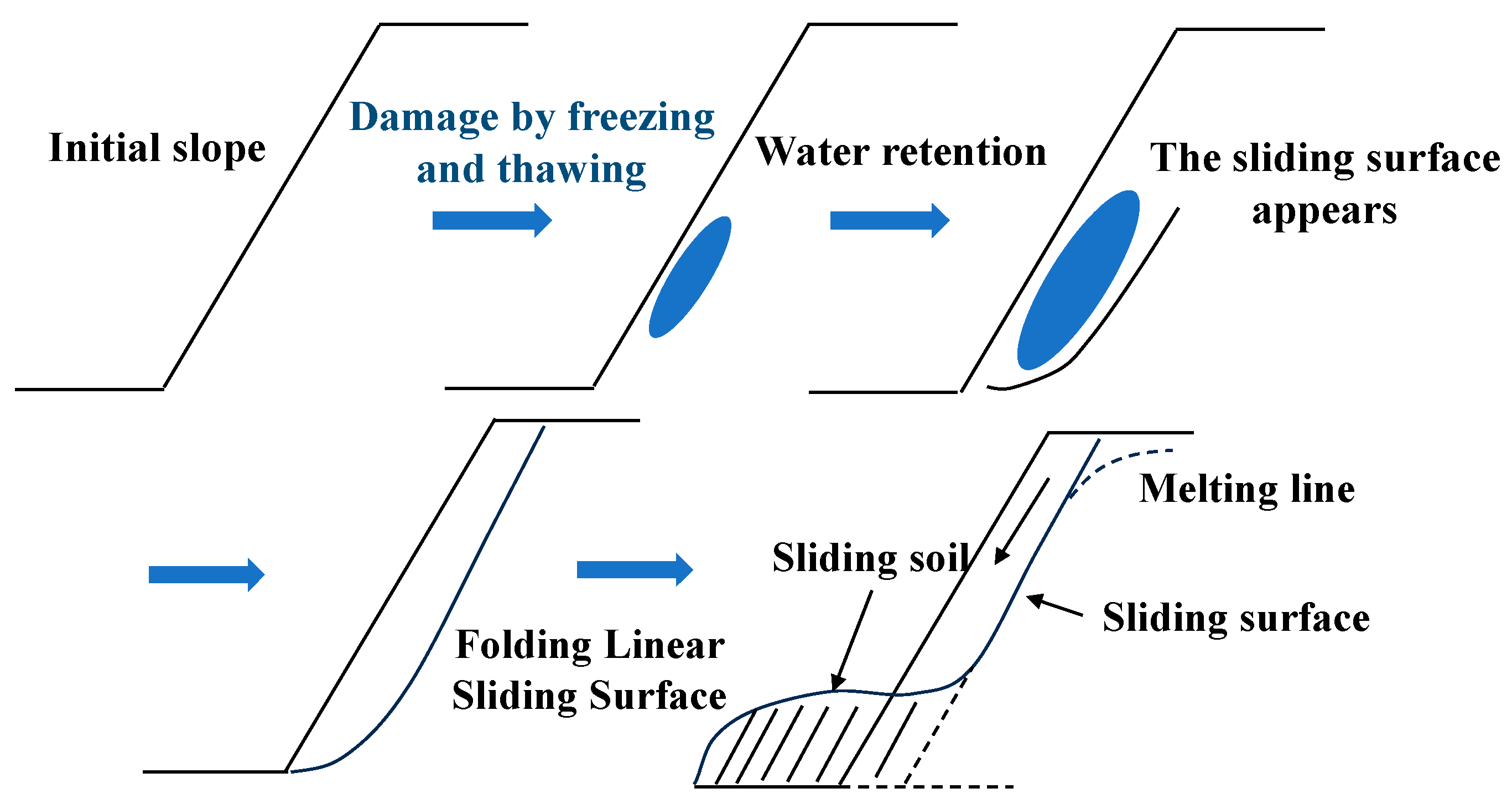
3.4. Analysis of Shallow Melt–Slip Mechanisms on Slopes

According to the results of the above research and analysis, it can be concluded that the landslide of the slope soil body is greatly affected by the F–T effect. In winter, the low temperature of the external environment will make the soil body of the slope produce a certain degree of freezing deformation. As the freezing surface continues to move down, the soil slope’s internal water will migrate to the freezing surface for accumulation, and in the spring thaw period of the slope, there is snow melt and rainfall infiltration and so on, which will make the original slope surface’s soil moisture content gradually increase, until it reaches a state of oversaturation. At this time, the surface layer of the slope will very easily slide and displace. Two main phenomena will occur. First, a number of F–T cycles produced gravity erosion creep of the soil. Due to the cyclic F–T cycle in the spring thawing period, the phase state of the saturated soil also presents cyclic back and forth changes. The soil volume in the process of F–T experiences the rise and fall phenomenon, which makes the soil along the direction of the slope undergo relative displacement, which will lead to the occurrence of structural damage for the slope surface layer and for the soil body. Secondly, the slide bed collapse phenomenon is formed by the continuous downward movement of the freezing depth. In the thawing period of the slope surface’s frozen soil, the outside to the inside gradually begins to melt, and the freezing front gradually moves downward, as does the slope body within the freeze–thaw interface. For the interface above the thawed soil, there is a large amount of moisture accumulation; its shear strength has great attenuation, so the interface at the shallow sliding collapse damage site is multi-layer. Most of the time, most of the sliding surface for the flat straight-line pattern is as shown in Figure 13. Figure 13 shows the dynamic schematic diagram of the slope melt–slip process.

4. Conclusions

To address the engineering geology and highway engineering technical problems of the Suihua–Bei’an Expressway, this paper establishes a three-dimensional slope model with hydrothermal–hydraulic coupling based on COMSOL Multiphysics numerical simulation software in the monsoon frozen zone, and it analyzes and obtains the thawing and sliding mechanism of the slope during the spring thawing period. These findings provide essential knowledge for developing sustainable construction practices that can mitigate the impact of slope thawing and sliding on infrastructure and the environment. The main research results are as follows:

(1)

Suibei Expressway’s slope’s initial freezing period was in the month of October. The initial period of thawing took place the month of February, with the temperature rising. In the thawing stage of the soil body, the F–T of the interface will gradually decrease. In the whole process of the slope soil being subjected to F–T, the external ambient temperature has a greater impact on the shallow soil layer of the slope, and a smaller impact on the deep soil layer.

(2)

In the spring thawing stage, the shallow soil layer of the slope starts to thaw, but the deep soil layer is not yet thawed, due to the low permeability coefficient of the low liquid limit powdery clay which will prevent the upper layer of water from migrating downward, so it will result in the accumulation of water in the shallow layer of the slope, which will lead to the thawing and sliding phenomenon of the slope.

(3)

In the seasonal freezing area of powdery clay road graben slopes, in the spring thaw period after destabilization a sliding surface will form, resulting in the phenomenon of thaw–slip slopes. The sliding surface is not the same as the traditional arc sliding surface because it is a straight-folding-line-type sliding surface. The plastic deformation area of the slope soil is also concentrated in the surface layer of the slope, and the slope melt–slip is actually the processes of the melting and sliding of the shallow slope.

In conclusion, this paper contributes to a deeper understanding of the mechanisms of spring thaw–slip on slopes in seasonally frozen areas and provides implications for the environment and infrastructure. By incorporating these findings into engineering and construction practices, we can effectively contribute to the sustainable development of highways that are resilient to the challenges posed by seasonal freezing zones, thereby contributing to long-term ecological stability and regional socio-economic recovery.

References

1. Zhu, Z.Y.; Ling, X.Z.; Wang, Z.Y.; Lu, Q.R.; Chen, S.J.; Zou, Z.Y.; Guo, Z.H. Experimental investigation of the dynamic behavior of frozen clay from the Beiluhe subgrade along the QTR. Cold Reg. Sci. Technol. 2011, 69, 91–97. [Google Scholar] [CrossRef]
2. Tang, Y.Q.; Zhou, J.; Hong, J.; Yang, P.; Wang, J.X. Quantitative analysis of the microstructure of Shanghai muddy clay before and after freezing. Bull. Eng. Geol. Environ. 2012, 71, 309–316. [Google Scholar] [CrossRef]
3. Ling, X.Z.; Zhang, F.; Li, Q.L.; An, L.S.; Wang, J.H. Dynamic shear modulus and damping ratio of frozen compacted sand subjected to freeze–thaw cycle under multi-stage cyclic loading. Soil Dyn. Earthq. Eng. 2015, 76, 111–121. [Google Scholar] [CrossRef]
4. Lv, Y.; Wang, H.; Gu, C. Study of shear strength of silty clay under freeze-thaw cycle. In Proceedings of the International Conference on Advances in Civil Engineering, Energy Resources and Environment Engineering (ACCESE), Jilin, China, 28–30 June 2019; p. 330. [Google Scholar]
5. Chen, H.; Guo, H.; Yuan, X.; Chen, Y.; Sun, C. Effect of Temperature on the Strength Characteristics of Unsaturated Silty Clay in Seasonal Frozen Region. KSCE J. Civ. Eng. 2020, 24, 2610–2620. [Google Scholar] [CrossRef]
6. Hu, T.; Liu, D.; Wu, H. Experimental Testing and Numerical Modelling of Mechanical Behaviors of Silty Clay under Freezing-Thawing Cycles. Math. Probl. Eng. 2020, 2020, 1–13. [Google Scholar] [CrossRef]
7. Chen, H.; Zhen, D. Quantitative Analysis of the Microstructures of Deep Silty Clay Subjected to Two Freezing–Thawing Cycles under Subway Vibration Loading. J. Cold Reg. Eng. 2021, 35, 452. [Google Scholar]
8. Wenjun, Z.; Qingzhi, W.; Jianhong, F.; Kejin, W.; Xiangqing, Z. Study of the Mechanical and Microscopic Properties of Modified Silty Clay under Freeze-Thaw Cycles. Geofluids 2022, 2022, 3–7. [Google Scholar] [CrossRef]
9. Xu, W.; Wang, X. Effect of Freeze-Thaw Cycles on Mechanical Strength and Microstructure of Silty Clay in the Qinghai-Tibet Plateau. J. Cold Reg. Eng. 2022, 36, 04021018. [Google Scholar] [CrossRef]
10. Song, C.; Qi, J.; Liu, F. Influence of F-T on the mechanical properties of loess in Lanzhou. Geotechnics 2008, 29, 1077–1080. [Google Scholar]
11. Wang, X.; Yang, P.; Wang, H.; Dai, H. Experimental study on effects of freezing and thawing on mechanical properties of clay. J. Geotech. Eng. 2009, 31, 1768–1772. [Google Scholar]
12. Qi, J.; Ma, W. Mechanical properties of permafrost and current research status. Geotechnics 2010, 31, 133–143. [Google Scholar]
13. Chang, D.; Liu, J.; Li, X.; Yu, Q. Experimental study on the effect of freeze-thaw cycle on the mechanical properties of Qinghai-Tibetan silt sandy soil. J. Rock Mech. Eng. 2014, 33, 1496–1502. [Google Scholar]
14. Zheng, Y.; Ma, W.; Bing, H. Experimental study on the effect of freeze-thaw cycle on soil structural properties and analysis of the influence mechanism. Geotechnics 2015, 36, 1282–1287+1294. [Google Scholar]
15. Hu, T.; Liu, J.; Fang, J.; Chang, D.; Liu, D. Experimental study on the effect of cooling temperature on mechanical properties of pulverized clay under freeze-thaw cycle. J. Rock Mech. Eng. 2017, 36, 1757–1767. [Google Scholar]
16. Rogers, N.W.; Selby, M.J. Mechanisms of shallow translational landsliding during summer rainstorms: North Island, New Zealand. Geogr. Ann. Ser. A Phys. Geogr. 1980, 62, 11–21. [Google Scholar] [CrossRef]
17. Lim, T.T.; Rahardjo, H.; Chang, M.F.; Fredlund, D.G. Effect of rainfall on matric suctions in a residual soil slope. Can. Geotech. J. 1996, 33, 618–628. [Google Scholar] [CrossRef]
18. Pasuto, A.; Silvano, S. Rainfall as a trigger of shallow mass movements. A case study in the Dolomites, Italy. Environ. Geol. 1998, 35, 184–189. [Google Scholar] [CrossRef]
19. Eigenbrod, K.D.; Kaluza, D. Shallow slope failures in clays as a result of decreased evapotranspiration subsequent to forest clearing. Can. Geotech. J. 1999, 36, 111–118. [Google Scholar] [CrossRef]
20. Shakoor, A.; Smithmyer, A.J. An analysis of storm-induced landslides in colluvial soils overlying mudrock sequences, southeastern Ohio, USA. Eng. Geol. 2005, 78, 257–274. [Google Scholar] [CrossRef]
21. Gullà, G.; Niceforo, D.; Ferraina, G.; Aceto, I.; Antronico, L. Monitoring station of soil slips in a representative area of Calabria (Italy). In Proceedings of the IX International Symposium on Landslides, Rio De Janeiro, Brazil, 28 June–2 July 2004; Volume 28, pp. 591–596. [Google Scholar]
22. Claessens, L.; Schoorl, J.M.; Veldkamp, A. Modelling the location of shallow landslides and their effects on landscape dynamics in large watersheds: An application for Northern New Zealand. Geomorphology 2007, 87, 16–27. [Google Scholar] [CrossRef]
23. Dahal, R.K.; Hasegawa, S.; Nonomura, A.; Yamanaka, M.; Masuda, T.; Nishino, K. Failure characteristics of rainfall-induced shallow landslides in granitic terrains of Shikoku Island of Japan. Environ. Geol. 2009, 56, 1295–1310. [Google Scholar] [CrossRef]
24. Van Asch TW, J.; Buma, J.; Van Beek, L.P.H. A view on some hydrological triggering systems in landslides. Geomorphology 1999, 30, 25–32. [Google Scholar] [CrossRef]
25. Heilongjiang Cold Land Building Science Research Institute. JGJ 118-2011; Design specification for foundation of building in tundra area; China Construction Industry Press: Beijing, China, 2012. [Google Scholar]
26. Xu, X.; Wang, J.; Zhang, L. Physics of Permafrost; Science Press: Beijing, China, 2001. [Google Scholar]
27. Cui, Y.; Yang, Z.; Shi, W.; Ling, X.; Tu, Z. Experimental study on one-dimensional soil column modeling of unsaturated expansive soil under freeze-thaw cycle. J. Xi’an Univ. Archit. Technol. 2021, 53, 393–403. [Google Scholar]
28. Zhang, Y. Study on the Stability of High-speed Railway Roadbed in Deep Seasonal Freezing Soil Area. Ph.D. Thesis, Beijing Jiaotong University, Beijing, China, 2015; p. 193. [Google Scholar]
29. Lin, B. Research on Mechanical Properties of Freeze-Thaw Clay and Permanent Deformation of Roadbed in Seasonal Freezing Zone; Harbin Institute of Technology: Harbin, China, 2019; p. 214. [Google Scholar]
Figure 1. Geometric model structural dimensions and model meshing.
Sustainability 16 01623 g001
Figure 2. Soil column model.
Sustainability 16 01623 g002
Figure 3. Clouds of soil column temperature and moisture changes with time.
Sustainability 16 01623 g003
Figure 4. Soil column temperature and water content versus depth curve. (a) Temperature; (b) water content.
Sustainability 16 01623 g004
Figure 5. Decadal temperature data for the Sui Bei Region.
Sustainability 16 01623 g005
Figure 6. Model layering and initial geostress equilibrium.
Sustainability 16 01623 g006
Figure 7. Cloud map of temperature field distribution on the slope over one year. (a) 10 January; (b) 10 February; (c) 10 April; (d) 10 September; (e) 10 October; (f) 10 December.
Sustainability 16 01623 g007
Figure 8. Temperature variation curves at different depths.
Sustainability 16 01623 g008
Figure 9. Cloud map of the distribution of unfrozen water content on slopes over the course of a year. (a) 10 January; (b) 10 February; (c) 10 April; (d) 10 September; (e) 10 October; (f) 10 December.
Sustainability 16 01623 g009
Figure 10. Variation curves of unfrozen water content at different depths.
Sustainability 16 01623 g010
Figure 11. Cloud view of Mises stress distribution during spring thaw of the slope. (a) 1 February; (b) 11 February; (c) 16 February; (d) 26 February; (e) 1 March; (f) 11 March; (g) 16 March; (h) 26 March.
Sustainability 16 01623 g011
Figure 12. Mises stress change law of slope surface.
Sustainability 16 01623 g012
Figure 13. Schematic diagram of the slope melt–slip process.
Sustainability 16 01623 g013