Circular Economy Similarities in a Group of Eastern European Countries: Orienting towards Sustainable Development

Abstract

The transition to a circular economy determines benefits at the level of each country by ensuring the premises for a sustainable economy in the future. The purpose of this study is to analyze indicators that measure the results of the implementation of circular economy through five study directions: Production and Consumption, Waste Management, Secondary Raw Materials, Competitiveness and Innovation, and Global Sustainability and Resilience. The analysis used 11 indicators that allow for the measurement of the evolution of eight Eastern European countries in the years 2012–2020. The study used three working hypotheses, which were all verified. The obtained results allowed for the classification of countries using a composite index and the grouping of countries with the help of cluster analysis using Pearson’s correlation coefficient. In a nutshell, sustainable development requires both economic development and environmental sustainability, and the developed composite index groups the countries’ evolution towards this goal.

1. Introduction

One of the main challenges of the 21st century is the sustainable development of countries and the continuous increase in the standard of living of the population, considering certain limitations in the exploitation of resources so that the global ecosystem is not destabilized [1]. Natural resources are considered the key factors in sustainable economic and social development. The extensive consumption of material resources requires sustainable resource management (SRM) to limit resource depletion and control environmental impacts, climate change and biodiversity loss [2,3]. SRM involves the harmonization of economic and environmental objectives, specified in Lenzen’s studies through the convergence between United Nations Sustainable Development Goals (SDG) 12.2 (sustainable management of natural resources) and 8.4 (improving resource efficiency) [4]. Some specialists believe that the scale effect will lead to improved efficiency [5]; others believe that globalization increases the efficient consumption of natural resources through the effects of dematerialization and substitution (reformation of production processes) [6]. Based on these considerations, the concept of the circular economy has gained special attention in global debates, supporting the need to make joint efforts to ensure a better future [7,8,9]. The concept of the circular economy (CE), both for society and for industry, implies the implementation of sustainable development strategies [8] to prevent depletion of resources, to reduce dependence on exploitation, and at the same time to reduce emissions levels [10,11,12].

CE refers to production and consumption operating on the basic principles of reduction, reuse, recycling and recovery of existing materials and products [13,14,15]. Thus, CE can be understood as a regenerative economy that captures resources to be used repeatedly so that waste is minimized and returned to production processes [16,17]. This has a positive impact on the environment [12,18] by minimizing the exploitation and processing of resources [19,20]. Consequently, CE counteracts the harmful effects of the linear economy, which tends to over-exploit resources and produce large amounts of waste [7,19]. The integration of the CE concept implies a systemic change [21] that leads to long-term sustainability, by decoupling economic development from prioritizing the use of natural resources and by the creation of alternative solutions [22,23]. However, despite the benefits of implementing a CE, Blum emphasizes that these practices do not lead to a lower use of resources [23]. Other studies show us that CE contributes to sustainable development [24,25], improves economic processes [26,27], and creates the necessary conditions for innovation [28,29,30].

Sustainable development through the prism of CE is considered by some authors to have a triple result: it contributes to the coordinated development of the economy, of society, and of the environment [31,32]. This also creates the prerequisites for economic performance [32,33].

Some studies emphasize a positive relationship between sustainable development and innovation [34,35,36] as an effect of the circular economy, and others consider the involvement of companies to be vital in this endeavor [37]. Stakeholder theory argues that the circular economy innovation will bring benefits that contribute to economic, social, and environmental performance [38,39]. Through technological development and environmental protection, customer satisfaction increases [23,31] and new products and services are offered, which increases the organization’s competencies and results in greater value to both the organization and society [36,38].

Other studies provide us with information about the beneficial effect of the circular economy through the introduction of digitization through technologies and digital information, which allows for better management of the life cycle, the supply chain, and the adoption of the circular business model (CBM) and product–service systems (PSS) when it comes to machines and equipment [40,41].

The circular economy has gained ground for continued study as an approach to achieving local, national, and global sustainability [42]. Thus, decision-makers in industrialized countries [43], the academic research community [44], and international development practitioners [45,46] have begun to pay attention to CE practices in developing countries to achieve SDG.

Post-industrial recycling (PIR) and post-consumer recycling (PCR) are measures used to sustain resources by improving material circularity and sustainability [47]. At the same time, the study developed by Paulik demonstrates the need to include both circularity and life cycle sustainability indicators when evaluating circularity [48]. Grdic et al., in their study, show us that the application of the circular economy concept can lead to economic growth and GDP growth, ensuring better environmental protection [49]. Cristian Busu and Mihail Busu analyzed circular economy processes through mathematical modeling, and the results show the advantages of using these processes in terms of sustainable economic growth based on the efficient and responsible consumption of resources [50]. Ecologically efficient circularity (EeC) brings up the concept of “eco-efficiency”, which proposes a reduced use of resources generating a greater or equal amount of economic activity [51]. Eco-efficiency is also measured in the analysis and development of sustainability in various studies, and indicates the empirical relationship between the cost of economic activities and the impact on the environment [52,53].

Starting from existing studies [49,50], we see that the benefits of the circular economy and support for sustainable economies can only be obtained by ensuring the reintegration of reusable materials into the circuit, through competitiveness and innovation and through effective measures to adapt to global sustainability and resilience, which the current study wants to measure.

The importance of this study consists in identifying the steps taken by these countries because of the transformations and changes that occurred during nine years (2012–2020) of transition from a linear economy to a circular economy. Thus, the study helps us through examining the values related to the studied indicators during these nine years. The reintroduction of recycled materials into the production and consumption circuit, waste management, and the global effort towards the circular economy help us to classify and group countries from the sustainable perspective so necessary for managerial decision-makers.

The novelty of this study consists in the analysis of eight countries from Eastern Europe by means of a composite index, which groups the countries according to similarities in efforts to improve the efficiency of resources and their sustainable management.

The research aimed to analyze the variability of eight indicators grouped into five study directions, and the countries studied are countries that had similar economic conditions because of political governance. As mentioned above, these ex-communist countries have evolved differently despite having a similar political background, thus proving an important subject of analysis.

The main hypotheses of this study are: (H1) “Is the production and consumption of recycled materials a continuous concern at the level of CE countries?”, (H2) “Does waste management allow for selection and direct contribution to CE?” and (H3) “Does the overall result obtained by each country through the CE indicators allow for the classification and grouping of countries according to common characteristics?”.

The purpose of this study is to test the proposed hypotheses and classify the countries according to the results. To verify the hypotheses, the following analyses were performed: (1) Data analysis for missing values and relative proportions scale, (2) Analysis of the variability of each indicator and the variability among the indicators according to the studied directions, and (3) Analysis of values related to the composite indicator for each country and cluster analysis using Pearson’s correlation.

2. Materials and Methods

In this study, an analysis was carried out based on 11 indicators extracted from the Eurostat database [54] for monitoring circular economies in the period 2012–2020 (see Appendix A—

Table A1. Initial data ShMatFootp.

ShMatFootp	BG	CZ	EE	LT	HU	PL	RO	SK
2012	0.1220	0.1099	0.2066	0.1148	0.0635	0.1320	0.1421	0.1091
2013	0.1254	0.0953	0.2009	0.1349	0.0716	0.1183	0.1380	0.1156
2014	0.1317	0.1124	0.1768	0.1279	0.0898	0.1132	0.1389	0.1093
2015	0.1342	0.1185	0.1746	0.1192	0.0867	0.1145	0.1606	0.0917
2016	0.1247	0.1119	0.1716	0.1283	0.0836	0.1188	0.1652	0.0957
2017	0.1208	0.1117	0.1878	0.1338	0.0891	0.1199	0.1440	0.0930
2018	0.1319	0.1046	0.1886	0.1259	0.0922	0.1185	0.1474	0.0910
2019	0.1324	0.1043	0.1695	0.1273	0.0966	0.1136	0.1719	0.0844
2020	0.1275	0.0962	0.1720	0.1399	0.0910	0.1087	0.1827	0.0819

,

Table A2. Initial data ShResProd.

ShResProd	BG	CZ	EE	LT	HU	PL	RO	SK
2012	0.0560	0.1629	0.0893	0.1454	0.1948	0.0973	0.0672	0.1874
2013	0.0593	0.1700	0.0883	0.1279	0.1778	0.1058	0.0695	0.2014
2014	0.0562	0.1731	0.0985	0.1451	0.1480	0.1139	0.0716	0.1935
2015	0.0506	0.1713	0.1020	0.1451	0.1529	0.1174	0.0607	0.1999
2016	0.0572	0.1721	0.1031	0.1388	0.1579	0.1132	0.0597	0.1981
2017	0.0578	0.1827	0.0933	0.1314	0.1491	0.1141	0.0709	0.2006
2018	0.0581	0.1861	0.0933	0.1396	0.1378	0.1168	0.0701	0.1982
2019	0.0574	0.1818	0.1033	0.1307	0.1330	0.1221	0.0585	0.2133
2020	0.0558	0.1851	0.1015	0.1231	0.1439	0.1242	0.0540	0.2124

,

Table A3. Initial data RecyRateEl.

RecyRateEl	BG	CZ	EE	LT	HU	PL	RO	SK
2012	0.8400	0.8100	0.8000	0.6900	0.8200	0.7600	0.8400	0.8800
2013	0.8400	0.9100	0.6600	0.7000	0.8800	0.7600	0.8700	0.8500
2014	0.8500	0.8600	0.8500	0.7600	0.8700	0.7400	0.8700	0.9100
2015	0.8600	0.8300	0.8700	0.8100	0.8300	0.7000	0.6600	0.8700
2016	0.8200		0.8700	0.8200	0.8400	0.8200	0.7400	0.8900
2017	0.8400	0.8700	0.8600	0.8200	0.8400	0.8300	0.8300	0.8900
2018	0.8100	0.8500	0.8600	0.8200	0.8400	0.8800	0.8300	0.8900
2019	0.8300	0.9300	0.8100	0.8300	0.8400	0.8200	0.8300	0.9100
2020	0.8400	0.8900	0.8200	0.8200	0.8200	0.8600	0.8300	0.9300

,

Table A4. Initial data RecyRatePk.

RecyRatePk	BG	CZ	EE	LT	HU	PL	RO	SK
2012	0.6700	0.7000	0.6100	0.6200	0.4900	0.4100	0.5700	0.6800
2013	0.6600	0.7000	0.5800	0.5400	0.4900	0.3600	0.5300	0.6600
2014	0.6200	0.7300	0.6000	0.5800	0.4800	0.5500	0.5500	0.6500
2015	0.6400	0.7400	0.5900	0.6000	0.5000	0.5800	0.5600	0.6400
2016	0.6400	0.7500	0.5600	0.7000	0.5000	0.5800	0.6000	0.6600
2017	0.6600	0.7200	0.5400	0.6200	0.5000	0.5700	0.6000	0.6600
2018	0.6000	0.7000	0.6000	0.6100	0.4600	0.5900	0.5800	0.6700
2019	0.6100	0.7100	0.6600	0.6200	0.4700	0.5600	0.4500	0.6800
2020		0.6800	0.7100	0.6200	0.5200		0.4000	0.7100

,

Table A5. Initial data RecyRateMn.

RecyRateMn	BG	CZ	EE	LT	HU	PL	RO	SK
2012	0.2500	0.2300	0.1900	0.2400	0.2600	0.1200	0.1500	0.1300
2013	0.2900	0.2400	0.1800	0.2800	0.2600	0.1500	0.1300	0.1100
2014	0.2300	0.2500	0.3100	0.3100	0.3100	0.2700	0.1300	0.1000
2015	0.2900	0.3000	0.2800	0.3300	0.3200	0.3300	0.1300	0.1500
2016	0.3200	0.3400	0.2800	0.4800	0.3500	0.3500	0.1300	0.2300
2017	0.3500	0.3200	0.2800	0.4800	0.3500	0.3400	0.1400	0.3000
2018	0.3200	0.3200	0.2800	0.5300	0.3700	0.3400	0.1100	0.3600
2019	0.3500	0.3300	0.3100	0.5000	0.3600	0.3400	0.1200	0.3900
2020	0.3500	0.4100	0.2900	0.4500	0.3200	0.3900	0.1200	0.4500

,

Table A6. Initial data CMatUseR.

CMatUseR	BG	CZ	EE	LT	HU	PL	RO	SK
2012	0.0200	0.0600	0.1900	0.0400	0.0600	0.1100	0.0300	0.0400
2013	0.0300	0.0700	0.1500	0.0300	0.0600	0.1200	0.0300	0.0500
2014	0.0300	0.0700	0.1100	0.0400	0.0500	0.1300	0.0200	0.0500
2015	0.0300	0.0700	0.1100	0.0400	0.0600	0.1200	0.0200	0.0500
2016	0.0400	0.0800	0.1200	0.0500	0.0700	0.1000	0.0200	0.0500
2017	0.0400	0.0900	0.1200	0.0500	0.0700	0.1000	0.0200	0.0500
2018	0.0300	0.1100	0.1400	0.0400	0.0700	0.1000	0.0200	0.0500
2019	0.0200	0.1100	0.1600	0.0400	0.0700	0.1000	0.0100	0.0600
2020	0.0600	0.1200	0.1600	0.0400	0.0500	0.0800	0.0200	0.0100

,

Table A7. Initial data ShTradeRwM.

ShTradeRwM	BG	CZ	EE	LT	HU	PL	RO	SK
2012	0.1000	0.0200	0.1200	0.2600	0.0400	0.2300	0.2200	0.0200
2013	0.1000	0.0200	0.1500	0.2600	0.0300	0.2100	0.2000	0.0300
2014	0.0900	0.0200	0.1400	0.2700	0.0300	0.2400	0.1800	0.0200
2015	0.1000	0.0200	0.0800	0.2800	0.0300	0.2500	0.2100	0.0300
2016	0.1100	0.0200	0.0900	0.2600	0.0400	0.2800	0.1500	0.0400
2017	0.1200	0.0200	0.0800	0.2400	0.0400	0.2400	0.2000	0.0600
2018	0.1000	0.0200	0.0800	0.2600	0.0300	0.2300	0.2300	0.0500
2019	0.0900	0.0100	0.0800	0.2700	0.0600	0.2300	0.2300	0.0300
2020	0.1000	0.0200	0.0800	0.2400	0.0600	0.2500	0.2200	0.0200

,

Table A8. Initial data ShPrivInvest.

ShPrivInvest	BG	CZ	EE	LT	HU	PL	RO	SK
2012	0.0755	0.0699	0.3324	0.0824	0.0770	0.0857	0.1451	0.1319
2013	0.0670	0.0817	0.2719	0.0952	0.0885	0.0941	0.1491	0.1525
2014	0.0808	0.0663	0.1465	0.1027	0.1156	0.0980	0.2514	0.1387
2015	0.1019	0.0798	0.1595	0.1014	0.1236	0.1100	0.1725	0.1512
2016	0.0896	0.0744	0.1704	0.1481	0.1198	0.0869	0.1575	0.1534
2017	0.0917	0.0787	0.1657	0.1736	0.1160	0.0889	0.1579	0.1275
2018	0.0960	0.0856	0.1800	0.1209	0.1204	0.1287	0.1357	0.1327
2019	0.0984	0.0880	0.1773	0.1171	0.1275	0.1261	0.1547	0.1110
2020	0.0935	0.0881	0.1770	0.1381	0.1228	0.1085	0.1523	0.1197
2021	0.0936	0.0901	0.1753	0.1418	0.1228	0.1093	0.1480	0.1192

,

Table A9. Initial data ShGrAddVal.

ShGrAddVal	BG	CZ	EE	LT	HU	PL	RO	SK
2012	0.0700	0.1200	0.2100	0.0900	0.1300	0.1200	0.1100	0.1600
2013	0.0700	0.1200	0.2100	0.0900	0.1300	0.1200	0.1100	0.1500
2014	0.0800	0.1200	0.2100	0.1000	0.1300	0.1300	0.1200	0.1100
2015	0.0900	0.1300	0.2000	0.1000	0.1200	0.1200	0.1200	0.1200
2016	0.0800	0.1200	0.2000	0.1200	0.1200	0.1100	0.1200	0.1200
2017	0.0900	0.1200	0.2000	0.1200	0.1300	0.1100	0.1300	0.1100
2018	0.0800	0.1200	0.1900	0.1200	0.1400	0.1100	0.1300	0.1100
2019	0.0900	0.1200	0.1900	0.1200	0.1200	0.1100	0.1300	0.1200
2020	0.0900	0.1200	0.2000	0.1200	0.1200	0.1100	0.1300	0.1100

,

Table A10. Initial data MatImpDep.

MatImportDep	BG	CZ	EE	LT	HU	PL	RO	SK
2012	0.1520	0.2990	0.2080	0.4180	0.3170	0.1640	0.0970	0.4420
2013	0.1570	0.3180	0.1950	0.3860	0.3050	0.1610	0.0920	0.4580
2014	0.1450	0.3180	0.2040	0.3990	0.2770	0.1720	0.0930	0.4200
2015	0.1410	0.3300	0.1870	0.4070	0.2700	0.1780	0.0920	0.4240
2016	0.1610	0.3230	0.2250	0.4040	0.2830	0.1790	0.0990	0.4250
2017	0.1680	0.3310	0.2100	0.3920	0.2980	0.1830	0.1070	0.4290
2018	0.1570	0.3300	0.2370	0.4140	0.2970	0.1940	0.1060	0.4300
2019	0.1640	0.3300	0.2410	0.4050	0.2730	0.1940	0.0950	0.4400
2020	0.1600	0.3140	0.2640	0.3670	0.2620	0.1970	0.0910	0.4280

and

Table A11. Initial data ShGasEmiss.

ShGasEmiss	BG	CZ	EE	LT	HU	PL	RO	SK
2012	0.1170	0.1572	0.2254	0.0957	0.0761	0.1404	0.0871	0.1011
2013	0.1087	0.1526	0.2549	0.0922	0.0753	0.1414	0.0782	0.0966
2014	0.1179	0.1532	0.2431	0.0979	0.0775	0.1394	0.0785	0.0925
2015	0.1283	0.1557	0.2071	0.1049	0.0829	0.1434	0.0801	0.0974
2016	0.1217	0.1549	0.2212	0.1024	0.0813	0.1439	0.0777	0.0970
2017	0.1229	0.1461	0.2285	0.1047	0.0816	0.1437	0.0771	0.0954
2018	0.1162	0.1484	0.2193	0.1103	0.0834	0.1455	0.0798	0.0971
2019	0.1243	0.1535	0.1706	0.1235	0.0894	0.1534	0.0853	0.1000
2020	0.1200	0.1503	0.1444	0.1445	0.0921	0.1604	0.0890	0.0993

). The information was collected from 8 Eastern European countries: Bulgaria, Czech Republic, Estonia, Lithuania, Hungary, Poland, Romania, and Slovakia, which were indexed as shown in

Table 1. The country indexes.

Index j	Abbrev. Countries	Name of Countries
1	BG	Bulgaria
2	CZ	Czech Republic
3	EE	Estonia
4	LT	Lithuania
5	HU	Hungary
6	PL	Poland
7	RO	Romania
8	SK	Slovakia

.

Table 2. Indicators for circular economy, adapted from Eurostat database [54].

No.	Abbrv.	Directions	MU	Meaning Indicators
1	ShMatFootp	PC	%	world demand for extractive materials (biomass, metal ores, non-metallic minerals, and fossil energy materials/carriers), driven by consumption and investment by households, governments, and businesses in EU countries
2	ShResProd	PC	%	the total amount of materials used directly by an economy
3	RecyRateEl	WM	%	share of electrical and electronic equipment waste
4	RecyRatePk	WM	%	share of recycled plastic packaging waste
5	RecyRateMn	WM	%	share of municipal waste recycled (material recycling, composting and anaerobic digestion)
6	CMatUseR	SRM	%	share of recycled and reintroduced material in the economy, indicating that more secondary materials are replacing primary raw materials, thereby reducing the environmental impact of primary material extraction
7	ShTradeRwM	SRM	%	share of quantities of selected waste categories and by-products that are shipped between EU Member States (intra-EU) and across EU borders (extra-EU)
8	ShPrivInvest	CI	%	share of gross investment in tangible goods in three sectors (recycling, repair and reuse, and the rental and leasing sector). Gross investment in new and existing tangible goods, whether purchased from others or produced for own use (i.e., capitalized production of tangible capital goods), with a useful life of more than one year, including unproduced tangible goods such as the potential value of lands
9	ShGrAddVal	CI	%	includes the share of gross income from operating activities after adjusting for operating subsidies and indirect taxes
10	MatImpDep	GSR	%	the ratio between imports (IMP) and direct material inputs (DMI) in percentage
11	ShGasEmiss	GSR	%	shows the greenhouse gas emissions of all production activities undertaken in the EU economy. This indicator includes emissions from international air transport by EU-resident airlines and excludes emissions from private households

MU—measuring unit, ShMatFootp—Share of material footprint, ShResProd—Share of resource productivity, RecyRateEl—Recycling rate of waste from electrical and electronic equipment, RecyRatePk—Recycling rate of packaging waste, RecyRateMn—Recycling rate of municipal waste, CMatUseR—Circular material use rate, ShTradeRwM—Share of trade in recyclable raw materials per persons employed, ShPrivInvest—Share of private investment per persons employed in circular economy sectors, ShGrAddVal—Share of private investment per persons employed in circular economy sectors, MatImpDep—Material import dependency, ShGasEmiss—Greenhouse gas emissions from production activities, PC—Production and Consumption, WM—Waste management, SRM—Secondary raw materials, CI—Competitiveness and Innovation, GSR—Global sustainability and resilience.

shows the indicators tracking 5 directions: (I) “Production and Consumption”, (II) “Waste management”, (III) “Secondary raw materials”, (IV) “Competitiveness and Innovation”, and (V) “Global sustainability and resilience”.

By analyzing the values related to the indicators studied, this study allows us to identify the steps taken by countries because of the transformations and changes that took place over nine years (2012–2020) of transition from a linear economy to a circular economy. The reintroduction of recycled materials into the production and consumption cycle (tested by hypothesis H1), waste management (tested by hypothesis H2) and the global effort towards the circular economy (tested by hypothesis H3) help us to classify and group countries from a much-needed sustainable perspective for managerial decision-makers. Data analysis and processing involved the completion of three stages: (1) Data analysis for missing values and scale of relative proportions, (2) Analysis of the variability of each indicator and the variability among the indicators according to the studied directions, and (3) Analysis of values related to the composite indicator for each country and cluster analysis using Pearson’s correlation.

2.1. Data Analysis—Missing Values

In some countries in certain years, there were missing data in the Eurostat database for certain indicators, and these had to be filled in according to their own procedures. An example is the entry for CZ in 2016 in RecyRateEl in

Table 3. RecyRateEl observed percentages (O_i,j values) and sums (r = 8, c = 8).

Year	BG	CZ	EE	LT	HU	PL	RO	SK	Sum
2012	84.00	81.00	80.00	69.00	82.00	76.00	84.00	88.00	644.0
2013	84.00	91.00	66.00	70.00	88.00	76.00	87.00	85.00	647.0
2014	85.00	86.00	85.00	76.00	87.00	74.00	87.00	91.00	671.0
2015	86.00	83.00	87.00	81.00	83.00	70.00	66.00	87.00	643.0
2017	84.00	87.00	86.00	82.00	84.00	83.00	83.00	89.00	678.0
2018	81.00	85.00	86.00	82.00	84.00	88.00	83.00	89.00	678.0
2019	83.00	93.00	81.00	83.00	84.00	82.00	83.00	91.00	680.0
2020	84.00	89.00	82.00	82.00	82.00	86.00	83.00	93.00	681.0
Sum	671.0	695.0	653.0	625.0	674.0	635.0	656.0	713.0	5322

and

Table 4. RecyRateEl expected percentages (Ei,j values).

Year	BG	CZ	EE	LT	HU	PL	RO	SK
2012	81.20	84.10	79.02	75.63	81.56	76.84	79.38	86.28
2013	81.57	84.49	79.39	75.98	81.94	77.20	79.75	86.68
2014	84.60	87.63	82.33	78.80	84.98	80.06	82.71	89.90
2015	81.07	83.97	78.89	75.51	81.43	76.72	79.26	86.14
2017	85.48	88.54	83.19	79.62	85.86	80.90	83.57	90.83
2018	85.48	88.54	83.19	79.62	85.86	80.90	83.57	90.83
2019	85.73	88.80	83.43	79.86	86.12	81.13	83.82	91.10
2020	85.86	88.93	83.56	79.97	86.24	81.25	83.94	91.24

. To analyze the full data, a replacement formula for missing values was considered.

The considered parameter Recycling rate of waste of electrical and electronic equipment, collected separately in the instances of missing data in RecyRateEl (see Appendix A—Table A3), depends on the tabulated factors (country and year), and other factors may of course be involved. However, the rest of the factors belong in the category of unanticipated random factors. A multiplicative effects formula may be suitable for estimation of the factor value [55]. Such a multiplicative effects formula recognizes that the value of an entry is influenced by the values of the factors in a natural way. For instance, the demographics of the population evolve with each year; technological development evolves by the year; fiscal conditions and legislation depend on the country.

For such an arrangement, the chi-squared value X² is calculated according to Equation (1) [55]:

$$X^2={\displaystyle \sum _{i=1}^r{\displaystyle \sum _{j=1}^c\frac{{(O_{i,j}-E_{i,j})}^2}{E_{i,j}}}}$$

(1)

where X² is a test that measures how a model compares to actual observed data, O_i,j are the observed frequency values and E_i,j is the expected value calculated for r rows and c columns.

With the assumption of multiplicative effects, E_i,j is calculated according to Equation (2) [55]:

$$E_{i,j}=\left({\displaystyle \sum _{k=1}^r{O}_{i,k}}\right)\left({\displaystyle \sum _{k=1}^c{O}_{k,j}}\right)/\left({\displaystyle \sum _{i=1}^r{\displaystyle \sum _{j=1}^c{O}_{i,j}}}\right)$$

(2)

It is required that some assumptions are met. For instance, formulas should be applied to raw values, not to percentages. If the formulas are applied to percentages, then the significance from the chi-square test may be limited to the standard sample size of a percentage calculation (100).

Consider the case of “RecyRateEl” in Table 3 and Table 4, where the values are in percentages.

${\displaystyle \sum _{i=1}^8{\displaystyle \sum _{j=1}^8{X}_{i,j}^2}}$ = 13.7 from

Table 5. RecyRateEl calculated chi-squares (Xi,j values) and grand total.

Year	BG	CZ	EE	LT	HU	PL	RO	SK	Sum
2012	0.10	0.11	0.01	0.58	0.00	0.01	0.27	0.03	1.12
2013	0.07	0.50	2.26	0.47	0.45	0.02	0.66	0.03	4.46
2014	0.00	0.03	0.09	0.10	0.05	0.46	0.22	0.01	0.96
2015	0.30	0.01	0.83	0.40	0.03	0.59	2.22	0.01	4.39
2017	0.03	0.03	0.09	0.07	0.04	0.05	0.00	0.04	0.35
2018	0.24	0.14	0.09	0.07	0.04	0.62	0.00	0.04	1.25
2019	0.09	0.20	0.07	0.12	0.05	0.01	0.01	0.00	0.55
2020	0.04	0.00	0.03	0.05	0.21	0.28	0.01	0.03	0.65
Sum	0.86	1.02	3.48	1.87	0.87	2.04	3.39	0.20	13.7

, following a chi-square distribution with (8 − 1) × (8 − 1) = 49 degrees of freedom. The probability of the chi-square distribution to observe better agreement is 1.5 × 10⁻⁷, so the hypothesis that the RecyRateEl entries in the Table are actually observations from a multiplicative effect experiment (E_i,j being their expectations) cannot be rejected. Thus, the formula for E_i,j is suitable for making estimations for the missing values, and it was used as such. The estimation was made through program calculations [56] and provided as source code [57] when the estimation minimized X² disagreement.

2.2. Data Analysis—Relative Proportions Scale

For each table, the data have been transformed into a relative scale. Considering O_i,j for 1 ≤ i ≤ r and 1 ≤ j ≤ c, where i are indices for years (from 2012 to 2020) and j are indices for countries (from BG to SK, see Table 1), the new values (to be called ratios, R_i,j) are obtained using Equation (3):

$$R_{i,j}=\frac{O_{i,j}}{{\displaystyle \sum _{k=1}^c{O}_{i,j}}}$$

(3)

as in the initial data (see Appendix A—Table A3) to the processed data of relative ratios for RecyRateEl (see Appendix A—

Table A12. Estimate_RecyRateEl.

RecyRateEl	BG	CZ	EE	LT	HU	PL	RO	SK
2012	80.996	84.136	79.755	76.113	81.531	77.194	78.701	86.228
2013	81.6	84.763	80.349	76.681	82.139	77.77	79.288	86.871
2014	84.375	87.646	83.082	79.289	84.933	80.415	81.985	89.825
2015	81.042	84.184	79.801	76.157	81.578	77.239	78.746	86.278
2016	83.894	87.147	82.609	78.837	84.449	79.957	81.517	89.314
2017	85.201	88.504	83.896	80.065	85.764	81.203	82.787	90.705
2018	85.253	88.559	83.947	80.114	85.817	81.252	82.838	90.761
2019	85.47	88.784	84.16	80.318	86.035	81.459	83.049	90.991
2020	85.6	88.919	84.288	80.44	86.166	81.583	83.175	91.13

). As with the RecyRateEl indicator, estimation calculations were made for the RecyRatePk indicator, where in 2020 there were no data for BG and PL (see Appendix A—Table A4—initial data and

Table A13. Estimate_RecyRatePk.

RecyRatePk	BG	CZ	EE	LT	HU	PL	RO	SK
2012	63.373	70.881	60.273	60.777	48.626	52.638	53.699	66.271
2013	60.458	67.619	57.499	57.981	46.389	50.216	51.228	63.222
2014	63.328	70.830	60.229	60.733	48.591	52.600	53.660	66.223
2015	64.551	72.197	61.392	61.906	49.529	53.616	54.696	67.502
2016	66.501	74.379	63.247	63.777	51.026	55.236	56.349	69.542
2017	64.876	72.561	61.702	62.218	49.779	53.886	54.972	67.843
2018	64.060	71.648	60.926	61.435	49.153	53.208	54.281	66.989
2019	63.460	70.978	60.355	60.860	48.693	52.710	53.773	66.362
2020	64.511	72.153	61.355	61.868	49.499	53.583	54.663	67.461

—processed data).

2.3. Analysis of the Variability of Each Indicator and the Variability among the Indicators According to the Studied Directions

To establish the variability of each indicator, the average of the values of the years studied was calculated according to Equation (4):

$${Aver}_{k,j}=\frac{\sum _{i=1}^8{Y}_{k,i,j}}{8}$$

(4)

where Aver_k,j are the average values of the previous years (2012–2019) corresponding to each indicator in each country, Y_k,i,j is the value of indicator k related to each year i and country j; k—the index assigned to each indicator (see

Table 6. The composite index.

Index k	Indicator Y	Identified Effect
1	ShMatFootp	Positive
2	ShResProd	Positive
3	RecyRateEl	Positive
4	RecyRatePk	Positive
5	RecyRateMn	Positive
6	CMatUseR	Positive
7	ShTradeRwM	Positive
8	ShPrivInvest	Positive
9	ShGrAddVal	Positive
10	MatImpDep	Negative
11	ShGasEmiss	Negative

), k = 1 ÷ 11 (see Table A1, Table A2, Table A3, Table A4, Table A5, Table A6, Table A7, Table A8, Table A9, Table A10 and Table A11), i—the index assigned to each year, i = 2012 ÷ 2019 and j—the index assigned to each country, j = 1 ÷ 8 (see Table 1).

Afterwards, the difference between the value for 2020 and the recorded average was calculated for each country at the level of each indicator according to Equation (5):

$${Diff}_{k,j}=Y_{k,2020,j}-{Aver}_{k,j}$$

(5)

where Y_k,2020,j represents the value of indicator Y with index k (see Table 6) from the year 2020 and from country j (see Table 1)

To determine if the value obtained by “Diff” is statistically significant, Student’s t-test was used. This is a statistical hypothesis test in which the test statistic follows a t distribution of Student’s test using the null hypothesis according to Equation (6).

$$t=\frac{Z}{s}=\frac{\overline{X}-\mu }{\widehat{\sigma }/\sqrt{n}}$$

(6)

In testing the null hypothesis that the population mean is equal to a specified value µ₀, one uses a statistic calculated according to Equation (7).

$$t=\frac{\overline{x}-{\mu }_0}{s/\sqrt{n}}$$

(7)

where $\overline{x}$ is the sample mean, s is the sample standard deviation and n is the sample size. The degrees of freedom used in this test are n − 1.

Within the study directions, the calculations were carried out based on the values obtained from related indicators. To obtain the value related to direction 1 “Production and Consumption”, the values of indicators ShMatFootp and ShResProd were added up, which shows us the results obtained for each country according to Equation (8).

$${PC=Dir}_{1,j}=\sum _{k=1}^2{Y}_{k,2020,j}$$

(8)

where Dir_1,j represents the 1st study direction called PC (Production and Consumption) from country j (see Table 1).

For direction 2 “Waste management” we used the summation of the values of indicators RecyRateEl, RecyRatePk and RecyRateMn, which shows us the results obtained for waste recycling collected by type of waste according to Equation (9).

$${WM=Dir}_{2,j}=\sum _{k=3}^5{Y}_{k,2020,j}$$

(9)

where Dir_2,j represents the 2nd study direction called WM (Waste management) from country j (see Table 1).

For direction 3 “Secondary raw materials” we used the summation of the values of indicators CMatUseR and ShTradeRwM, which shows us the results obtained for secondary materials reintroduced into the economy according to Equation (10).

$${SRM=Dir}_{3,j}=\sum _{k=6}^7{Y}_{k,2020,j}$$

(10)

where Dir_3,j represents the 3rd study direction called SRM (Secondary raw materials) from country j (see Table 1).

For direction 4 “Competitiveness and Innovation” we used the summation of the values of indicators ShTradeRwM and ShPrivInvest, which shows us the results obtained for gross investments in tangible goods and gross income from exploitation activity, according to Equation (11).

$${CI=Dir}_{4,j}=\sum _{k=8}^9{Y}_{k,2020,j}$$

(11)

where Dir_4,j represents the 4th study direction called CI (Competitiveness and Innovation) from country j (see Table 1).

For direction 5 “Global sustainability and resilience” (GSR) we used the summation of the values of indicators MatImpDep and ShGasEmiss, which shows us the results obtained for the ratio between imports and inputs of direct materials on the one hand and greenhouse gas emissions from production activities on the other, according to Equation (12).

$${GSR=Dir}_{5,j}=\sum _{k=10}^{11}{Y}_{k,2020,j}$$

(12)

where Dir_5,j represents the 5th study direction called GSR (Global sustainability and resilience) from country j (see Table 1).

2.4. Analysis of Values Related to the Composite Indicator for Each Country

To obtain a composite index, the desired effect of each indicator was analyzed, assigning it a “positive” effect when an increase in the recorded value was desired and a “negative” effect when a decrease in the recorded value was desired, according to Table 6.

The composite index is calculated as follows (Table 6) according to Equation (13):

$${CI}_{i,j}=\sum _{k=1}^9{Y}_{k,i,j}-\sum _{k=10}^{11}{Y}_{k,i,j}$$

(13)

where CI_i,j is the corresponding composite index.

Subsequently, statistical analysis was performed with a cluster-based multivariate exploratory technique using Statistica software (v. 8.0). Cluster analysis was chosen by means of a unique link (nearest neighbor), thus calculating the distance between two clusters. According to the agglomerative hierarchical algorithm, the distance between the items was calculated; the pair of items that was closest was selected and merged into one class, and then the distance to the other item was calculated. Item classes were recomputed and then repeated until grouping was finally achieved. The distance measurement method was used to find the distance between items through the 1-Pearson-r correlation coefficient.

3. Results and Discussion

3.1. Data Analysis for Missing Values and Relative Proportions Scale

Table RecyRateEl: The 2016 line was added (see Appendix A—Table A12. Estimate_RecyRateEl), and the missing value was obtained (87.147 for CZ and 2016 in RecyRateEl when X² was 15.0009).

RecyRatePk: The 2020 line was added (see Appendix A—Table A13. Estimate_RecyRatePk), and the missing values were obtained (64.511 for BG and 2020, 53.583 for PL and 2020 in RecyRatePk when X² was 23.0395).

3.2. Analysis of the Variability of Each Indicator and the Variability among the Indicators According to the Studied Directions

Table 7. Analysis of the variability of the indicators.

No.	Indicators Year/ Country		BG	CZ	EE	LT	HU	PL	RO	SK
1	ShMatFootp	2020	0.1275	0.0962	0.1720	0.1399	0.0910	0.1087	0.1827	0.0819
		Aver	0.1279	0.1086	0.1846	0.1265	0.0841	0.1186	0.1510	0.0987
		Stdev	0.0052	0.0070	0.0138	0.0068	0.0111	0.0060	0.0130	0.0111
		Diff.	−0.0003	−0.0123	−0.0126	0.0134	0.0068	−0.0099	0.0317	−0.0168
		p_t	0.49	0.28	0.38	0.25	0.42	0.29	0.21	0.30
2	ShResProd	2020	0.0558	0.1851	0.1015	0.1231	0.1439	0.1242	0.0540	0.2124
		Aver	0.0566	0.1750	0.0964	0.1380	0.1564	0.1126	0.0660	0.1991
		Stdev	0.0026	0.0078	0.0061	0.0072	0.0206	0.0077	0.0055	0.0074
		Diff.	−0.0007	0.0101	0.0052	−0.0149	−0.0125	0.0117	−0.0121	0.0133
		p_t	0.46	0.33	0.39	0.24	0.42	0.30	0.23	0.27
3	RecyRateEl	2020	0.1233	0.1307	0.1204	0.1204	0.1204	0.1263	0.1219	0.1366
		Aver	0.1261	0.1306	0.1239	0.1177	0.1274	0.1188	0.1219	0.1336
		Stdev	0.0049	0.0054	0.0100	0.0071	0.0042	0.0068	0.0106	0.0021
		Diff.	−0.0028	0.0001	−0.0035	0.0027	−0.0070	0.0075	0.0000	0.0030
		p_t	0.42	0.50	0.45	0.45	0.29	0.36	0.50	0.32
4	RecyRatePk	2020	0.1338	0.1411	0.1473	0.1286	0.1079	0.1111	0.0830	0.1473
		Aver	0.1332	0.1501	0.1239	0.1275	0.1016	0.1093	0.1159	0.1385
		Stdev	0.0072	0.0032	0.0091	0.0065	0.0038	0.0165	0.0090	0.0052
		Diff.	0.0006	−0.0091	0.0234	0.0011	0.0063	0.0018	−0.0329	0.0088
		p_t	0.49	0.18	0.20	0.48	0.29	0.49	0.12	0.29
5	RecyRateMn	2020	0.1259	0.1475	0.1043	0.1619	0.1151	0.1403	0.0432	0.1619
		Aver	0.1387	0.1338	0.1210	0.1761	0.1486	0.1242	0.0622	0.0955
		Stdev	0.0196	0.0103	0.0185	0.0184	0.0124	0.0267	0.0182	0.0339
		Diff.	−0.0128	0.0137	−0.0167	−0.0142	−0.0335	0.0161	−0.0190	0.0664
		p_t	0.41	0.33	0.38	0.40	0.19	0.42	0.36	0.26
6	CMatUseR	2020	0.1111	0.2222	0.2963	0.0741	0.0926	0.1481	0.0370	0.0185
		Aver	0.0563	0.1532	0.2553	0.0771	0.1187	0.2063	0.0398	0.0934
		Stdev	0.0150	0.0304	0.0443	0.0126	0.0111	0.0311	0.0119	0.0098
		Diff.	0.0548	0.0690	0.0410	−0.0030	−0.0261	−0.0581	−0.0027	−0.0748
		p_t	0.12	0.22	0.38	0.47	0.22	0.27	0.47	0.02
7	ShTradeRwM	2020	0.1010	0.0202	0.0808	0.2424	0.0606	0.2525	0.2222	0.0202
		Aver	0.1014	0.0188	0.1026	0.2628	0.0375	0.2391	0.2026	0.0351
		Stdev	0.0099	0.0035	0.0298	0.0120	0.0103	0.0213	0.0263	0.0142
		Diff.	−0.0004	0.0014	−0.0218	−0.0204	0.0231	0.0134	0.0196	−0.0148
		p_t	0.49	0.45	0.40	0.28	0.23	0.42	0.40	0.36
8	ShPrivInvest	2020	0.0935	0.0881	0.1770	0.1381	0.1228	0.1085	0.1523	0.1197
		Aver	0.0876	0.0781	0.2005	0.1177	0.1111	0.1023	0.1655	0.1374
		Stdev	0.0121	0.0075	0.0656	0.0300	0.0182	0.0173	0.0363	0.0148
		Diff.	0.0059	0.0101	−0.0235	0.0205	0.0118	0.0062	−0.0132	−0.0177
		p_t	0.43	0.32	0.45	0.41	0.41	0.45	0.45	0.34
9	ShGrAddVal	2020	0.0900	0.1200	0.2000	0.1200	0.1200	0.1100	0.1300	0.1100
		Aver	0.0812	0.1211	0.2010	0.1074	0.1273	0.1161	0.1211	0.1248
		Stdev	0.0083	0.0037	0.0081	0.0141	0.0068	0.0074	0.0084	0.0190
		Diff.	0.0088	−0.0011	−0.0010	0.0126	−0.0073	−0.0061	0.0089	−0.0148
		p_t	0.36	0.46	0.48	0.38	0.36	0.39	0.36	0.40
10	MatImpDep	2020	0.0768	0.1507	0.1267	0.1762	0.1258	0.0946	0.0437	0.2055
		Aver	0.0743	0.1540	0.1018	0.1926	0.1385	0.0850	0.0466	0.2071
		Stdev	0.0033	0.0056	0.0073	0.0058	0.0077	0.0048	0.0022	0.0068
		Diff.	0.0025	−0.0033	0.0249	−0.0164	−0.0127	0.0095	−0.0029	−0.0016
		p_t	0.40	0.42	0.13	0.18	0.29	0.25	0.33	0.47
11	ShGasEmiss	2020	0.1200	0.1503	0.1444	0.1445	0.0921	0.1604	0.0890	0.0993
		Aver	0.1196	0.1527	0.2213	0.1040	0.0810	0.1439	0.0805	0.0971
		Stdev	0.0056	0.0036	0.0348	0.0163	0.0057	0.0069	0.0045	0.0026
		Diff.	0.0004	−0.0024	−0.0769	0.0405	0.0111	0.0165	0.0086	0.0021
		p_t	0.49	0.41	0.23	0.20	0.26	0.21	0.26	0.39
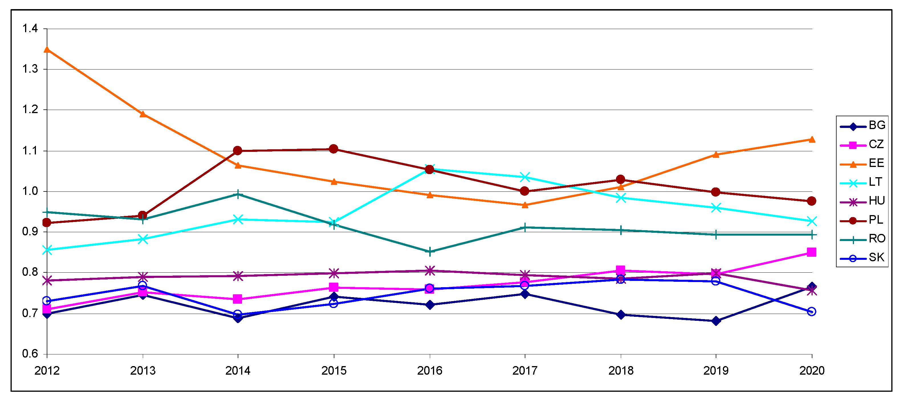
12	CompositeIndex	2020	0.7652	0.8500	1.1284	0.9279	0.7564	0.9748	0.8936	0.7037
		Aver	0.7150	0.7626	1.0861	0.9542	0.7933	1.0183	0.9189	0.7516
		Stdev	0.0269	0.0313	0.1272	0.0694	0.0081	0.0669	0.0411	0.0310
		Diff.	0.0502	0.0875	0.0423	−0.0263	−0.0369	−0.0435	−0.0253	−0.0480
		p_t	0.27	0.18	0.45	0.45	0.08	0.41	0.42	0.30

Aver. —average; Stdev—standard deviation; Diff.—the difference between 2020 and Aver (2012 ÷ 2019); p_t—probability from Student’s t-test that the difference was not significant.

presents the average values of the indicators for the year 2020, as well as the differences resulting from the evolution in each country. This analysis allows for the observation of the evolution of the countries at the level of the indicator used in the study.

In Table 7, the standard deviation was calculated to allow for estimation of the uniformity of the data set values. Thus, the standard deviations, based on the results obtained in most countries for most indicators, were small values between 0 and 0.01. These values allow us to say that the values of the data set are grouped around the mean value. Exceptions are recorded for the following indicators: ShResProd (HU (0.02)), RecyRatePk (PL(0.02)), RecyRateMn (PL and SK (0.03), BG (0.02), EE(0.02), LT(0.02) and RO(0.02)), CMatUseR (EE(0.04), CZ and PL each with 0.03)), ShTradeRwM (EE (0.03), RO (0.03) and PL (0.02)), ShPrivInvest (EE(0.07), RO(0.04), LT (0.03), HU and PL each with 0.02), ShGrAddVal (SK (0.02)), ShGasEmiss (EE (0.03) and LT (0.02)) and CompositeIndex (EE (0.13), LT and PL each with 0.07, RO (0.04), BG, CZ and SK each with 0.03). The values in the range 0.02–0.13, considered above as exceptions, allow us to say that they belong to those values of the data set that are further away from the average value.

From analysis of Table 7, the probability of observing such a difference (only positive or only negative, given by the t value = 1.96) between the true value and the average value in the sample is below the threshold to be considered significant. Thus, only in less than 12% of cases is the value of probability from Student’s t-test (p_t) for the RecyRatePk indicator higher than the one observed in RO in 2020. In less than 12% of cases, the value of probability from Student’s t-test (p_t) for the CMatUseR indicator is higher than that observed in BG in 2020. In less than 2% of cases, the value of probability from Student’s t-test (p_t) for CMatUseR is higher than that observed in SK in 2020, which cannot be attributed to chance (p_t < 5%). In less than 14% of cases, the probability value from Student’s t-test (p_t) for MatImportDep is lower than the one observed in EE in 2020. Among all countries, the value of the CompositeIndex for CZ in 2020 has the greatest distance from its average value corresponding to the previous period (2012–2019), with higher and lower values than could be recorded by chance in less than 18% of cases.

According to the results in Table 7, the ShMatFootp and ShResProd indicators show us that at the level of production and consumption of recycled materials, the values recorded in 2020 are stable in all the countries studied. Likewise, for the CMatUseR and ShTradeRwM indicators, the use of secondary materials to replace primary raw materials, in 2020 the recorded values show us continuity. According to the results recorded for the indicators mentioned above, we can say that hypothesis H1 is verified, and the process towards a circular economy is continuous in all countries.

To test hypothesis H2, we used indicators RecyRateEl, RecyRatePk and RecyRateMn, which, according to Table 7, show us that in 2020 each country continued the steps for waste management, these being selected by types of waste, and from comparison with the average of the past years the hypothesis is observed to be verified, the process being continuous.

Table 8. Analysis of the indicators’ variability according to direction.

Direction	Year/Country	BG	CZ	EE	LT	HU	PL	RO	SK
PC	2020	0.18	0.28	0.27	0.26	0.23	0.23	0.24	0.29
	Aver.	0.18	0.28	0.28	0.26	0.24	0.23	0.22	0.30
	Diff.	0.00	0.00	−0.01	0.00	−0.01	0.00	0.02	−0.01
WM	2020	0.38	0.42	0.37	0.41	0.34	0.38	0.25	0.45
	Aver.	0.40	0.42	0.37	0.42	0.37	0.35	0.30	0.37
	Diff.	−0.02	0.00	0.00	−0.01	−0.03	0.03	−0.05	0.08
SRM	2020	0.21	0.24	0.38	0.32	0.15	0.40	0.26	0.04
	Aver.	0.16	0.17	0.36	0.34	0.16	0.44	0.24	0.13
	Diff.	0.05	0.07	0.02	−0.02	−0.01	−0.04	0.02	−0.09
CI	2020	0.18	0.21	0.38	0.26	0.24	0.22	0.29	0.23
	Aver.	0.17	0.20	0.40	0.23	0.24	0.22	0.29	0.26
	Diff.	0.01	0.01	−0.02	0.03	0.00	0.00	0.00	−0.03
GSR	2020	0.20	0.30	0.27	0.32	0.22	0.25	0.13	0.30
	Aver.	0.19	0.31	0.32	0.30	0.22	0.22	0.12	0.30
	Diff.	0.01	−0.01	−0.05	0.02	0.00	0.03	0.01	0.00

PC—Production and Consumption; WM—Waste Management; SRM—Secondary Raw Materials; CI—Competitiveness and Innovation; GSR—Global Sustainability and Resilience; Aver. —average; Diff.—difference between 2020 and average.

shows the evolution of the countries by summing up the indicators presented in Table 7 according to the directions they belong to. This analysis is important because each country’s real progress towards a circular economy can be observed.

From the data presented in Table 8, the values in 2020 are equal to or above average for most countries, which illustrates positive evolution. For direction (1), the exceptions are EE, HU, and SK. For direction (2), the exceptions are RO, HU, BG, and LT. For direction (3), the exceptions are SK, PL, and LT. For direction (4), the exceptions are SK and EE. Lastly, for direction (5), the exceptions are EE and CZ. Consequently, when following the situation by country and comparing the year 2020 with the average of the eight previous studied years, one can notice that there is a decrease in the values recorded in the following countries for the given directions: BG (PC), CZ (GSR), EE (PC, CI, and GSR), LT (WM and SRM), HU (PC and WM), PL (SRM), RO (WM), and SK (SRM and CI).

The positive values recorded in direction (PM) “Production and Consumption” show the demand for and consumption of extractive materials, which in most countries was maintained or decreased. The exception is RO, where a slight increase was recorded.

In direction (WM) “Waste management”, the largest increase can be observed in 2020 compared to the average of the eight previous years. SK (0.08) is the country with the best recorded value, followed by PL (0.03). This increase exhibits a positive result because of these countries’ concern with collecting and recycling waste from electronic equipment, recycled plastic packaging and municipal waste. One can find a decrease in 2020 compared to the average in the following countries: RO (−0.05), HU (−0.03), BG (−0.02), and LT (−0.01).

In direction (SRM) “Secondary raw materials”, there is an increase in the following countries: CZ (0.07), BG (0.05), EE (0.02), and RO (0.02), which shows the share of recycled waste that is reintroduced into the economy through production in these countries. Negative results are found in SK (−0.09), PL (−0.04) and LT (−0.02).

In direction (CI) “Competitiveness and Innovation”, positive values are observed in countries such as LT (0.03), BG (0.01), and CZ (0.01), and negative results in SK (−0.03) and EE (−0.02). The positive results indicate gross investments in physical goods made by economic agents in the economy, and the increases in added value that are accelerators of development and economic growth.

In direction (GSR) “Global sustainability and Resilience”, the negative values recorded in the studied countries indicate efforts to reduce reliance on imports and reduce in greenhouse gas emissions from production activities. Thus, positive effects are observed: efforts of reduction compared to the average in countries such as EE (−0.05) and CZ (−0.01), but also efforts of maintenance in the other countries.

Table 9. The situations of the countries according to the achieved results.

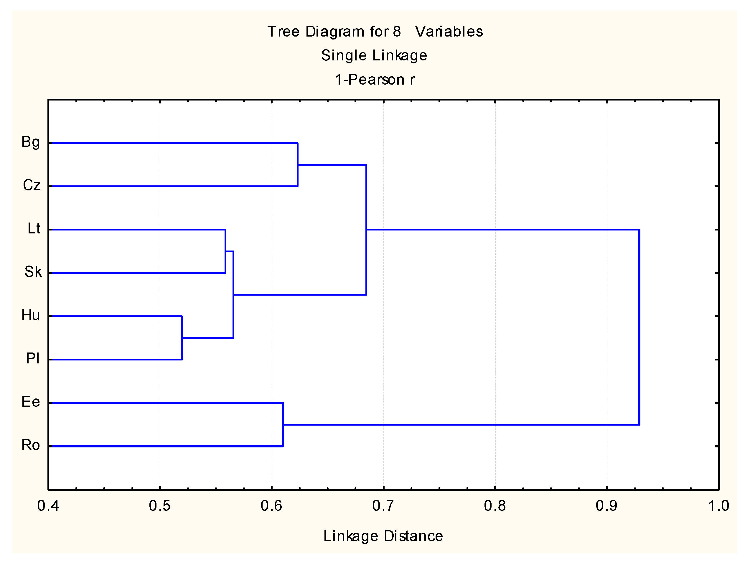
Country	PM	WM	SRM	CI	GSR	Composite Index	Level
BG	0.18	0.38	0.21	0.18	0.20	0.77	6
CZ	0.28	0.42	0.24	0.21	0.30	0.85	5
EE	0.27	0.37	0.38	0.38	0.27	1.13	1
LT	0.26	0.41	0.32	0.26	0.32	0.93	3
HU	0.23	0.34	0.15	0.24	0.22	0.76	7
PL	0.23	0.38	0.40	0.22	0.25	0.97	2
RO	0.24	0.25	0.26	0.28	0.13	0.89	4
SK	0.29	0.45	0.04	0.23	0.30	0.70	8

presents the information related to the year 2020 regarding the values recorded for the countries studied. This table shows the values obtained for each country, for each direction of study and for the total composite index.

From analysis of Table 9, after calculating the composite index, the best value obtained in 2020 is recorded for EE (1.13), followed by PL (0.97) and LT (0.93). Thus, these countries have made the most efforts to support the circular economy globally. The ranking of the countries is presented in the last column of Table 8.

At the level of the study directions, it can be observed that the best results are for (1) “Production and Consumption” in the countries SK, CZ, EE, for (2) “Waste management”—countries SK, CZ, LT, for (3) “Secondary raw materials”—PL and EE, for (4) “Competitiveness and Innovation” EE has the best result, and for (5) “Global sustainability and Resilience” RO has the best result.

After processing the data, the time series presented in Figure 1 resulted the following:

From analysis of the time series presented in Figure 1, EE was at a considerable distance from the other countries in 2012. In the following years, it was overtaken by PL (2014–2018) and LT (2016–2017), and in 2019 and 2020, EE regained the leading position.

In the years 2019–2020, PL was in 2nd place, followed by LT and RO. Countries such as CZ, HU, BG, and SK started from a similar approach in 2012, and in 2019 and 2020, only CZ and BG had an upward leap. In addition, from Figure 1 we can see that there are countries where the evolution is linear, but there are also countries where there were greater positive and negative oscillations over the years.

Afterwards, a cluster analysis was carried out, which is suitable to showcase the countries’ similarities and common skills because of the recorded evolution, namely regarding the approaches taken to transform each country’s economy into a circular economy (Figure 2).

In Figure 2, a plot was obtained using Pearson’s correlation coefficient, which shows the degree of linear association between two normally distributed variables under study, where the clusters and the values to which the clusters joined can be seen. Comparing the results obtained by measuring distance using the three measurement methods (Euclidean distance, 1-Pearson-r correlation coefficient and percentage of disagreement), similar results were obtained, confirming similarity or dissimilarity. As seen in Figure 2, the eight countries are grouped according to the values recorded into several clusters. For example, the smallest distance, and thus the greatest similarity, is between RO and EE, and compared to them, the greatest distance is between BG and CZ (over 0.9).

From Table 9, we see that analysis through the composite index allows us to classify the countries through their global result, and from Figure 2 we see the grouping of countries using the Pearson correlation, which shows us that hypothesis H3 is verified. This study groups countries according to the degree of similarity in their sustainable development, as countries with emerging market economies that are geographically located in a common area—Eastern Europe.

The study by Banjerdpaiboon et al. [58], involving the evaluation of six indicators of the circular economy (using multi-criteria decision-making tools), determines a classification by means of an efficiency score, which suggests that European countries are improving their overall performance in the CE, prioritizing improvement strategies that promote the recycling of biological waste and the rate of use of circular materials. Compared to the obtained super-efficiency score, which included RO, PL, LT in the efficient countries and HU, SK, EE, CZ and BG in the inefficient countries, our study indicated that the countries EE, PL, and LT were in the first places. These different results can be explained by the fact that the study mentioned above includes a smaller number of thematic study directions (3 instead of 5) and indicators (6 instead of 11); thus, the CE is approached from different perspectives.

The study by Lacko et al. [59] uses eight indicators (three for packaging recycling status, two for production and consumption of recycled materials, two related to the state of the national economy and one related to the state of organic agriculture) and uses models based on weakness results-oriented DEA CRS (CCR) and DEA VRS (BCC), including only the Visegrád Group countries. The study examines the differences between and successes of existing policies that have been implemented to improve CE status, and places the countries studied below the EU average, ranking them as follows: PL as closest to the EU average, followed by CZ, HU, and SK. Compared to our study, the study considers fewer countries (4 out of 8) with data from 2010–2017 compared to 2012–2020, and the indicators used to evaluate the circular economy are fewer (only 2 out of 11 are similar), the rest of the indicators being selected using other criteria specific to the study.

The study by Giannakitsidou et al. [60] measures environmental and CE performance in 26 EU countries by implementing data embedding analysis (through the DEA technique), using the three dimensions of the Social Progress Index as inputs and the recycling and/or cyclical use rate of materials as outputs. The study shows that the differences between Western and Eastern Europe have decreased, so among the Eastern European countries we have the following ranking: LT, PL, CZ, HU, BG, SK, EE, and RO. As in the studies mentioned above, the indicators used are different, especially in waste management, our study also having an approach with several indicators that define the circular economy.

Škrinjarić [61], in her study, uses a non-parametric approach (Grey Relational Analysis) and the results emphasize the link between CE and indicators such as GDP/capita, the corruption index and the government efficiency index, arguing that there is a link between these indicators at the level of the analyzed countries. Thus, she analyzes the period 2010–2016 and places the following countries first with positive results: LT, PL, EE, followed by HU, BG, SK, and RO. This study ranks the same countries in the top three places as in our study, even if the order is slightly different, the difference being caused by the types of indicators used in the study. Thus, although the study uses approximately the same thematic areas (4 out of 5), the indicators studied are fewer (6 out of 11), and for this reason the results may be different.

In our evaluation, the poor performances recorded by certain countries could be explained by the different choice of indicators and the extracted data (different periods) that might change the results of the analyses. Thus, we can say that the results are valid only for the given CE indicators specific to the given period.

4. Conclusions

Hypothesis (H1) “Is the production and consumption of recycled materials a continuous concern at the level of CE countries?” was verified by the results obtained for direction I “Production and Consumption” (in the indicators ShMatFootp and ShResProd) and direction III “Secondary Raw Materials” (in the indicators CmatUseR and ShTradeRwM). In direction I “Production and Consumption” it can be observed that, from comparison of the values from the year 2020 with the average of the years studied, in some countries the values are maintained (BG, CZ, LT and PL), in others they increase (RO), and a decrease of 0.01 is recorded in EE, HU and SK. For direction III “Secondary Raw Materials”, in some countries there is an increase: CZ, BG, EE and RO, and in others a decrease: SK, PL, LT and HU. From analysis of these two directions, we can conclude that the production and consumption of recycled materials is a continuing concern for the realization of CE.

Hypothesis (H2) “Does waste management allow for selection and direct contribution to CE?” was verified through direction II “Waste Management” (where the RecyRateEl, RecyRatePk and RecyRateMn indicators were identified). From analysis of the values from the year 2020 compared to the average of all years, it is found that the biggest increase is recorded in SK followed by PL, constant values in EE and CZ, and values lower than the average in RO, HU, BG, and LT. The three indicators within the “Waste Management” direction allow us to observe that there is a selection of waste according to type of waste, and in 2020 the highest values are found for municipal waste (BG, CZ, LT, PL and SK).

Hypothesis (H3) “Does the global result obtained by each country through the CE indicators allow for the classification and grouping of countries according to common characteristics?” was verified. The composite index allowed for the classification of countries, and cluster analysis allowed for the grouping of countries according to common characteristics. Thus, EE is the country that in the composite index significantly distances itself from the other countries in 2012 (1.35) and in 2020 (1.13); although the value decreased, it remained in first place. In RO, the value decreased from 2012 (0.95) to that recorded in 2020 (0.84) in the composite index, thus moving from second to fourth place. SK recorded a decrease in value from 2012 (0.73) to the value recorded in 2020 (0.70). HU in 2020 had the value of 0.76, compared to the value of 0.78 recorded in 2012. The cluster analysis reveals that the most similarities related to evolution are between EE and RO, BG and CZ, LT and SK, and HU and PL. Through the diagram using the Pearson correlation (Figure 2), it is possible to see the similarities that exist between countries due to the steps taken to facilitate the development of the policies necessary to achieve a circular economy.

The study carried out serves various decision-makers within each country who take steps towards sustainable development through circular economy. The benefits of a circular economy can be seen through the prism of sustainability of resources, extending the life of products, and informing users and customers on how to benefit as much as possible from products and production systems that use goods considered waste as resources.

There are several limitations to our work, some of which may be further investigated in the future. First, our model only investigates the CE situation, and the research can be extended to other situations. A possible extension would be to investigate how countries have progressed in each direction. Second, our paper analyzes data without being able to associate differences in values between countries with the socio-economic or political conditions that allowed these changes, this being impossible due to the existence of several variables.

References

- Gomonov, K.; Ratner, S.; Lazanyuk, I.; Revinova, S. Clustering of EU Countries by the Level of Circular Economy: An Object-Oriented Approach. Sustainability 2021, 13, 7158. [Google Scholar] [CrossRef]
- Dewulf, J.; Hellweg, S.; Pfister, S.; Leon, M.F.G.; Sonderegger, T.; de Matos, C.T.; Blengini, G.A.; Mathieux, F. Towards sustainable resource management: Identification and quantification of human actions that compromise the accessibility of metal resources. Resour. Conserv. Recycl. 2021, 167, 105403. [Google Scholar] [CrossRef]
- Razzaq, A.; Sharif, A.; Afshan, S.; Li, C.J. Do climate technologies and recycling asymmetrically mitigate consumption-based carbon emissions in the United States? New insights from Quantile ARDL. Technol. Forecast. Soc. Chang. 2023, 186, 122138. [Google Scholar] [CrossRef]
- Lenzen, M.; Geschke, A.; West, J.; Fry, J.; Malik, A.; Giljum, S.; Milà i Canals, L.; Piñero, P.; Lutter, S.; Wiedmann, T.; et al. Implementing the material footprint to measure progress towards Sustainable Development Goals 8 and 12. Nat. Sustain. 2022, 5, 157. [Google Scholar] [CrossRef]
- Shao, S.; Razzaq, A. Does composite fiscal decentralization reduce trade-adjusted resource consumption through institutional governance, human capital, and infrastructure development? Resour. Pol. 2022, 79, 103034. [Google Scholar] [CrossRef]
- Ke, J.; Jahanger, A.; Yang, B.; Usman, M.; Ren, F. Digitalization, financial development, trade, and carbon emissions; implication of pollution haven hypothesis during globalization mode. Front. Environ. Sci. 2022, 10, 211. [Google Scholar] [CrossRef]
- United Nations Development Programs. No More “Make, Take and Dispose”, USA. 2019. Available online: https://www.undp.org/blog/no-more-make-take-and-dispose (accessed on 8 August 2023).
- European Commission. A New Circular Economy Action Plan for a Cleaner and More Competitive Europe: COM/2020/98 Final; European Commission: Brussels, Belgium, 2020; Available online: https://environment.ec.europa.eu/strategy/circular-economy-action-plan_en (accessed on 5 November 2023).
- Golisano Institute for Sustainability. What Is Life Cycle Assessment (LCA)? RIT: Rochester, NY, USA, 2020; Available online: https://www.rit.edu/sustainabilityinstitute/blog/what-life-cycle-assessment-lca (accessed on 6 November 2023).
- Ghisellini, P.; Cialani, C.; Ulgiati, S. A Review on Circular Economy: The Expected Transition to a Balanced Interplay of Environmental and Economic Systems. J. Clean. Prod. 2016, 114, 11. [Google Scholar] [CrossRef]
- King, S.; Locock, K.E. A circular economy framework for plastics: A semi-systematic review. J. Clean. Prod. 2022, 364, 132503. [Google Scholar] [CrossRef]
- Geissdoerfer, M.; Savaget, P.; Bocken, N.M.P.; Hultink, E.J. The Circular Economy—A new sustainability paradigm? J. Clean. Prod. 2017, 143, 757. [Google Scholar] [CrossRef]
- Stahel, W. The circular economy. Nature 2016, 531, 435. [Google Scholar] [CrossRef]
- Chauhan, C.; Parida, V.; Dhir, A. Linking circular economy and digitalization technologies: A systematic literature review of past achievements and future promises. Technol. Forecast. Soc. Chang. 2022, 177, 121508. [Google Scholar] [CrossRef]
- Leal, J.M.; Pompidou, S.; Charbuillet, C.; Perry, N. Design for and from Recycling: A Circular Ecodesign Approach to Improve the Circular Economy. Sustainability 2020, 12, 9861. [Google Scholar] [CrossRef]
- Mazur-Wierzbicka, E. Towards Circular Economy—A Comparative Analysis of the Countries of the European Union. Resources 2021, 10, 49. [Google Scholar] [CrossRef]
- Ritzén, S.; Sandström, G.Ö. Barriers to the Circular Economy—Integration of Perspectives and Domains. Procedia CIRP 2017, 64, 7. [Google Scholar] [CrossRef]
- Bocken, N.M.P.; Olivetti, E.A.; Cullen, J.M.; Potting, J.; Lifset, R. Taking the circularity to the next level: A special issue on the circular economy. J. Ind. Ecol. 2017, 21, 476. [Google Scholar] [CrossRef]
- Kara, S.; Hauschild, M.; Sutherland, J.; McAloone, T. Closed-loop systems to circular economy: A pathway to environmental sustainability. CIRP Ann. 2022, 71, 505. [Google Scholar] [CrossRef]
- Su, B.; Heshmati, A.; Geng, Y.; Yu, X. A review of the circular economy in China: Moving from rhetoric to implementation. J. Clean. Prod. 2013, 42, 215. [Google Scholar] [CrossRef]
- Kirchherr, J.; Reike, D.; Hekkert, M. Conceptualizing the circular economy: An analysis of 114 definitions. Resour. Conserv. Recycl. 2017, 127, 221–232. [Google Scholar] [CrossRef]
- Szopik-Depczyńska, K.; Kędzierska-Szczepaniak, A.; Szczepaniak, K.; Cheba, K.; Gajda, W.; Ioppolo, G. Innovation in sustainable development: An investigation of the EU context using 2030 agenda indicators. Land Use Policy 2018, 79, 251. [Google Scholar] [CrossRef]
- Blum, N.U.; Haupt, M.; Bening, C.R. Why “circular” does not always mean “sustainable”. Resour. Conserv. Recycl. 2020, 162, 105042. [Google Scholar] [CrossRef]
- Moktadir, M.A.; Kumar, A.; Ali, S.M.; Paul, S.K.; Sultana, R.; Rezaei, J. Critical success factors for a circular economy: Implications for business strategy and the environment. Bus. Strategy Environ. 2020, 29, 3611. [Google Scholar] [CrossRef]
- Wang, H.; Masi, D.; Dhamotharan, L.; Day, S.; Kumar, A.; Li, T.; Singh, G. Unconventional path dependence: How adopting product take-back and recycling systems contributes to future eco-innovations. J. Bus. Res. 2022, 142, 707. [Google Scholar] [CrossRef]
- Fatimah, Y.A.; Govindan, K.; Murniningsih, R.; Setiawan, A. Industry 4.0 based sustainable circular economy approach for smart waste management system to achieve sustainable development goals: A case study of Indonesia. J. Clean. Prod. 2020, 269, 122263. [Google Scholar] [CrossRef]
- Chege, S.M.; Wang, D. The influence of technology innovation on SME performance through environmental sustainability practices in Kenya. Technol. Soc. 2020, 60, 101210. [Google Scholar] [CrossRef]
- Velenturf, P.M.; Purnell, P. Principles for a sustainable circular economy. Sustain. Prod. Consum. 2021, 27, 1437. [Google Scholar] [CrossRef]
- Martinho, V.J.P.D. Insights into circular economy indicators: Emphasizing dimensions of sustainability. Environ. Sustain. Indic. 2021, 10, 100119. [Google Scholar] [CrossRef]
- Zeng, H.; Chen, X.; Xiao, X.; Zhou, Z. Institutional pressures, sustainable supply chain management, and circular economy capability: Empirical evidence from Chinese eco-industrial park firms. J. Clean. Prod. 2017, 155, 54. [Google Scholar] [CrossRef]
- Malesios, C.; De, D.; Moursellas, A.; Dey, P.K.; Evangelinos, K. Sustainability performance analysis of small and medium sized enterprises: Criteria, methods, and framework. Socio-Econ. Plan. Sci. 2021, 75, 100993. [Google Scholar] [CrossRef]
- Amara, D.B.; Chen, H. Investigating the effect of multidimensional network capability and eco-innovation orientation for sustainable performance. Clean Technol. Environ. Policy 2020, 22, 1297. [Google Scholar] [CrossRef]
- Silvestre, B.S.; Tirca, D.M. Innovations for sustainable development: Moving toward a sustainable future. J. Clean. Prod. 2019, 208, 325. [Google Scholar] [CrossRef]
- Yuan, B.; Zhang, Y. Flexible environmental policy, technological innovation, and sustainable development of China’s industry: The moderating effect of environment regulatory enforcement. J. Clean. Prod. 2020, 243, 118543. [Google Scholar] [CrossRef]
- Govindan, K.; Shankar, K.M.; Kannan, D. Achieving sustainable development goals through identifying and analyzing barriers to industrial sharing economy: A framework development. Int. J. Prod. Econ. 2020, 227, 107575. [Google Scholar] [CrossRef]
- Borah, P.S.; Iqbal, S.; Akhtar, S. Linking social media usage and SME’s sustainable performance: The role of digital leadership and innovation capabilities. Technol. Soc. 2022, 68, 101900. [Google Scholar] [CrossRef]
- Smith, H.; Discetti, R.; Bellucci, M.; Acuti, D. SMEs engagement with the Sustainable Development Goals: A power perspective. J. Bus. Res. 2022, 149, 112. [Google Scholar] [CrossRef]
- Chari, M.D.; David, P. Sustaining superior performance in an emerging economy: An empirical test in the Indian context. Strateg. Manag. J. 2012, 33, 217. [Google Scholar] [CrossRef]
- Gu, W.; Zhao, X.; Yan, X.; Wang, C.; Li, Q. Energy technological progress, energy consumption, and CO2 emissions: Empirical evidence from China. J. Clean. Prod. 2019, 236, 117666. [Google Scholar] [CrossRef]
- Rosa, P.; Sassanelli, C.; Urbinati, A.; Chiaroni, D.; Terzi, S. Assessing relations between Circular Economy and Industry 4.0: A systematic literature review. Int. J. Prod. Res. 2019, 58, 1662–1687. [Google Scholar] [CrossRef]
- Schöggl, J.-P.; Rusch, M.; Stumpf, L.; Baumgartner, R.J. Implementation of digital technologies for a circular economy and sustainability management in the manufacturing sector. Sustain. Prod. Consum. 2023, 35, 401–420. [Google Scholar] [CrossRef]
- United Nations (UN). Transforming Our World: The 2030 Agenda for Sustainable Development; United Nations General Assembly: New York, NY, USA, 2015; Available online: https://sdgs.un.org/sites/default/files/publications/21252030%20Agenda%20for%20Sustainable%20Development%20web.pdf (accessed on 5 December 2023).
- European Commission (EC). Closing the Loop—An EU Action Plan for the Circular Economy; COM (2015) 614 Final, Brussels, 2.12.2015; European Commission: Brussels, Belgium, 2015; Available online: https://eur-lex.europa.eu/resource.html?uri=cellar:8a8ef5e8-99a0-11e5-b3b7-01aa75ed71a1.0012.02/DOC_1&format=PDF (accessed on 20 December 2023).
- Chertow, M.; Park, J. Scholarship and Practice in industrial symbiosis: 1989–2014. In Taking Stock of Industrial Ecology; Clift, R., Druckman, A., Eds.; Springer International: New York, NY, USA, 2016. [Google Scholar] [CrossRef]
- Gower, R.; Schroeder, P. Virtuous Circle: How the Circular Economy can Save Lives and Create Jobs in Low and Middle Income Countries; Tearfund and Institute of Development Studies: London, UK, 2016; Available online: https://www.researchgate.net/publication/306562812_Virtuous_Circle_how_the_circular_economy_can_create_jobs_and_save_lives_in_low_and_middle-income_countries#fullTextFileContent (accessed on 18 December 2023).
- Schroeder, P.; Anggraeni, K.; Weber, U. The Relevance of Circular Economy Practices to the Sustainable Development Goal. J. Ind. Ecol. 2018, 23, 77. [Google Scholar] [CrossRef]
- Schulte, A.; Kampmann, B.; Galafton, C. Measuring the Circularity and Impact Reduction Potential of Post-Industrial and Post-Consumer Recycled Plastics. Sustainability 2023, 15, 12242. [Google Scholar] [CrossRef]
- Pauliuk, S. Critical appraisal of the circular economy standard BS 8001:2017 and a dashboard of quantitative system indicators for its implementation in organizations. Resour. Conserv. Recycl. 2018, 129, 81–92. [Google Scholar] [CrossRef]
- Grdic, Z.S.; Nizic, M.K.; Rudan, E. Circular Economy Concept in the Context of Economic Development in EU Countries. Sustainability 2020, 12, 3060. [Google Scholar] [CrossRef]
- Busu, C.; Busu, M. Modeling the Circular Economy Processes at the EU Level Using an Evaluation Algorithm Based on Shannon Entropy. Processes 2018, 6, 225. [Google Scholar] [CrossRef]
- The World Business Council for Sustainable Development. Eco-Efficiency and Cleaner Production: Charting the Course to Sustainability. Available online: https://enb.iisd.org/consume/unep.html (accessed on 24 January 2024).
- Huppes, G.; Ishikawa, M.A. Framework for Quantified Eco-efficiency Analysis. J. Ind. Ecol. 2005, 9, 25–41. [Google Scholar] [CrossRef]
- Maxime, D.; Marcotte, M.; Arcand, Y. Development of eco-efficiency indicators for the Canadian food and beverage industry. J. Clean. Prod. 2006, 14, 636–648. [Google Scholar] [CrossRef]
- Eurostat Database. Available online: https://ec.europa.eu/eurostat/data/database (accessed on 2 August 2023).
- Bolboacă, S.D.; Jäntschi, L.; Sestras¸, A.F.; Sestras, R.E.; Pamfil, D.C. Pearson-Fisher Chi-Square Statistic Revisited. Information 2011, 2, 528. [Google Scholar] [CrossRef]
- Bálint, D.; Jäntschi, L. Missing Data Calculation Using the Antioxidant Activity in Selected Herbs. Symmetry 2019, 11, 779. [Google Scholar] [CrossRef]
- Jäntschi, L.; Gill, R. Chi Square Statistic. 2020. Available online: http://encyclopedia.pub/entry/81 (accessed on 15 August 2023).
- Banjerdpaiboon, A.; Limleamthong, P. Assessment of national circular economy performance using super-efficiency dual data envelopment analysis and Malmquist productivity index: Case study of 27 European countries. Heliyon 2023, 9, e16584. [Google Scholar] [CrossRef] [PubMed]
- Lacko, R.; Hajduová, Z.; Zawada, M. The Efficiency of Circular Economies: A Comparison of Visegrád Group Countries. Energies 2021, 14, 1680. [Google Scholar] [CrossRef]
- Giannakitsidou, O.; Giannikos, I.; Chondrou, A. Ranking European countries on the basis of their environmental and circular economy performance: A DEA application in MSW. Waste Manag. 2020, 109, 181–191. [Google Scholar] [CrossRef]
- Škrinjarić, T. Empirical assessment of the circular economy of selected European countries. J. Clean. Prod. 2020, 255, 120246. [Google Scholar] [CrossRef]