Coupling Relationship between Urbanization and Green Total Factor Productivity in the Context of Population Shrinkage: Evidence from the Rust Belt Region of China

Abstract

Northeast China, regarded as China’s Rust Belt, has been dealing with numerous issues related to societal transformation and ecological concerns. Data indicate that Northeast China has already become the most severely depopulated region. It is crucial for the region’s sustainable growth to figure out how to balance ecological and urban development in the face of population shrinkage. First, we measured the population shrinkage, urbanization, and green total factor productivity (GTFP) of each city. Second, we calculated the degree of coordination between urbanization and GTFP and spatially visualized it. Finally, we analyzed the influencing factors through further empirical evidence. The findings showed that Northeast China’s cities were generally becoming smaller in terms of population. Urbanization and GTFP both exhibited a climbing tendency, and overall coordination between the two grew gradually. The level of coordination declined as population shrinkage increased. Governmental, technological, and economic factors influenced the level of coordination. The role played by factors influencing coordinated development varied at different levels of shrinkage. The findings not only provide a new research perspective for understanding the coordinated development of socioeconomic and ecological environment in Northeast China, but also provide insights for further improving the relevant policies and promoting the sustainable development and transformation of the region.

1. Introduction

A vital stage of social progress is urbanization. Data from the WHO of the United Nations suggested that by 2050, urbanization would rise to 68% worldwide, with an urban population of 6.7 billion [1]. Such a large amount will inevitably cause shocks and disturbances to the resource and environmental carrying capacity. It has been documented that urbanization for economic growth in the past has put pressure on resources and ecology, including energy consumption [2,3], food and water scarcity [4,5], greenhouse gas production and climate systems [6,7], and changes in ecosystem functions [8,9]. Urbanization was physically rooted in resources and the environment, so cities inevitably underwent a transformation in the face of issues such as resource scarcity and ecological destruction. Facing the transition, the Rust Belt, a characteristic phenomenon of the world’s industrialization process, has been considered a typical region [10,11]. The term “rust belt” originates from the United States, which refers to an area characterized by deindustrialization, economic decline, population loss, and urban decay because of the shrinkage of industrial sectors, especially steelmaking, automobile manufacturing, and coal mining. In China, the Rust Belt mainly refers to the northeastern region [12]. As an old industrial base, the northeast assumed most of the industrial pressure in the early years of the founding of the country; however, overexploitation and irrational production methods have caused the northeast to face problems of environmental pollution, resource depletion, and industrial decline, which has led to increased ecological pressure, declining economic efficiency, and massive population loss. With the goal of achieving a social development that is sustainable and improves the well-being of people, it is crucial to balance the interaction between urbanization, resources, and natural environments in light of population shrinkage.

China’s sustained and rapid economic expansion depends on urbanization. China has experienced an enormous rise in urbanization since the reform and opening up. It has increased rapidly from 17.92% to 63.89% [13]; by 2050, the number is predicted to reach 76.0% [14]. However, behind the economic growth are problems such as resource consumption, environmental pollution, an increasing regional development gap, and imbalance in population distribution patterns. The entire driving force of regional socioeconomic and even naturally occurring ecological variables was responsible for population shrinkage, and it also had the opposite impact on the growth. The new urbanization driven by the increasing “shrinkage context” had a profound impact on urban socioeconomic development and interfered with urban green development and environmental health. This has given the subject of promoting urbanization and ecological environment coordination a new meaning. Investigating the realization of coordinated growth of urbanization and the environment has emerged as a hot topic of concern for society and academia, aiming at the major strategic needs of China’s modern urbanization and ecological civilization simultaneously.

The following aspects were the main emphases of the most recent research on the coordination between urbanization, resources, and environment. (1) A theoretical analysis and framework for the cooperation between urbanization and the environment’s ecological system. The relationship between cities and the environment had previously been researched in Western nations, mostly by the Environmental Kuznets Curve [15], the Circular Economy Theory [16], and the Decoupling Theory [17]. On this basis, China proposed the “Social-Economic-Natural” complex ecosystem theory [18], and further theoretical frameworks and technical routes were constructed to explain the coupling and role of the mechanisms of increasing urbanization along with ecological conditions [19,20], which provided a systematic research paradigm by analyzing from multiple perspectives. (2) The impact of urbanization on ecological environment and its analysis. Researchers used the ecological footprint, carbon emission, and eco-efficiency as eco-environmental representations to demonstrate the response and interrelationship between ecology and urbanization from a microscopic point of view. They selected the national, urban cluster, provincial, and municipal scales as study areas. The main arguments were as follows. First, urbanization improved resource utilization and restoration through technological innovation and economic investment, thus effectively improving ecological conditions [21,22]. Second, while urbanization promoted economic development, it caused waste of resources and environmental pollution, which damaged the ecological environment [23,24]. third, the relationship between urbanization and ecological environment is nonlinear due to the heterogeneity of the role of elements [25,26]. (3) The study of how urbanization and environmental issues interact ecologically. The interplay between human beings and the environment, which is complicated, nonlinear, and not certain, creates the social-ecological system [27]. They constructed a system of urbanization and ecological environment indicators, bringing the two under the same framework to explore the degree of their coordinated development. They also introduced an econometric model to analyze their spatial and temporal divergence and influence mechanisms [28,29,30,31]. Research focused on the dynamic evolution and feedback mechanisms of socioeconomic and ecological systems, leading to a comprehensive analysis of the elements of social and ecological systems [32,33]. Urbanization that respects ecological carrying capacity could prevent the ecological environment and cities from harming one another.

According to year-by-year population data comparisons, Northeastern China continues to suffer from population loss, and most of the outflow is from the young and middle-aged labor force, leading to changes in the local demographic structure and making the problem of population shrinkage even more significant [34,35]. In light of this, this article used samples from cities in Northeast China, focusing on the two themes of urbanization as well as resources and the environment, and empirically studied the spatial and temporal evolution patterns of urbanization and GTFP coordination levels in 34 cities in Northeast China under the context of population shrinkage and quantified the key influencing factors. The innovations of the paper are the following. (1) In the background of the study, population shrinkage is innovatively taken as the premise of the study, and different degrees of shrinkage are classified to measure regional heterogeneity. (2) The object of the study is to select a typical rust belt region in China, the three northeastern provinces, and to refine the perspective to the prefecture-level city level. (3) In terms of research content, we include GTFP in the research framework as a system that refines the input and output of resources and the environment in the coupled system of urbanization and ecological environment. This study provides important practical implications for the implementation of urban green, low-carbon, and ecological development strategies.

2. Materials and Methods

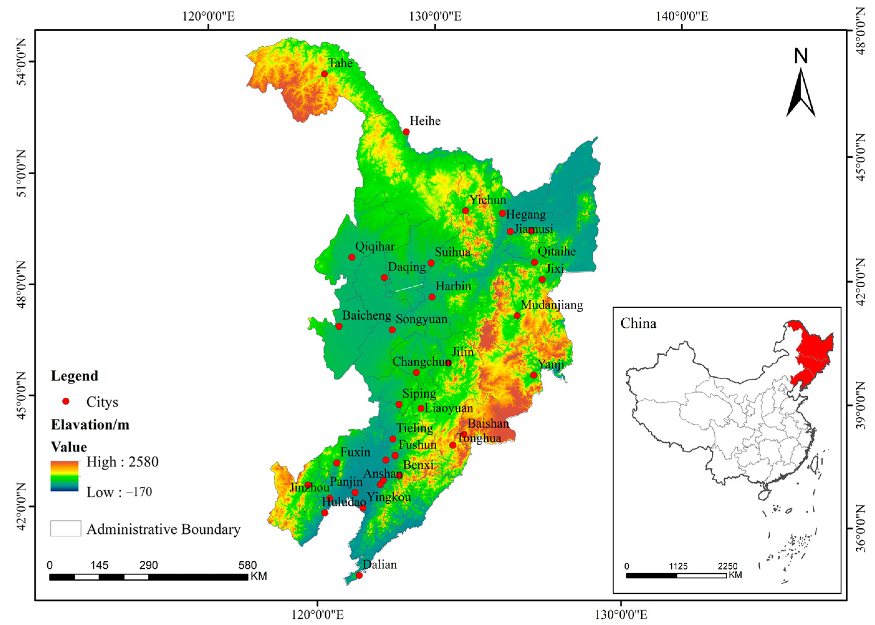
2.1. Study Area and Data Source

This study took Northeast China (Figure 1), the rust belt of China [36], as the research object. Russia borders the northeast region to the north and the Korean Peninsula to the east, and it neighbors the Beijing-Tianjin-Hebei city cluster and the Bohai Rim metropolitan area, which is the gateway of China to the outside world. Northeast China mainly includes Heilongjiang, Jilin, and Liaoning provinces. It spans 118–135° E longitude and 48–55° N latitude and includes two national city clusters, Harbin-Changchun urban agglomeration and Central and Southern Liaoning area. Northeast China boasts abundant permafrost, wetlands, forests, minerals, and agricultural products, and it is renowned for its well-developed heavy industries. The northeast region’s development, however, has stalled due to the depletion of resources such as minerals and forests and the rigidity of the industrial structure. According to statistics, the GDP of Northeast China is 5.6 trillion yuan in 2021, accounting for only 4.9% of China’s GDP. The profound changes in economic and social structure have led to a massive exodus of population from the northeast region, with approximately 11.11 million people leaving Northeast China in the 2010s, according to the sixth and seventh censuses of China [30,35,37]. Therefore, in order to revitalize the development of the old industrial bases in Northeast China and provide some theoretical value for achieving sustainable regional development, it is crucial to explore the coordinated interaction among urbanization along with resources and the environment in this region.

In this paper, 34 prefecture-level cities in Northeast China were used as the basic study area (among which Da Hinggan Ling Prefecture and Yanbian Korean Autonomous Prefecture were excluded from this paper due to missing data). The sixth and seventh National Censuses were used as the nodes, and the time period of the full 10-year span was selected. Population data were obtained from the sixth and seventh National Census data, and all other data used were directly or indirectly obtained from the 2011–2021 China Cities Statistical Yearbook. Data on population urbanization dimension were missing for individual years and were supplemented using interpolation. To counteract the impact of inflation, the pricing statistics were deflated.

2.2. Construction of Index System

2.2.1. Index System of Population Shrinkage

Population shrinkage is the result of many factors such as declining industrial structure, weakened regional competitive advantages, and depleted resources [38]. In this paper, four indicators were selected to comprehensively measure the degree of population shrinkage, including total population change, change in the proportion of population aged 0–14 years, change in the aging rate, and change in the natural growth rate, to build an index system for evaluating the degree of population shrinkage (

Table 1. Index system of the population shrinkage.

System	Subsystem	Indicators	Attribute
Shrinkage degree of Northeast China	Degree of demographic change	Total population change	+
	Tendency of demographic change	Change in the proportion of population aged 0–14	+
		Ageing rate change	−
		Change in natural growth rate	+

). Among them, the change of total population directly reflected the population loss in the three northeastern provinces, while the change in population aged 0–14, aging rate, and natural growth rate indicated the population development potential and laterally reflected the population development trend.

2.2.2. Index System of Urbanization

Urbanization is a process of economic and social development in which the rural population migrates to cities and towns, nonagricultural industries and production and lifestyles gather in cities and towns, infrastructure and social security spread to cover rural areas, and the scale of cities and towns gradually expands. In this study, the researchers used 20 variables across five perspectives (population, economy, society, space, and ecology) to construct the urbanization evaluation index system (

Table 2. Index system of urbanization.

System	Subsystem	Indicators, Unit	Attribute
Population urbanization	Population agglomeration	Proportion of urban population to total population, %	+
	Employment structure	Proportion of tertiary industry workers, %	+
		Urban registered unemployment rate, %	−
	Educational level	Share of students in higher education, %	+
Economic urbanization	Economic scale	GDP per capita, yuan	+
		Per capita disposable income of urban residents, yuan	+
	Industry structure	The proportion of tertiary industry in GDP, %	+
Socialurbanization	Medical and cultural level	Number of beds in medical and health institutions, 10,000 people	+
		Number of health technicians, 10,000 people	+
		Public library collections, 10,000 people	+
	Basic guarantee	Medical insurance coverage, %	+
		Share of education spending, %	+
		Internet penetration rate, %	+
Spatialurbanization	Land use	Proportion of construction land, %	+
	Infrastructure	Urban road area per capita, m2	+
		Number of public transport vehicles, 10,000 people	+
Ecological urbanization	Ecological restoration	Greening coverage rate of built-up area, %	+
		Parkland per capita, m2	+
	Pollution control	Sewage treatment rate, %	+
		Harmless disposal rate of domestic waste, %	+

). Population urbanization was the process of improving the size as well as the quality of the urban population; economic urbanization was the process of economic factors gathering in the tertiary industry and the development of urban economic level; social urbanization referred to the improvement of life quality and public services; spatial urbanization was the increase in the size of cities and the development of better infrastructure; ecological urbanization referred to the process of green urban development and improvement of the human living environment.

2.2.3. Index System of GTFP

In contrast to conventional total factor productivity, GTFP places equal emphasis on economic growth, energy saving, reduction of emissions, and sustainable environmental protection. This paper selected seven indicators in three criterion levels of input, desired output, and non-desired output to build a GTFP index system (

Table 3. Index system of green total factor productivity (GTFP).

System	Subsystem	Indicators, Unit	Attribute
Inputs	Capital investment	Capital stock of fixed assets, billion yuan	+
	Labor input	Number of employees, millions	+
	Energy input	Energy consumption, kW·h	+
Outputs	Expected output	Regional GDP, billion yuan	+
	Non-desired outputs	Industrial wastewater discharge, tons	−
		Industrial sulfur dioxide emissions, tons	−
		Industrial dust emissions, tons	−

). The inputs were divided into capital, labor, and energy, which referred to the basic condition of environmental protection; the desired output was the real gross product, which indicated the ideal result of green development in each city. The non-desired outputs were industrial wastewater, industrial sulfur dioxide, and industrial soot emissions, which were aspects that still needed improvement in the green development process.

2.3. Research Methods

2.3.1. Entropy-Weighting Method

The entropy weight method originated from the definition of physics. According to the interpretation of the basic principles of information theory, information is used to measure the degree of order in a system, and entropy is used to measure the degree of disorder in a system. Accordingly, the entropy value can be used to determine the degree of dispersion of an indicator. Specifically, the smaller the value of information entropy, the greater the degree of dispersion of the indicator. The article adopts the entropy weight method to measure the urbanization index, and the equations are as follows:

$$p_{ij}=\frac{x_{ij}}{{\sum }_{i=1}^m{x}_{ij}}$$

(1)

$$e_j=\left(-\frac{1}{lnm}\right)\sum _{i=1}^m{p}_{ij}\times {lnp}_{ij}$$

(2)

$$w_j=\frac{\left(1-e_j\right)}{{\sum }_{j=1}^n\left(1-e_j\right)}$$

(3)

First, calculate the proportion (p_ij) of the j-indicator for city i. Second, calculate the entropy (e_j) of the j-indicator. Third, calculate the entropy weight of j-indicator (w_j), where x_ij is the original j-indicator value of city i; m is the number of cities; n is the number of indicators.

2.3.2. SBM-ML Index

The SBM-ML index incorporates inputs, desired outputs, and non-desired outputs into the theoretical framework of the directed distance function. First, it estimates the effective production frontier of an economy by using the data envelopment method. Second, it measures the distance by the DDF between each economic production decision-making unit and the effective production frontier, and, finally, the ML productivity index for the period based on the DDF of the two periods.

First, we defined a model of environmental technology that took resource constraints into account. The range of manufacturing options that provided the foundation for measuring GTFP was offered by environmentally friendly technology. It might be implied in the form of an output set as in Equation (4), assuming that the desired output vector was y, the undesired output vector was b, and the input vector was χ.

$$P\left(\chi \right)=\left\{\left(y,b\right),\chi ϵR_{+}^{*}\right\}$$

(4)

Assuming that at some point t, the observations of inputs and outputs for the K decision units were $({\chi }_k^t,y_k^t,b_k^t)$, k = 1, 2, …, K; t = 1, 2, …, T, and the set of outputs determined from these observations that satisfy the assumptions were:

$$P\left({\chi }^t\right)=\left\{\begin{array}{c}\begin{array}{c}\left(y^t,b^t\right):{\displaystyle \sum _{k=1}^K}{\lambda }_k^t{y}_{km}^t\ge y_{mt},m=\mathrm{1,2},\cdots ,M;\\ {\displaystyle \sum _{k=1}^K}{\lambda }_k^t{b}_{ki}^t\ge b_i^t,i=\mathrm{1,2},\cdots ,I;\\ {\displaystyle \sum _{k=1}^K}{\lambda }_k^t{\chi }_{kn}^t\ge {\chi }_n^t,n=\mathrm{1,2},\cdots ,N;\\ {\lambda }_k^t\ge 0,k=\mathrm{1,2},\cdots ,K\end{array} \end{array}\right.$$

(5)

The distance function can be viewed in economics as the proportion of a given production decision unit that approaches the optimal production point in an ideal state. The directional distance function promotes paralleled expansion of the desired output and the undesirable output in the direction of the efficient production frontier in order to reduce frontier shrinkage, which can be achieved by increasing output and decreasing inputs on the trajectory specified by the chosen directional vector. The directional distance function was defined as:

$$\begin{array}{c}\overrightarrow{D_0}\left(\chi ,y,b;g_y,{-g}_b\right)=\mathit{sup}\left\{\beta :\left(y+\beta g_y,b-\beta g_b\right)ϵP\left(\chi \right)\right\}\end{array}$$

(6)

In Equation (6), g was the direction vector, and $\mathrm{g}=(g_y,-g_b)$ was the distance function value. β represented the maximum multiple of the expansion of the output vector (y,−b) that can be achieved without adding other inputs, i.e., under the original input vector χ, along the direction vector g. β represented the separation of the production decision-making unit (DMU) from the frontier of efficient production; the smaller β was, the closer the DMU was to the efficient production frontier, and the more efficient that DMU was; when β = 0, it meant that the DMU was on the efficient production frontier, indicating that its production was technologically efficient.

$$\begin{gathered} \left\{\begin{array}{c}\overrightarrow{D_0^t}\left({\chi }_0^t,y_0^t,b_0^t;y_k^t,{-b}_k^t\right)=\mathit{max}\beta ;\\ {\displaystyle \sum _{k=1}^k}{\lambda }_k^t{y}_{km}^t\ge \left(1+\beta \right)y_{km}^t;\\ {\displaystyle \sum _{k=1}^k}{\lambda }_k^t{b}_{ki}^t=\left(1-\beta \right)b_{ki}^t;\\ {\displaystyle \sum _{k=1}^k}{\lambda }_k^t{\chi }_{kn}^t\le {\chi }_{kn}^t;{\lambda }_k^t\ge 0\end{array}\right. \\ S=\mathrm{1,2},\cdots ,S;m=\mathrm{1,2},\cdots ,M;n=\mathrm{1,2},\cdots ,N;k=\mathrm{1,2},\cdots ,K \end{gathered}$$

(7)

In Equation (7), using N factor inputs: $\mathsf{\chi }=\left({\mathsf{\chi }}_1,\dots ,{\mathsf{\chi }}_N\right)\in R_N^{+}$; producing M desired outputs: $\mathrm{y}=\left({\mathrm{y}}_1,\dots ,{\mathrm{y}}_M\right)\in R_M^{+}$; producing I non-desired outputs: $\mathrm{b}=\left({\mathrm{b}}_1,\dots ,{\mathrm{b}}_I\right)\in R_I^{+}$; ${\mathsf{\lambda }}_k^t$ denoted the weight of each cross-section observation. K = 1, 2, …, K represented the decision unit. t = 1, 2, …, T represents the period.

The GTFP could be built using the directional distance function, and the output-based ML productivity index was based on definition of productivity change between periods t and (t + 1):

$${ML}_t^{t+1}=\{\frac{\left[1+\overrightarrow{D_0^t}\left({\chi }^t,y^t,b^t;y^t,{-b}^t\right)\right]}{\left[1+\overrightarrow{D_0^t}\left({\chi }^{t+1},y^{t+1},b^{t+1};y^{t+1},{-b}^{t+1}\right)\right]}\times \frac{\left[1+\overrightarrow{D_0^{t+1}}\left({\chi }^t,y^t,b^t;y^t,{-b}^t\right)\right]}{\left[1+\overrightarrow{D_0^{t+1}}\left({\chi }^{t+1},y^{t+1},b^{t+1};y^{t+1},{-b}^{t+1}\right)\right]}{\}}^{\frac{1}{2}}$$

(8)

Finally, the ML index was multiplied cumulatively to obtain the final GTFP [39].

2.3.3. CCD Model

The coupling coordination degree (CCD) model could not only measure the degree of interaction between urbanization and GTFP but also analyze the coordinated development trend between the two. In this paper, on the basis of measuring the coupling degree of the two systems, the CCD model was introduced, and the calculation steps were as follows:

$$\begin{gathered} \begin{array}{c}\begin{array}{c}C=\sqrt{U_1{U}_2/{\left[0.5\left(U_1+U_2\right)\right]}^2}\end{array}\end{array} \\ \begin{array}{c}\begin{array}{c}T=a{U}_1+b{U}_2, a+b=1\end{array} \end{array} \\ \begin{array}{c} D=\sqrt{C\times T}\end{array} \end{gathered}$$

(9)

where C indicated the coupling degree of urbanization and GTFP; U₁ and U₂ indicated urbanization and GTFP; And D indicated the CCD of urbanization and GTFP. T was the comprehensive coordination index, while a and b indicated the weights of urbanization and GTFP. a = b = 0.5 as the two systems were usually considered equally important. In addition, referring to the existing research [40], the CCD was split into 10 levels (

Table 4. Coordinated development stage classification of urbanization and GTFP.

	D Range	Coordination Level		D Range	Coordination Level
1	0 ≤ D ≤ 0.1	Extreme disorder	6	0.5 < D ≤ 0.6	Barely coordinated
2	0.1 < D ≤ 0.2	Severe disorder	7	0.6 < D ≤ 0.7	Primary coordination
3	0.2 < D ≤ 0.3	Moderate disorder	8	0.7 < D ≤ 0.8	Intermediate coordination
4	0.3 < D ≤ 0.4	Mild disorder	9	0.8 < D ≤ 0.9	Good coordination
5	0.4 < D ≤ 0.5	On the verge of disorder	10	0.9 < D ≤ 1.0	Quality coordination

).

2.3.4. Spatial Autocorrelation Analysis

The spatial distribution of the coupled and coordinated level of urbanization and GTFP in the Northeast China was analyzed for nonrandom agglomeration by means of Global Moran’s I, which measures global spatial autocorrelation. The calculation equation was as follows:

$$\begin{array}{c}I=\frac{{\sum }_{i=1}^n{\sum }_{j=1}^n{w}_{ij}\left(x_i-\overline{x}\right)\left(x_j-\overline{x}\right)}{S^2{\sum }_{i=1}^n{\sum }_{j=1}^n{w}_{ij}}, S^2=\frac{{\sum }_{i=1}^n{\left(x_i-\overline{x}\right)}^2}{n}\end{array}$$

(10)

where x_i and x were the CCD of urbanization and GTFP of cities i and j, respectively; $\overline{\mathrm{x}}$ was the average value of the CCD; n was the total number of spatial elements, i.e., the number of city samples; S² was the spatial element variance; and w_ij was the (i,j) element of the spatial weighting matrix, which was used to measure the distance between city i and city j. Moran’s I take values between [−1, 1], greater than 0 indicates positive spatial autocorrelation, less than 0 indicates negative spatial autocorrelation, and equal to 0 indicates no spatial autocorrelation.

2.3.5. Spatial Econometric Model

SDM is a model in spatial econometrics that is used to analyze the geospatial dependence of data. The model is able to deal with the interactions and effects of individuals or regions in the spatial dimension. As the article needed to solve the complex spatial autocorrelation problem in the regression model, the SDM model assumed that the value of the dependent variable would be influenced by the independent variables of neighboring regions besides the local independent variables. After comprehensive analysis, the SDM model was adopted in this study to measure the influencing factors and the spillover effect of the coordinated level of urbanization and GTFP. Finally, the analysis of heterogeneity was carried out, and a replacement spatial matrix was adopted for the robustness test to prove the reliability of the conclusions.

3. Results

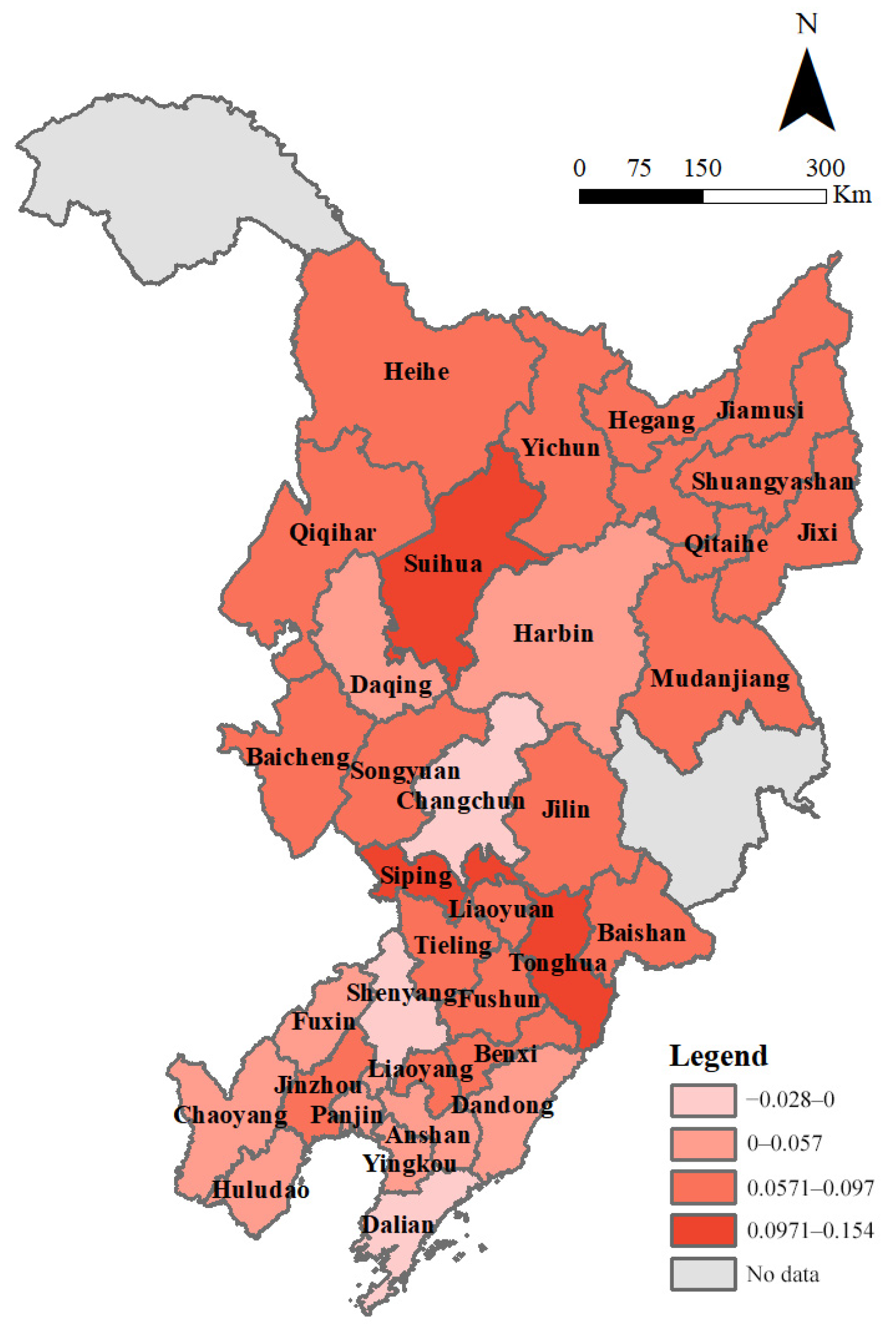
3.1. Measurement of Urban Population Shrinkage

Each prefecture-level city’s shrinking population index was determined using the weighted synthesis method, which was combined with the natural discontinuity grading method [41] in the ArcGIS 10.7 spatial analysis software to classify the city into four grades according to the degree of population shrinkage and visualized and expressed (Figure 2 and

Table 5. Classification of cities by degree of shrinkage.

Type	Cities	Corresponding Total Population Change Rate Range
Non-shrinking cities (−0.028–0)	Changchun, Shenyang, Dalian	>0
Mildly shrinking cities (0–0.057)	Panjin, Yingkou, Daqing, Chaoyang, HarbinHuludao, Anshan, Fuxin, Dandong	−10%~0
Moderately shrinking cities(0.0571–0.097)	Hegang, Tieling, Jinzhou, Liaoyang, Jiamusi, Liaoyuan, Shuangyashan, Mudanjiang, Jixi, Jilin, Fushun, Yichun, Songyuan, Benxi, Heihe, Baicheng, Qiqihar, Baishan, Qitaihe	−30%~−10%
Severely shrinking cities(0.0971–0.154)	Suihua, Tonghua, Siping	<−30%

).

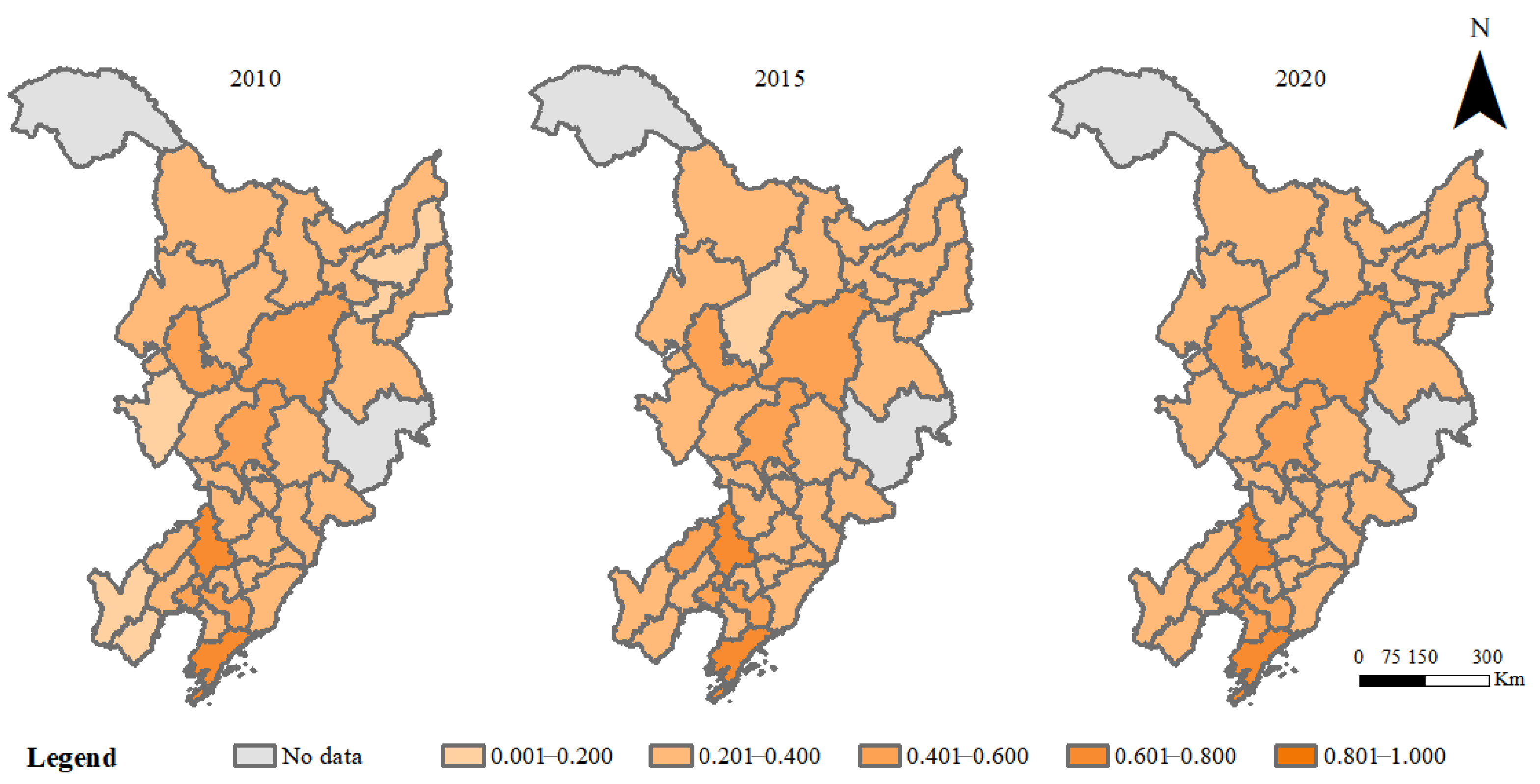
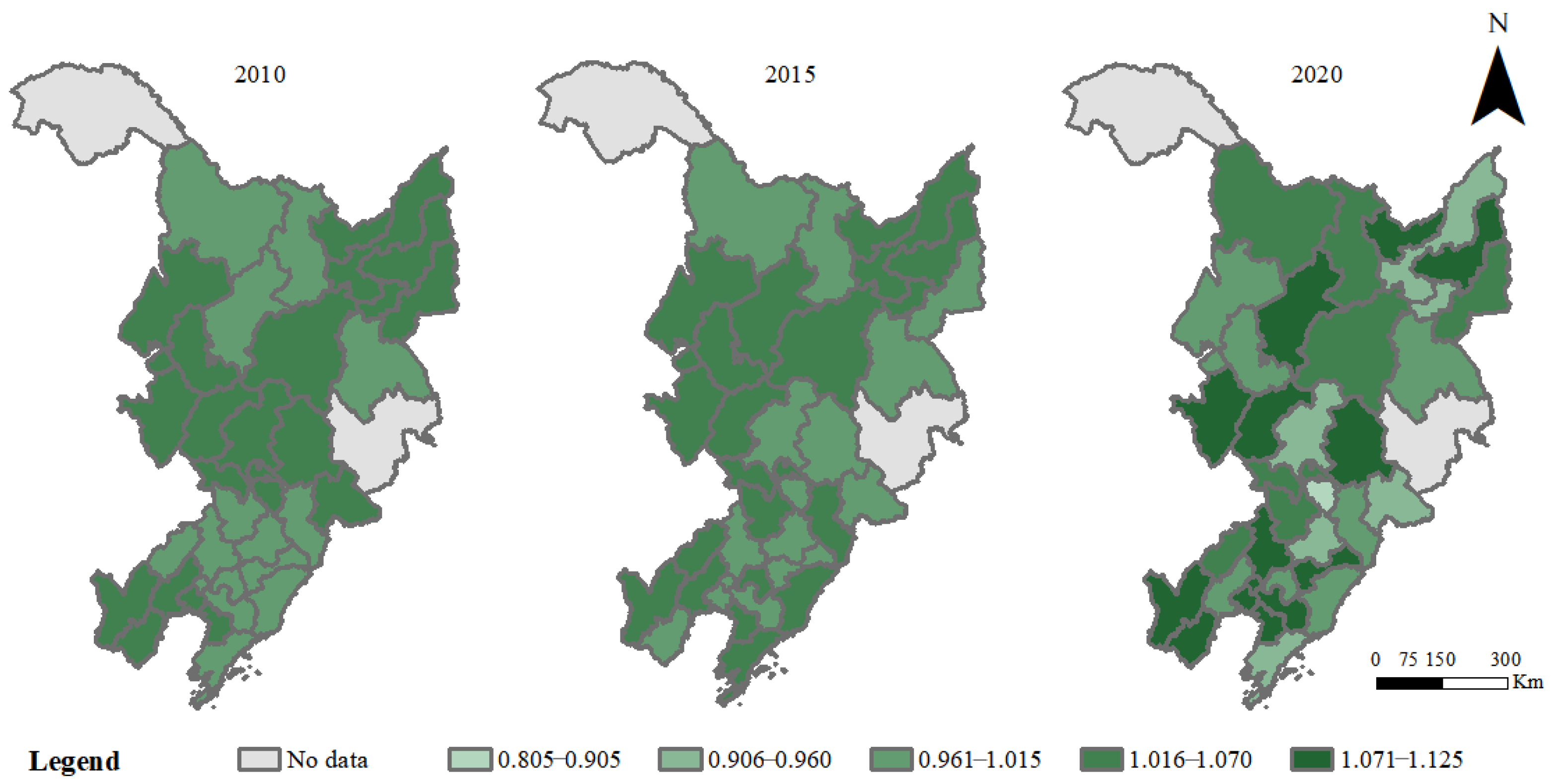
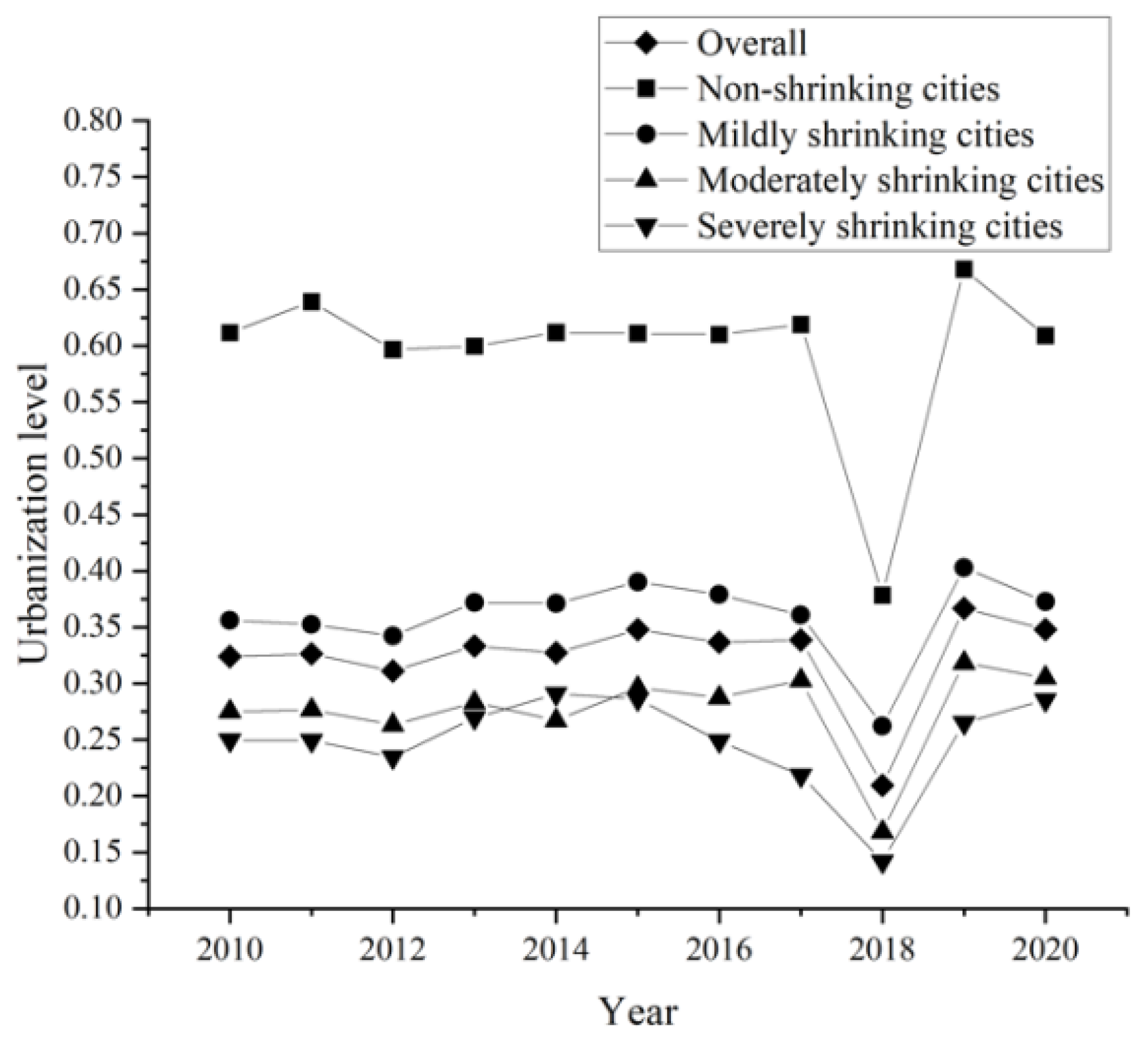
3.2. Measurement of Urbanization and GTFP

The urbanization index of each city was measured using the entropy-weighting method by adopting comprehensive indicators. The GTFP was measured using Equation (8), and the changes in the spatial pattern of urbanization and GTFP in each city were visualized using ArcGIS (Figure 3 and Figure 4); in order to increase the comparability of the data, the three selected time nodes were classified using uniform classification standards (the same below).

Urbanization: As can be seen from Figure 3, the urbanization level of the three northeastern provinces has increased from 0.3239 to 0.3481 during the study period, showing an overall upward trend, mainly in the transition from a low level to a medium-to-high level, which resulted from the increase in local financial income and the improvement of public facilities. Spatially, it was characterized by the “core-edge” pattern with Harbin-Changchun and Shenyang-Dalian as the center and spreading around. Among them, Shenyang and Dalian have maintained a high value above 0.6, and a low value below 0.2 has been found in the western part of Liaoning, in areas within the “siphon” range of the central city, and in the northeastern part of Heilongjiang, which lies on the border, with disparities in the level of development still existing between the regions.

GTFP: Figure 4 illustrates that the region’s general foundation was stable, mostly in the middle to high value range of 0.961 to 1.125. However, it was worth noting that the GTFP of individual cities fluctuated in 2020, such as Changchun, which has dropped from the 0.961 to 1.015 range to the 0.096 to 0.960 range, with a slight downward trend, which was related to the increase in pollution emissions. The level of GTFP in resource-based cities has increased significantly, such as Hegang, Shuangyashan, and other areas, jumping to the forefront, indicating that the transformation has had preliminary results.

Classified by different degrees of shrinkage, it can be seen from Figure 5 that, except for 2018 when the index fell off a cliff due to a change in the statistical caliber, the urbanization level of the three northeastern provinces from 2010 to 2020, although slightly fluctuating, showed an overall upward trend. Among them, as shown in

Table 6. Results of urbanization level and GTFP measurement in cities with different degrees of shrinkage.

Cities	2010		2020		Average
	Urbanization	GTFP	Urbanization	GTFP	Urbanization	GTFP
Overall	0.3239	1.0159	0.3481	1.0290	0.3245	1.0110
Non-shrinking cities	0.6116	1.0014	0.6090	1.0051	0.5959	1.0047
Mildly shrinking cities	0.3561	1.0235	0.3728	1.0616	0.3602	1.0148
Moderately shrinking cities	0.2749	1.0159	0.3051	1.0167	0.2766	1.0111
Severely shrinking cities	0.2498	1.0075	0.2852	1.0329	0.2491	1.0048

, non-shrinking cities were much higher than shrinking cities, and urbanization levels decreased with increasing shrinkage. As can be seen from Figure 6, the overall difference in GTFP was not large, with mildly shrinking cities and moderately shrinking cities experiencing relatively smooth changes during the period of examination, and non-shrinking cities and severely shrinking cities experiencing larger changes. Among them, cities with mild shrinkage had higher levels of GTFP, and most of these cities were located in the periphery of the core cities, upgrading their industries through the scale effect, absorbing resources and technologies, and practicing green production and development. In terms of development trends, there was an overall upward trend, but there was a tendency for non-shrinking cities to decrease, and among the shrinking cities, there was a clear upward trend in the mildly shrinking and severely shrinking cities, which was related to the implementation of their transformation policies.

3.3. Analysis of the CCD of Urbanization and GTFP under Different Population Shrinkage Contexts

The CCD of urbanization and GTFP was measured for each city using Equation (9), and, on this basis, the cities were divided according to different levels of shrinkage (

Table 7. Type of coordination between urbanization and GTFP.

Cities	2010		2020
	D	Coordination Level	D	Coordination Level
Overall	0.7469	Intermediate coordination	0.7669	Intermediate coordination
Non-shrinking cities	0.8829	Good coordination	0.8827	Good coordination
Mildly shrinking cities	0.7665	Intermediate coordination	0.7888	Intermediate coordination
Moderately shrinking cities	0.7224	Intermediate coordination	0.7434	Intermediate coordination
Severely shrinking cities	0.7071	Intermediate coordination	0.7345	Intermediate coordination

).

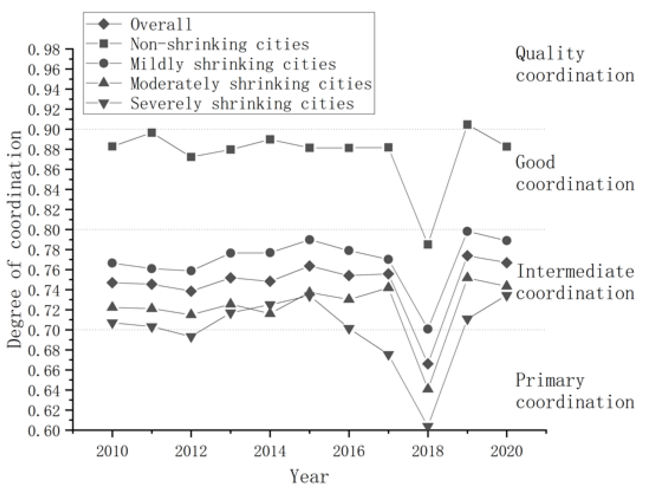
3.3.1. Temporal Characterization Analysis

Overall, the CCD between urbanization and GTFP in the northeast region from 2010 to 2020 concentrated in the medium degree of coordination (0.7469–0.7669). Each city maintained or advanced by one step throughout this time, demonstrating a gradual transition from “primary” to “intermediate.” The average coordination level of the 34 cities had increased from 0.7469 to 0.7669 (Table 7). In 2010, the CCD of each city ranged from 0.6287 to 0.9105, which was in the range of primary coordination to high-quality coordination, with the lowest value appearing in Chaoyang (0.6287) and the highest appearing in Dalian (0.9105). The coordination level of cities in 2020 ranged from 0.6823 to 0.9157, with the minimum occurring in Songyuan (0.6823) and the maximum in Shenyang (0.9157). The coordination level of 10 cities slightly decreased during the study period, with Liaoyuan having the largest decrease of 9.13%; the coordination level of 24 cities increased, with Shuangyashan having the largest increase of 16.45%. From the point of view of different degrees of shrinkage, the overall coordination level showed fluctuating and rising changes except in 2018 (Figure 7). Cities that were not shrinking or were just slightly shrinking had coordination levels that were higher than a median, ranging from 0.8827 to 0.8829, which was significantly higher than that of cities with shrinking population. In shrinking cities, the coordination level continued to decline as the degree of shrinkage increased.

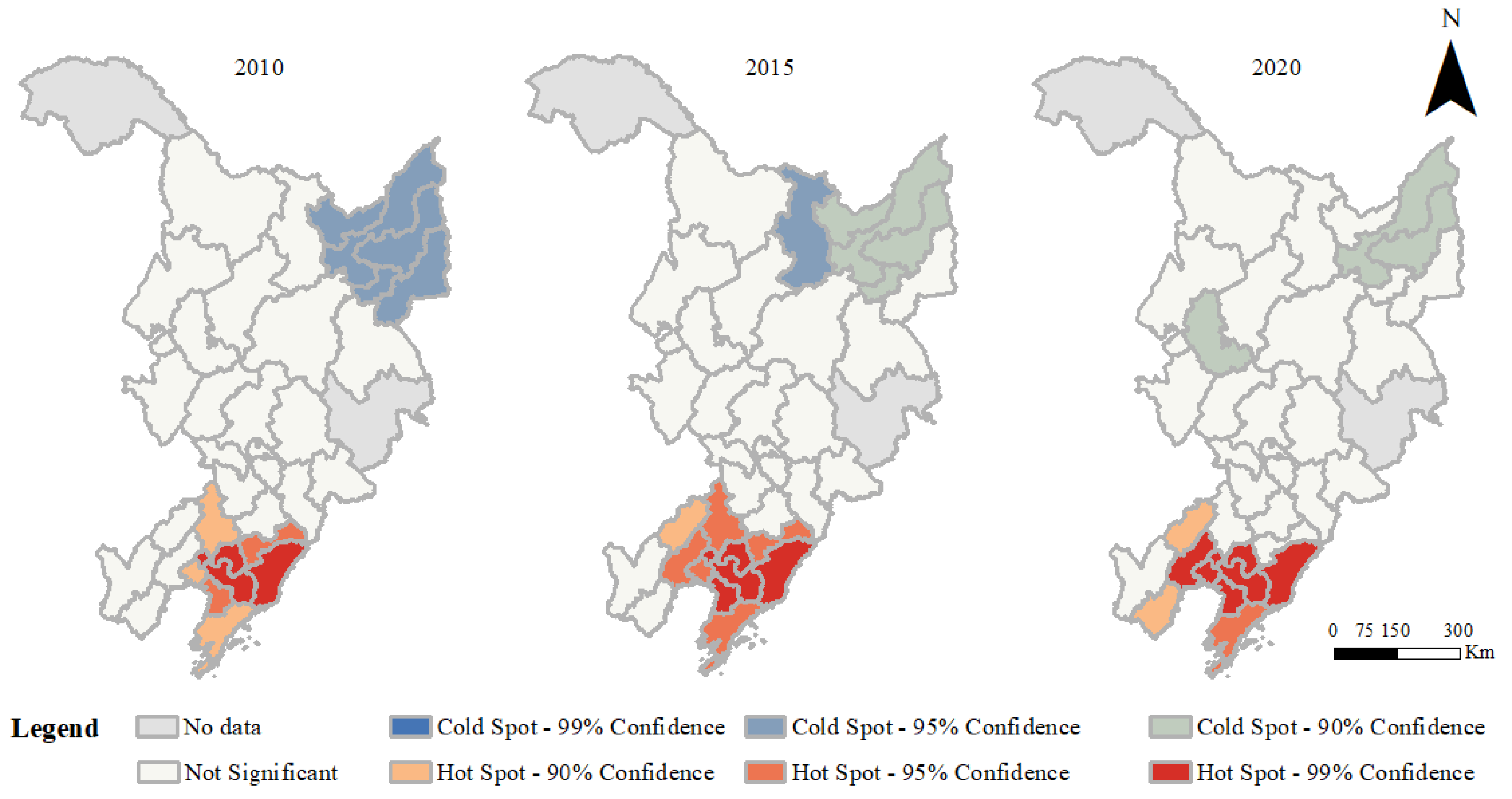
3.3.2. Spatial Characterization Analysis

In order to more intuitively recognize the differences in the spatial distribution of the CCD in the northeast region, ArcGIS was used to visualize the expression (Figure 8), and the Getis-Ord Gi* index was applied to identify further the high-value clustered areas and low-value clustered areas of the coordination level (Figure 9), which were analyzed as follows:

Coordination-level hotspots are concentrated in the Central and Southern Liaoning area, with the cities of Shenyang and Dalian as the core and the surrounding cities of Panjin, Yingkou, Dandong, Anshan, and Liaoyang forming a hotspot of coordination level. The region was composed mostly of cities with non-shrinking populations and mildly shrinking cities, and the level of coordination was generally high. Among them, Shenyang and Dalian showed a “high-high” concentration of Moran’s I in 2010 and 2020, demonstrating that during the research period, the level of coordination in the region has greatly grown, forming a coordination level highland and gradually balanced spatial distribution. However, in 2020, Dandong shifted from a “high-high” to a “low-high” value agglomeration unit, which to a certain extent also reflected the existence of differences within the Central and Southern Liaoning area.

The cold spot area of coordination level is located mainly in northeastern Heilongjiang Province, the region were cities with medium population shrinkage, and the level of coordination was generally low, especially Jiamusi, Shuangyashan, and other areas located at the border, far away from the Harbin-Daqing-Qiqihar industrial corridor, and could hardly reach the scope of influence of the radiation effect. Moreover, this region is mostly for resource cities, the transformation was not thorough enough, the fixed asset investment was insufficient, has not yet formed new industries, and the resource consumption was still serious. As a result, the employment environment was poor, the population loss was serious, and the urbanization and GTFP were low, forming a coordination level “depression” area. However, as can be seen from Figure 9, the scope of the cold spot area has been shrinking during the study period, and the number of “low-low” value agglomeration units has been reduced, indicating that the resource-oriented cities are gradually transforming, merging counties, focusing on ecological development, and improving the level of coordination.

From the spatial dimension, the level of coordination in the northeast region showed a clustered distribution pattern, with significant positive spatial autocorrelation (

Table 8. Moran’s I measured values.

Year	Moran’s I	p-Value	Z-Value
2010	0.051	0.009	2.618
2011	0.033	0.038	2.071
2012	0.034	0.037	2.085
2013	0.097	0.000	4.096
2014	0.100	0.000	4.196
2015	0.070	0.001	3.237
2016	0.080	0.000	3.595
2017	0.017	0.118	1.561
2018	0.065	0.001	3.215
2019	0.037	0.029	2.183
2020	0.051	0.008	2.644

), and all of them were significant at the 0.1% level.

In 2010, the coupling coordination high-value area presented the centralized distribution characteristics centered on Dalian, Shenyang, Changchun, Harbin, and other cities; in 2015, more cities in Heilongjiang Province and Jilin Province transitioned to the coupling coordination high-value area, and the distribution of high-value agglomeration in central and eastern cities of Liaoning was notable; in 2020, with the balance of a higher level of coordination dominating, the coupling coordination of the three provinces of the higher level of cities in successive layouts, presenting a higher level of balance of the layout.

3.4. Analysis of Influencing Factors

3.4.1. Variable Selection and Regression Analysis

The level of coordination is influenced by a number of factors, with reference to the existing studies [28,42], and taking into account the actual situation, the degree of coordination of urbanization and GTFP coupling was taken as the explanatory variable, and the influencing variables were set to be the degree of government intervention, industrial structure, level of external opening, scientific and technological input, knowledge spillover, and environmental regulation (

Table 9. Selection of influencing factor variables.

Category	Variable Name	Variable Symbols	Variable Description	Unit
Explained variables	Coupling coordination	D	Calculation results of the coupling coordination model	/
Explanatory variables	Level of government intervention	gov	Total government spending as a percentage of GDP	%
	Industry structure	ind	Ratio of secondary industry to tertiary industry	%
	Level of external opening	open	Foreign direct investment as a proportion of GDP	%
	Technology input	tec	Science and technology spending as a share of GDP	%
	Knowledge spillover	kno	Share of education technology employees	%
	Environmental regulation	er	Environmental Word Frequency Composite Index	%

).

The above study showed that the distribution of the CCD in the northeast had a certain spatial correlation, indicating that the geospatial element should be taken into account when studying its influencing factor; therefore, the spatial measurement model was chosen. Before the regression, it was first tested jointly by LM (Lagrange multiplier), Robust-LM (robust Lagrange multiplier) as well as Wald, LR (likelihood ratio) index, and Hausman, and, finally, the SDM model under the three kinds of fixed effects of double-fixed, time-fixed, and individual fixed was selected in this study to be fitted and analyzed, and at the same time, the spatial geographic matrix was set up to for robustness testing. The model was set up as follows:

$$Y_{it}=\alpha +{\rho WY}_{it}+{\delta X}_{it}+{\beta WX}_{it}+{\mu }_i+{\phi }_t+{\epsilon }_{it}$$

(11)

where $Y_{it}$ was the explained variable; $X_{it}$ was the explanatory variable; W was the spatial weight matrix; $\alpha$ was the constant term; ${\mu }_i$ and ${\phi }_t$ were individual and time fixed effects; ${\epsilon }_{it}$ was the residual. ${\rho WY}_{it}$ denoted the effect of neighboring regions’ explained variables on local explained variables, and ${\beta WX}_{it}$ denoted the effect of neighboring regions’ explanatory variables on local explanatory variables. To measure the marginal effect of each influencing factor, the total effect was decomposed into direct and indirect effects [43].

3.4.2. Analysis of Influencing Factors

Under the spatial economic distance matrix, Stata 16.0 software was applied to fit the above model (

Table 10. Estimation results of econometric model.

Influencing Factors	CCD of Urbanization and GTFP
	Spatial Economic Distance Matrix			Spatial Geographic Distance Matrix
	Double Fixed	Fixed Time	Individual Fixation	Double Fixed	Fixed Time	Individual Fixation
gov	−0.00593 (−1.36)	−0.0349 *** (−4.16)	−0.00371 (−0.77)	−0.00369 (−0.83)	−0.0605 *** (−6.41)	−0.00520 (−1.13)
ind	0.0106 ** (3.24)	0.00879 * (2.03)	0.00534 (1.57)	0.0140 *** (3.96)	0.0158 ** (2.70)	0.00857 ** (2.59)
open	0.00446 (0.15)	0.144 * (2.35)	−0.000652 (−0.02)	−0.00203 (−0.07)	0.237 *** (3.41)	0.00727 (0.23)
tec	0.362 (0.47)	5.864 *** (4.56)	−0.463 (−0.55)	0.151 (0.19)	6.988 *** (4.35)	0.128 (0.16)
kno	0.0630 (0.76)	−0.310 *** (−4.71)	0.0336 (0.37)	0.102 (1.24)	−0.605 *** (−7.38)	0.0839 (0.97)
er	1.229 (1.18)	−3.885 * (−2.24)	1.967 (1.74)	2.264 * (2.03)	−8.474 *** (−3.95)	1.854 (1.69)
WX	Yes	Yes	Yes	Yes	Yes	No
Coefficient	−0.165 (−1.62)	0.442 *** (5.82)	0.719 *** (19.47)	−0.285 (−1.31)	0.110 (0.61)	0.840 *** (25.12)
R2	0.0454	0.0467	0.0231	0.00397	0.0480	0.0231
Sigma2	0.000417 *** (13.65)	0.00192 *** (13.33)	0.000520 *** (13.41)	0.000427 *** (13.65)	0.00263 *** (13.65)	0.000474 *** (13.51)
Log-L	923.9074	635.7808	863.4688	919.7746	580.5328	887.2716

Note: The t-values are reported in parentheses. * p < 0.05, ** p < 0.01, *** p < 0.001.

). The coordination level of urbanization and GTFP had a higher fit R² under the time-fixed model than that of the double fixed-effects and individual fixed-effects models, and the study data were long time series panel data (T > N), so the spatial Durbin model under the time-fixed effect was selected for the explanatory analysis, and the results were as follows:

The degree of government intervention (−0.0349) and the intensity of environmental regulation (−3.885) negatively and significantly affected the coordination level of urbanization and GTFP (hereinafter referred to as the coordination level). Science and technology investment (5.864) positively and significantly affected the coordination level, and the degree of knowledge spillover (−0.310) negatively and significantly affected the coordination level, i.e., in the study period, as the proportion of science and technology expenditures increased, the coordination level tended to increase; the higher the percentage of people pursuing education in science and technology, the lower the coordination level. The industrial structure (0.00879) and the level of openness to the outside world (0.144) significantly and positively affected the coordination level.

3.4.3. Spatial Spillovers of Influencing Factors

The total effect was decomposed through a partial differential equation to explore better the direct and spillover effects of the influencing factors on the coordinated level (

Table 11. Decomposition of spatial effect.

Influencing Factors	CCD of Urbanization and GTFP
	Spatial Economic Distance Matrix			Spatial Geographic Distance Matrix
	Direct Effect	Indirect Effect	Total Effect	Direct Effect	Indirect Effect	Total Effect
gov	−0.0389 *** (−4.38)	−0.0891 (−1.93)	−0.128 ** (−2.59)	−0.0606 *** (−6.20)	−0.0909 (−0.91)	−0.152 (−1.48)
ind	0.0212 *** (3.96)	0.258 *** (5.44)	0.279 *** (5.47)	0.0165 ** (2.79)	0.164 * (2.57)	0.180 ** (2.70)
open	0.197 ** (2.92)	0.968 * (2.25)	1.165 * (2.47)	0.253 *** (3.72)	1.734 * (2.39)	1.987 ** (2.70)
tec	6.467 *** (4.74)	13.85 * (2.08)	20.32 ** (2.76)	6.843 *** (4.26)	−12.70 (−0.81)	−5.856 (−0.36)
kno	−0.349 *** (−5.38)	−0.805 * (−2.53)	−1.154 *** (−3.43)	−0.598 *** (−7.23)	1.528 * (2.17)	0.930 (1.29)
er	−4.471 * (−2.51)	−13.02 (−1.39)	−17.49 (−1.73)	−8.630 *** (−4.01)	−34.63 (−1.42)	−43.26 (−1.71)

Note: The t-values are reported in parentheses. * p < 0.05, ** p < 0.01, *** p < 0.001.

).

As local government behaviors, both government intervention and environmental regulation only had significant direct effects on the local area, i.e., for every 1% increase in the degree of government intervention, the local coordination level decreased by 0.0389%; local coordination fell by 4.471% for every 1% rise in the amount of environmental regulation. Moderate government intervention and environmental regulation could help improve the coordination level, so the governments of prefecture-level cities should build a communication and coordination mechanism between new urbanization and green development and cooperate in infrastructure, health care, and environmental governance. Policy instruments such as carbon emissions trading schemes [44], for example, have been adopted to ban straw burning in the northeast and to enhance the development of green infrastructure networks [45,46]. Industrial structure, openness to the outside world, scientific and technological investment, and knowledge spillover not only had direct effects on the local area, but also had spillover effects on the neighboring areas. Industrial structure, opening-up level, and scientific and technological input were positive effects, and knowledge overflow was negative. This indicated that there existed the phenomenon of agglomeration between cities and the formation of city clusters for synergistic development. This could be reflected in a gradual increase in the agglomeration of cities with high similarity, especially in and around the central cities, which allocated more resources and were more efficiently implemented [47].

3.4.4. Heterogeneity Analysis of Influencing Factors

The regression results indicated that government intervention, industrial structure, openness level, scientific and technological investment, knowledge spillover, and environmental regulation had significant positive effects on all shrinking degree cities under the total effect (

Table 12. Analysis of heterogeneity among cities with different degrees of shrinkage.

	CCD of Urbanization and GTFP
	Non-Shrinking Cities	Mildly Shrinking Cities	Moderately Shrinking Cities	Severely Shrinking Cities
gov	−0.094 (0.229)	0.050 ** (0.017)	−0.005 (0.004)	−0.115 *** (0.010)
ind	−0.036 (0.020)	0.016 *** (0.004)	−0.000 (0.011)	−0.129 ** (0.026)
open	−0.039 (0.028)	0.018 (0.178)	0.004 (0.028)	0.561 *** (0.018)
tec	3.221 (3.045)	−8.920 ** (3.236)	0.567 (1.214)	−3.343 *** (0.118)
kno	0.008 (0.163)	−0.057 (0.176)	0.218 (0.170)	−0.863 (0.613)
er	−5.180 (2.328)	−1.243 (2.350)	2.521 (1.863)	0.100 (6.068)
_cons	0.949 *** (0.050)	0.749 *** (0.023)	0.694 *** (0.012)	1.032 *** (0.148)
N	33.000	99.000	209.000	33.000
R2	0.933	0.612	0.691	0.861

Note: Standard errors in parentheses. ** p < 0.05, *** p < 0.01.

), and the effects were more significant for the severely shrinking cities. Among the government factors, the degree of government intervention only had a significant positive effect on the mildly shrinking (0.050) cities, had a negative effect on the non-shrinking (−0.094) and moderately shrinking (−0.005) cities, but not significant, and had a significant negative effect on the severely shrinking (−0.115) cities, suggesting that the government’s over-intervention would instead cause redundancy of resources and form unnecessary waste. As population shrinkage deepened, environmental regulations gradually shifted from a negative to a positive effect, but not significantly. That was attributed to the fact that environmental regulation contributed to the elimination of the curse effect of political relations on technological innovation by increasing market competition and reducing overinvestment [28]. In the northeast, the market system is rigid, the state-owned enterprises are not competitive, and a certain amount of fixed investment of the state financial transfer is occupied. Therefore, the government should intervene to adjust and optimize market institutions.

Among the technological factors, S&T inputs and knowledge spillovers had positive effects in the non-shrinking (3.221, 0.008) and moderately shrinking (0.567, 0.218) cities, while the opposite was true for the mildly shrinking (−8.920, −0.057) and severely shrinking (−3.343, −0.863) cities. Most of the mildly shrinking cities were around the non-shrinking cities, and due to the “rebound effect,” technological research and development was concentrated in the core cities, which increased production efficiency while expanding their resource demand, at a cost greater than the reduced energy consumption of technological upgrading. Severely shrinking cities, on the other hand, were in the middle of the primary-middle level of coordination, where the existing infrastructure could not meet the needs of science and technology, thus reducing the level of coordination.

Among the economic factors, the industrial structure had significant positive effects in mildly shrinking (0.016) cities, negative effects in non-shrinking (−0.094) and severely shrinking (−0.129) cities, and more significant in severely shrinking cities. The level of openness to the outside world has different effects in shrinking and non-shrinking cities; in non-shrinking (−0.039) cities, the level of openness to the outside world plays a negative role but is not significant. The opposite was true in shrinking cities, and the positive effect was more significant in severely shrinking (0.561) cities. This showed that while population agglomeration was a requirement for social and economic progress, going above the population’s carrying capacity would result in overproduction and the contamination of living things. Industrialization was also shown to have a significant positive impact on economic growth. Severely shrinking cities declined in industry and became the excess capacity of the “supply-side” structural reform, and the demand of the external market was shrinking, resulting in a serious loss of labor and resource depletion, making it difficult to sustain green development. The coordination level of mildly shrinking cities was slightly lower than that of non-shrinking cities; due to the siphoning effect, the population flowed to the core cities of the urban agglomerations and was influenced by the radiation of the core cities, and the relationship between per capita possession of resources and consumption was eased. Moreover, the improvement of the coordination level was facilitated by the industrial structure modification and an acceptable degree of opening up.

4. Discussion

4.1. Population Shrinkage Analysis

From 2010 to 2020, only Changchun, Shenyang, and Dalian did not experience population shrinkage, while the remaining 31 cities suffered different degrees of population shrinkage and used a “high in the north with a low in the south” geographical pattern. The main reasons are as follows. (1) The internal logic of the shrinkage was the weakening of the “development potential” of the region caused by the downturn of the investment and consumption economy [48]. Under the long-term effect of “deindustrialization, suburbanization, globalization” and other factors [49], the economic vitality of Northeast China had declined, and the population showed a gradual shrinkage, i.e., the inflow of population was less than the outflow of population, and the outflow of population were mostly young and middle-aged laborers, which indirectly led to a decline in the birth rate in the region and the rise of the aging population. The shrinkage in general showed a relatively stable inertia and persistent development characteristics. (2) The region had a high degree of primacy, with the economy and resources concentrated in the core city. Under the “polarization” effect, the surrounding population concentrated toward the center, and thus the population was in relative dynamic balance, while its surrounding cities were deprived of space by the central city, and the phenomenon of shrinkage occurred to varying degrees. (3) Population shrinkage cities mostly for resource cities, decline-type resource cities were mainly concentrated in the north of Heilongjiang, such as Yichun, Hegang, and other areas, which were located in the border, access was not high, the depletion of resources led to a severe employment environment, resulting in a large number of population outflow. Regeneration-type resource cities were concentrated mainly in the south of Liaoning, such as Huludao and Panjin, with locational advantages, and were port cities; the marine economy had a certain support for its development and was still in the stage of mild shrinkage.

4.2. Analysis of the Level of Coordination between Urbanization and GTFP

Overall, it showed a circle structure with Harbin-Daqing-Changchun, Shenyang-Dalian as the core and decreasing to the periphery, which was in line with the overall development pattern of Northeast China, i.e., spatial agglomeration along the Harbin-Dalian corridor and from north to south: The “core circle” of Harbin, Changchun, Shenyang, Dalian was the leading economic region in the northeast, but also an advanced demonstration area for urban transformation, with a significant urbanization and GTFP coordination level. Shuangyashan, Chaoyang, Heihe, and Yichun in the “outer circle” had the highest growth rate of coupling coordination level. These areas were mostly ecologically sensitive or geopolitically sensitive areas with less ecological and environmental pressure. Under the influence of national ecological functional areas and other policies, the transformation of urban green development was quite effective. This indicated that the region has been still agglomerating with the urban agglomerations of Harbin-Changchun urban agglomeration and Central and Southern Liaoning area as the core, while inter-regional development tended to be balanced and was experiencing the process of transitioning from a higher level of agglomerations to a higher level of balanced development.

4.3. Analysis of Influencing Factors

The degree of government intervention mainly affected the level of coordination through infrastructure construction. Moderate investment and infrastructure construction were conducive to the development of urbanization and the creation of a green environment, thus increasing GTFP, but excessive infrastructure construction would cause a waste of resources, resulting in a decline in GTFP. Meanwhile, moderate environmental regulation played the leading role of the government, prompting enterprises to technological innovation, and the resulting benefits could compensate for the cost of regulation, realizing a positive cycle, and the green environment was conducive to the development of urbanization. However, excessive environmental regulation would drive up resource costs, and in the interaction between the government and the enterprises, the enterprises might compress the research and development expenditures and investment in innovation, which would hurt the GTFP. Scientific and technological investment for the city to create an innovative environment, technological innovation to promote the green development of enterprises, good technical facilities to attract talent, so that the overall level of R & D, however, due to the current mismatch of resources and other reasons, resulting in knowledge spillover yet to coordinate the level of negative impact. With the transformation of pollution-intensive industries, enterprise production energy consumption decreased, reducing environmental pollution, and opening to the outside world was conducive to stimulating market potential, accelerating the flow of factor resources, stimulating market vitality, and promoting green development.

The reduction of pollution-aggregating enterprises is necessary for dealing with the issue of environmental pollution in the current agglomeration of resource cities. Second, an increase of the degree of exposure to the global outside to draw in human and technological capital. In addition, acceleration of the flow of factor resources and acceleration of industrial structure upgrading and green transformation, so as to positively influence the level of coordination in both urbanization and green development. Therefore, local governments ought to, on the one hand, actively promote scientific and technical investment, innovate technology, increase energy efficiency and decrease resource consumption. On the other hand, they should deepen the convergence of industrial planning and the connection between them of industrial structure. In addition, they should coordinate the knowledge spillover with the allocation of resource factors to realize the transformation, so that intellectual capital can be used as a reserve of talents to build up the strength for improving innovative technologies and to enhance the whole level of research.

5. Conclusions

This research concentrated on the two key themes of urbanization and ecology by taking the cities in the “Rust Belt” of China as samples to empirically analyze the spatial and temporal evolution of the coupling and coordination of urbanization and GTFP in 34 cities, and quantitatively analyzing the key influencing factors, to investigate the coordinated creation of high-quality urban transformation and GTFP within the context of population shrinkage and to come up with the following conclusions.

The population of the three northeastern provinces as a whole has shown a trend of shrinkage, characterized by a spatial pattern of “high in the north and low in the south.” The level of urbanization and GTFP were on the rise, spatially showing a “core-edge” pattern centered on Harbin-Changchun, Shenyang-Dalian, and spreading in all directions. The urbanization level of non-shrinking cities was much higher than that of shrinking cities. In shrinking cities, the coordination level continued to decline as the degree of shrinkage increased. The overall difference in GTFP was relatively slight, with mildly shrinking and moderately shrinking cities experiencing relatively smooth changes, and non-shrinking and severely shrinking cities experiencing larger changes, exhibiting a general growing pattern.

The coordination level of urbanization and GTFP presented the characteristics of the transition from “primary coordination” to “intermediate coordination.” In terms of spatial pattern, it showed a circle structure with Harbin-Daqing-Changchun, and Shenyang-Dalian as the core and decreasing to the periphery. The coordination level of cities with a non-shrinking population was significantly higher than that of cities with a shrinking population. In shrinking cities, as the degree of shrinkage increased, the level of coordination continued to decline, and regional differences gradually narrowed, forming a balanced development trend. The level of coordination was affected by government factors, technical factors, and economic factors. Among them, government intervention, environmental regulation, and knowledge spillover had negative effects on the coordination level, while beneficial effects on the industrial structure, external access, and technological investment created spatial spillover effects.

The influencing factors of coordination level showed certain regional heterogeneity. Under the total effect, the influencing factors had a significant positive effect on cities with all degrees of shrinkage, and the effect on cities with severe shrinkage was more significant. Government intervention and industrial structure only had a significant positive effect on mildly shrinking cities. As the degree of shrinkage deepened, the effects of the level of opening up and environmental regulation on the level of coordination gradually changed from negative correlation to positive correlation; technology investment and knowledge spillover had a positive impact in non-shrinking and moderately shrinking cities and a negative impact in mildly and severely shrinking cities on the coordination level.

In response to the above discussion, in the future, Northeast China may seek new points of focus for coordinated development in the midst of shrinkage. First, it is important to pay attention to the phenomenon of population shrinkage and to look at its impacts in a dialectical manner. The government should stabilize the population, recognize the fact of shrinkage, reevaluate and position the city types, guide them in a categorical manner, reconstruct the development space of the stock, promote the moderate migration of the population, improve the public service and pension system, and increase the population’s desire for staying in the city. It will improve the quality of the population, perfect the household registration system and social security system, upgrade the level of medical care, health care, education, and public facilities, and promote policies on housing security and the introduction of talent, in order to encourage the coordinated growth of urban assets and people. Second, to achieve the green transformation of the northeast region, it must integrate urbanization with the establishment of ecological civilization within the context of population reduction and overcome the route dependence of regional development and strengthen the northeast region’s integrated development. In addition, it should adopt differentiated strategies within the region, optimize and adjust the industrial structure, integrate production factors, develop low-carbon innovative economic models, optimize the spatial spillover effect, and give play to the driving role of the pioneer demonstration areas to radiate the surrounding cities. Mildly shrinking cities with a certain industrial foundation strengthen the construction of regional industrial chains, absorb the technology and resources of core cities, and clarify the industrial division of labor and upgrading. Border areas focus on the combination of economic development and ecological environmental protection, rely on high-quality natural background and product advantages, strengthen cooperation with neighboring countries and regions, promote the transformation of resource-oriented cities, and realize diversified development.

In addition, urban development is a comprehensive result of the complex interaction of many factors. Due to the availability of data, this paper did not include the housing vacancy rate, the quality of the demographic structure, and so on. There is still room for optimization in the construction of research indicators and models, so it fails to specifically quantify the relationship between population shrinkage and the economic society and the ecological environment. These deficiencies will be the focus of the next study.

References

1. UN. 2018 Revision of World Urbanization Prospects. 2018. Available online: https://www.un.org/zh/desa/2018-revision-world-urbanization-prospects (accessed on 13 April 2023).
2. Fan, J.J.; Wang, J.L.; Qiu, J.X.; Li, N. Stage effects of energy consumption and carbon emissions in the process of urbanization: Evidence from 30 provinces in China. Energy 2023, 276, 127655. [Google Scholar] [CrossRef]
3. Wang, J.Y.; Wang, S.J.; Li, S.J.; Feng, K.S. Coupling analysis of urbanization and energy environment efficiency: Evidence from Guangdong province. Appl. Energy 2019, 254, 113650. [Google Scholar] [CrossRef]
4. Bi, Y.Z.; Zheng, L.; Wang, Y.; Li, J.F.; Yang, H.; Zhang, B.W. Coupling relationship between urbanization and water-related ecosystem services in China’s Yangtze River economic Belt and its socio-ecological driving forces: A county-level perspective. Ecol. Ind. 2023, 146, 109871. [Google Scholar] [CrossRef]
5. Shi, X.Y.; Matsui, T.; Machimura, T.; Haga, C.; Hu, A.; Gan, X.Y. Impact of urbanization on the food–water–land–ecosystem nexus: A study of Shenzhen, China. Sci. Total Environ. 2022, 808, 152138. [Google Scholar] [CrossRef]
6. Huang, Z.Y.; An, X.Y.; Cai, X.R.; Chen, Y.N.; Liang, Y.Q.; Hu, S.X.; Wang, H. The impact of new urbanization on PM2.5 concentration based on spatial spillover effects: Evidence from 283 cities in China. Sustain. Cities Soc. 2023, 90, 104386. [Google Scholar] [CrossRef]
7. Xu, J.J.; Wang, J.C.; Li, R.; Yang, X.J. Spatio-temporal effects of urbanization on CO2 emissions: Evidences from 268 Chinese cities. Energy Policy 2023, 177, 113569. [Google Scholar] [CrossRef]
8. Liu, R.R.; Dong, X.B.; Wang, X.C.; Zhang, P.; Liu, M.X.; Zhang, Y. Relationship and driving factors between urbanization and natural ecosystem health in China. Ecol. Ind. 2023, 147, 109972. [Google Scholar] [CrossRef]
9. Weiskopf, S.R.; Rubenstein, M.A.; Crozier, L.G.; Gaichas, S.; Griffis, R.; Halofsky, E.J.; Hyde, K.J.W.; Morelli, T.L.; Morisette, J.T.; Muñoz, R.C. Climate change effects on biodiversity, ecosystems, ecosystem services, and natural resource management in the United States. Sci. Total Environ. 2020, 733, 137782. [Google Scholar] [CrossRef] [PubMed]
10. Crandall, R.W. The Continuing Decline of Manufacturing in the Rust Belt; Brookings Institution: Washington, DC, USA, 1993. [Google Scholar]
11. Hobor, G. Surviving the era of deindustrialization: The new economic geography of the urban rust belt. J. Urban Aff. 2013, 35, 417–434. [Google Scholar] [CrossRef]
12. Xie, L.; Yang, Z.S.; Cai, J.M.; Cheng, Z.; Wen, T.; Song, T. Harbin: A rust belt city revival from its strategic position. Cities 2016, 58, 26–38. [Google Scholar] [CrossRef]
13. National Bureau of Statistics. 2006–2020. Available online: http://www.stats.gov.cn/ (accessed on 13 April 2023).
14. Wu, X.Y.; Zhang, Y.J.; Wang, L.Z. Coupling relationship between regional urban development and eco-environment: Inspiration from the old industrial base in Northeast China. Ecol. Ind. 2022, 142, 109259. [Google Scholar] [CrossRef]
15. Caviglia-Harris, J.L.; Chambers, D.; Kahn, J.R. Taking the “U” out of Kuznets: A comprehensive analysis of the EKC and environmental degradation. Ecol. Econ. 2009, 68, 1149–1159. [Google Scholar] [CrossRef]
16. Kuznets, S. Economic growth and income equality. Am. Econ. Rev. 1955, 45, 1–28. [Google Scholar]
17. OECD. Indicators to Measure Decoupling of Environmental Pressure from Economic Growth; OECD: Paris, France, 2022. [Google Scholar]
18. Ma, S.J.; Wang, R.S. The social-economical-natural complex ecosystem. Acta Ecol. Sin. 1984, 4, 1–9. [Google Scholar]
19. Fang, C.L.; Zhou, C.H.; Gu, C.L.; Chen, L.D.; Li, S.C. Theoretical analysis of interactive coupled effects between urbanization and eco-environment in mega-urban agglomerations. Acta Geogr. Sin. 2016, 71, 531–550. [Google Scholar] [CrossRef]
20. Fang, C.L.; Cui, X.G.; Liang, L.W. Theoretical analysis of urbanization and eco-environment coupling coil and coupler control. Acta Geogr. Sin. 2019, 74, 2529–2546. [Google Scholar]
21. Wei, G.E.; Bi, M.; Liu, X.; Zhang, Z.K.; He, B.J. Investigating the impact of multi-dimensional urbanization and FDI on carbon emissions in the belt and road initiative region: Direct and spillover effects. J. Clean. Prod. 2022, 384, 135608. [Google Scholar] [CrossRef]
22. Wang, W.Z.; Liu, L.C.; Liao, H.; Wei, Y.M. Impacts of urbanization on carbon emissions: An empirical analysis from OECD countries. Energy Policy 2021, 151, 112171. [Google Scholar] [CrossRef]
23. Warsame, A.A.; Abdi, A.H.; Amir, A.Y.; Azman-Saini, W.N.W. Towards sustainable environment in Somalia: The role of conflicts, urbanization, and globalization on environmental degradation and emissions. J. Clean. Prod. 2023, 406, 136856. [Google Scholar] [CrossRef]
24. Ahmed, Z.; Zafar, M.W.; Ali, S. Linking urbanization, human capital, and the ecological footprint in G7 countries: An empirical analysis. Sustain. Cities Soc. 2020, 55, 102064. [Google Scholar] [CrossRef]
25. Feng, Y.D.; Yuan, H.X.; Liu, Y.B. The energy-saving effect in the new transformation of urbanization. Econ. Anal. Policy 2023, 78, 41–59. [Google Scholar] [CrossRef]
26. Yao, Y.R.; Shen, Y.; Liu, K.X. Investigation of resource utilization in urbanization development: An analysis based on the current situation of carbon emissions in China. Resour. Policy 2023, 82, 103442. [Google Scholar] [CrossRef]
27. Levin, S.; Xepapadeas, T.; Cr’epin, A.-S.; Norberg, J.; Zeeuw, A.D.; Folke, C.; Hughes, T.; Arrow, K.; Barrett, S.; Daily, G. Social-ecological systems as complex adaptive systems: Modeling and policy implications. Environ. Dev. Econ. 2013, 18, 111–132. [Google Scholar] [CrossRef]
28. Gao, D.; Li, Y.; Tan, L.F. Can environmental regulation break the political resource curse: Evidence from heavy polluting private listed companies in China. J. Environ. Plan. Manag. 2023, 1–27. [Google Scholar] [CrossRef]
29. Diao, S.; Yuan, J.D. Multidimensional measurements of coordinated development level of Harbin-Changchun urban agglomeration. Econ. Geogr. 2022, 42, 86–94. [Google Scholar]
30. Sun, Y.S.; Tong, L.J. Spatio-temporal coupling relationship between development strength and eco-environment in the restricted development zone of Northeast China. Sci. Geogr. Sin. 2021, 41, 684–694. [Google Scholar]
31. Zhao, J.J.; Liu, Y.; Zhu, Y.K.; Qin, S.L.; Wang, Y.H.; Miao, C.H. Spatiotemporal differentiation and influencing factors of the coupling and coordinated development of new urbanization and ecological environment in the Yellow River Basin. Resour. Sci. 2020, 42, 159–171. [Google Scholar] [CrossRef]
32. Ostrom, E. A general framework for analyzing sustainability of social-ecological systems. Science 2009, 325, 419–422. [Google Scholar] [CrossRef]
33. Xu, Z.H.; Peng, J.; Liu, Y.X.; Qiu, S.J.; Zhang, H.B.; Dong, J.Q. Exploring the combined impact of ecosystem services and urbanization on SDGs realization. Appl. Geogr. 2023, 153, 102907. [Google Scholar] [CrossRef]
34. Liu, Z.; Qi, W.; Qi, H.G.; Liu, S.H. The evolution of regional population decline and its driving factors at the county level in China from 1990 to 2015. Geogr. Res. 2020, 39, 1565–1579. [Google Scholar]
35. Qi, W.; Liu, S.H.; Jin, F.J. Calculation and spatial evolution of population loss in Northeast China. Sci. Geogr. Sin. 2017, 37, 1795–1804. [Google Scholar]
36. Li, H.; Liang, X.X. Responses of housing price under different directions of population change: Evidence from China’s Rust Belt. Chin. Geogr. Sci. 2022, 32, 405–417. [Google Scholar] [CrossRef]
37. Ning, J. Main Data of the Seventh National Population Census From. 2021. Available online: http://www.stats.gov.cn/english/PressRelease/202105/t20210510_1817185.html (accessed on 13 April 2023).
38. Liu, Z.; Qi, H.G.; Qi, W.; Liu, S.H. Temporal- spatial pattern of regional population shrinkage in China in 1990–2010: A multi-indicators measurement. Sci. Geogr. Sin. 2019, 39, 1525–1536. [Google Scholar]
39. Fu, J.Y.; Hu, J.; Cao, X. Different sources of FDI, environmental regulation and green total factor productivity. J. Int. Trade 2018, 7, 134–148. [Google Scholar]
40. Wang, S.J.; Kong, W.; Ren, L.; Zhi, D.D.; Dai, B.T. Research on misuses and modification of coupling coordination degree model in China. J. Nat. Resour. 2021, 36, 793–810. [Google Scholar] [CrossRef]
41. Wolff, M.; Wiechmann, T. Urban growth and decline: Europe’s shrinking cities in a comparative perspective 1990—2010. Eur. Urban Reg. Stud. 2018, 25, 122–193. [Google Scholar] [CrossRef]
42. Zhang, K.Y.; Zhang, J. Polycentricity and green development efficiency of urban agglomerations: Spatial distribution of urbanization based on heterogeneity. China Popul. Resour. Environ. 2022, 32, 107–117. [Google Scholar]
43. Zhu, W.T.; Lv, C.R.; Gu, N.H. Research on the influence of OFDI and reverse technology spillover on green total factor productivity. China Popul. Resour. Environ. 2019, 29, 63–73. [Google Scholar]
44. Gao, D.; Tan, L.; Mo, X.; Xiong, R. Blue Sky Defense for Carbon Emission Trading Policies: A Perspective on the Spatial Spillover Effects of Total Factor Carbon Efficiency. Systems 2023, 11, 382. [Google Scholar] [CrossRef]
45. Yang, G.Y.; Zhao, H.M.; Tong, D.Q.; Xiu, A.J.; Zhang, X.L.; Gao, C. Impacts of post-harvest open biomass burning and burning ban policy on severe haze in the Northeastern China. Sci. Total Environ. 2020, 716, 136517. [Google Scholar] [CrossRef]
46. Bai, Y.J.; Guo, R. The construction of green infrastructure network in the perspectives of ecosystem services and ecological sensitivity: The case of Harbin, China. Glob. Ecol. Conserv. 2021, 27, e01534. [Google Scholar] [CrossRef]
47. Chen, Y.; Zhang, D.N. Evaluation and driving factors of city sustainability in Northeast China: An analysis based on interaction among multiple indicators. Sustain. Cities Soc. 2021, 67, 102721. [Google Scholar] [CrossRef]
48. Sun, P.J.; Wang, K.W. Identification and stage division of urban shrinkage in the three provinces of Northeast China. Acta Geogr. Sin. 2021, 76, 1366–1379. [Google Scholar]
49. Batty, M. Empty buildings, shrinking cities and ghost towns. Environ. Plan. B Plan. Des. 2016, 43, 3–6. [Google Scholar] [CrossRef]
Figure 1. Northeast China’s location in the world.
Sustainability 16 01312 g001
Figure 2. Spatial distribution of population shrinkage in Northeast China.
Sustainability 16 01312 g002
Figure 3. Spatial distribution of urbanization level in 2010–2020.
Sustainability 16 01312 g003
Figure 4. Spatial distribution of GTFP in 2010–2020.
Sustainability 16 01312 g004
Figure 5. Measurement of urbanization levels in cities with different degrees of shrinkage.
Sustainability 16 01312 g005
Figure 6. Measurement of GTFP in cities with different degrees of shrinkage.
Sustainability 16 01312 g006
Figure 7. Changes in CCD of cities with different degrees of shrinkage from 2010 to 2020.
Sustainability 16 01312 g007
Figure 8. Spatial pattern changes of CCD from 2010 to 2020.
Sustainability 16 01312 g008
Figure 9. Hotspot analysis of the CCD.
Sustainability 16 01312 g009