Evolution of China’s Coastal Economy since the Belt and Road Initiative Based on Nighttime Light Imagery

Abstract

The joint construction of the Silk Road Economic Belt and the 21st Century Maritime Silk Road proposed by China has brought major development opportunities for the development of countries and regions along the routes. Traditional GDP statistics based on administrative units cannot describe the spatial differences of GDP within administrative units, which has certain limitations in exploring regional economic development analysis and supporting economic development decision making. Based on NPP-VIIRS luminous remote sensing data, land use data, and statistical yearbook data, this paper analyzes the spatial–temporal evolution pattern of economic level in China’s coastal economic belt from 2012 to 2021 using the Moran index and standard deviation ellipse. An unbalanced distribution of economic development are found along China coastal area and the economic gravity center moved southwest since the Belt and Road Initiative. The results show thatthe Yangtze River Delta was extremely active , and the economic growth of the south was better than that of the north. The grided GDP map presents more details of regional economic development, and provides an opportunity for further mechanisms exploration of the development process.

1. Introduction

In 2013, Chinese President Xi Jinping first proposed the Belt and Road Initiative (BRI) [1,2,3]. In the 10 years since its launch, 151 countries and 32 international organizations have signed BRI cooperation documents with China. The National Development and Reform Commission of the People’s Republic of China and relevant departments jointly issued the Vision and Action on Jointly Building the Silk Road Economic Belt and the 21st Century Maritime Silk Road, pointing out that China’s coastal cities should be the core of the construction of the Maritime Silk Road. In the spirit of enhancing pragmatic cooperation with countries along the Road, the Chinese government has encouraged economic zones such as the Bohai Rim, the Yangtze River Delta, the Pearl River Delta, and coastal port cities [4]. The coastal economic belt has become the most developed and concentrated area of urban agglomerations in China, so it is of great research significance and important application value to explore its economic development and evolution pattern.

Nighttime light (NTL) remote sensing is an optical remote sensing technology that can detect night light. The earliest NTL observation began in the 1970s with the U.S. Defense Meteorological Satellite Program (DMSP), which opened the era of NTL remote sensing image application [5]. Since the DMSP-OLS digital archiving of NTL remote sensing data by NOAA National Geophysical Data Center for the first time in 1992 [5], DMSP-OLS has been widely used in various regional development assessment and simulation studies at different scales. Shi et al. [6] proposed panel data analysis to model spatiotemporal CO₂ emission dynamics in China from DMSP-OLS nighttime stable light data. Bustos and Hall [7] used DMSP data to fit demographic data to derive demographic changes in Europe between 1992 and 2012. Zhou et al. [8] showed the potential to map global urban extent and temporal dynamics using the DMSP/OLS NTL data in a timely, cost-effective way with a cluster-based method. Nevertheless, the DMSP-OLS effective application is limited by its sensor technology, which has obvious defects, such as rough radiation measurement accuracy, low spatial resolution, and lack of spaceborne calibration [5,9]. In 2012, the Visible Infrared Imaging Radiometer Suite (VIIRS) onboard the Suomi National Polar Partnership (NPP) provided a new generation of NTL data, representing a milestone revolution of NTL. Since NPP-VIIRS data overcome the main defects of DMSP-OLS data, the NTL remote sensing data can be used to study socioeconomic problems in a higher spatial resolution [10,11,12]. Chen et al. [11] calculated the county-level carbon sequestration value of terrestrial vegetation in China from 1997 to 2017 with NPP/VIIRS satellite imagery. Li et al. [13] estimated electric load density at a township-level spatial scale based on NPP/VIIRS night light satellite data. Zhou et al. [14] estimated city-level CO₂ combined NPP/VIIRS data with socioeconomic data. The above studies indicate that NPP-VIIRS can serve as a reliable proxy for the assessment of social, economic, and environmental indicators at different scales.

Socioeconomic indicators such as gross national product (GDP) are a comprehensive and quantitative description of the socioeconomic development of a country or region. Since NTL data can make up for the significant defects of traditional statistical data, such as inconsistent statistical standards, missing data, and low updating frequency, it provides the possibility for spatial distribution of economic indicators and fine evaluation of economic activities [15,16,17]. The NTL data have been proved by many studies to have a strong correlation with GDP, poverty, carbon emissions, electricity consumption, urban population, housing vacancy rate, freight volume, and other social and economic indicators. As early as 1997, Elvidge et al. [5] used DMSP data to regress the GDP data and night light area of American countries and found that the goodness of fit between the two was as high as 0.97 at the national scale. Since then, a large number of studies have used night light remote sensing data to estimate GDP at the national scale [18], provincial scale [16], and grid scale [19]. Li et al. [20] analyzed 31 provincial regions and 393 county regions in China and found that the NPP/VIIRS data performed better than DMSP-OLS in predicting GDP. However, due to the neglect of the low correlation between the primary industry and the NTL remote sensing index, the spatial model overestimates the low-productivity areas [21]. Therefore, it is often more feasible to decompose GDP into agriculture and non-agriculture and then model its total GDP spatial distribution respectively [22]. The aims of this paper are (1) using annual synthesis and seasonal mask denoising (SMD) methods to obtain denoised annual composite NPP-VIIRS NTL data; (2) building pixel-level estimation models for GDP and spatializing the indicator on a 1 km resolution grid; and (3) analyzing the spatiotemporal dynamics of GDP at multiple scales and perspectives.

2. Materials and Methods

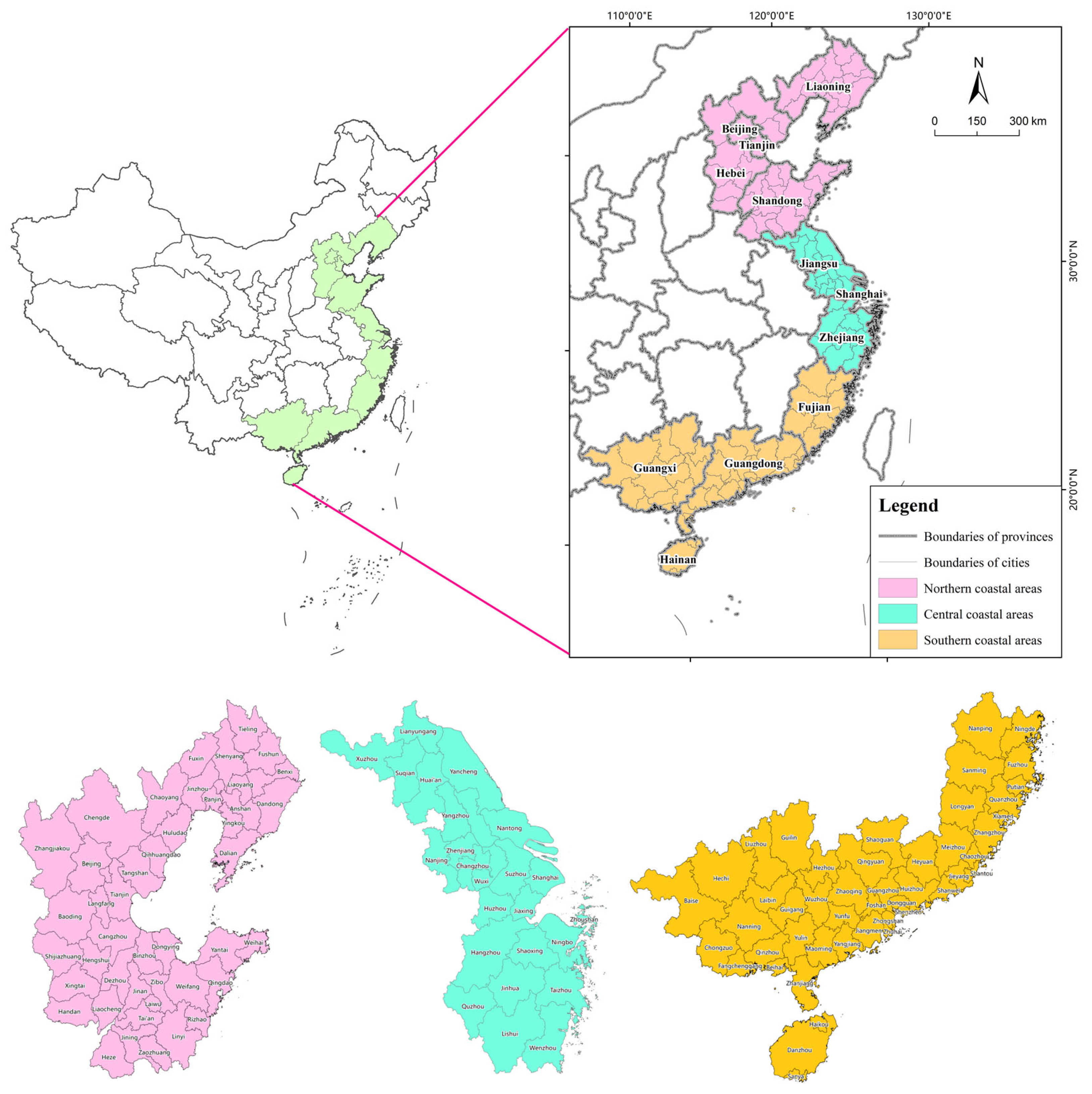
2.1. Study Area

The study area is defined as all the cities in China's coastal area, including Beijing, Shanghai, and Tianjin municipalities, and the coastal cities in Liaoning, Hebei, Shandong, Jiangsu, Zhejiang, Fujian, Guangdong, Guangxi, and Hainan provinces (Figure 1). The area is divided into three urban agglomerations, namely northern coastal areas, central coastal areas, and southern coastal areas from north to south. To facilitate the illustration and discussion of the results, prefecture-level cities are marked and illustrated in the figure. Among these cities, Sansha City is located in the southernmost part of Hainan Province, and its land area only accounts for less than 1% of the total area of the city, which makes it difficult to estimate the economic development status in large-scale studies. In addition, due to the lack of economic statistical data in some years since the establishment of Sansha City, it has not been included in the scope of research.

2.2. Data

The data used in this study include VIIRS data, LandScan data, land use data, and socioeconomic statistical data.

2.2.1. Visible Infrared Imaging Radiometer Suite (VIIRS) Nighttime Light Data

In this study, the nighttime light data for the years 2012, 2015, 2018, and 2021 were VIIRS data obtained from the National Oceanic and Atmospheric Administration (NOAA) National Center for Environmental Information. The VIIRS cloud-free composite data were generated monthly in the diurnal band with a spatial resolution of 15 arcseconds. Compared with Defense Meteorological Satellite Program (DMSP) data, VIIRS data have higher spatiotemporal resolution and better light resolution. At the same time, there was no supersaturation problem, and there was no need for inter-annual calibration and sensor calibration.

2.2.2. Landscan Data

The LandScan population dataset for 2012, 2015, 2018, and 2021 assisting nighttime light data in GDP spatialization was provided by the Oak Ridge National Laboratory. Compared with WorldPop, GHS-POP, GPW, and other gridded population datasets, LandScan has the best performance in terms of spatial accuracy and estimation error [23]. The gridded population is produced by interpolating subnational census population data to a 1 km × 1 km spatial resolution.

2.2.3. Land Use Data

National land use data were derived from the cloud platform of geographic national conditions monitoring. Landsat TM/ETM/OLI remote sensing images are the main data source for national land use data products. After image fusion, geometric correction, image enhancement, and splice, the land use types of the country are divided into 6 first-level categories through the method of human–computer interactive visual interpretation, 25 secondary, and some tertiary categories of land use data products. The average classification accuracy of the data in residential land, cultivated land, and industrial and mining land is above 85%. The study adopted 1km resolution land use data in 2012, 2015, 2018, and 2021, respectively.

2.2.4. Statistical Data

Regarding the prefecture-level statistical data, the social and economic statistical data such as annual GDP sub-industry data and population data came mainly from the China Urban Statistical Yearbook 2012, 2015, 2018, and 2021 [24] to facilitate the GDP spatial modeling and its accuracy improvement.

2.3. Data Pre-Processing

In order to ensure data accuracy, both raster and vector data in the aforementioned data were extracted and projected to an Albers equal-area conic projection with a spatial resolution of 1 km. Bilinear interpolation was used for continuous data such as luminous remote sensing data. The nearest neighbor resampling method was used for categorical data, such as land use data.

VIIRS luminous remote sensing data are divided into monthly composite data and annual composite data. The annual data eliminate noise and also eliminate the influence of auroral, fishing fire, cloud cover and sensor itself, etc. However, there are only two periods in 2015 and 2016, so it is difficult to obtain annual luminous remote sensing data with long-term stable series using the VIIRS annual data mask. Due to the irregular noise distribution of monthly data, there will be large noise differences in different regions between images during the same period, so it is necessary to de-noise the data to carry out further research.

Considering the impact of time difference on the accuracy of the mask, it is difficult to reflect the change in the city in the data. In this paper, a method of quarterly self-masking based on monthly composite data is proposed. The monthly data of each month were binarized into luminous and non-luminous areas using a raster calculator, and then the mask data for the twelve months were divided into four groups according to the quarter. The four quarters of data obtained by multiplying the data within the group are added and then binarized again using the raster calculator tool. The mask made by this method can remove unstable pixels, and the mask region will not be distorted due to the cloud cover of a certain month.

The self-mask can solve the problem of irregular distribution of low noise points. Taking Zhejiang Province and Shanghai Municipality in 2015 as an example, the masks made by means of monthly data, self-masking method, and annual composite data are shown in Figure 2. The results show that self-masking removes much noise and preserves the spatial structure left by the traffic network, and the self-masking method can also restore the true annual distribution of luminous. The correlation coefficient between the self-mask and the mask made by VIIRS annual data in spatial distribution is more than 0.9. The VIIRS annual data mask method has a time lag and cannot be used for the study of long time series. The timeliness and high reduction in the self-masking method were proved in this experiment, so the self-masking method was used instead of the VIIRS masking method.

2.4. Methods

The methodology of this study has the following four main aspects: (1) modeling GDP spatialization; (2) GDP spatial data multitemporal and multilevel change analyses; (3) GDP spatial pattern using local Moran; (4) standard deviation ellipse and economic center of the GDP spatial data development of China’s coastal areas.

2.4.1. Modeling GDP Spatialization

China’s total population, GDP, and other social and economic data are generally based on grass-roots administrative regions as the basic unit, through the census, sampling statistics, etc., after a step-by-step summary of the final form of two-dimensional tables. These data usually use relational databases for storage, retrieval, updating, data analysis, and information reproduction [25]. Grid socioeconomic data can not only reflect reality more intuitively and more closely but also provide a unified spatial benchmark for the integration of natural, economic, and social data and provide basic technical support for analyzing, simulating, and predicting the development and evolution of various socioeconomic factors [10,15]. The process of the GDP spatialization method was as follows. Firstly, the spatial GDP of each sector was calculated, and GDP₁, GDP_2, and GDP₃ were used to represent the primary industry, the secondary industry, and the tertiary industry, respectively. Then, the GDP results of each industry were added to obtain the overall GDP spatialization results. According to China’s National Economic Industry Classification and Three Industry Division Regulations, China’s GDP is divided into three industries for statistics, namely, the first industry (agriculture, forestry, animal husbandry, fishery), the second industry (mining, manufacturing, and other industries), and the tertiary industry (other industries outside the first/second industry, that is, the service industry). Since the primary industry was often closely related to natural resources, land use data and rural population spatial grid data were used to perform geographically weighted regression (GWR) on the GDP₁. Because the product of the second industry and the tertiary industry reflected human economic activities, nighttime light data were used for the calculation of GDP₂ and GDP₃.

Studies have shown that there was a significant correlation between primary industry, agricultural land, and rural population [26,27]. The study area is located in the coastal areas, and there is no large-scale animal husbandry, so the impact of the grassland area on the performance of the primary industry is not considered. The traditional research used the cultivated land area as the regression factor. In this study, the cultivated land was divided into paddy field area and dry land area. In addition, considering that the study areas are all coastal areas, the water area is further subdivided. After that, paddy field, dry land, forest land, river canal, lake, and pond reservoirs were selected as the explanatory variables of land use in the regression model, and rural population was selected as the explanatory variable of production.

The regression model of the primary industry GDP is as follows:

$$GD{P}_{1i}={\sum }_{j=1}^6{\alpha }_{ij}{S}_{ij }+\beta P_i+\gamma$$

(1)

where GDP_1i is the primary industry GDP value of the city_i, S_ij is the j land type in i city, P_i is the number of rural populations in the i city, α_ij and β are the proportion factors of j-type land area and rural population in the i city, and γ is a constant term.

The geographically weighted regression (GWR) model is constructed in the ArcGIS operating platform. The condition number field (COND) in the GWR output indicates when results are unstable due to local multicollinearity. Results associated with condition numbers larger than 30 are not reliable. Explanatory variables include the land use data and spatial data of rural populations. The Gaussian adaptive kernel function is selected for the kernel type. The parameters of various land types in each prefecture-level city obtained by regression are transformed into vector grids, and then the parameter grids are multiplied by the land use type grids to obtain the primary industry output value per square kilometer of each land type in each prefecture-level city. According to the division of the output value of the primary industry and the real output value of each prefecture-level city obtained by statistics, the correction coefficient is calculated to correct the numerical deviation generated in the fitting process, and the unbiased spatialized km grid data of the output value of the primary industry at the prefecture-level city level in 2012, 2015, 2018, and 2021 are obtained.

Many studies have shown that the luminous intensity of remote sensing images is closely related to the range and GDP value of the secondary/tertiary industries [11,28]. The second and tertiary industries are mainly concentrated in the built-up areas of the city, and the intensity and scope of luminous reflect the intensity and scope of economic activities.

Total light intensity (TNL), average relative light intensity (ALI), light area ratio (LAR), and comprehensive light index (CNLI) were constructed [29], and the calculation formula was as follows:

$$TNL={\sum }_{i=1}^{n}D{N}_i$$

(2)

$$ALI={\sum }_{i=1}^n\left(\frac{D{N}_i}{D{N}_{max}}\right)$$

(3)

$$LAR=\frac{A_l}{A}$$

(4)

$$CNLI=\mathrm{ALI}\times \mathrm{LAR}$$

(5)

where DN_i represents the luminous intensity value in the administrative unit; n represents the total number of pixels in the administrative unit; and A_l and A represent the luminous area (DN > 0) and the total area of the administrative unit, respectively.

The GWR model was constructed based on the ArcGIS software platform. GDP was taken as the dependent variable, TNL, ALI, LAR, CNLI, and urban population as explanatory variables, the Gaussian adaptive kernel function was selected as the kernel type, and AICc was selected to determine the bandwidth of the kernel function.

The results after GWR were distributed on the grid, and the distribution formula is as follows:

$$GD{P}_{23i}=GD{P}_{23predict}\times \left(\frac{D{N}_i}{NTL}\right)$$

(6)

where GDP₂₃ predict is the predicted output value of the second and third industries of each prefecture-level city obtained by GWR regression; GDP_23i is the output value of the second/third industry of the i pixel, that is, the economic density of the output value; DN_i is the brightness value of the i-th pixel; and NTL is the total pixel value of prefecture-level cities.

2.4.2. Local Moran’s I-Statistic

Moran’s index was used to analyze the spatial distribution of GDP. The global Moran index was used to analyze whether there is a spatial correlation, and the local Moran index was used to reflect the spatial correlation of regional GDP. The computational formula of the local Moran’s I index was as follows:

$$I_i=\frac{Z_i}{S^2}{\sum }_{j\ne i}^n{\omega }_{i,j}{Z}_j$$

(7)

where n is the total number of regions studied, ω_i,j is the spatial weight value, I_i is the local Moran index of region I, Z_j and Z_i are the degree of deviation from the mean of the factor attributes of region j and region i, respectively, and S is the square average of the deviation of each region.

There are two types of positive spatial association, namely, spatial units with attribute values higher than the mean are surrounded by neighborhoods with attribute values higher than the mean (high-high association, HH), and spatial units with attribute values lower than the mean are surrounded by neighborhoods with attribute values lower than the mean (low-low association, LL). There are also two types of negative spatial association, namely, spatial units with attribute values higher than the mean are surrounded by neighborhoods with attribute values lower than the mean (high-low association, HL) or the opposite (low-high association, LH) [30].

2.4.3. Standard Deviational Ellipse (SDE) Model

The SDE model is widely used in the study of economic patterns and urban evolution and development [27]. The size of the ellipse reflects the concentration degree of the overall elements of the spatial pattern, and the declivity angle (long axis) reflects the dominant direction of the pattern [31]. The position of the center of gravity represents the geographical center of the economic data distribution in the study area, and the coordinate migration of this point reflects the trend of economic development of urban agglomerations. Hence, this method is selected in this study to investigate the spatial evolution of economic development, which is performed using ArcGIS (version 10.2).

The calculation formula is as follows:

$$G_x=\frac{{\sum }_{i=1}^n{w}_i{x}_i}{{\sum }_{i=1}^n{w}_i}, G_y=\frac{{\sum }_{i=1}^n{w}_i{y}_i}{{\sum }_{i=1}^n{w}_i}$$

(8)

$$\mathit{tan}\theta =\frac{\left({\sum }_{i=1}^n{\tilde{x}}_i^2-{\sum }_{i=1}^n{\tilde{y}}_i^2\right)+\sqrt{{\left({\sum }_{i=1}^n{\tilde{x}}_i^2-{\sum }_{i=1}^n{\tilde{y}}_i^2\right)}^2+4{\left({\sum }_{i=1}^n,{\tilde{x}}_i,{\tilde{y}}_i\right)}^2}}{2{\sum }_{i=1}^n{\tilde{x}}_i{\tilde{y}}_i}$$

(9)

$${\sigma }_x=\sqrt{2}\sqrt{\frac{{\sum }_{i=1}^n({\tilde{x}}_i\cos \theta -{\tilde{y}}_i\sin \theta {)}^2}{n}}, {\sigma }_y=\sqrt{2}\sqrt{\frac{{\sum }_{i=1}^n({\tilde{y}}_i\cos \theta +{\tilde{x}}_i\sin \theta {)}^2}{n}}$$

(10)

where G_x and G_y represent the x-axis coordinate and y-axis coordinate of the ellipse center; w_i represents the indicator weight; x_i and y_i are the deviations of the average center from the x-axis and y-axis coordinates; θ represents the azimuthal angle of the ellipse; and σ_x and σ_y are the major and minor axis lengths of the ellipse, respectively.

3. Results and Discussion

3.1. GDP Spatialization

In this study, land use data and rural population spatial grid data were used to perform GWR on the GDP₁. NTL indices were constructed from VIIRS data of China’s coastal provinces, and the results were subjected to a GWR model on GDP₂/GDP₃. The model parameters of the GDP spatialization model are provided in

Table 1. Evaluation index of GDP spatialization model.

Time	GDP1			GDP2/GDP3
	${\mathit{R}}^2$	Residual Sum of Squares	COND	${\mathit{R}}^2$	Residual Sum of Squares	COND
2012	0.74	3.18 × 1013	7.61	0.94	8.07 × 1015	15.89
2015	0.79	4.45 × 1013	7.50	0.92	1.69 × 1016	11.99
2018	0.77	5.41 × 1013	7.39	0.90	3.90 × 1016	12.83
2021	0.71	7.25 × 1013	7.54	0.85	9.05 × 1016	4.95

. The results show that correlation coefficient (R²) values were between 0.71 and 0.94. The condition number (COND) of GWR was less than 30, so there was no multicollinearity problem, indicating that the result was reliable.

Socioeconomic statistics are usually aggregated data at administrative levels, such as the town, which is the basic statistical unit in China [32]. Although statistics can reflect the differences among statistical units, they cannot reflect the heterogeneity within statistical units [15,33]. In practical application, it cannot meet the needs of socioeconomic data in any statistical region, and the spatialization of socioeconomic statistical data with NTL data is an important way to effectively solve this problem [34]. GDP density distribution maps for 2012, 2015, 2018, and 2021 were generated by VIIRS data and showed the GDP density within each 1 km pixel (Figure 3). We obtained an overview of the development of coastal areas. There were no significant changes in the spatial distribution of higher-GDP areas from 2012 to 2021. From north to south, the GDP density was concentrated in the Beijing–Tianjin–Hebei urban agglomeration, the Yangtze River Delta, and the Pearl River Delta, respectively. The three urban agglomerations have become the most urbanized and economically developed regions of China since the reform and opening up in 1978 [35]. However, in 2021, the red high-value area decreased significantly in Liaoyang of Liaoning Province, Shaoguan of Guangdong Province, and Quzhou of Zhejiang Province compared with 2012 (Figure 3a). Meanwhile, by 2021, several patches of red high-value area can be found on the side close to the sea, both in central and southern coastal areas (Figure 3b,c).

3.2. GDP Spatial Autocorrelation

Analyzing the spatial autocorrelation of the economic data could have better performance than pixel-level data on GDP spatialization. The local spatial autocorrelation analysis can reveal the degree of agglomeration and dispersion of a region and adjacent regions within a local area [36]. The GDP spatial autocorrelation of three coastal areas in 2012, 2015, 2018, and 2021 were assessed by local Moran index analysis. Overall, as shown in Figure 4, a relatively stable space distribution of HH cluster areas occurred mostly in the Beijing–Tianjin–Hebei urban agglomeration, the Yangtze River Delta, and the Pearl River Delta from 2012 to 2021, indicating that the three agglomerations show a high level of spatial agglomeration effect of economic development with neighboring areas. It is worth noting that the HH cluster region of the Yangtze River Delta in the central coastal area is the largest since 2012, indicating that the agglomeration has a relatively high urbanization rate.

In the northern coastal areas, Liaoning Province exhibited the most severe area growth in the LL cluster by 2021, while the HH cluster area around Shenyang and Dalian was significantly reduced (Figure 4a), meaning that the economic growth of the region was low during this period. Gao and Chen [37] also found a downward trend of economic growth from the Shenyang and Dalian Economic Belt toward both sides from 2009 to 2019. In general, in the northeast of China, such as Liaoning Province, the level of urban economic development is relatively low, and the transformation pressure of resource-based cities is greater [38]. Though Liaoning Province is one of the main parts of the old industrial base, the economic stagnation in Liaoning and other northeast areas of China showed a sharp contrast with the rapid economic growth from 2012 to 2021 [39]. Due to the obvious restriction of industrial efficiency and benefit shortboard, the advantages of heavy industry have greatly shifted [40,41]. The spatial agglomeration feature and regional competitiveness have weakened [37,42]. In the Beijing–Tianjin–Hebei region, Beijing was developed as the central city under the guidance of the policies. During the study period, the LL cluster areas of Hebei Province also show a certain expansion trend in Hebei Province. Moreover, the HH cluster area of the Tianjin area also declined obviously (Figure 4a). This may be due to Beijing’s implementation of a series of administrative policies to encourage the reduction of the secondary industry and the development of the tertiary industry before the secondary industry was fully developed and transferred to neighboring cities, resulting in a delay in the integration process and development of the Beijing–Tianjin–Hebei agglomeration [43,44].

In the central coastal areas, the LL cluster areas located in Quzhou, Lishui, and Wenzhou of south Zhejiang Province from 2012 to 2021 decreased gradually (Figure 4b), indicating an improving trend of economic growth. The concept of “ecological civilization” as the context of Chinese policy first appeared in the report of the 17th National Congress of the Communist Party of China (CPC), published in October 2007 [45]. In 2012, the 18th National Congress of the CPC elevated ecological civilization construction to a particularly prominent position, integrating it with economic, political, cultural, and social construction [46]. The development of green finance became a vital method to achieve coordinate economic and environmental development. With the support of national policies, the green finance development of Zhejiang is better than that of other provinces in the same region [47]. As one of the national innovation pilot zones in green finance, Zhejiang focuses on innovating green finance services for the transformation and upgrading of traditional industries [48]. The development of green finance, as the grip for economic transformation, provides financial support for regional scientific and technological innovation and the upgrading of energy consumption structure, thereby promoting the flow of capital to green low-energy industries and thus achieving economic development [49]. In the southern coastal areas, the HH clusters of GDP density are mainly concentrated in the central coastal area of Guangdong, and a new HH cluster occurred in Quanzhou of Fujian Province, as shown in Figure 4c, indicating an upward trend of economic growth along the coast from 2012 to 2021. Simultaneously, a shrinking trend of the LL cluster areas was observed in Guangxi, Guangdong, Fujian, and Hainan from 2012 to 2021 (Figure 4c). The Pearl River Delta is a hinge region for the southern regions of China to enter into the One Belt and One Road [50]. In 2015, the Chinese government further released the “Promoting the Construction of the Silk Road Economic Belt and the 21st Century Vision and Actions for the Maritime Silk Road” and emphasized the construction of 15 node seaports [51]. As node seaports, Quanzhou in Fujian Province, Guangzhou and Shenzhen in Guangdong Province, and Haikou and Sanya in Hainan Province play a critical role in promoting the “Belt and Road”. Among them, Guangzhou and Shenzhen, as two node ports with the highest economic level and competitiveness next to Shanghai in China, have played a great role in promoting regional economic development and deepening global integration [52]. Although Haikou and Sanya, two node port cities in Hainan Province, have strong development potential, their economic level and competitiveness are relatively weak. Although Haikou and Sanya, two node port cities in Hainan Province, have strong development potential, they rank the lowest in terms of port infrastructure and economic level [53]. Therefore, it has not completely changed the characteristics of economic agglomeration in Hainan Province, as shown in Figure 4c.

3.3. Spatiotemporal Changes in GDP Density

To clearly show the process of the economic pattern of typical regions, the Liaoning sample area, the Shanghai–Suzhou–Hangzhou sample area, and the Pearl River Delta sample area were selected for further analysis. The GDP density changes within each 1km pixel of the three sample areas were generated. As Figure 5a shows, the year 2018 is an important node for economic development in the three sample areas. From 2018 to 2021, the economic growth rate of the Liaoning sample area improved greatly compared with previous years. Consistent with the results of this study, Li [54] also found that Shenyang’s economy declined from 2014 to 2018 and rebounded in 2018 through three dimensions of evaluation of economy, society, and environment. The downturn before 2018 is the result of combined influences, including inadequate policy implementation [55] and the deficiency of industrial structure transformation [56]. After 2018, with the in-depth implementation of policies, such as the “Shenyang Economic Belt” and “Liaoning Coastal Economic Belt”, Shenyang radiates to the surrounding cities and promotes development [57]. The economic growth of the other two sample areas, the two most developed urban agglomerations, showed a trend of first growth and then decline, with 2018 as the turning point (Figure 4b,c). This may be due to the outbreak of the COVID-19 pandemic in 2019, which made the world face an unprecedented global health, social, and economic incident. Recent research shows that the pandemic seriously disrupted global value chains and limited economic growth [58]. China's eastern coastal region, especially Shanghai, is the most directly affected city. The lockdown in Shanghai undoubtedly had a negative impact and weakened the intensity of human and economic activities in neighboring cities due to the close relationship between Shanghai and the Yangtze Revier Delta [59].

3.4. Spatiotemporal Patterns and Evolution in Coastal Economy

The SDE model is one of the classical methods to analyze the directivity of spatial distribution. Using a standard deviation ellipse, we can quantitatively explain the centrality, directionality, and dispersion of the spatial and temporal distribution of socioeconomic indicators [60]. The SDE model results are shown in

Table 2. The SDE model parameters of economic development in the study area from 2012 to 2021.

Area	Year	Center Longitude (°E)	Center Latitude (°N)	X-Axis (km)	Y-Axis (km)	Azimuth (°)
The whole study area	2012	118.0856	32.1942	730,141.43	2,132,049.28	0.17
	2015	117.8906	31.7282	738,943.03	2,129,774.58	1.00
	2018	117.8382	31.3219	735,111.07	2,067,388.21	0.93
	2021	118.3380	31.6988	740,359.19	2,048,891.41	0.83
Northern coastal areas	2012	118.7561	38.9095	502,319.79	703,394.83	25.54
	2015	118.5788	38.8530	517,234.72	656,415.68	21.84
	2018	118.2986	38.6236	515,950.05	618,080.16	5.31
	2021	118.2667	38.5792	516,480.23	664,877.02	9.07
Central coastal areas	2012	120.4783	31.2813	203,279.27	438,901.17	142.32
	2015	120.4367	31.3141	198,933.07	439,933.22	141.20
	2018	120.4034	31.3361	194,785.30	447,548.90	141.89
	2021	120.3552	31.2943	201,499.53	480,798.15	144.86
Southern coastal areas	2012	114.1477	23.2679	738,255.73	256,922.02	55.85
	2015	114.0654	23.2240	725,658.92	257,944.38	56.11
	2018	114.2501	23.2739	734,458.80	247,961.40	54.35
	2021	114.4843	23.4011	793,775.73	253,102.07	53.05

and

Table 3. Elliptic moving parameters of the SDE model of economic development in the study area.

Area	Center of Gravity
	Distance(km)	Direction
The whole study areas	59.96	South
Northern coastal areas	57.08	Southwest
Central coastal areas	11.84	Northwest
Southern coastal areas	37.45	Northeast

. From 2012 to 2021, the evolution trajectory of the economic center of gravity of the coastal economic belt generally moved southward, slightly skewed in the east–west direction. The moving distance of the economic center of gravity of the three coastal regions is northern coastal areas, southern coastal areas, and central coastal areas in order from high to low (Table 3). The change in China’s economic gravity center is closely related to the change in its population gravity center [61]. Previous studies have shown that China’s demographic center of gravity has also shifted southward since the reform and opening up [62]. The result of our study is consistent with the research results of Liang et al. [63], mainly due to the rapid rise in China’s Internet, AI, and other high-tech industries since 2013 and the significant trend of innovation driving in the Pearl River Delta and Yangtze River Delta [64].

The SDE results also showed that there were significant differences in the direction of the economic center of gravity evolution of the three coastal economic zones from 2012 to 2021 (Table 3). Figure 6 shows the process of the economic gravity center migration direction of the three coastal areas during the study period. The economic gravity center in the northern coast areas moved to the southwest, and the distance of the center of gravity was 57.08 km. According to the change in geographic coordinates of the center of gravity, it can be seen that the southward movement speed and distance are the highest from 2015 to 2018 (Table 2 and Figure 6a), which was probably caused by the economic decline and shrinking population and the weakening of the regional economic driving ability of Liaoning Province during this period [63] The economic gravity center in the central region is the most stable, and the total moving distance was 11.84 km. As shown in Figure 4b, with 2018 as a turning point, the economic center of gravity shifted from northwest to southwest, moving toward the mainland. This result confirms the greater economic impact of the pandemic on Shanghai. It also suggested that the gap between the surrounding areas and Shanghai, the economic center of the Yangtze River Delta, is narrowing. This could be due to the digital economy significantly promoting the rationalization and advancement of industrial structure in the Yangtze River Delta [65]. In the southern coastal areas, the economic center of gravity always fell in Huizhou of Guangdong Province, while the moving direction shifted significantly, with 2015 as a turning point (Figure 6c). The results show that Guangxi has been at a relatively backward level during the study period, which is consistent with the characteristics of economic agglomeration mentioned above (Figure 4). Compared with other coastal provinces, Guangxi’s existing economic foundation is weak, and Guangxi has not received policy support for node seaports construction. On the contrary, Fujian Province has formed Quanzhou, the new economic agglomeration area, through coastal economic construction, which has promoted the moving of the economic gravity center to a certain extent. In addition, due to the huge gap between Hainan Province and Guangdong Province in port city construction and economic level, regional economic development is relatively slow [53], resulting in a gradual departure from the economic center of gravity.

4. Conclusions

In this study, the economic development pattern of China's coastal areas from 2012 to 2021 was spatialized at the 1km grid scale based on the combination of NPP/VIIRS NTL data and statistical data. The spatial characteristics of GDP and its changes within three coastal agglomerations were analyzed in detail. The developed grided GDP map shows a better performance in presenting the distribution and activities of economic development. The results demonstrated that the Yangtze River Delta was extremely active, and the economic development of the northern coastal areas needs to be strengthened. Additionally, the grided GDP data can serve as an important supplement to small-scale socioeconomic development data and provide guidance for regional strategy and policy decision making. The method proposed in this study also provides an opportunity for researchers to explore the evolution process and mechanism of economic development in the Belt and Road region.

References

1. Liu, W. Scientific understanding of the Belt and Road Initiative of China and related research themes. Prog. Geogr. 2015, 34, 538–544. [Google Scholar]
2. Liu, W.; Hughes, A.C.; Sachdeva, G.; Narain, D.; Zhou, T.D.; Wang, Y.; Gallagher, K.; Turschwell, M.; Tian, X.; Han, M.Y. The Belt and Road Initiative and the Sustainable Development Goals. One Earth 2020, 3, 263–267. [Google Scholar] [CrossRef]
3. Huang, Y. Understanding China’s Belt & Road Initiative: Motivation, framework and assessment. China Econ. Rev. 2016, 40, 314–321. [Google Scholar]
4. China National Development and Reform Commission. 2015. Available online: https://www.gov.cn/xinwen/2015-03/28/content_2839723.htm (accessed on 21 January 2024).
5. Elvidge, C.D.; Baugh, K.E.; Kihn, E.A.; Kroehl, H.W.; Davis, E.R.; Davis, C.W. Relation between satellite observed visible-near infrared emissions, population, economic activity and electric power consumption. Int. J. Remote Sens. 1997, 18, 1373–1379. [Google Scholar] [CrossRef]
6. Shi, K.; Yu, B.; Zhou, Y.; Chen, Y.; Yang, C.; Chen, Z.; Wu, J. Spatiotemporal variations of CO2 emissions and their impact factors in China: A comparative analysis between the provincial and prefectural levels. Appl. Energy 2019, 233–234, 170–181. [Google Scholar] [CrossRef]
7. Bustos, M.F.A.; Hall, O.; Andersson, M. Nighttime lights and population changes in Europe 1992–2012. Ambio 2015, 44, 653–665. [Google Scholar] [CrossRef] [PubMed]
8. Zhou, Y.Y.; Smith, S.J.; Elvidge, C.D.; Zhao, K.G.; Thomson, A.; Imhoff, M. A cluster-based method to map urban area from DMSP/OLS nightlights. Remote Sens. Environ. 2014, 147, 173–185. [Google Scholar] [CrossRef]
9. Small, C.; Pozzi, F.; Elvidge, C.D. Spatial analysis of global urban extent from DMSP-OLS night lights. Remote Sens. Environ. 2005, 96, 277–291. [Google Scholar] [CrossRef]
10. Bennett, M.M.; Smith, L.C. Advances in using multitemporal night-time lights satellite imagery to detect, estimate, and monitor socioeconomic dynamics. Remote Sens. Environ. 2017, 192, 176–197. [Google Scholar] [CrossRef]
11. Chen, Z.Q.; Yu, B.L.; Yang, C.S.; Zhou, Y.Y.; Yao, S.J.; Qian, X.J.; Wang, C.X.; Wu, B.; Wu, J.P. An extended time series (2000–2018) of global NPP-VIIRS-like nighttime light data from a cross-sensor calibration. Earth Syst. Sci. Data 2021, 13, 889–906. [Google Scholar] [CrossRef]
12. Zhao, M.; Zhou, Y.Y.; Li, X.C.; Zhou, C.H.; Cheng, W.M.; Li, M.C.; Huang, K. Building a Series of Consistent Night-Time Light Data (1992–2018) in Southeast Asia by Integrating DMSP-OLS and NPP-VIIRS. IEEE Trans. Geosci. Remote Sens. 2020, 58, 1843–1856. [Google Scholar] [CrossRef]
13. Li, P.; Zhang, H.R.; Wang, X.; Song, X.; Shibasaki, R. A spatial finer electric load estimation method based on night-light satellite image. Energy 2020, 209, 118475. [Google Scholar] [CrossRef]
14. Zhou, Y.; Chen, M.; Tang, Z.; Zhao, Y. City-level carbon emissions accounting and differentiation integrated nighttime light and city attributes. Resour. Conserv. Recycl. 2022, 182, 106337. [Google Scholar] [CrossRef]
15. Chen, X.; Nordhaus, W.D. Using luminosity data as a proxy for economic statistics. Proc. Natl. Acad. Sci. USA 2011, 108, 8589–8594. [Google Scholar] [CrossRef] [PubMed]
16. Chen, X.; Nordhaus, W.D. VIIRS nighttime lights in the estimation of cross-sectional and time-series GDP. Remote Sens. 2019, 11, 1057. [Google Scholar] [CrossRef]
17. Doll, C.N.H.; Muller, J.P.; Elvidge, C.D. Night-time imagery as a tool for global mapping of socioeconomic parameters and greenhouse gas emissions. AMBIO J. Hum. Environ. 2000, 29, 157–162. [Google Scholar] [CrossRef]
18. Keola, S.; Andersson, M.; Hall, O. Monitoring economic development from space: Using nighttime light and land cover data to measure economic growth. World Dev. 2015, 66, 322–334. [Google Scholar] [CrossRef]
19. Sutton, P.C.; Costanza, R. Global estimates of market and nonmarket values derived from nighttime satellite imagery, land cover, and ecosystem service valuation. Ecol. Econ. 2002, 41, 509–527. [Google Scholar] [CrossRef]
20. Li, X.; Xu, H.; Chen, X.; Li, C. Potential of NPP-VIIRS nighttime light imagery for modeling the regional economy of China. Remote Sens. 2013, 5, 3057–3081. [Google Scholar] [CrossRef]
21. Chen, Q.; Hou, X.Y.; Zhang, X.C.; Ma, C. Improved GDP spatialization approach by combining land-use data and night-time light data: A case study in China’s continental coastal area. Int. J. Remote Sens. 2016, 37, 4501–4730. [Google Scholar] [CrossRef]
22. Wu, J.; Wang, Z.; Li, W.; Peng, J. Exploring Factors Affecting the Relationship between Light Consumption and GDP Based on DMSP/OLS Nighttime Satellite Imagery. Remote Sens. Environ. 2013, 134, 111–119. [Google Scholar] [CrossRef]
23. Yin, X.; Li, P.; Feng, Z.M.; Yang, Y.Z.; You, Z.; Xiao, C.W. Which Gridded Population Data Product Is Better? Evidences from Mainland Southeast Asia (MSEA). ISPRS Int. J. Geo-Inf. 2021, 10, 681. [Google Scholar] [CrossRef]
24. National Bureau of Statistics of China. Available online: https://www.stats.gov.cn/sj/ndsj/ (accessed on 21 January 2024).
25. Hu, Y.; Wang, Q.; Liu, Y.; Li, J.; Ren, W. Index System and Transferring Methods to Build the National Society and Economy Grid Database. J. Geo-Inf. Sci. 2011, 13, 573–578. [Google Scholar] [CrossRef]
26. Wang, S.T.; Bai, X.M.; Zhang, X.L.; Reis, S.; Chen, D.L.; Xu, J.M.; Gu, B.J. Urbanization can benefit agricultural production with large-scale farming in China. Nat. Food 2021, 2, 183–191. [Google Scholar] [CrossRef] [PubMed]
27. Lanz, B.; Dietz, S.; Swanson, T. Global Economic Growth and Agricultural Land Conversion under Uncertain Productivity Improvements in Agriculture. Am. J. Agric. Econ. 2018, 100, 545–569. [Google Scholar] [CrossRef]
28. Mccord, G.C.; Roriguez-Heredia, M. Nightlights and Subnational Economic Activity: Estimating Departmental GDP in Paraguay. Remote Sens. 2022, 14, 115. [Google Scholar] [CrossRef]
29. Zhao, M.; Cheng, W.M.; Zhou, C.H.; Li, M.C.; Wang, N.; Liu, Q.Y. GDP spatialization and economic differences in South China based on NPP-VIIRS nighttime light imagery. Remote Sens. 2017, 9, 673. [Google Scholar] [CrossRef]
30. Anselin, L. Local indicators of spatial association-LISA. Geogr. Anal. 1995, 27, 93–115. [Google Scholar] [CrossRef]
31. Gong, J. Clarifying the standard deviational ellipse. Geogr. Anal. 2002, 34, 155–167. [Google Scholar] [CrossRef]
32. Liang, H.D.; Guo, Z.Y.; Wu, J.P.; Chen, Z.Q. GDP spatialization in Ningbo City based on NPP/VIIRS night-time light and auxiliary data using random forest regression. Adv. Space Res. 2019, 65, 481–493. [Google Scholar] [CrossRef]
33. Guo, H.X.; Zhu, W.Q. A review on the spatial disaggregation of socioeconomic statistical data. Acta Geogr. Sin. 2022, 77, 2650–2667. [Google Scholar]
34. Zhao, Z.Z.; Tang, X.J.; Wang, C.; Cheng, G.; Ma, C.; Wang, H.T.; Sun, B.K. Analysis of the Spatial and Temporal Evolution of the GDP in Henan Province Based on Nighttime Light Data. Remote Sens. 2023, 15, 716. [Google Scholar] [CrossRef]
35. Li, W.W.; Yi, P.T.; Yu, H.T.; Lin, W.C.; Wu, X.Y. Assessment on sustainable development of three major urban agglomerations in China based on sustainability-differentiation-combined weighting method. Sustain. Dev. 2023, 31, 2678–2693. [Google Scholar] [CrossRef]
36. Koo, H.; Chun, Y.W.; Wong, D.W. Measuring Local Spatial Autocorrelation with Data Reliability Information. Prof. Geogr. 2021, 73, 464–480. [Google Scholar] [CrossRef]
37. Gao, Y.; Chen, W. Study on the coupling relationship between urban resilience and urbanization quality-A case study of 14 cities of Liaoning Province in China. PLoS ONE 2021, 16, e0244024. [Google Scholar] [CrossRef]
38. Liang, Y.Y.; Yi, P.T.; Li, W.W.; Liu, J.; Dong, Q.K. Evaluation of urban sustainability based on GO-SRA: Case study of Ha-Chang and Mid-southern Liaoning urban agglomerations in northeastern China. Sustain. Cities Soc. 2022, 87, 104234. [Google Scholar] [CrossRef]
39. Gao, H.; Taniguchi, Y. Revitalization of the Economy of Northeast China. In Industrial Location and Vitalization of Regional Economy; Ishikawa, T., Nakamura, D., Eds.; Springer: Singapore, 2023. [Google Scholar]
40. Tian, S.C.; Zhang, W.Z. Evolution of spatial pattern of Chinese iron and steel industry and the influencing factors. Prog. Geogr. 2009, 28, 537–545. [Google Scholar]
41. Mao, X.Y.; Liu, Y.; He, C.F. Spatial pattern dynamics of resource-based industry in China. J. Nat. Resour. 2015, 30, 1332–1342. [Google Scholar]
42. Wang, S.J.; Ma, L. Strategic thinking of Northeast China revitalization during the “14th Five-Year Plan” based on the macro situation and regional advantages. Sci. Geogr. Sin. 2021, 41, 1935–1946. [Google Scholar]
43. Niu, F.Q.; Yang, X.Y.; Wang, F. Urban Agglomeration Formation and Its Spatiotemporal Expansion Process in China: From the Perspective of Industrial Evolution. Chin. Geogr. Sci. 2020, 30, 532–543. [Google Scholar] [CrossRef]
44. Wang, Y.F. Population-land urbanization and comprehensive development evaluation of the Beijing-Tianjin-Hebei urban agglomeration. Environ. Sci. Pollut. Res. 2020, 29, 59862–59871. [Google Scholar] [CrossRef] [PubMed]
45. Xue, B.; Han, B.; Li, H.Q.; Gou, X.H.; Yang, H.; Heiko, T.; Stefan, S. Understanding ecological civilization in China: From political context to science. Ambio 2023, 52, 1895–1909. [Google Scholar] [CrossRef] [PubMed]
46. Hansen, M.H.; Li, H.T.; Svarverud, R. Ecological civilization: Interpreting the Chinese past, projecting the global future. Glob. Environ. Change 2018, 53, 195–203. [Google Scholar] [CrossRef]
47. Lv, C.C.; Bian, B.C.; Lee, C.C.; He, Z.W. Regional gap and the trend of green finance development in China. Energy Econ. 2021, 102, 105476. [Google Scholar] [CrossRef]
48. Huang, X.L.; Zhu, R.; Wu, X.X.; Ge, P.F. Assessing the role and driving mechanisms of the green financial reform on urban energy consumption and pollution emissions: A policy evaluation from the generalized synthetic control method. Environ. Sci. Pollut. Res. 2023, 30, 119095–119116. [Google Scholar] [CrossRef] [PubMed]
49. Yao, F.G.; Song, Y.; Xue, L.Q. Study on the effect of green financial policies on low-carbon economic development based on evidence from green financial reform and innovation pilot zone. Environ. Sci. Pollut. Res. 2023, 30, 74598–74611. [Google Scholar] [CrossRef] [PubMed]
50. Lu, D.D. Development of Pearl River Delta Metropolitan Group and Pan-Pearl River Delta Economic Cooperation Zone. Econ. Geogr. 2017, 37, 1–4. [Google Scholar]
51. Huo, W.W.; Zhang, W.; Peggy, S.L.C. Recent development of Chinese port cooperation strategies. Res. Transp. Bus. Manag. 2018, 26, 67–75. [Google Scholar] [CrossRef]
52. Chen, C.; Song, F.F. Evaluation of Port Logistics Competitiveness in China along the Belt and Road. J. Coast. Res. 2019, 93, 1117–1124. [Google Scholar] [CrossRef]
53. Wang, J.; Mo, L.L.; Ma, Z. Evaluation of port competitiveness along China’s “Belt and Road” based on the entropy-TOPSIS method. Sci. Rep. 2023, 13, 15717. [Google Scholar] [CrossRef]
54. Li, W.W.; Yi, P.T.; Zhang, D.N. Investigation of sustainability and key factors of Shenyang city in China using GRA and SRA methods. Sustain. Cities Soc. 2021, 68, 102796. [Google Scholar] [CrossRef]
55. Zhao, R.; Wang, Y. On the causes and countermeasures of the “Northeast Phenomenon". Nankai J. (Philos. Lit. Soc. Sci. Ed.) 2017, 6, 56–64. [Google Scholar]
56. Li, B.X.; Wang, H. Comprehensive evaluation of urban high-quality development: A case study of Liaoning Province. Environ. Dev. Sustain. 2023, 25, 1809–1831. [Google Scholar] [CrossRef]
57. Tian, S.Z.; Jiang, J.L.; Li, H.; Li, X.M.; Yang, J.; Fang, C.L. Flow space reveals the urban network structure and development mode of cities in Liaoning, China. Humanit. Soc. Sci. Commun. 2023, 10, 257. [Google Scholar] [CrossRef]
58. Guan, D.; Wang, D.; Hallegatte, S.; Davis, S.J.; Huo, J.; Li, S.P.; Bai, Y.C.; Lei, T.Y.; Xue, Q.Y.; Coffman, D.; et al. Global supply-chain effects of COVID-19 control measures. Nat. Hum. Behav. 2020, 4, 577–587. [Google Scholar] [CrossRef]
59. Jiang, L.; Liu, Y. China’s Largest City-Wide Lockdown: How Extensively Did Shanghai COVID-19 Affect Intensity of Human Activities in the Yangtze River Delta? Remote Sens. 2023, 15, 1989. [Google Scholar] [CrossRef]
60. Xu, Y.Y.; Liu, Y.; Chen, R.D.; Men, Y.F.; Li, K.N.; Fu, C. Study on the spatio-temporal evolution characteristics and driving mechanism of China’s carbon emissions. Humanit. Soc. Sci. Commun. 2023, 10, 786. [Google Scholar] [CrossRef]
61. Gong, S.S.; Xiao, K.M. A Quantitative Study on the Spatio-temporal Changes of China’s Economic Centers of Gravity for the Past 2000 Years: A Proxy Analysis Based on Population and City Data. Sci. Geogr. Sin. 2021, 41, 1587–1597. [Google Scholar]
62. Liang, L.W.; Chen, M.X.; Luo, X.Y.; Xian, Y. Changes pattern in the population and economic gravity centers since the Reform and Opening up in China: The widening gaps between the South and North. J. Clean. Prod. 2021, 310, 127379. [Google Scholar] [CrossRef]
63. Liang, L.W.; Xian, L.; Chen, M.X. Economic Geography. Evolution Trend and Influencing Factors of Regional Population and Economy Gravity Center in China Since the Reform and Opening-up. Econ. Geogr. 2022, 42, 93–103. [Google Scholar]
64. Li, S.T.; Huang, Y.; Liu, Y.Z. Characteristics and Enlightenment of China’s Industrial Gravity Center Movement. Econ. Geogr. 2022, 42, 1–10. [Google Scholar]
65. Chang, K.; Zhang, H.J.; Li, B.Y. The Impact of Digital Economy and Industrial Agglomeration on the Changes of Industrial Structure in the Yangtze River Delta. J. Knowl. Econ. 2023. [Google Scholar] [CrossRef]
Figure 1. The location of the study area.
Sustainability 16 01255 g001
Figure 2. Spatial distribution of mask denoising results in Zhejiang Province (where 0 is the non-luminous region, 1 is the luminous region; (a) monthly data mean raw luminous remote sensing image in 2015; (b) quarterly self-masking denoising results image; (c) 2015 annual composite VIIRS data mask).
Sustainability 16 01255 g002
Figure 3. GDP spatialization of coastal areas in China, 2012–2021. (a) indicates the northern coastal areas, (b) indicates the central coastal areas, and (c) indicates the southern coastal areas. Color scale corresponds to the level of GDP density.
Sustainability 16 01255 g003
Figure 4. Results of the local Moran’s I Index for China coastal areas during 2012–2021. (a) indicates the northern coastal areas, (b) indicates the central coastal areas, and (c) indicates the southern coastal areas.
Sustainability 16 01255 g004
Figure 5. Spatial change in GDP density sample area of 2012–2015, 2015–2018, and 2018–2021. (ac) denote the sample area of Liaoning, Shanghai–Suzhou–Hangzhou, and the Pearl River Delta, respectively. Color scale corresponds to the level of GDP density.
Sustainability 16 01255 g005
Figure 6. The dynamic spatial changes in the SDE and mean center of economic growth for China coastal areas during 2012–2021. (a) indicates the northern coastal areas, (b) indicates the central coastal areas, and (c) indicates the southern coastal areas.
Sustainability 16 01255 g006