Article

Modeling the Effects of Climate Change on the Current and Future Potential Distribution of Berberis vulgaris L. with Machine Learning

1
Faculty of Forestry, Bursa Technical University, Bursa 16310, Türkiye
2
Graduate School, Bursa Technical University, Bursa 16310, Türkiye
*
Author to whom correspondence should be addressed.
Sustainability 2024, 16(3), 1230; https://doi.org/10.3390/su16031230
Submission received: 26 December 2023 / Revised: 24 January 2024 / Accepted: 25 January 2024 / Published: 1 February 2024

Abstract

:
Species of the Berberis genus, which are widely distributed naturally throughout the world, are cultivated and used for various purposes such as food, medicinal applications, and manufacturing dyes. Model-based machine learning is a language for specifying models, allowing the definition of a model using concise code, and enabling the automatic creation of software that implements the specified model. Maximum entropy (MaxEnt 3.4.1) is an algorithm used to model the appropriate distribution of species across geographical regions and is based on the species distribution model that is frequently also used in modeling the current and future potential distribution areas of plant species. Therefore, this study was conducted to estimate the current and future potential distribution areas of Berberis vulgaris in Türkiye for the periods 2041–2060 and 2081–2100, according to the SSP2 4.5 and SSP5 8.5 scenarios based on the IPSL-CM6A-LR climate change model. For this purpose, the coordinates obtained in the WGS 84 coordinate system were marked using the 5 m high spatial resolution Google Satellite Hybrid base maps, which are readily available in the 3.10.4 QGIS program, the current version of QGIS (Quantum GIS). The CM6A-LR climate model, the latest version of the IPSL climate models, was used to predict the species’ future distribution area. The area showed a high correlation with the points representing B. vulgaris, which is generally distributed in the Mediterranean and the central and eastern Black Sea regions of Türkiye, and the very suitable areas encompassed 45,413.82 km2. However, when the SSP2 4.5 scenario was considered for the period 2041–2060, the areas very suitable for Berberis vulgaris comprised 59,120.05 km2, and in the SSP2 4.5 scenario, very suitable areas were found to encompass 56,730.46 km2 in the 2081–2100 period. Considering the SSP5 8.5 scenario for the period 2041–2060, the area most suitable for the B. vulgaris species is 66,670.39 km2. In the SSP5 8.5 scenario, very suitable areas were found to cover 20,108.29 km2 in the 2081–2100 period. Careful consideration of both the potential positive and negative impacts of climate change is essential, and these should be regarded as opportunities to implement appropriate adaptation strategies. The necessary conditions for the continued existence and sustainability of B. vulgaris—that is, areas with ecological niche potential—have been determined.

1. Introduction

Factors such as rapidly changing climate, habitat fragmentation, invasion of alien species, changes in water availability, soil and air pollution, overuse of resources and increasing human population play a role in the deterioration of the structural and functional integrity of ecosystems [1,2,3]. The United Nations Conference on Environment and Development (UNCED), held in Rio de Janeiro in 1992, identified three basic environmental problems that the world should address in order to achieve the goal of sustainable living: tackling climate change, combating drought, and protecting biological diversity [4].
Climate change increases the risk of extinction of plant species by negatively affecting biodiversity and species’ geographical distribution areas [5,6,7]. Reintroducing and rehabilitating threatened species in terrestrial ecosystems necessitate comprehensive information about their potential distribution range.
Berberis L., one of the important genera of the Berberidaceae family, is distributed in North America, Central and Southern Europe, North and South Africa, Pakistan, and Iran [8,9]. Various species of the Berberis genus, which are widely distributed naturally throughout the world, are cultivated and used for various purposes, such as food, medicinal applications, and producing dyestuffs [10,11]. The wood of Berberis vulgaris is used in turning, its young branches becoming brooms and toothpicks; yellow dye is obtained from its roots, bark, and wood and is used in dyeing materials such as wool and leather; the berberine components of the plant are used pharmacologically as antidepressants, anti-inflammatories, and antimicrobials as well as medications for diabetes, cardiovascular disease, and cancer [12,13,14,15,16].
Berberis vulgaris, which is used for food purposes for humans and wildlife in Türkiye, is widely used in the wood and leather industry, and its active ingredients have applications for improving health. It faces uncontrolled collection in its natural areas due to its phenolic compounds and flavonoids of berberine and other alkaloids, which have a place in the medical industry and traditional uses among the public. In addition, the estimation of the change in the species’ natural distribution areas due to climate change is of great importance for the survival of the species.
Computational methods based on computer technology have shown extensive developments in recent years, and machine learning and data science have become two of the most important and intensively studied research areas. Machine learning utilizes various statistical models and algorithms for computer-based calculations to perform specific tasks without human interaction [17]. The advancements in computer processing capacities, enabling unparalleled capabilities in both data storage and processing, as well as numerical calculations, have played a crucial role in generating widespread fascination among humanity regarding the emergence of this technology [18,19].
The foundations of machine learning can be traced back to the mid-20th century, but its significant practical impact only materialized in the early 1990s [20]. Machine learning is a set of methodologies designed for real problems that have not been modeled or are too complex to be modeled mathematically. It is considered an effective technique for imprecise and ambiguous data [21]. Machine learning, emerging from the intersection of artificial intelligence and statistics, is a field of research dedicated to developing techniques for extracting information from datasets [21,22]. Model-based machine learning utilizes a model specification language, enabling the definition of the model through concise code. Furthermore, the software implementing the model can be automatically generated.
Climate, soil properties, topography, land use, and biological interactions are considered key factors in determining the diverse geographical distribution and ecological niche potential of species [23]. Maximum entropy (MaxEnt) is an algorithm utilized to model the suitable geographical distribution of species, and it is based on the species distribution model [24]. MaxEnt performs quite well compared to other models (BIOCLIM, DOMAIN, GARP, etc.), even with incomplete data sets [25,26].
Machine learning methods can unveil both the present potential distribution of a species and its future potential distribution under various climate scenarios. This is achieved by utilizing layers created from point field records where the species exists and incorporating digital bioclimatic data for these areas [3,27,28,29,30,31,32,33,34,35,36]. Maximum entropy (MaxEnt) is an algorithm used to model the appropriate geographical distribution of a species and has many advantages such as short model running time, easy model application, small sample size requirements, and high simulation precision [5,37,38,39].
The MaxEnt model is frequently used in modeling the current and future potential distribution areas of plant species. It has the ability to work with limited data. In addition, the MaxEnt model can offer high prediction accuracy, which is important for making accurate predictions about the future distribution of plants and supporting decision-making processes. While various ecological models exist for estimating species distributions, research consistently indicates that the maximum entropy model outperforms other models in accurately predicting these distributions [39,40].
This study aims to evaluate the present and future potential distribution areas of Berberis vulgaris for the periods 2041–2060 and 2081–2100 based on SSP2 4.5 and SSP5 8.5 scenarios, and to reveal, temporally and spatially, how the estimated potential distribution areas change according to different future scenarios.

2. Materials and Methods

Berberis vulgaris is a deciduous shrub that can grow 1–3 m tall. Its shoots come in two types: long main shoots and short shoots. Second-year shoots are gray and hairless. Bud scales are 2–3 mm and are shed. Its spines are simple or trident. Its leaves are simple; leaf stalks are 2–8 mm. The palm is obverse-ovate-oblanceolate or sub-elliptical, single-grained at the base, 20–60 (−80) × 9–28 mm, and thin and pliable. It has a base that is tapered short or long and smooth edges that are finely saw-toothed. Each of the (8–) 16–30 teeth are, 0–1 mm barbed or have a 0.6–1.4 × 0.1 mm hair-like tip that is rounded or blunt at the top; their outer surface (abaxially) is dull and glabrous, and their adaxially side surface is dull and covered with a dull bluish-green wax layer. The species blooms from May to June. Inflorescences exist in clusters, sparsely, with 10–20 flowers that are 20–60 mm; the bracts are membranous and pointed. The male organs do not have the backward-curving pair of lateral teeth at the tip of the stalk. The berries are red or purple, ellipsoid, 10–11 mm, juicy, and filled [41].

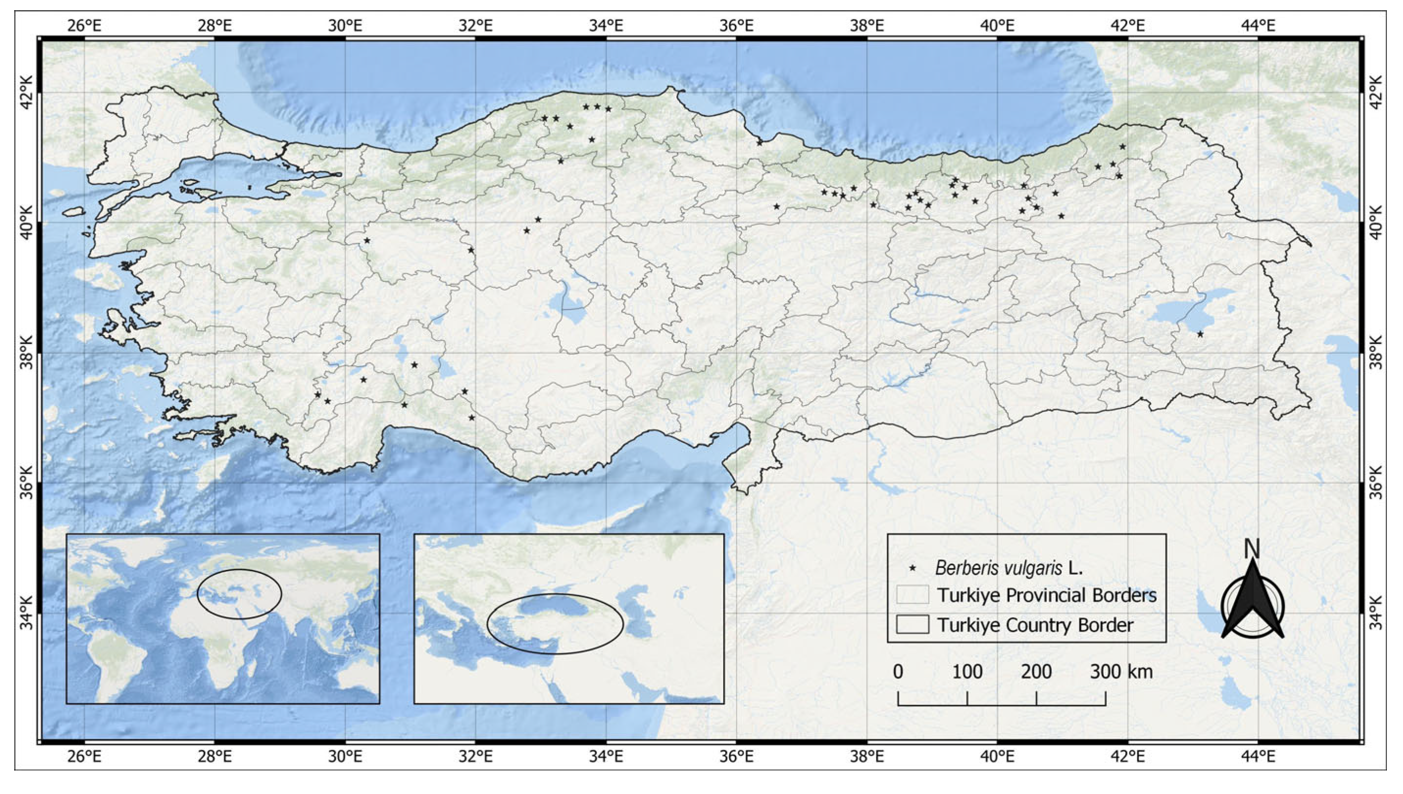
2.1. Study Region and Occurrence Data

The coordinate information for 50 points, called presence data and representing the natural geographical distribution area of Berberis vulgaris, was determined using the Biodiversity and Non-Wood Forest Products Database, Flora of Turkey, Global Biodiversity Information System (GBIF), and other literature sources [42,43,44,45], and converted into a “csv” format file that can be used by the MaxEnt program.
The coordinates of these points were marked in the WGS84 coordinate system in the current version of the QGIS program, utilizing Google Earth Satellite 5 m resolution base maps as the base data (Figure 1).
Descriptive information about the sample points, like coordinates, provinces, altitude, and climatic parameters is given in Table 1.

2.2. Bioclimatic Variables and Modeling

The coordinates obtained in the WGS 84 coordinate system were marked using the 5 m high spatial resolution Google Satellite Hybrid base maps, which are readily accessible in the 3.10.4 QGIS [46] program, the current version of QGIS (Quantum GIS).
Descriptive information (elevation, aspect, slope, temperature, precipitation, humidity, and insolation) for the sample points was determined with the help of maps obtained from the database [47]. The WorldClim database was used for predictive modeling of the current potential distribution area and future distribution area. WorldClim version 2.1 [47] includes monthly climate data encompassing minimum, average, and maximum temperature, precipitation, solar radiation, wind speed, water vapor pressure, and total precipitation from 1970 to 2000. Bioclimatic variables, with a spatial resolution of 2.5 min (approximately 20 km2), were used to determine the current distribution, and were derived from observed data in WorldClim version 2.1. The specific variables are detailed in Table 2 [47,48,49].
The IPSL-CM6A-LR was used to predict the species’ future distribution area. This model is also closer to the climate conditions of Türkiye. A series of new scenarios developed for CMIP6 in order to provide a broader future forecast in the sixth Assessment Report of the Intergovernmental Panel on Climate Change (IPCC6) were used in the study. The IPCC AR5 incorporates four representative concentration pathways (RCPs) that explore various potential future greenhouse gas emissions, namely RCP2.6, RCP4.5, RCP6.0, and RCP8.5. In CMIP6, these scenarios are revised and presented as shared socio-economic pathways (SSPs), specifically SSP1-2.6, SSP2-4.5, SSP4-6.0, and SSP5-8.5.
The SSP2 4.5 and SSP5 8.5 scenarios were used in this study. SSP2 4.5 is characterized as a scenario depicting moderate development and efforts to mitigate climate change. In contrast, SSP5 8.5 represents a high-development, high-emission pathway among the SSPs (socioeconomic pathways) published by CMIP6 [50]. These scenarios serve as crucial tools for climate scientists and policymakers, enabling them to examine the potential consequences of various socioeconomic and emissions trajectories on the Earth’s climate and ecosystems. The year periods 2041–2060 and 2081–2100 were used for both scenarios.
Before running the MaxEnt program, the digital elevation model (DEM), which includes bioclimatic variables and elevation data in raster data format to be used for present and future predictions, was transformed and cut within the boundaries determined as the working area with the cutting and conversion tools in the QGIS 3.16.1 program and converted to a file format with the “.asc” extension. In order to increase the predictive power of the model and solve the multicollinearity problem, Pearson’s correlation analysis was performed using the bioclimatic variables of the sample points in the SPSS 25 statistical package program. It was decided to reserve 25% of the sample points for testing and to print the prediction data used in the background. In order to determine which variable affected the gain alone or when removed, the jackknife test was used and linear, quadratic and hinge features were selected since the number of points was 50. Other settings were left as default. The program was run sequentially for the periods specified in the model’s scenarios, and model outputs for the present and the future were obtained in the “.asc” file format.
In the MaxEnt model, the presence of a species in an area is represented by a value ranging from 0 to 1. As the values approach 1, the probability or likelihood of the species being present in that area increases. Using the QGIS 3.16.1 program, all raster data were first converted to vector data with the raster calculation tool and then with the raster/vector conversion function. During the conversion, the threshold values for DN (digital number), called the fitness value, were classified as 0 = 0, 0–0.4 = 1, 0.4–0.8 = 2, and 0.8–1 = 3. In the current and future potential distribution maps, the threshold value classification for the distribution area was named as 0 “unsuitable”, 1 “less suitable”, 2 “suitable”, and 3 “very suitable”, and according to this classification, the current and future estimated distribution areas were calculated in km2.
In the last stage, change analysis was employed to ascertain the direction and magnitude of the change between the current and future estimated distribution areas of the species. To determine these changes, the intersection function was applied to the present and future forecast data in vector format across all time intervals.
Areas with suitability values (DN) of 0–0 in the attribute information of the data resulting from the intersection were not suitable; those that remained at the same value were considered “no change”; values that moved to a higher class were considered “gain”; values that moved to a lower class were considered “loss”; and the areas they covered were calculated in km2. Change maps were created by comparing the codes of today’s suitability classes and the codes on the maps determined according to future scenarios. The direction and magnitude of the changes were calculated according to the estimated distribution areas.
The overall methodological flowchart for this paper is shown in Figure 2. The flowchart comprises four main steps: (1) preparing and pre-processing the environmental variables; (2) assessing crucial factors and predicting potential distribution using MaxEnt models under various climate scenarios; (3) validating the distribution through field investigations and statistical methods; (4) analysis of the characteristics of the range shift for Berberis vulgaris.

3. Results

Pearson correlation tests were performed for 19 bioclimatic variables. In order to determine the potential distribution of Berberis vulgaris L. under current conditions, according to the Pearson correlation test results, variables with an r value of ±0.8 in the correlation matrix were excluded, 10 variables were excluded according to their importance among themselves, and “Mean Diurnal Range (BIO2)” was used as a variable that increased the predictive ability of the model. “Isothermality (BIO3)”; “Temperature Seasonality (BIO4)”; “Mean Temperature of Wettest Quarter (BIO8)”; “Mean Temperature of Driest Quarter (BIO9)”; “Mean Temperature of Coldest Quarter (BIO11)”; “Annual Precipitation (BIO12)”; “Precipitation of Driest Quarter (BIO17)”; and “Precipitation of Coldest Quarter (BIO19)” were selected as nine variables (Figure 3).
To determine the performance of the model, the area under the curve (AUC) value obtained from the Receiver Operating Characteristic (ROC) analysis and the output of the MaxEnt program was used. The AUC value for the training data was calculated as 0.904 and for the test data as 0.780. This value obtained for the training data shows that the model has a much higher descriptive predictive power than random guessing (Figure 4). Models with values above 0.75 are considered potentially useful [51].
The jackknife test option in the MaxEnt program was utilized to assess the impacts of environmental variables. This option enabled us to determine the significance of each independent variable in model creation [19,52,53,54,55].
According to the jackknife test results, the environmental variables with the highest gain when used in isolation were “Precipitation of Driest Quarter (BIO17)”; “Mean Temperature of Coldest Quarter (BIO11)”; “average temperature of the driest season (BIO9)”; and “Mean Diurnal Range (BIO2)” (Figure 5). Therefore, the jackknife test was considered to have the most useful information for the model.
The estimated current and future distribution maps of Berberis vulgaris are presented in Figure 6, Figure 7 and Figure 8. The current and future spatial distribution of the species, categorized based on suitability classes in these maps, are summarized in Table 3. In the MaxEnt model, the occurrence rate of a species in the area is determined by a value between 0 and 1. The produced model was classified and mapped at four different levels of suitability: not suitable (0), less suitable (0–0.5), suitable (0.5–0.75), and very suitable (0.75–1). The current spatial distribution of B. vulgaris can be observed in the maps obtained (Figure 6). There is a high correlation with the points representing B. vulgaris, which is distributed in the Mediterranean and the central and eastern Black Sea regions, and it can be seen that the very suitable areas (0.75–1) comprise 45,413.82 km2 (Table 3). However, when the SSP2 4.5 scenario was considered for the period 2041–2060 (Figure 7), the areas most suitable for B. vulgaris species comprised 59,120.05 km2. In the SSP2 4.5 scenario, very suitable areas were found to encompass 56,730.46 km2 in the 2081–2100 period.
Considering the SSP5 8.5 scenario for the period 2041–2060, the areas most suitable for Berberis vulgaris species comprised 66,670.39 km2. In the SSP5 8.5 scenario, very suitable areas were found to encompass 20,108.29 km2 in the 2081–2100 period (Figure 8). According to the model, the future distribution areas of B. vulgaris will be very interesting. In terms of geographical distribution, very suitable areas increased in the 2041–2060 and 2081–2100 periods of the SSP2 4.5 scenario and in the 2041–2060 period of the SSP5 8.5 scenario. In the SSP5 8.5 scenario, it can be seen that very suitable areas decreased in the 2081–2100 period (Table 3).
It is valuable to understand the differences between less suitable, suitable, and very suitable habitat classes. To elucidate these distinctions, the outcomes of the comparative change analysis (loss and gain) between the current distribution and the areas in the model with the predicted distributions are presented in Table 4. Additionally, the change maps can be observed in Figure 8 and Figure 9. According to the change analysis results given in Table 4, while the SSP2 4.5 scenario calculated an area gain of 81,463.731 km2 in the 2041–2060 time period, a loss of 168,278.165 km2 was also shown. In the SSP2 4.5 scenario for the 2081–2100 period, area gains were calculated as 80,263.758 km2 and area losses were calculated as 169,765.384 km2. In the SSP5 8.5 scenario, an area gain of 84,300.667 km2 was calculated in the 2041–2060 time period, while an area of 153,488.538 km2 was calculated as a loss (Figure 9).
In the SSP5 8.5 scenario, area gains were calculated as 37,092.284 km2 and lost areas were calculated as 196,525.05 km2 in the 2081–2100 periods (Figure 10).
Habitat change appears to be significant in the central and eastern Black Sea region of Türkiye. Several assessments suggest that certain species may migrate north, while some endemic species may face the risk of disappearing. Many studies investigating the effects of climate change on various species have consistently shown that climate has a significant impact on geographic distribution ranges. The results emphasize that climate change is poised to exert substantial effects on the ecosystem of the Black Sea region.

4. Discussion

According to the model, in terms of the geographical distribution of Berberis vulgaris L., very suitable areas increased in the SSP2 4.5 scenario for the 2041–2060 and 2081–2100 periods and in the SSP5 8.5 scenario for the 2041–2060 period. In the SSP5 8.5 scenario, it can be seen that very suitable areas decreased in the 2081–2100 period. It was predicted that the geographical distribution of B. vulgaris will decrease in the central Black Sea region and retreat to the eastern Black Sea and eastern Anatolia regions, and its distribution areas will increase. The conclusion drawn is that, with the rise in temperature due to climate change, Berberis vulgaris is likely to migrate toward higher and cooler altitudes. This shows that the species with increased habitat suitability will be resistant to the negative effects of climate change in the future.
In recent years, machine learning-based landslide susceptibility mapping has demonstrated significant success in applications related to landslide risk management. Ma et al. [56] introduced a new paradigm for end-to-end machine learning modeling, which was applied in landslide susceptibility mapping in the Three Gorges Reservoir Area (TGRA). Automated machine learning served as the backend model support for this paradigm. A carefully curated database, comprising data from 290 landslides and 11 conditioning factors, was gathered to implement automated machine learning and compare its performance with classically trained machine learning approaches. The experimental results indicate that automated machine learning provides an attractive alternative to manual machine learning, especially for practitioners with little expert knowledge in machine learning, by delivering a high-performance off-the-shelf solution for machine learning model development for landslide susceptibility mapping.
Liu et al. [57] introduced an earthworm optimization algorithm-optimized support vector regression for the accurate prediction of reservoir landslide displacement. The proposed approach underwent evaluation and comparison with various metaheuristics, such as an artificial bee colony, biogeography-based optimization, a genetic algorithm, gray wolf optimization, particle swarm optimization, and a water cycle algorithm, through the Friedman and post hoc Nemenyi tests. The experimental results from the Baishuihe landslide indicate that the earthworm optimization algorithm-optimized support vector regression is promising for accurate and reliable prediction of reservoir landslide displacements, thus aiding in medium- and long-term early landslide warnings.
Gao et al. [58] devised a neuro-fuzzy-based machine learning method to forecast the multiaxial fatigue life of diverse metallic materials. Their study involved validating the predictive performance of the proposed model using fatigue experimental data for six materials from the published literature. The results suggest that the proposed model can effectively predict the fatigue life of various materials under different loading paths.
Tuttu et al. [59] used the ~2050 and ~2090 periods of the IPSL CM6A-LR climate model SSP2 4.5 and SSP5 8.5 scenarios. They stated that the distribution of Crataegus × bornmuelleri will not be affected much by the changing climatic conditions in the coming years and will direct its distribution slightly toward the north of Türkiye.
Ngarega et al. [60] modeled the distribution of Colophosperpum mopane in South Africa according to climate change scenarios. The ~2050 and ~2070 periods of the RCP2.6, RCP4.5 and RCP8.5 scenarios were used for calculating future distribution areas. They observed that C. mopane is distributed across a total area of 1,281.242 km2 in Southern Africa, from Southern Angola and Northern Namibia to Central-South Mozambique. As a result of the model, they state that in climate change scenarios, suitable habitat areas will decrease significantly at the northern borders of potential distribution areas, while they will expand at the southern borders, and in general, they mentioned that suitable distribution areas would be minimized according to the RCP8.5 scenario, which was evaluated as strict. Martin et al. [61] concluded that Schinus terebinthifolia, which was brought to South Africa as an ornamental plant in the early 1900s, has expanded its distribution area. They state that Brazilian pepper has not yet reached its full potential distribution in South Africa and that the plant may spread to South Africa’s Western Cape Province.
Li et al. [62] modeled the spread of Sapindus mukorossi due to climate change on a global scale, and the model output indicated decreases in distribution, with the loss of all suitable habitats in Southwest Europe, North Africa, and West Asia. They state that new suitable habitats have emerged in the Southern Hemisphere, such as South America, Southern Africa, and Eastern Oceania. Li et al. [63] modeled the distribution areas of Robinia pseudoacacia with MaxEnt. They state that the primary suitable areas in the global potential distribution of Robinia pseudoacacia are concentrated mainly in the eastern United States, Europe, Australia, and New Zealand. In contrast, moderately suitable areas are predominantly located in China, Japan, South Africa, Chile, and Argentina.
As stated in these similar studies, each species has its own requirements to carry out its vital activities and shapes its living space accordingly. While some species cannot adapt to change and become narrow in their habitat or become extinct, some species continue their life activities with a tendency to move to northern and upper altitudes. Some of these may become invasive species. The modeling of species distribution has evolved into a crucial tool in various fields, including conservation, ecology, biogeography, evolution, invasive species control, and wildlife management studies [64,65,66,67].

5. Conclusions

Habitat changes due to future climate conditions require appropriate adaptation strategies to protect areas where threatened species may potentially occur [68]. Careful consideration should be given to the potential positive and negative effects of climate change, viewing them as an opportunity to implement suitable adaptation strategies. The potential expansion of suitable habitats for certain species could aid in their resilience against various pressures arising from climate change [69]. Conversely, species with low adaptation resistance will face the danger of extinction [70]. As a result, this study determined the areas and conditions in which Berberis vulgaris L. can maintain its ability to reproduce within the population––that is, areas with ecological niche potential––in order to survive and continue its existence.
Additionally, populations and genotypes of Berberis vulgaris that are resilient to future drought conditions due to climate change, which holds both ecological and economic value, should be identified through scientific research. In situ and ex situ genetic conservation areas should be designated and seed banks established. Initiating adaptation studies with genetic materials from different origins, especially in areas where the species is likely to expand in the future, will be a crucial approach for the sustainability and conservation strategy of Berberis vulgaris.

Author Contributions

Investigation, A.G.S. and A.U.; data curation and writing—original draft preparation, A.G.S.; writing—review and editing, A.G.S. and A.U. All authors have read and agreed to the published version of the manuscript.

Funding

This research received no external funding.

Institutional Review Board Statement

Not applicable.

Informed Consent Statement

Not applicable.

Data Availability Statement

The data presented in this study are available on request from the corresponding author.

Acknowledgments

The second author, Almira Uzun, is a scholar in the field of “Sustainable Forestry and Forest Disasters” within the scope of the YÖK 100/2000 project.

Conflicts of Interest

The authors declare no conflicts of interest.

References

  1. Adhikari, D.; Barik, S.; Upadhaya, K. Habitat distribution modelling for reintroduction of Ilex khasiana Purk., a critically endangered tree species of northeastern India. Ecol. Eng. 2012, 40, 37–43. [Google Scholar] [CrossRef]
  2. Barnosky, A.D.; Matzke, N.; Tomiya, S.; Wogan, G.O.; Swartz, B.; Quental, T.B.; Marshall, C.; McGuire, J.L.; Lindsey, E.L.; Maguire, K.C. Has the Earth’s sixth mass extinction already arrived? Nature 2011, 471, 51–57. [Google Scholar] [CrossRef]
  3. Uzun, A.; Orucu, O.K. Prediction of present and future spread of Adenocarpus complicatus (L.) Gay species according to climate variables. Turk. J. For. 2020, 21, 498–508. [Google Scholar] [CrossRef]
  4. United Nations Convention to Combat Desertification (Secretariat). United Naions Convention to Combat Desertification in Those Countries Experiencing Serious Drought and/or Desertification, Particulary in Africa; United Nations: New York, NY, USA, 1999. [Google Scholar]
  5. Arslan, E.S.; Gülçin, D.; Sarikaya, A.G.; Olmez, Z.; Gulcu, S.; Sen, I.; Orucu, O.K. Modeling of the current and future potential distribution of Stinking juniper (Juniperus foetidissima Willd.) with machine learning techniques. Eur. J. Sci. Technol. 2021, 22, 1–12. [Google Scholar]
  6. Chakraborty, A.; Joshi, P.; Sachdeva, K. Predicting distribution of major forest tree species to potential impacts of climate change in the central Himalayan region. Ecol. Eng. 2016, 97, 593–609. [Google Scholar] [CrossRef]
  7. Zhao, H.; Zhang, H.; Xu, C. Study on Taiwania cryptomerioides under climate change: MaxEnt modeling for predicting the potential geographical distribution. Glob. Ecol. Conserv. 2020, 24, e01313. [Google Scholar] [CrossRef]
  8. Atefi, M.; Ghavami, A.; Hadi, A.; Askari, G. The effect of barberry (Berberis vulgaris L.) supplementation on blood pressure: A systematic review and meta-analysis of the randomized controlled trials. Complement. Ther. Med. 2021, 56, 102608. [Google Scholar] [CrossRef] [PubMed]
  9. Maliwichi-Nyirenda, C.P.; Maliwichi, L.L.; Franco, M. Medicinal uses of Berberis holstii Engl. (Berberidaceae) in Malawi, the only African endemic barberry. J. Med. Plants Res. 2011, 5, 1367–1373. [Google Scholar]
  10. Ayna, O.F.; Arslanoglu, S.F. The Types of Berberis Growing in Anatolian Geography and Traditional Uses. Int. J. Life Sci. Biotechnol. 2019, 2, 36–42. [Google Scholar] [CrossRef]
  11. Mozaffarian, V. A Dictionary of Iranian Plant Names; Farhang Moaser: Tehran, Iran, 1996; pp. 396–398. [Google Scholar]
  12. Attuluri, M.L.V.S.; Darwin, R.C. Drug Bioavailability, Stability and Anticancer Effect of Berberine-loaded Magnetic Nanoparticles on MDA-MB-231 Cells in Breast Cancer. Indian J. Pharm. Educ. Res. 2022, 56, S444–S453. [Google Scholar] [CrossRef]
  13. Cansaran, A.; Kaya, O.F.; Yildirim, C. An Ethnobotanical Study (Amasya/Gümüşhacıköy) Between the Vicinity of Ovabaşı, Akpınar, Güllüce and Köseler Villages. Sci. Eng. J. Fırat. Univ. 2007, 19, 243–257. [Google Scholar]
  14. Kayacık, H. Special Systematics of Forest and Park Trees; Istanbul University Faculty of Forestry Publications: Istanbul, Turkey, 1968. [Google Scholar]
  15. Komarov, V.; Schischkin, B. Flora of the USSR Volume VII, Scientific Academy of the U.S.S.R. Leningrad: Moscow, Russia, 1937.
  16. Korkmaz, M.; Alpaslan, Z. Ethnobotanical properties of Ergan Mountain (Erzincan-Turkey). Bağbahçe Sci. J. 2014, 1, 1–31. [Google Scholar]
  17. Nandi, A.; Pal, A.K. Interpreting Machine Learning Models: Learn Model Interpretability and Explainability Methods; Apress: Berkeley, CA, USA, 2022. [Google Scholar]
  18. Jiang, H. Machine Learning Fundamentals: A Concise Introduction; Cambridge University Press: Cambridge, UK, 2021. [Google Scholar]
  19. Eker, R.; Alkis, K.C.; Ucar, Z.; Aydın, A. Using Machine Learning in Forestry. Turk. J. For. 2023, 24, 150–177. [Google Scholar] [CrossRef]
  20. Bishop, C.M. Model-based machine learning. Philos. Trans. R. Soc. A Math. Phys. Eng. Sci. 2013, 371, 20120222. [Google Scholar] [CrossRef]
  21. Zhang, J.; Li, S. A Review of Machine Learning Based Species’ Distribution Modelling. In Proceedings of the 2017 International Conference on Industrial Informatics—Computing Technology, Intelligent Technology, Industrial Information Integration (ICIICII), Wuhan, China, 2–3 December 2017; p. 199. [Google Scholar] [CrossRef]
  22. Mitchell, T.M. Machine Learning; McGraw-Hill: New York, NY, USA, 1997. [Google Scholar]
  23. Scherrer, D.; Guisan, A. Ecological indicator values reveal missing predictors of species distributions. Sci. Rep. 2019, 9, 3061. [Google Scholar] [CrossRef]
  24. Elith, J.; Phillips, S.J.; Hastie, T.; Dudik, M.; Chee, Y.E.; Yates, C.J. A statistical explanation of MaxEnt for ecologists. Divers. Distrib. 2011, 17, 43–57. [Google Scholar] [CrossRef]
  25. Feng, X.; Park, D.S.; Walker, C.; Peterson, A.T.; Merow, C.; Papeş, M. A checklist for maximizing reproducibility of ecological niche models. Nat. Ecol. Evol. 2019, 3, 1382–1395. [Google Scholar] [CrossRef]
  26. Peterson, A.T.; Papes, M.; Eaton, M. Transferability and model evaluation in ecological niche modeling: A comparison of GARP and Maxent. Ecography 2007, 30, 550–560. [Google Scholar] [CrossRef]
  27. Arslan, E.S. Evaluation of urban road trees in terms of ecosystem services according to climate change scenarios and species distribution model: The case of Robinia pseudoacacia L. Turk. J. For. 2019, 20, 142–148. [Google Scholar] [CrossRef]
  28. Phillips, S.J.; Dudík, M. Modeling of species distributions with Maxent: New extensions and a comprehensive evaluation. Ecography 2008, 31, 161–175. [Google Scholar] [CrossRef]
  29. Sarikaya, O.; Karaceylan, I.; Sen, I. Maximum entropy modeling (maxent) of current and future distributions of Ips mannsfeldi (Wachtl, 1879)(Curculionidae: Scolytinae) in Turkey. Appl. Ecol. Environ. Res. 2018, 16, 2527–2535. [Google Scholar] [CrossRef]
  30. Sérgio, C.; Figueira, R.; Draper, D.; Menezes, R.; Sousa, A.J. Modelling bryophyte distribution based on ecological information for extent of occurrence assessment. Biol. Conserv. 2007, 135, 341–351. [Google Scholar] [CrossRef]
  31. Tittensor, D.P.; Baco, A.R.; Brewin, P.E.; Clark, M.R.; Consalvey, M.; Hall-Spencer, J.; Rowden, A.A.; Schlacher, T.; Stocks, K.I.; Rogers, A.D. Predicting global habitat suitability for stony corals on seamounts. J. Biogeogr. 2009, 36, 1111–1128. [Google Scholar] [CrossRef]
  32. Wang, Y.S.; Xie, B.Y.; Wan, F.H.; Xiao, Q.M.; Dai, L.Y. The potential geographic distribution of Radopholus similis in China. Agric. Sci. China 2007, 6, 1444–1449. [Google Scholar] [CrossRef]
  33. Ward, D.F. Modelling the potential geographic distribution of invasive ant species in New Zealand. Biol. Invasions 2007, 9, 723–735. [Google Scholar] [CrossRef]
  34. Williams, J.N.; Seo, C.; Thorne, J.; Nelson, J.K.; Erwin, S.; O’Brien, J.M.; Schwartz, M.W. Using species distribution models to predict new occurrences for rare plants. Divers. Distrib. 2009, 15, 565–576. [Google Scholar] [CrossRef]
  35. Wollan, A.K.; Bakkestuen, V.; Kauserud, H.; Gulden, G.; Halvorsen, R. Modelling and predicting fungal distribution patterns using herbarium data. J. Biogeogr. 2008, 35, 2298–2310. [Google Scholar] [CrossRef]
  36. Yuan, H.S.; Wei, Y.L.; Wang, X.G. Maxent modeling for predicting the potential distribution of Sanghuang, an important group of medicinal fungi in China. Fungal Ecol. 2015, 17, 140–145. [Google Scholar] [CrossRef]
  37. Li, G.; Huang, J.; Guo, H.; Du, S. Projecting species loss and turnover under climate change for 111 Chinese tree species. For. Ecol. Manag. 2020, 477, 118488. [Google Scholar] [CrossRef]
  38. Pearson, R.G.; Raxworthy, C.J.; Nakamura, M.; Peterson, A.T. Predicting species distributions from small numbers of occurrence records: A test case using cryptic geckos in Madagascar. J. Biogeogr. 2007, 34, 102–117. [Google Scholar] [CrossRef]
  39. Phillips, S.J.; Anderson, R.P.; Schapire, R.E. Maximum Entropy Modeling of Species Geographic Distributions. Ecol. Model. 2006, 190, 231–259. [Google Scholar] [CrossRef]
  40. Yi, Y.; Cheng, X.; Yang, Z.; Wieprecht, S.; Zhang, S.; Wu, Y. Evaluating the ecological infuence of hydraulic projects: A review of aquatic habitat suitability models. Renew. Sustain. Energy Rev. 2017, 68, 748–762. [Google Scholar] [CrossRef]
  41. Whittemore, A. Berberis; Flora of North America: St. Louis, MO, USA, 1997; Volume 3, pp. 276–286. [Google Scholar]
  42. Ministry of Agriculture and Forestry General Directorate of Forestry. BIYOD Biodiversity and Non-Wood Forest Products Database; Ministry of Agriculture and Forestry General Directorate of Forestry: Yenimahalle, Türkiye, 2020.
  43. Davis, P.H. Flora of Turkey the East Aegean Islands; Edinburgh University Press: Edinburgh, UK, 1965; Volume 1. [Google Scholar]
  44. GBIF. GBIF Occurrence Download. 2023. Available online: https://www.gbif.org/occurrence/download/0026674-231120084113126 (accessed on 9 November 2023).
  45. Akkemik, U. All Trees and Shrubs of Turkey; Türkiye İş Bank Publications: Istanbul, Türkiye, 2020. [Google Scholar]
  46. QGIS. QGIS 3.10.4 Coruna—A Free and Open GIS. Available online: https://www.qgis.org/en/site/forusers/visualchangelog322/index.html (accessed on 15 November 2023).
  47. WorldClim. WorldClim—Global Climate Data. 2019. Available online: www.worldclim.org (accessed on 7 November 2023).
  48. Fick, S.E.; Hijmans, R.J. WorldClim 2: New 1-km Spatial Resolution Climate Surfaces for Global Land Areas. Int. J. Climatol. 2017, 37, 4302–4315. [Google Scholar] [CrossRef]
  49. Hijmans, R.J.; Cameron, S.E.; Parra, J.L.; Jones, P.G.; Jarvis, A. Very high resolution interpolated climate surfaces for global land areas. Int. J. Climatol. A J. R. Meteorol. Soc. 2005, 25, 1965–1978. [Google Scholar] [CrossRef]
  50. Hausfather, Z.; Drake, H.F.; Abbott, T.; Schmidt, G.A. Evaluating the performance of past climate model projections. Geophys. Res. Lett. 2020, 47, e2019GL085378. [Google Scholar] [CrossRef]
  51. Husband, B.C. Review of Quantitative Methods for Conservation Biology. In The Quarterly Review of Biology; Ferson, S., Burgman, M., Eds.; Springer: New York, NY, USA, 2002; Volume 77, pp. 94–165. [Google Scholar]
  52. Fielding, A.H.; Bell, J.F. A review of methods for assessment of prediction errors in conservation presence/absence models. Environ. Conserv. 1997, 24, 38–49. [Google Scholar] [CrossRef]
  53. Hundessa, S.; Li, S.; Liu, D.L.; Guo, J.; Guo, Y.; Zhang, W.; Williams, G. Projecting environmental suitable areas for malaria transmission in China under climate change scenarios. Environ. Res. 2018, 162, 203–210. [Google Scholar] [CrossRef]
  54. Khanum, R.; Mumtaz, A.S.; Kumar, S. Predicting impacts of climate change on medicinal asclepiads of Pakistan using Maxent modeling. Acta Oecologica 2013, 49, 23–31. [Google Scholar] [CrossRef]
  55. Shcheglovitova, M.; Anderson, R.P. Estimating optimal complexity for ecological niche models: A jack knife approach for species with small sample sizes. Eco Log. Model. 2013, 269, 9–17. [Google Scholar] [CrossRef]
  56. Ma, J.; Lei, D.; Ren, Z.; Tan, C.; Xia, D.; Guo, H. Automated Machine Learning-Based Landslide Susceptibility Mapping for the Three Gorges Reservoir Area, China. Math. Geosci. 2023. [Google Scholar] [CrossRef]
  57. Liu, Z.; Ma, J.; Xia, D.; Jiang, S.; Ren, Z.; Tan, C.; Lei, D.; Guo, H. Toward the reliable prediction of reservoir landslide displacement using earthworm optimization algorithm-optimized support vector regression (EOA-SVR). Nat. Hazards 2023. [Google Scholar] [CrossRef]
  58. Gao, J.; Heng, F.; Yuan, Y.; Liu, Y. A novel machine learning method for multiaxial fatigue life prediction: Improved adaptive neuro-fuzzy inference system. Int. J. Fatigue 2024, 178, 108007. [Google Scholar] [CrossRef]
  59. Tuttu, G.; Aytas, I.; Bulut, S. Estimation of the distribution areas of Crataegus× bornmuelleri Zabel ex KI Chr. & Ziel. depending on climate change. In Proceedings of the International Eurasia Climate Change Congress, Van, Türkiye, 29 September–1 October 2022; Van Yuzuncu Yil University Press Publication: Van, Türkiye, 2022; p. 53. [Google Scholar]
  60. Ngarega, B.K.; Masocha, V.F.; Schneider, H. Forecasting the effects of bioclimatic characteristics and climate change on the potential distribution of Colophospermum mopane in southern Africa using Maximum Entropy (Maxent). Ecol. Inform. 2021, 65, 101419. [Google Scholar] [CrossRef]
  61. Martin, G.; Magengelele, N.L.; Paterson, I.D.; Sutton, G.F. Climate modelling suggests a review of the legal status of Brazilian pepper Schinus terebinthifolia in South Africa is required. South Afr. J. Bot. 2020, 132, 95–102. [Google Scholar] [CrossRef]
  62. Li, Y.; Shao, W.; Jiang, J. Predicting the potential global distribution of Sapindus mukorossi under climate change based on MaxEnt modelling. Environ. Sci. Pollut. Res. 2022, 29, 21751–21768. [Google Scholar] [CrossRef] [PubMed]
  63. Li, G.; Xu, G.; Guo, K.; Du, S. Mapping the Global Potential Geographical Distribution of Black Locust (Robinia pseudoacacia L.) Using Herbarium Data and a Maximum Entropy Model. Forests 2014, 5, 2773. [Google Scholar] [CrossRef]
  64. Barve, N.; Barve, V.; Jiménez-Valverde, A.; Lira-Noriega, A.; Maher, S.P.; Peterson, A.T.; Soberón, J.; Villalobos, F. The crucial role of the accessible area in ecological niche modeling and species distribution modeling. Ecol. Model. 2011, 222, 1810–1819. [Google Scholar] [CrossRef]
  65. Elith, J.; Graham, C.H.; Anderson, R.P.; Dudík, M.; Ferrier, S. Novel methods improve prediction of species’ distributions from occurrence data. Ecography 2006, 29, 129–151. [Google Scholar] [CrossRef]
  66. Kariyawasam, C.S.; Kumar, L.; Ratnayake, S.S. Invasive Plants Distribution Modeling: A Tool for Tropical Biodiversity Conservation With Special Reference to Sri Lanka. Trop. Conserv. Sci. 2019, 12, 1940082919864269. [Google Scholar] [CrossRef]
  67. Miller, J. Species Distribution Modeling. Geogr. Compass 2010, 4, 490–509. [Google Scholar] [CrossRef]
  68. Muller, J.J.; Nagel, L.M.; Palik, B.J. Forest adaptation strategies aimed at climate change: Assessing the performance of future climate-adapted tree species in a northern Minnesota pine ecosystem. For. Ecol. Manag. 2019, 451, 117539. [Google Scholar] [CrossRef]
  69. Moukrim, S.; Lahssini, S.; Rhazi, M.; Alaoui, H.M.; Benabou, A.; Wahby, I.; Rhazi, L. Climate change impacts on potential distribution of multipurpose agroforestry species: Argania spinosa (L.) Skeels as case study. Agrofor. Syst. 2019, 93, 1209–1219. [Google Scholar] [CrossRef]
  70. Wiens, J.J. Climate-Related Local Extinctions Are Already Widespread among Plant and Animal Species. PLoS Biol. 2016, 14, e2001104. [Google Scholar] [CrossRef] [PubMed]
Figure 1. Berberis vulgaris L. sample points.
Sustainability 16 01230 g001
Figure 2. Flowchart illustrating the methodology employed for MaxEnt modeling and forecasting the future potential distribution of Berberis vulgaris L. under climate change scenarios.
Sustainability 16 01230 g002
Figure 3. Bioclimatic variables selected for the model.
Sustainability 16 01230 g003
Figure 4. ROC curve of distribution model.
Sustainability 16 01230 g004
Figure 5. ROC curve of Berberis vulgaris L.
Sustainability 16 01230 g005
Figure 6. Estimated current distribution area of Berberis vulgaris L. (not suitable (1), less suitable (2), suitable (3), and very suitable (4)).
Sustainability 16 01230 g006
Figure 7. SSP2 4.5 scenario: (A) 2041–2061 period and (B) estimated distribution areas according to 2081–2100 period (not suitable (1), less suitable (2), suitable (3), and very suitable (4)).
Sustainability 16 01230 g007
Figure 8. SSP5 8.5 scenario: (A) 2041–2061 period and (B) estimated distribution areas according to 2081–2100 period (not suitable (1), less suitable (2), suitable (3), and very suitable (4)).
Sustainability 16 01230 g008
Figure 9. Change between the estimated current distribution area of Berberis vulgaris L. and the SSP2 4.5 scenario: (A) change between the estimated distribution area in the 2041–2060 period and (B) change between the estimated distribution area in the 2081–2100 period.
Sustainability 16 01230 g009
Figure 10. Change between estimated current distribution area of Berberis vulgaris L. and SSP5 8.5 scenario: (A) change between estimated distribution area in the 2041–2060 period and (B) change between estimated distribution area in the 2081–2100 period.
Sustainability 16 01230 g010
Table 1. Attribute information of sample points of Berberis vulgaris L.
Berberis vulgarisxyProvince-DistrictPrecipitation (mm)Temperature (°C)Altitude (m)
131.9279339.57613Eskişehir-Sivrihisar32.0833312.15833745
241.868640.71457Erzurum-Oltu41.083337.851315
341.7713940.89483Artvin-Yusufeli51.583337.551539
441.5422540.85444Artvin-Yusufeli64.5833411.83333730
537.7968240.52826Ordu-Mesudiye52.166677.833331329
633.4463841.47991Kastamonu-Daday50.583338.85922
732.9572640.04383Ankara-Altındağ33.5833311.18333991
840.8883740.45238Erzurum-İspir41.666678.866671358
933.6923541.7753Kastamonu-Küre57.416676.083331428
1037.5048640.44489Tokat-Reşadiye49.256.81503
1132.7835939.87803Ankara-Çankaya31.6666710.89167980
1239.6586840.32847Gümüşhane-Centre44.583335.208331819
1339.3050840.57435Gümüşhane-Torul47.5833310.725943
1437.3448840.46817Tokat-Reşadiye48.757.708331543
1539.3505940.4239Gümüşhane-Centre419.058331305
1633.8636141.77972Kastamonu-Devrekani56.583336.8751290
1733.7812141.27519Kastamonu-Centre44.166678.31107
1833.304240.94056Çankırı-Kurşunlu48.833336.533331285
1930.9070937.19898Antalya-Serik59.5833316.98333258
2029.5778137.35591Denizli-Acıpayam4611.691671054
2140.9800740.09898Erzurum-Aziziye43.166674.166671946
2230.3349539.72538Eskişehir-Tepebaşı38.6666710.86667905
2338.09740.27174Sivas-Suşehri49.4166710.133331204
2437.6283740.41298Tokat-Reşadiye495.941671602
2538.632540.22757Giresun-Alucra48.754.516671970
2638.6461540.4052Giresun-Şebinkarahisar48.258.351414
2738.8160140.34509Giresun-Alucra47.666676.216671753
2838.9397240.26588Giresun-Alucra46.333336.341671684
2930.2807937.58223Burdur-Centre44.0833310.708331271
3031.0610637.81084Isparta-Aksu50.3333310.233331247
3131.0617437.81049Isparta-Aksu50.3333310.233331247
3229.7298737.25625Burdur-Tefenni45.3333310.9251295
3334.0341541.74219Kastamonu-Devrekani55.833336.4251360
3433.2323641.59983Kastamonu-Azdavay567.7993
3540.3792240.17859Bayburt-Centre41.255.866671711
3640.599240.23474Bayburt-Centre50.753.0752145
3740.3792640.17865Bayburt-Centre41.255.866671711
3840.599240.23474Bayburt-Centre50.753.0752145
3940.4052240.57008Trabzon-Çaykara49.916674.583331900
4039.5023540.54477Gümüşhane-Torul44.756.658331552
4139.3576240.65752Gümüşhane-Torul48.756.451763
4231.8325237.40472Konya-Seydişehir54.8333311.141671127
4333.058341.60131Kastamonu-Pınarbaşı57.416679.33333770
4436.3530141.22309Samsun-Canik53.4166711.76667583
4536.6150340.24437Tokat-Centre38.666679.466671048
4640.4713840.37269Bayburt-Centre39.57.158331632
4741.9195141.16631Artvin-Ardanuç69.333349.741671414
4843.1097138.28423Van-Gevaş45.757.751951
4931.9400937.00053Antalya-Akseki58.758.516671960
5038.7468240.45486Giresun-Alucra51.254.366671937
Table 2. Bioclimatic variables [38].
Bio 1Annual Mean Temperature
Bio 2Mean Diurnal Range (Mean of Monthly (Max Temp.–Min Temp.)
Bio 3Isothermality (WC2/WC7) (×100)
Bio 4Temperature Seasonality (Standard Deviation × 100)
Bio 5Max Temperature of Warmest Month
Bio 6Min Temperature of Coldest Month
Bio 7Temperature Annual Range (WC5–WC6)
Bio 8Mean Temperature of Wettest Quarter
Bio 9Mean Temperature of Driest Quarter
Bio 10Mean Temperature of Warmest Quarter
Bio 11Mean Temperature of Coldest Quarter
Bio 12Annual Precipitation
Bio 13Precipitation of Wettest Month
Bio 14Precipitation of Driest Month
Bio 15Precipitation Seasonality (Coefficient of Variation)
Bio 16Precipitation of Wettest Quarter
Bio 17Precipitation of Driest Quarter
Bio 18Precipitation of Warmest Quarter
Bio 19Precipitation of Coldest Quarter
Table 3. Spatial representation of the potential geographical distribution of Berberis vulgaris L. for the years 2041–2060 and 2081–2100 under the current, SSP2 4.5, and SSP5 8.5 climate scenarios (km2).
SSP2 4.5SSP5 8.5
Current%2041–2060%2081–2100%2041–2060%2081–2100%
Not suitable566,141.972.65654,92584.04659,05084.57637,449.181.80725,712.193.13
Less suitable121,749.915.6239,944.765.1340,174.395.1648,162.236.1820,3182.61
Suitable45,963.455.9025,279.33.2423,314.312.9926,987.423.4613,130.711.68
Very suitable45,413.825.8359,120.057.5956,730.467.2866,670.398.5620,108.292.58
Total779,269.1100779,269.1100779,269.1100779,269.1100779,269.1100
Table 4. Change analysis of Berberis vulgaris L. (km2).
SSP2 4.5SSP5 8.5
Change2041–2060%2081–2100%2041–2060%2081–2100%
Gain81,463.73110.4580,263.75810.3084,300.66710.8237,092.2844.76
Loss168,278.16521.59169,765.38421.79153,488.53819.70196,525.0525.22
Stable18,751.6072.4117,535.7242.2530,563.1063.927300.5230.94
Unsuitable510,775.64265.55511,704.25965.66510,916.83665.5653,8351.2369.08
Total779,269.145100779,269.145100779,269.145100779,269.145100
Disclaimer/Publisher’s Note: The statements, opinions and data contained in all publications are solely those of the individual author(s) and contributor(s) and not of MDPI and/or the editor(s). MDPI and/or the editor(s) disclaim responsibility for any injury to people or property resulting from any ideas, methods, instructions or products referred to in the content.

