Soil Strength Parameters for the Sustainable Design of Unsupported Cuts Under Drained Conditions Using Reliability Analysis

Abstract

Unsupported excavations are frequently performed in several geological and geotechnical projects, particularly for constructing roads and railways, and they are often carried out in different materials. The design of such cuts in soils needs the determination of representative values of its mechanical properties, particularly of the strength parameters, and the application of adequate safety factors. The procedure should ensure a sustainable design of those cuts, allowing for economical solutions that guarantee a low probability of geological–geotechnical failure. This paper assesses the reliability of unsupported cuts in soils, under drained conditions, assuming a Mohr–Coulomb strength criterion. Statistical meshes are generated considering the spatial variability of the friction angle and of the true effective cohesion, which are assumed to be uncorrelated. In this process, typical values of the coefficients of variation and of the horizontal and vertical scales of fluctuation are applied. Soil characterisation is simulated in each statistical mesh, and the characteristic values of the strength parameters are determined using statistical methods. Unsupported cuts of different heights and inclinations are designed using typical safety factors. Slope stability analyses are carried out using Random Finite Element Limit Analysis. The uncertainty in the actions is considered, and the probability of failure is determined by direct reliability analysis. The results show the relevance of the ratio between the scale of fluctuation and the excavation depth, the slope inclination, and the characteristic value of the soil strength parameters on the probability of failure. Values of adequate safety factors are proposed towards obtaining an appropriate probability of failure, compatible with the sustainable design of the cuts.

1. Introduction

The construction of roads, railways, and other civil engineering projects involves the execution of unsupported excavations in different types of geotechnical materials, in several geological conditions. Some of these geotechnical works stretch over large distances, therefore significantly impacting the surroundings. The sustainable design of these cuts involves, among other concerns, considering the safety level depending on the structure’s importance. In fact, one of the United Nations’ Goals for Sustainable Development is Goal 11, “Make cities and human settlements inclusive, safe, resilient and sustainable”, and the subject of this paper is, in particular, related to the topics “Disaster risk reduction” and “Sustainable cities and human settlements”. This sustainable design should involve a certain minimum level of safety that should ensure an appropriate performance during the structures’ life, with an economical solution leading to a robust geotechnical project [1], but should also take into account that a too-high level of safety for the importance of the structure will certainly involve more resources than necessary.

This level of safety can be considered through a minimum probability of failure, and modern design codes aim to specify values of safety factors (usually partial safety factors) which have the goal of ensuring a certain probability of failure. More important structures should be designed considering lower probability of failure. For the unsupported cuts studied in this paper, a maximum probability of failure of around ${10}^{-4}$ is considered. This corresponds to a reliability index of 3.8 or higher, which is frequently considered in standards [2] and in the traditional design methods [3,4,5,6,7].

The design of unsupported cuts needs the choice of appropriate calculation models, strength parameters and safety factors. Good calculation models for unsupported cuts are available, and therefore, its design needs appropriate soil strength parameters, capable of adequately describing the strength of the material, and also appropriate values of the safety factors, allowing the sufficiently low desired probability of failure.

The appropriate soil strength parameters are their characteristic values, which should result from soil characterisation that should be as meticulous as possible [8,9,10]. Nevertheless, it is impossible to avoid uncertainties associated with the soil formation process (inherent), the measurement error, or transformation models (epistemic) [11,12,13,14]. For this reason, it is necessary to consider the effects of uncertainties when assessing the stability of unsupported cuts, as demonstrated in previous studies [15,16,17,18,19,20,21,22,23]. Some of these studies have shown that the spatial variability of soil shear strength parameters significantly influences the outcome of the reliability analysis of soil slopes and, in particular, they indicate that the probability of slope failure decreases as the scale of fluctuation reduces.

A few other contributions can be found in the literature considering spatial variability. They focus on the location of site investigation for slope stability [24,25,26,27]. These works assume an undrained soil behaviour and concluded that when considering a single site investigation operation, the crest seems to be the optimal location to execute it. No similar study considering drained conditions could be found in the literature.

Some authors [28,29,30,31] have investigated the measure to which the partial coefficients of the EN 1997-1 [2] guarantee the desired level of safety. In these studies, spatial variability was not considered. Their results indicate that the obtained safety level is mostly below the expected.

The results from these studies highlight the need for further research on the issue of obtaining the desired level of safety. Therefore, this paper aims to evaluate if current procedures for determining the characteristic values of soil strength parameters and values of safety factors currently used in codes and practices do ensure the desired minimum level of safety of unsupported cuts, and therefore, their sustainable design. The level of safety does not depend on the values of the safety factors alone, and they need to be analysed in conjunction with appropriate soil strength parameters. The determination of safety levels simultaneously considering the influence of partial coefficient values and the process of determining characteristic values is the main innovative contribution of this paper.

This is achieved through a procedure involving the determination of collapse loads using the software mechpy, developed within the authors’ team [32], which has previously been applied to reliability analyses of other geotechnical structures [33,34,35,36].

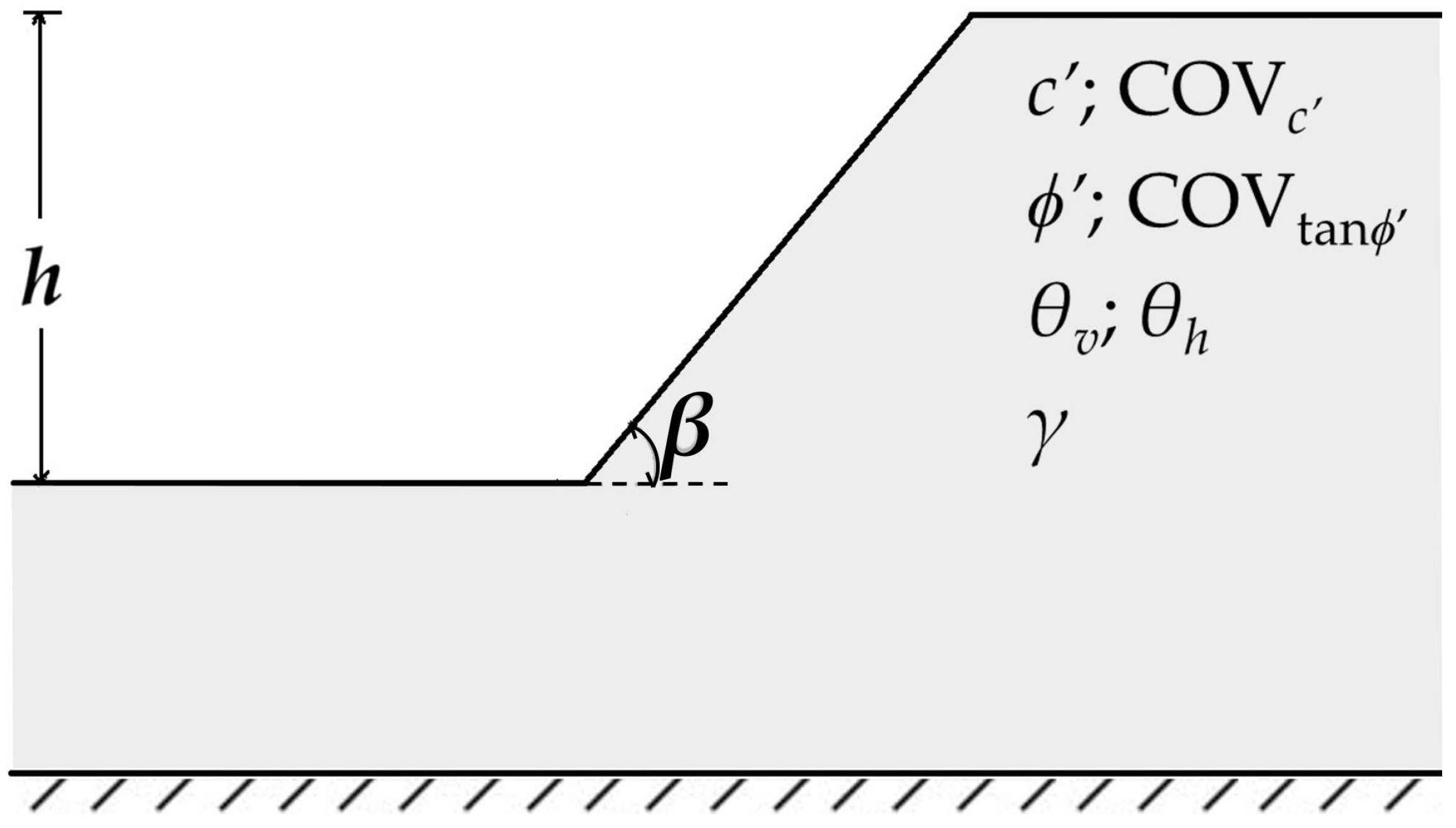
2. Description of the Unsupported Cut

The problem of the unsupported cut analysed in this article is shown in Figure 1. It has an excavation depth h and a constant inclination $\beta$. It is analysed under plane strain conditions. The unit weight causing collapse, $\gamma$, is, in this paper, determined by the finite element calculations. The phreatic level is assumed to be deep enough to not affect the stability of the slope. The shear strength of the soil is defined by the effective cohesion, c’, and the friction angle, ${\varphi }^{\prime }$. Therefore, the study considers drained conditions and the soil strength described by the Mohr–Coulomb criterion. The drained condition is, in most situations, the relevant case in unsupported excavation slopes.

The soil strength properties are described as random variables, modelled as random fields using the mean value, the coefficient of variation, COV, and the vertical and horizontal scales of fluctuation (${\theta }_v,{\theta }_h$). The scale of fluctuation is a measure of the distance within which the soil property shows a relatively strong correlation with itself [37]. In sedimentary soils, it is usually an anisotropic parameter, as the horizontal scale of fluctuation is typically significantly larger than the vertical scale of fluctuation [11,14].

The spatial correlation describes the correlation between the same property measured at different points [14]. It is expressed by the coefficient of correlation, $\rho$, computed by the vertical and the horizontal distance between the centre of mass of the elements in the statistical mesh, $\Delta y$ and $\Delta x$, and the scale of fluctuation. In this paper, $\rho$ is described by a two-dimensional ellipsoidal correlation function [38] expressed by

$$\rho (\Delta x,\Delta y)=exp\left[-2\sqrt{{\left({\displaystyle \frac{\Delta y}{{\theta }_v}}\right)}^2+{\left({\displaystyle \frac{\Delta x}{{\theta }_h}}\right)}^2}\right]$$

(1)

3. Methodology

3.1. Overview

The methodology followed in this work is summarised in Figure 2. A relatively large number of statistical meshes are generated, considering the spatial distribution of the effective cohesion and friction angle. These statistical meshes are samples that intend to simulate different spatial distributions of those soil strength parameters. Before the excavation is performed, the soil mass is considered to be divided into square elements. Within each element, the soil strength parameters are constant.

Characteristic values of these strength parameters are determined, using two different approaches, which will be detailed in Section 3.3. Using these characteristic strength parameters, the unsupported cuts are designed. The design usually involves specifying the geometry that verifies safety, but in this case, the geometry is assumed fixed. Therefore, by “design”, it is meant, in this case, determining the maximum value of the soil unit weight that verifies the safety of the unsupported cuts. In this work, this procedure uses Finite Element Limit Analysis (FELA) with the software mechpy, which is a finite element implementation of the upper- and lower-bound theorems of limit analysis, as described in Vicente da Silva et al.’s work [39]. At this stage, calculations involve considering homogeneous soil with the characteristic values of soil strength parameters mentioned above.

A finite element mesh with the geometry of the excavation is superposed to each statistical mesh, and the soil properties are mapped from the statistical elements to the finite elements. Random Finite Element Limit Analyses (RFELA), both upper- and lower-bound, are performed, also using mechpy. From each RFELA calculation, the unit weight causing collapse is determined. Comparing the values of the unit weight determined from “design” with those from RFELA, a reliability analysis is performed and the probability of failure is determined. The following sections describe each step of the framework in more detail.

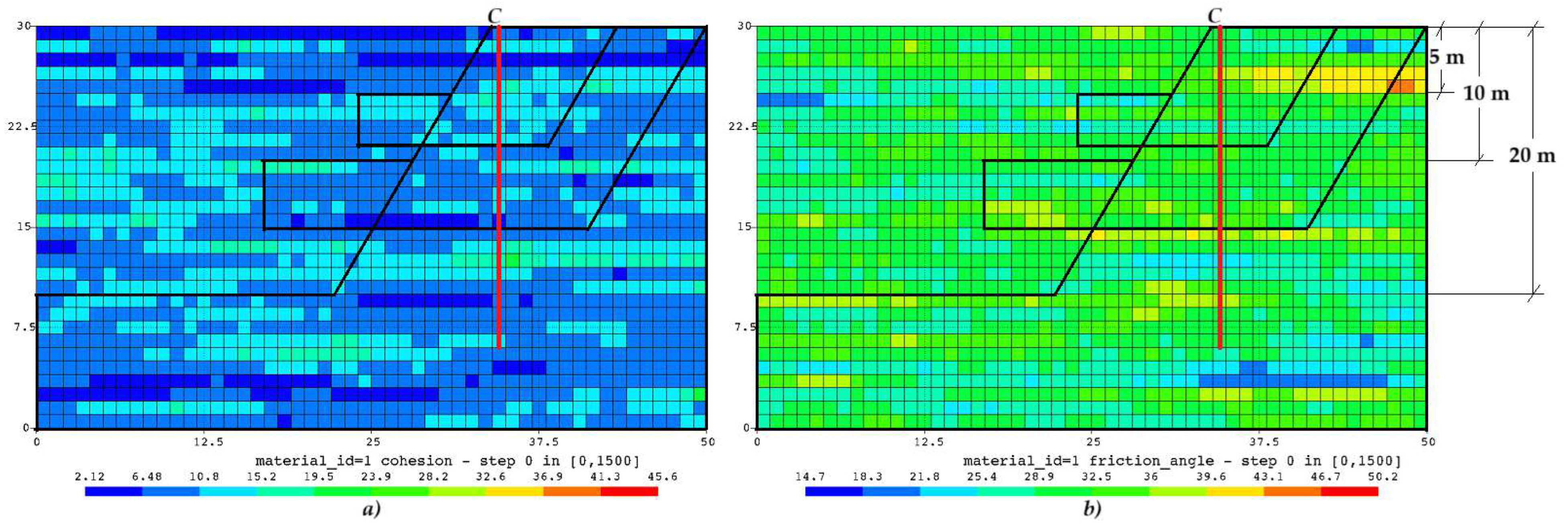
3.2. Generation of the Statistical Meshes

The spatial distribution of c’ and $\varphi$’ in each statistical mesh is generated using the Latin Hypercube Sampling (LHS) technique, as it reduces the complexity and computational effort relatively to a conventional Monte Carlo process [40,41]. LHS preserves the marginal probability distribution of the simulated parameters using fewer samples [42]. This study uses the LHS technique implemented in mechpy using the framework described in Olsson et al. [41].

The description of the spatial variability of $c^{\prime }$ and $\varphi$’ is based on the random fields theory that describes the soil profile using the following parameters used for the generation of the statistical meshes: mean values of the strength parameters, $c_{mg}^{\prime }$ and tan${\varphi }_{mg}^{\prime }$, their coefficient of variation, COV, and their scales of fluctuation, ${\theta }_v$ and ${\theta }_h$ [17,37]. Both properties are assumed to follow the log-normal distribution and are considered uncorrelated. The scale of fluctuation ${\theta }_v$ (as well as ${\theta }_h$) are assumed the same for both strength parameters. The statistical meshes have the spatial distribution of c’ and $\varphi$’, with a different value of these parameters assigned to each element of the meshes, as presented in Figure 3.

The statistical meshes have a width of $50\mathrm{m}$ and a height of $30\mathrm{m}$, discretised into squared statistical elements with the length of the side equal to $1\mathrm{m}$. This size of the squared statistical elements corresponds to the value of the lower scale of fluctuation. As a result of the relation between the dimensions of the statistical meshes and the number of elements therein, the LHS process generates, in the case analysed in this work, 1501 statistical meshes (samples).

3.3. Determination of the Characteristic Values of Strength Parameters

The characteristic values of the strength parameters are estimated for two different scenarios, corresponding to two degrees of knowledge of these parameters.

In the first scenario, a simulation of site characterisation is performed in the statistical meshes of the effective cohesion and of the friction angle. For each sample, the characteristic values of the strength parameters are estimated from the statistical elements intercepted by a vertical line starting at the crest of the slope (point c in Figure 3) down to 1.2 times the depth of the unsupported cut. This process assumes that the characterisation can determine the values of c’ and ${\varphi }^{\prime }$ of the element intercepted by the vertical line, without measurement errors. In this scenario, a set of characteristic strength parameters is obtained from each sample.

In the second scenario, the characteristic values are estimated from the mean and COV used, which are the input parameters used to generate the statistical meshes.

For the first scenario, the chosen location for the vertical line was the one reported as the optimal location to conduct geotechnical exploration for slope stability evaluation [27]. The values of the properties are collected every one meter (the size of the statistical mesh elements adopted in this case), for both c’ and ${\varphi }^{\prime }$ statistic meshes. This leads to a number of values collected for each strength parameter given by $n=1.2h$, with h given in meters. In this first scenario, the characteristic values of c’ and ${\varphi }^{\prime }$ are determined from the abovementioned collected values of the properties using the following expression:

$$X_k=exp\left[Y_m(1-k_n.CO{V}_{lnX})\right]$$

(2)

where $Y_m$ is the mean value of the logarithms of the n strength parameters collected in each sample, $CO{V}_{lnX}$ is the coefficient of variation of those logarithms, $k_n$ is the statistical coefficient related to the type of distribution, the confidence limit, and the number of test values, n.

In the second scenario, Equation (2) is also used, with $Y_m$ and $CO{V}_{lnX}$ being equal to the input values used to generate the samples. These calculations were performed using $n=30$.

In the first scenario, the COV of the soil property is unknown a priori and estimated from the collected values of each soil property; $k_n$ can be obtained from [37]:

$$k_n=t_{n-1}^{0.95}\sqrt{{\displaystyle \frac{\theta }{\mathsf{\ell }}}+{\displaystyle \frac{1}{n}}}$$

(3)

In the second scenario, COV is known a priori, and $k_n$ is determined from

$$k_n=N_{95}\sqrt{{\displaystyle \frac{\theta }{\mathsf{\ell }}}+{\displaystyle \frac{1}{n}}}$$

(4)

In these equations, $t_{n-1}^{0.95}$ is the Student’s t-value for $n-1$ degrees of freedom at a confidence level of 95%; ${\mathit{N}}_{95}$ represents the normal distribution, evaluated for a 95% confidence level with infinite degrees of freedom; $\theta$ is the relevant scale of fluctuation; and ℓ is a measure of the relevant dimension of the problem.

If ${\theta }_v$ is assumed to be small compared to h, the characteristic values can be determined using $\theta /\mathsf{\ell }=0$ in the previous equations. This can be applied in situations where a large volume of ground is involved in the failure mechanism and the characteristic values of the strength parameters can be considered as estimates of their mean values. In other cases, in the present study, $\theta$ is equal to ${\theta }_v$ and ℓ is h.

Moreover, for the first scenario, the characteristic values of the set of soil properties is estimated for each statistical mesh. For the second scenario, a single global set of characteristic values is determined.

3.4. Design

The design values of the soil shear strength parameters are determined from the corresponding characteristic values, using the following equation:

$$X_d={\displaystyle \frac{X_k}{{\gamma }_M}}$$

(5)

where ${\gamma }_M$ is a partial coefficient. In the present paper, ${\gamma }_M$ is set to 1.25 for both $c^{\prime }$ and $tan{\varphi }^{\prime }$. This value is used in the Design Approach 1, combination 2 and in the Design Approach 3 of Eurocode 7 [2]. In some cases, other values of this partial coefficient will be used, and they will be specified later. Only permanent actions are considered in the analyses. Since the partial coefficient for permanent actions is 1.0, ${\gamma }_M$ is the only partial coefficient being applied.

As previously explained, by “design”, in this case, it is meant to determine the maximum unit weight, ${\gamma }_{FELA}$, for which the unsupported cuts verify safety. It is computed using FELA, with homogeneous soil properties equal to $c_d^{\prime }$ and ${\varphi }_d^{\prime }$. The analyses are performed for the initial finite element mesh and for three additional remeshing steps, where the meshes are progressively refined in the zones of higher plastic deformation (Figure 4), according to a methodology based on Martin’s [43] work. The average of both upper- and lower-bound results is calculated, ${\gamma }_{FELA}$.

In the first scenario, 1501 upper- and lower-bound calculations are performed, each one corresponding to each sample, and leading to 1501 values of ${\gamma }_{FELA}$. In the second scenario, a single value is obtained.

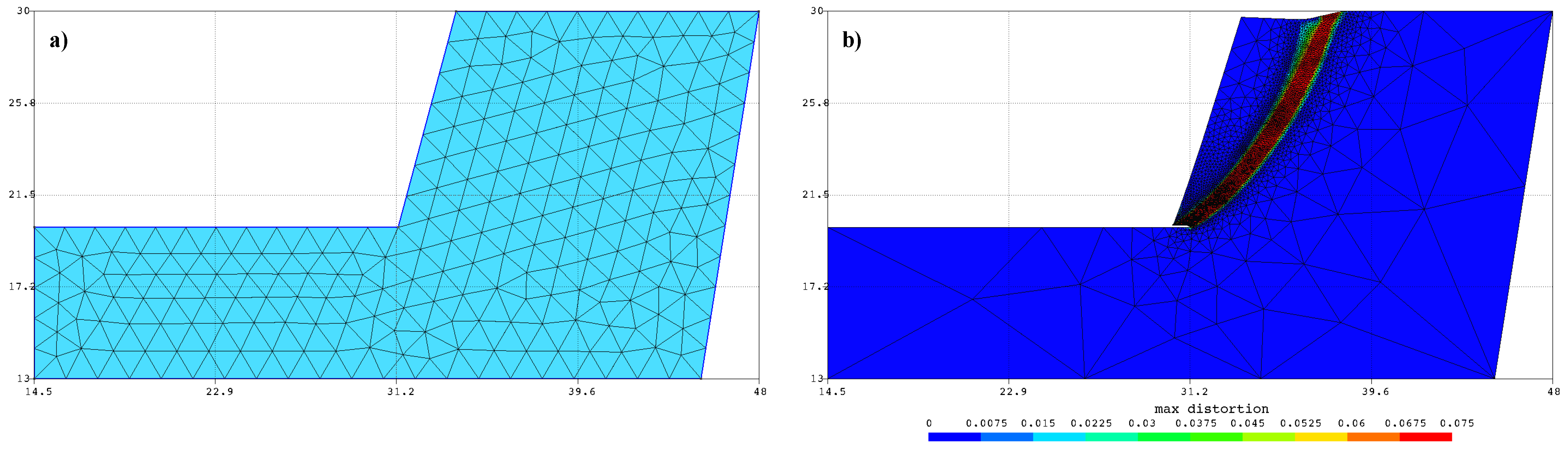
3.5. RFELA Calculations

For a given geometry, a finite element mesh is generated considering quasi-homogeneous finite element sizes. This finite element mesh is superposed to each statistical mesh and, in a mapping process, the soil properties of the element of the statistical mesh at the position of the centroid of each finite element are assigned to this finite element (Figure 3 and Figure 5). This procedure is repeated for each remeshing step. As a consequence, in the last steps, there are zones with very small finite elements and others where the finite elements are quite large. The random field from the statistical mesh does not change, but since the properties are assigned to the centroids of the finite elements during the mapping process, the random field considered in the finite element calculations does change. Nonetheless, this change does not affect the results, as the more refined areas with smaller finite elements are located where the mechanism takes part.

RFELAs are performed for each sample, using mechpy to determine the values of the estimates of the soil unit weight causing collapse for both upper- and lower-bound approaches. For each sample, the analyses are performed using the remeshing process described in the previous section and, for each stage, the mapping procedure described above. The average of both upper- and lower-bound results is calculated for each sample, ${\gamma }_{RFELA}$.

Figure 6 presents the zones of maximum distortion obtained for the same case shown in Figure 5, for the last step of the remeshing process. These results, as well as the areas where the finite element mesh was more refined, allow us to infer the mechanism that is developed.

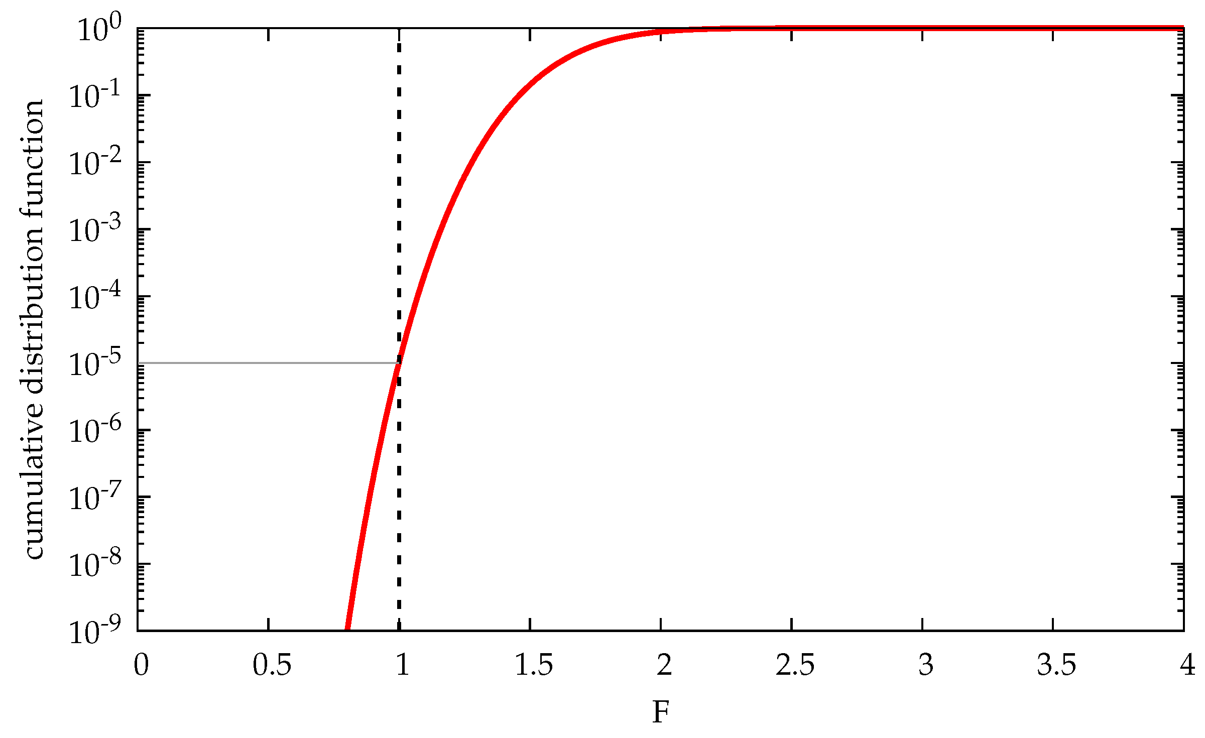
3.6. Probability of Failure and Reliability Analysis

The probability of failure is estimated using direct reliability analysis of a performance function F, given by

$$F={\displaystyle \frac{{\gamma }_{RFELA}}{{\gamma }_{FELA}(1+CO{V}_{\gamma }\Delta )}}$$

(6)

where $\Delta$ accounts for the uncertainty in the actions and consists of a random number that follows the standard normal distribution (with mean 0 and standard deviation 1). $CO{V}_{\gamma }$ is assumed to be $0.1$, which is a common value of the coefficient of variation of the soil unit weight [11,14]. The probability of $F\le 1$ is estimated using the cumulative Log-normal distribution function.

Figure 7 shows the cumulative distribution function of F for an example with $h=10\mathrm{m}$, $\beta ={75}^{\circ }$, ${\varphi }_{mg}^{\prime }={30}^{\circ }$, $c_{mg}^{\prime }=10\mathrm{kPa}$, $\Delta \ne 0$, the 1st scenario, and assuming $\theta /\mathsf{\ell }=0$ in Equation (3). From this figure, it can be seen that, for this case, the probability of failure, corresponding to $F=1$, is around ${10}^{-5}$.

4. Cases Analysed

We aimed to study the influence on the probability of failure of the following parameters using the cases analysed:

• The value of the effective cohesion, $c_{mg}^{\prime }$;
• The dimensionless scale of fluctuation, ${\Theta }_v={\theta }_v/h$;
• The geometry of the cut (h and $\beta$) and of the soil friction angle, ${\varphi }_{mg}^{\prime }$.

4.1. Influence of the Value of the Effective Cohesion

Calculations were performed for ${\varphi }_{mg}^{\prime }={30}^{\circ }$, $\beta ={75}^{\circ }$, and for two values of h—5 and $10\mathrm{m}$. For $h=5\mathrm{m}$, calculations were performed for four values of $c_{mg}^{\prime }$—1, $2.5$, 10, and $100\mathrm{kPa}$; for $h=10\mathrm{m}$, two values of $c_{mg}^{\prime }$ were used, 5 and 10 kPa. The coefficient of variation used for $c^{\prime }$ and for $tan{\varphi }^{\prime }$ was $0.15$ and $0.30$, respectively, and the vertical and horizontal scales of fluctuation were 1 and $30\mathrm{m}$. These values for the coefficient of variation and for the scales of fluctuation are typical of sedimentary soils [11,14,44,45].

The post-processing of the computation outcomes was conducted according to the procedures detailed in Section 3, and the results obtained for the probability of failure are shown in

Table 1. Results of the probability of failure for different values of $c_{mg}^{\prime }$ considering $\theta /\mathsf{\ell }=0$ in Equation (3).

h	${\mathit{\varphi }}_{\mathit{mg}}^{\prime }{(}^{\circ })$/COV	${\mathit{c}}_{\mathit{mg}}^{\prime }\left(\mathbf{kPa}\right)$/COV	${\mathit{\theta }}_{\mathit{v}}/\mathit{h}$	$\mathit{\beta }$	1st Scenario		2nd Scenario
(m)				${(}^{\circ })$	$\Delta =\mathbf{0}$	$\Delta \ne \mathbf{0}$	$\Delta =\mathbf{0}$	$\Delta \ne \mathbf{0}$
5	30/0.15	1/0.3	0.20	75	4 $\times {10}^{-9}$	5 $\times {10}^{-6}$	8 $\times {10}^{-4}$	4 $\times {10}^{-3}$
		2.5/0.3			3 $\times {10}^{-9}$	8 $\times {10}^{-6}$	1 $\times {10}^{-3}$	5 $\times {10}^{-3}$
		10/0.3			1 $\times {10}^{-9}$	8 $\times {10}^{-6}$	1 $\times {10}^{-3}$	5 $\times {10}^{-3}$
		100/0.3			1 $\times {10}^{-9}$	5 $\times {10}^{-6}$	9 $\times {10}^{-4}$	4 $\times {10}^{-3}$
10	30/0.15	5/0.3	0.1	75	3 $\times {10}^{-13}$	8 $\times {10}^{-6}$	1 $\times {10}^{-5}$	7 $\times {10}^{-4}$
		10/0.3			2 $\times {10}^{-13}$	1 $\times {10}^{-5}$	9 $\times {10}^{-6}$	7 $\times {10}^{-4}$

. The analysis of the probabilities of failure obtained is included in the results presented in Section 4.3; in this section, the most relevant issue is the fact the probabilities of failure obtained are practically independent of the values of $c_{mg}^{\prime }$ (when the design value of the actions is equal to the design value of the resistance, which is the process adopted in Section 3.4). This allows us to proceed with the study considering a single value of $c_{mg}^{\prime }$.

4.2. Influence of the Dimensionless Scale of Fluctuation

To assess the influence of the dimensionless scale of fluctuation, calculations were performed considering ${\varphi }_{mg}^{\prime }={30}^{\circ }$, $c_{mg}^{\prime }=10\mathrm{kPa}$, $\beta ={75}^{\circ }$, and three values of h—5, 10, and $20\mathrm{m}$—and different ${\theta }_v$ values were chosen to obtain, for each value of h, four different values of ${\Theta }_v={\theta }_v/h$ (

Table 2. Results of the probability of failure for different values of h and ${\Theta }_v$, obtained for ${\varphi }_{mg}^{\prime }={30}^{\circ }$, ${\mathit{c}}_{mg}^{\prime }=10\mathrm{kPa}$, $COV=0.1$ and $0.3$, and $\beta ={75}^{\circ }$.

h	${\mathit{\theta }}_{\mathit{v}}$	${\mathbf{\Theta }}_{\mathit{v}}$	$\mathit{\theta }/\mathit{\ell }=0$				$\mathit{\theta }/\mathit{\ell }\ne 0$
			1st Scenario		2nd Scenario		1st Scenario		2nd Scenario
(m)	(m)		$\Delta =\mathbf{0}$	$\Delta \ne \mathbf{0}$	$\Delta =\mathbf{0}$	$\Delta \ne \mathbf{0}$	$\Delta =\mathbf{0}$	$\Delta \ne \mathbf{0}$	$\Delta =\mathbf{0}$	$\Delta \ne \mathbf{0}$
5	0.25	0.05	2 $\times {10}^{-15}$	3 $\times {10}^{-5}$	4 $\times {10}^{-9}$	1 $\times {10}^{-4}$	6 $\times {10}^{-18}$	4 $\times {10}^{-6}$	3 $\times {10}^{-11}$	2 $\times {10}^{-5}$
	0.50	0.10	1 $\times {10}^{-13}$	1 $\times {10}^{-5}$	1 $\times {10}^{-5}$	8 $\times {10}^{-4}$	4 $\times {10}^{-15}$	8 $\times {10}^{-7}$	1 $\times {10}^{-7}$	6 $\times {10}^{-5}$
	0.75	0.15	9 $\times {10}^{-12}$	6 $\times {10}^{-6}$	2 $\times {10}^{-4}$	2 $\times {10}^{-3}$	7 $\times {10}^{-12}$	8 $\times {10}^{-7}$	2 $\times {10}^{-6}$	1 $\times {10}^{-4}$
	1.00	0.20	1 $\times {10}^{-9}$	8 $\times {10}^{-6}$	1 $\times {10}^{-3}$	5 $\times {10}^{-3}$	2 $\times {10}^{-9}$	2 $\times {10}^{-6}$	2 $\times {10}^{-5}$	2 $\times {10}^{-4}$
10	0.50	0.05	3 $\times {10}^{-16}$	3 $\times {10}^{-5}$	3 $\times {10}^{-9}$	1 $\times {10}^{-4}$	5 $\times {10}^{-19}$	3 $\times {10}^{-6}$	2 $\times {10}^{-11}$	1 $\times {10}^{-5}$
	1.00	0.10	2 $\times {10}^{-13}$	1 $\times {10}^{-5}$	9 $\times {10}^{-6}$	7 $\times {10}^{-4}$	9 $\times {10}^{-15}$	8 $\times {10}^{-7}$	8 $\times {10}^{-8}$	5 $\times {10}^{-5}$
	1.50	0.15	6 $\times {10}^{-12}$	5 $\times {10}^{-6}$	2 $\times {10}^{-4}$	2 $\times {10}^{-3}$	3 $\times {10}^{-12}$	5 $\times {10}^{-7}$	2 $\times {10}^{-6}$	9 $\times {10}^{-5}$
	2.00	0.20	2 $\times {10}^{-10}$	5 $\times {10}^{-6}$	9 $\times {10}^{-4}$	4 $\times {10}^{-3}$	6 $\times {10}^{-10}$	1 $\times {10}^{-6}$	9 $\times {10}^{-6}$	2 $\times {10}^{-4}$
20	1.00	0.05	6 $\times {10}^{-16}$	3 $\times {10}^{-5}$	2 $\times {10}^{-9}$	1 $\times {10}^{-4}$	3 $\times {10}^{-18}$	3 $\times {10}^{-6}$	1 $\times {10}^{-11}$	1 $\times {10}^{-5}$
	2.00	0.10	5 $\times {10}^{-14}$	7 $\times {10}^{-6}$	1 $\times {10}^{-5}$	7 $\times {10}^{-4}$	2 $\times {10}^{-15}$	5 $\times {10}^{-7}$	1 $\times {10}^{-7}$	5 $\times {10}^{-5}$
	3.00	0.15	2 $\times {10}^{-12}$	4 $\times {10}^{-6}$	2 $\times {10}^{-4}$	2 $\times {10}^{-3}$	1 $\times {10}^{-12}$	5 $\times {10}^{-7}$	2 $\times {10}^{-6}$	1 $\times {10}^{-4}$
	4.00	0.20	4 $\times {10}^{-10}$	5 $\times {10}^{-6}$	9 $\times {10}^{-4}$	4 $\times {10}^{-3}$	1 $\times {10}^{-9}$	1 $\times {10}^{-6}$	1 $\times {10}^{-5}$	2 $\times {10}^{-4}$

). The horizontal scale of fluctuation was considered equal to 30 times the vertical scale. The coefficient of variation used for $c^{\prime }$ and for $tan{\varphi }^{\prime }$ were the same as those used in the previous section.

The results obtained for the probability of failure are included in Table 2, and represented in Figure 8. The results show that the probabilities of failure are very close for different values of ${\theta }_v$ and h, if ${\Theta }_v$ is the same. These results allowed us to proceed with the study considering different values of h and a single value of ${\theta }_v$, and therefore, different values of the relevant parameter, ${\Theta }_v$.

It can also be seen that for the second scenario, the probability of failure increases with ${\Theta }_v$, whereas for the first scenario, there is not a clear tendency and it overall varies in a smaller range.

4.3. Influence of the Geometry of the Cut and of the Soil Friction Angle

The study considers nine unsupported cut geometries resulting from combining three different depths, $h=5$, 10, and $20\mathrm{m}$, with three inclinations, $\beta ={45}^{\circ }$, ${60}^{\circ }$, and ${75}^{\circ }$, having the slope crest, C, in common (Figure 3).

All geometries were combined with soils with ${\varphi }_{mg}^{\prime }={30}^{\circ }$, ${35}^{\circ }$, and ${40}^{\circ }$, with a COV of $0.15$, and $c_{mg}^{\prime }=10\mathrm{kPa}$, with a COV of $0.30$. Both parameters have vertical and horizontal scales of fluctuation, ${\theta }_v$ and ${\theta }_h$ of $1\mathrm{m}$ and $30\mathrm{m}$, respectively. These values are within the limits reported in the literature [11,12,14,44,45].

Table 3. Results of the probability of failure obtained considering $\theta /\mathsf{\ell }=0$ in Equations (3) and (4).

$\mathit{h}\left(\mathbf{m}\right)$	${\mathit{\varphi }}_{\mathit{mg}}^{\prime }{(}^{\circ })/\mathit{COV}$	${\mathit{c}}_{\mathit{mg}}^{\prime }\left(\mathbf{kPa}\right)/\mathit{COV}$	${\mathit{\theta }}_{\mathit{v}}/\mathit{h}$	$\mathit{\beta }{(}^{\circ })$	1st Scenario		2nd Scenario
					$\Delta =\mathbf{0}$	$\Delta \ne \mathbf{0}$	$\Delta =\mathbf{0}$	$\Delta \ne \mathbf{0}$
5	30/0.15	10/0.30	0.2	45	1 $\times {10}^{-7}$	3 $\times {10}^{-6}$	2 $\times {10}^{-3}$	3 $\times {10}^{-3}$
				60	2 $\times {10}^{-9}$	3 $\times {10}^{-6}$	1 $\times {10}^{-3}$	3 $\times {10}^{-3}$
				75	1 $\times {10}^{-9}$	8 $\times {10}^{-6}$	1 $\times {10}^{-3}$	5 $\times {10}^{-3}$
	35/0.15			45	—	—	—	—
				60	2 $\times {10}^{-9}$	1 $\times {10}^{-6}$	8 $\times {10}^{-4}$	3 $\times {10}^{-3}$
				75	6 $\times {10}^{-10}$	4 $\times {10}^{-6}$	8 $\times {10}^{-4}$	4 $\times {10}^{-3}$
	40/0.15			45	—	—	—	—
				60	3 $\times {10}^{-9}$	5 $\times {10}^{-7}$	9 $\times {10}^{-4}$	2 $\times {10}^{-3}$
				75	1 $\times {10}^{-10}$	1 $\times {10}^{-6}$	7 $\times {10}^{-4}$	3 $\times {10}^{-3}$
10	30/0.15	10/0.30	0.1	45	1 $\times {10}^{-9}$	7 $\times {10}^{-7}$	8 $\times {10}^{-6}$	1 $\times {10}^{-4}$
				60	3 $\times {10}^{-12}$	2 $\times {10}^{-6}$	5 $\times {10}^{-6}$	3 $\times {10}^{-4}$
				75	2 $\times {10}^{-13}$	1 $\times {10}^{-5}$	9 $\times {10}^{-6}$	7 $\times {10}^{-4}$
	35/0.15			45	—	—	—	—
				60	6 $\times {10}^{-12}$	8 $\times {10}^{-7}$	5 $\times {10}^{-6}$	2 $\times {10}^{-4}$
				75	4 $\times {10}^{-14}$	3 $\times {10}^{-6}$	6 $\times {10}^{-6}$	5 $\times {10}^{-4}$
	40/0.15			45	—	—	—	—
				60	5 $\times {10}^{-12}$	2 $\times {10}^{-7}$	6 $\times {10}^{-6}$	1 $\times {10}^{-4}$
				75	1 $\times {10}^{-14}$	1 $\times {10}^{-6}$	5 $\times {10}^{-6}$	3 $\times {10}^{-4}$
20	30/0.15	10/0.30	0.05	45	2 $\times {10}^{-11}$	5 $\times {10}^{-7}$	4 $\times {10}^{-9}$	7 $\times {10}^{-7}$
				60	3 $\times {10}^{-14}$	5 $\times {10}^{-6}$	2 $\times {10}^{-9}$	3 $\times {10}^{-5}$
				75	6 $\times {10}^{-16}$	3 $\times {10}^{-5}$	2 $\times {10}^{-9}$	1 $\times {10}^{-4}$
	35/0.15			45	2 $\times {10}^{-10}$	8 $\times {10}^{-8}$	3 $\times {10}^{-8}$	1 $\times {10}^{-6}$
				60	9 $\times {10}^{-15}$	9 $\times {10}^{-7}$	6 $\times {10}^{-10}$	9 $\times {10}^{-6}$
				75	3 $\times {10}^{-17}$	8 $\times {10}^{-6}$	6 $\times {10}^{-10}$	5 $\times {10}^{-5}$
	40/0.15			45	—	—	—	—
				60	3 $\times {10}^{-16}$	7 $\times {10}^{-8}$	7 $\times {10}^{-10}$	3 $\times {10}^{-6}$
				75	2 $\times {10}^{-19}$	2 $\times {10}^{-6}$	5 $\times {10}^{-10}$	2 $\times {10}^{-5}$

summarises the results of the probability of failure assuming $\theta /\mathsf{\ell }=0$ in Equations (3) and (4);

Table 4. Results of the probability of failure obtained considering $\theta /\mathsf{\ell }={\Theta }_v$ in Equations (3) and (4).

$\mathit{h}\left(\mathbf{m}\right)$	${\mathit{\varphi }}_{\mathit{mg}}^{\prime }{(}^{\circ })/\mathit{COV}$	${\mathit{c}}_{\mathit{mg}}^{\prime }\left(\mathbf{kPa}\right)/\mathit{COV}$	${\mathit{\theta }}_{\mathit{v}}/\mathit{h}$	$\mathit{\beta }{(}^{\circ })$	1st Scenario		2nd Scenario
					$\Delta =\mathbf{0}$	$\Delta \ne \mathbf{0}$	$\Delta =\mathbf{0}$	$\Delta \ne \mathbf{0}$
5	30/0.15	10/0.30	0.2	45	2 $\times {10}^{-8}$	3 $\times {10}^{-7}$	5 $\times {10}^{-5}$	1 $\times {10}^{-4}$
				60	1 $\times {10}^{-9}$	5 $\times {10}^{-7}$	1 $\times {10}^{-5}$	1 $\times {10}^{-4}$
				75	2 $\times {10}^{-9}$	2 $\times {10}^{-6}$	2 $\times {10}^{-5}$	2 $\times {10}^{-4}$
	35/0.15			45	—	—	—	—
				60	1 $\times {10}^{-9}$	2 $\times {10}^{-7}$	1 $\times {10}^{-5}$	8 $\times {10}^{-5}$
				75	1 $\times {10}^{-9}$	8 $\times {10}^{-7}$	1 $\times {10}^{-5}$	1 $\times {10}^{-4}$
	40/0.15			45	—	—	—	—
				60	8 $\times {10}^{-10}$	8 $\times {10}^{-8}$	2 $\times {10}^{-5}$	9 $\times {10}^{-5}$
				75	3 $\times {10}^{-10}$	3 $\times {10}^{-7}$	9 $\times {10}^{-6}$	1 $\times {10}^{-4}$
10	30/0.15	10/0.30	0.1	45	3 $\times {10}^{-11}$	3 $\times {10}^{-8}$	1 $\times {10}^{-7}$	4 $\times {10}^{-6}$
				60	4 $\times {10}^{-14}$	1 $\times {10}^{-7}$	3 $\times {10}^{-8}$	1 $\times {10}^{-5}$
				75	9 $\times {10}^{-15}$	8 $\times {10}^{-7}$	8 $\times {10}^{-8}$	4 $\times {10}^{-5}$
	35/0.15			45	—	—	—	—
				60	1 $\times {10}^{-13}$	4 $\times {10}^{-8}$	5 $\times {10}^{-8}$	7 $\times {10}^{-6}$
				75	2 $\times {10}^{-15}$	2 $\times {10}^{-7}$	5 $\times {10}^{-8}$	3 $\times {10}^{-5}$
	40/0.15			45	—	—	—	—
				60	9 $\times {10}^{-14}$	8 $\times {10}^{-9}$	9 $\times {10}^{-8}$	5 $\times {10}^{-6}$
				75	4 $\times {10}^{-16}$	6 $\times {10}^{-8}$	4 $\times {10}^{-8}$	2 $\times {10}^{-5}$
20	30/0.15	10/0.30	0.05	45	2 $\times {10}^{-13}$	3 $\times {10}^{-8}$	6 $\times {10}^{-11}$	2 $\times {10}^{-7}$
				60	1 $\times {10}^{-16}$	4 $\times {10}^{-7}$	1 $\times {10}^{-11}$	3 $\times {10}^{-6}$
				75	3 $\times {10}^{-18}$	3 $\times {10}^{-6}$	1 $\times {10}^{-11}$	1 $\times {10}^{-5}$
	35/0.15			45	3 $\times {10}^{-12}$	5 $\times {10}^{-9}$	9 $\times {10}^{-10}$	1 $\times {10}^{-7}$
				60	2 $\times {10}^{-17}$	6 $\times {10}^{-8}$	5 $\times {10}^{-12}$	6 $\times {10}^{-7}$
				75	7 $\times {10}^{-20}$	9 $\times {10}^{-7}$	4 $\times {10}^{-12}$	5 $\times {10}^{-6}$
	40/0.15			45	—	—	—	—
				60	6 $\times {10}^{-19}$	3 $\times {10}^{-9}$	8 $\times {10}^{-12}$	2 $\times {10}^{-7}$
				75	3 $\times {10}^{-22}$	1 $\times {10}^{-7}$	3 $\times {10}^{-12}$	2 $\times {10}^{-6}$

shows the ones for $\theta /\mathsf{\ell }={\Theta }_v$ in the same equations. These results are also shown in Figure 9.

Table 3 and Table 4 and the graphics in Figure 9 do not always show the results obtained for $\beta ={45}^{\circ }$. In fact, for this case, and for some situations where the soil friction angle is 35 and ${40}^{\circ }$, the values obtained for the performance function Equation (6) cannot be appropriately described by the Log-normal distribution (and, also, no other distribution could be found to be able to describe them).

From Figure 9, it can be concluded that the probabilities of failure obtained for the second scenario are higher than the ones for the first scenario. This is an interesting result, although expected, and emphasises the importance of soil characterisation performed at the exact location of each project. Also, more inclined slopes (greater values of $\beta$) have greater probability of failure, and for the second scenario, the probability of failure decreases as the excavation depth, h, increases. This tendency is more accentuated when $\theta /\mathsf{\ell }$ is assumed equal to zero in Equation (4). It seems, therefore, that a single characteristic value determined from the global soil properties (in this case, from the friction angle used to generate the samples) can better describe the soil when the excavation depth is high, and therefore, the probability of failure obtained for the first and the second scenarios are closer. In fact, the probabilities of failure obtained for the first scenario seem more constant (and without a clear tendency) than the one obtained for the second scenario.

As expected, the probability of failure obtained when $\theta /\mathsf{\ell }={\Theta }_v$ is lower than the one obtained when $\theta /\mathsf{\ell }$ is assumed zero, as the first case always results in lower characteristic values. It can also be seen that for the second scenario, and particularly for the case when $\theta /\mathsf{\ell }$ is assumed zero, the probability of failure can be higher than ${10}^{-4}$.

It seems, therefore, that the partial coefficient of $1.25$ is sufficient to allow for the probabilities of failure lower than ${10}^{-4}$ when the soil is carefully characterised (first scenario).

And even for the cases where the soil is not carefully characterised but the soil is very well known (2nd scenario), the same partial coefficient would ensure the minimum probability of failure in most cases if $\theta /\mathsf{\ell }={\Theta }_v$ is correctly considered in Equation (4); a slight increase in the partial coefficient to 1.3 would be sufficient to cover all the analysed cases. If, however, $\theta /\mathsf{\ell }$ is considered zero in that equation, a greater partial coefficient is needed.

Such an analysis was performed for the case ${\varphi }_{mg}^{\prime }={30}^{\circ }$ and $h=5\mathrm{m}$, which gave the highest probabilities of failure for the second scenario and $\theta /\mathsf{\ell }=0$ (see Figure 9). The results are presented in Figure 10, which also shows the results for $\theta /\mathsf{\ell }={\Theta }_v$, for comparison. It can be seen that for $\theta /\mathsf{\ell }=0$, a partial coefficient of 1.5 (in fact, between 1.4 and 1.5) is needed, in order to obtain a probability of failure of less than ${10}^{-4}$.

The minimum values of the safety factors of 1.25 and 1.4–1.5 should therefore be applied, depending on the type of soil characterization, in the design of unsupported excavation slopes.

For other types of geotechnical structures, the same procedure used in this paper can be used to assess the methods for determining the characteristic values of the soil parameters and of the values of the safety factors.

5. Conclusions

It was shown how a sustainable design of unsupported cuts involves a careful process of determining the characteristic values of the soil strength parameters and the usage of appropriate safety factors in order to obtain an adequate probability of failure.

For simple geometries of unsupported cuts and different soil strength parameters, a procedure involving the generation of samples of the soil mass, considering the spacial distribution of those parameters, was carried out. It was applied to determine the probability of failure of the unsupported cuts considering two scenarios, corresponding to two degrees of knowledge of the soil strength parameters. In the first scenario, soil characterisation is simulated in the generated soil samples and the characteristic values of the strength parameters are obtained for each sample. In the second scenario, the characteristic values are determined from the parameters used to generate the samples.

This analysis allowed us to conclude the following:

• The value of $c^{\prime }$ does not significantly influence the probability of failure for cuts where the design value of the actions equal the design value of the resistances;
• The probability of failure depends on the dimensionless scale of fluctuation, and not on the scale of fluctuation or excavation depth, which is considered isolated;
• Combining careful soil characterisation performed at the exact location of the cut with a partial coefficient of 1.25 applied to the strength parameters ensures a probability of failure less than ${10}^{-4}$;
• For the cases where the soil is not carefully characterised but the soil is very well known, a slightly larger value of the partial coefficient is needed to ensure the same probability of failure if the scale of fluctuation is considered correctly when determining the characteristic values of the strength parameters; if the scale of fluctuation is not considered, a partial factor of 1.4–1.5 is needed.

These minimum safety factors are, therefore, recommended to designers involved in unsupported excavation slopes.

The procedure used in this paper can be applied to other types of geotechnical structures, such as shallow foundations, retaining walls, tunnels, etc., allowing in each case the evaluation of the methods to determine the characteristic values of the soil parameters and of the values of the safety factors adopted.

References

1. Basu, D.; Puppala, A.; Misra, A.; Chittoori, B. Sustainability in Geotechnical Engineering. In Proceedings of the 18th International Conference on Soil Mechanics and Geotechnical, Paris, France, 2–6 September 2013; pp. 3155–3162. Available online: https://www.cfms-sols.org/sites/default/files/Actes/3171-3174.pdf (accessed on 1 September 2024).
2. EN1997-1. Eurocode 7: Geotechnical Design—Part 1: General Rules; CEN, European Committee for Standardization: Brussels, Belgium, 2004.
3. Lumb, P. Safety factors and the probability distribution of soil strength. Can. Geotech. J. 1970, 7, 225–242. [Google Scholar] [CrossRef]
4. Meyerhof, G.G. Safety factors in soil mechanics. Can. Geotech. J. 1970, 7, 349–355. [Google Scholar] [CrossRef]
5. Meyerhof, G. Limit states design in geotechnical engineering. Struct. Saf. 1982, 1, 67–71. [Google Scholar] [CrossRef]
6. Santamarina, J.C.; Altschaeffl, A.G.; Chameau, J.L. Reliability of Slopes: Incorporating Qualitative Information. National Research Council (U.S.), Transportation Research Board, Report TRR 1343. 1992, pp. 1–5. Available online: http://onlinepubs.trb.org/Onlinepubs/trr/1992/1343/1343-001.pdf (accessed on 1 September 2024).
7. Baecher, G.B.; Christian, J.T. Reliability and Statistics in Geotechnical Engineering; John Wiley & Sons: Hoboken, NJ, USA, 2003. [Google Scholar]
8. Orr, T.L. Selection of characteristic values and partial factors in geotechnical designs to Eurocode 7. Comput. Geotech. 2000, 26, 263–279. [Google Scholar] [CrossRef]
9. Ching, J.; Phoon, K.K.; Chen, K.F.; Orr, T.L.; Schneider, H.R. Statistical determination of multivariate characteristic values for Eurocode 7. Struct. Saf. 2020, 82, 101893. [Google Scholar] [CrossRef]
10. Länsivaara, T.; Phoon, K.K.; Ching, J. What is a characteristic value for soils? Georisk Assess. Manag. Risk Eng. Syst. Geohazards 2022, 16, 199–224. [Google Scholar] [CrossRef]
11. Phoon, K.K.; Kulhawy, F.H. Characterization of geotechnical variability. Can. Geotech. J. 1999, 36, 612–624. [Google Scholar] [CrossRef]
12. Cao, Z.; Wang, Y.; Li, D. Probabilistic Approaches for Geotechnical Site Characterization and Slope Stability Analysis; Springer: Berlin/Heidelberg, Germany, 2017. [Google Scholar] [CrossRef]
13. Kulhawy, F.; Prakoso, W.; Phoon, K. Uncertainty in basic laboratory and field properties of geomaterials. In Geotechnical Engineering Education and Training; CRC Press: London, UK, 2020; pp. 297–302. [Google Scholar] [CrossRef]
14. Phoon, K.K.; Shuku, T.; Ching, J. Uncertainty, Modeling, and Decision Making in Geotechnics; CRC Press: Boca Raton, FL, USA, 2023. [Google Scholar] [CrossRef]
15. Vanmarcke, E.H. Reliability of Earth Slopes. J. Geotech. Eng. Div. 1977, 103, 1247–1265. [Google Scholar] [CrossRef]
16. Mostyn, G.R.; Soo, S. The effect of auto-correlation on the probability of failure of slopes. In Proceedings of the Effect of Auto-Correlation on the Probability of Failure of Slopes, Christchurch, New Zealand, 3–7 February 1992; pp. 542–546. Available online: https://www.issmge.org/uploads/publications/89/99/6ANZ_095.pdf (accessed on 1 September 2024).
17. Griffiths, D.V.; Fenton, G.A. Probabilistic Slope Stability Analysis by Finite Elements. J. Geotech. Geoenviron. Eng. 2004, 130, 507–518. [Google Scholar] [CrossRef]
18. Cho, S.E. Effects of spatial variability of soil properties on slope stability. Eng. Geol. 2007, 92, 97–109. [Google Scholar] [CrossRef]
19. Suchomel, R.; Mašín, D. Comparison of different probabilistic methods for predicting stability of a slope in spatially variable cϕ soil. Comput. Geotech. 2010, 37, 132–140. [Google Scholar] [CrossRef]
20. Chok, Y.H.; Jaksa, M.B.; Griffiths, D.V.; Fenton, G.A.; Kaggwa, W.S. Probabilistic analysis of a spatially variable cϕ slope. Aust. Geomech. J. 2015, 50, 17–27. [Google Scholar]
21. Agbaje, S.; Zhang, X.; Ward, D.; Dhimitri, L.; Patelli, E. Spatial variability characteristics of the effective friction angle of Crag deposits and its effects on slope stability. Comput. Geotech. 2022, 141, 104532. [Google Scholar] [CrossRef]
22. Chuaiwate, P.; Jaritngam, S.; Panedpojaman, P.; Konkong, N. Probabilistic Analysis of Slope against Uncertain Soil Parameters. Sustainability 2022, 14, 14530. [Google Scholar] [CrossRef]
23. Peng, P.; Li, Z.; Zhang, X.; Liu, W.; Sui, S.; Xu, H. Slope Failure Risk Assessment Considering Both the Randomness of Groundwater Level and Soil Shear Strength Parameters. Sustainability 2023, 15, 7464. [Google Scholar] [CrossRef]
24. Yang, R.; Huang, J.; Griffiths, D.V.; Meng, J.; Fenton, G.A. Optimal geotechnical site investigations for slope design. Comput. Geotech. 2019, 114, 103111. [Google Scholar] [CrossRef]
25. Yang, R.; Huang, J.; Griffiths, D.V.; Li, J.; Sheng, D. Importance of soil property sampling location in slope stability assessment. Can. Geotech. J. 2019, 56, 335–346. [Google Scholar] [CrossRef]
26. Jiang, S.H.; Papaioannou, I.; Straub, D. Optimization of Site-Exploration Programs for Slope-Reliability Assessment. Asce-Asme J. Risk Uncertain. Eng. Syst. Part Civ. Eng. 2020, 6, 04020004. [Google Scholar] [CrossRef]
27. Yang, R.; Huang, J.; Griffiths, D.V. Optimal geotechnical site investigations for slope reliability assessment considering measurement errors. Eng. Geol. 2022, 297, 106497. [Google Scholar] [CrossRef]
28. de Koker, N.; Day, P.; Zwiers, A. Assessment of reliability-based design of stable slopes. Can. Geotech. J. 2019, 56, 495–504. [Google Scholar] [CrossRef]
29. Knuuti, M.; Länsivaara, T. Performance of Variable Partial Factor approach in a slope design. In Proceedings of the 13th International Conference on Applications of Statistics and Probability in Civil Engineering(ICASP13), Seoul, Republic of Korea, 26–30 May 2019. [Google Scholar] [CrossRef]
30. Länsivaara, T.; Poutanen, T. Slope stability with partial safety factor method. In Proceedings of the 18th International Conference on Soil Mechanics and Geotechnical Engineering, Paris, France, 2–6 September 2013; Available online: https://www.cfms-sols.org/sites/default/files/Actes/1823-1826.pdf (accessed on 1 September 2024).
31. Kavvadas, M.; Karlaftis, M.; Fortsakis, P.; Stylianidi, E. Probabilistic analysis in slope stability. In Proceedings of the 17th International Conference on Soil Mechanics and Geotechnical Engineering: The Academia and Practice of Geotechnical Engineering, Alexandria, Egypt, 5–9 October 2009; Volume 2, pp. 1650–1653. [Google Scholar] [CrossRef]
32. Vicente da Silva, M.; Antão, A.N. Software Mechpy. 2013. Available online: http://geocluster.dec.fct.unl.pt/mechpy/ (accessed on 2 February 2023).
33. Simões, J.T.; Neves, L.C.; Antão, A.N.; Guerra, N.M.C. Probabilistic analysis of bearing capacity of shallow foundations using three-dimensional limit analyses. Int. J. Comput. Methods 2014, 11, 1342008. [Google Scholar] [CrossRef]
34. Rantanen, T. Influence of the Variability of Soil Properties on the Stability of Shallow Tunnels in Soils Under Undrained Eonditions. Master’s Thesis, Faculdade de Ciências e Tecnologia, Universidade Nova de Lisboa, Lisbon, Portugal, 2016. (In Portuguese). [Google Scholar]
35. Andrade Viana, L.; Antão, A.; Vicente da Silva, M.; Guerra, N. The application of limit analysis to the study of basal failure of deep excavations in clay considering the spatial distribution of soil strength. In Proceedings of the XVII European Conference on Soil Mechanics and Geotechnical Engineening, Icelandic Geotechnical Society, Reykjavík, Iceland, 1–6 September 2019. Available online: https://www.ecsmge-2019.com/uploads/2/1/7/9/21790806/0909-ecsmge-2019_viana-v2.pdf (accessed on 1 September 2024).
36. Simões, J.; Neves, L.C.; Antão, A.N.; Guerra, N.M. Reliability assessment of shallow foundations on undrained soils considering soil spatial variability. Comput. Geotech. 2020, 119, 103369. [Google Scholar] [CrossRef]
37. Vanmarcke, E.H. Probabilistic Modeling of Soil Profiles. J. Geotech. Eng. Div. 1977, 103, 1227–1246. [Google Scholar] [CrossRef]
38. Fenton, G.A.; Griffiths, D.V. Risk Assessment in Geotechnical Engineering; John Wiley & Sons: Hoboken, NJ, USA, 2008; p. 461. [Google Scholar]
39. Vicente da Silva, M.; Deusdado, N.; Antão, A.N. Lower and upper bound limit analysis via the alternating direction method of multipliers. Comput. Geotech. 2020, 124, 103571. [Google Scholar] [CrossRef]
40. McKay, M.D.; Beckman, R.J.; Conover, W.J. Comparison of three methods for selecting values of input variables in the analysis of output from a computer code. Technometrics 1979, 21, 239–245. [Google Scholar] [CrossRef]
41. Olsson, A.; Sandberg, G.; Dahlblom, O. On Latin hypercube sampling for structural reliability analysis. Struct. Saf. 2003, 25, 47–68. [Google Scholar] [CrossRef]
42. Huntington, D.E.; Lyrintzis, C.S. Improvements to and limitations of Latin hypercube sampling. Probabilistic Eng. Mech. 1998, 13, 245–253. [Google Scholar] [CrossRef]
43. Martin, C.M. The use of adaptive finite-element limit analysis to reveal slip-line fields. GéOtechnique Lett. 2011, 1, 23–29. [Google Scholar] [CrossRef]
44. ISSMGE-TC304. State of the art review of inherent variability and uncertainty in geotechnical properties and models. International Society of Soil Mechanics and Geotechnical Engineering (ISSMGE)—Technical Committee TC304 ‘Engineering Practice of Risk Assessment and Management’. Available online: https://issmge.org/files/reports/TC304-State-of-the-art-review-of-inherent-variability-and-uncertainty-in-geotechnical-properties-and-models.pdf (accessed on 2 March 2021).
45. Cami, B.; Javankhoshdel, S.; Phoon, K.K.; Ching, J. Scale of Fluctuation for Spatially Varying Soils: Estimation Methods and Values. Asce-Asme J. Risk Uncertain. Eng. Syst. Part Civ. Eng. 2020, 6, 03120002. [Google Scholar] [CrossRef]
Figure 1. Geometry of the unsupported cut and soil properties; the unit weight causing collapse, γ , is determined by the finite element calculations.
Sustainability 16 10596 g001
Figure 2. Overview of the methodology.
Sustainability 16 10596 g002
Figure 3. Example of a statistical mesh sample of c (a) and ϕ (b) spatially distributed, obtained for c m g = 10 kPa ; ϕ m g = 30 ; COV equal to 0.3 and 0.1 , respectively; θ v = 1 m and θ h = 30 m , superposed by geometries of the unsupported cuts with different depths.
Sustainability 16 10596 g003
Figure 4. Example of finite element meshes for the FELA calculations: Figure (a) shows the initial finite element mesh and Figure (b) shows the last step of the remeshing process and the maximum distortion, determined for an upper-bound calculation.
Sustainability 16 10596 g004
Figure 5. Example of finite element meshes showing the values of c (a,c) and of ϕ (b,d) mapped from the statistical mesh. Figures (a,b) show the initial finite element mesh; Figures (c,d) show the finite element mesh at the final remeshing stage. Results obtained for c m g = 10 kPa , ϕ m g = 30 , COV equal to 0.3 and 0.1 , respectively, θ v = 1 m , θ h = 30 m , h = 10 m and β = 75 .
Sustainability 16 10596 g005
Figure 6. Example of finite element mesh showing the maximum distortion, determined for an upper-bound calculation. Figure (a) shows the mesh undeformed, and Figure (b) shows the deformed mesh. Results are for the same case for Figure 5.
Sustainability 16 10596 g006
Figure 7. Cumulative distribution function of F, for h = 10 m , β = 75 , ϕ m g = 30 , c m g = 10 kPa , Δ 0 , the 1st scenario, and assuming θ / = 0 in Equation (3).
Sustainability 16 10596 g007
Figure 8. Probability of failure as a function of Θ v = θ v / h , for ϕ m g = 30 , c m g = 10 kPa , β = 75 , three values of h—5, 10, and 20 m —and for the 1st and 2nd scenarios: θ / = 0 (a) and θ / = Θ v (b).
Sustainability 16 10596 g008
Figure 9. Probabilities of failure obtained for θ v = 1 m , θ h = 30 m , different values of ϕ m g with COV equal to 0.15, c m g = 10 kPa with COV equal to 0.30, different geometries, 1st and 2nd scenarios, and assuming in Equations (3) and (4) that θ / = 0 (a,c,e) and Θ v (b,d,f).
Sustainability 16 10596 g009
Figure 10. Probability of failure for a 1.25 to 1.50 range of partial factors of safety, for h = 5 m , ϕ = 30 , the 2nd scenario, cases θ / = 0 (*) and θ / = Θ v (**).
Sustainability 16 10596 g010