Carbon Footprint Accounting and Verification of Seven Major Urban Agglomerations in China Based on Dynamic Emission Factor Model

Abstract

Amidst the prevailing trends in environmental conservation and the imperatives of energy conservation and emission reduction, the precision in assessing and forecasting carbon emissions has acquired heightened significance. The conventional emission factors, typically derived from historical data and empirical knowledge, often remain unchanged and fail to swiftly account for the reductions in emissions that are a consequence of technological advancements and green innovations. (1) This paper establishes a dynamic emission factor model, then uses city data and provincial data to verify the model, and compares the research results of other relevant researchers. The research results show that this method not only considers the different characteristics of energy types, but also considers regional differences and industry characteristics, making the emission factor more suitable for the actual situation. The results show that the method takes into account not only the different characteristics of energy types, but also regional differences and industry characteristics, making the emission factor more suitable for the actual situation. (2) This paper systematically compares the diverse methods for calculating the carbon footprints of Chinese provinces and cities. It encompasses a spectrum of methods, including carbon footprint accounting based on emission factors, accounting based on dynamically adjusted emission factors, and accounting from the perspective of carbon sinks. Each of these methods possesses its own set of applicable scenarios and inherent limitations. The emission factor method is apt for basic carbon emission accounting, while the adjusted emission factor method is tailored for scenarios where the evolution of technology and shifts in energy paradigms are pivotal. Concurrently, the carbon sink accounting framework is optimally suited for the evaluation of the carbon footprint within the realm of natural ecosystems.

1. Introduction

Within the conceptual framework of carbon emissions, the challenges in measuring regional carbon footprints are primarily focused on the accuracy and acquisition of data, the selection of calculation methods, the rationality of boundary setting, and the accurate accounting of regional trade and carbon transfers. Firstly, the accuracy of data is crucial for the measurement of carbon footprints. However, due to the difficulty in data collection and the limitations of update frequency, ensuring the quality and timeliness of data is a significant issue. Secondly, different calculation methods may lead to varying results. Choosing the appropriate research method requires consideration of the study’s objectives and regional characteristics. Additionally, determining the boundaries for carbon footprint measurement, such as whether to include indirect emissions and how to handle carbon emission transfers caused by inter-regional trade, is also a key issue. Moreover, carbon footprint measurement also needs to consider the temporal scale and spatial resolution, as well as the impacts of technological progress, changes in energy structure, and policy regulations. These factors can all influence the quantity and patterns of carbon emissions and thus need to be taken into account comprehensively during the measurement process. By establishing a comprehensive measurement system and standards, a more accurate assessment of regional carbon footprints can be achieved, providing a scientific basis for the formulation of effective emission reduction strategies and policies.

2. Carbon Footprint-Accounting Methods

2.1. Accounting Method of Carbon Footprint Based on Emission Factors

2.1.1. Selection of Carbon Footprint-Accounting Methods

The carbon footprint refers to the collective greenhouse gas emissions caused by enterprises, organizations, activities, products, or individuals (Pandey et al., 2011; Wiedmann and Minx, 2008), and is used as a measure of the extent of global warming impact [1,2]. Currently, the main carbon footprint-accounting methods include input–output analysis (IOA) (Demeter et al., 2022), life cycle assessment (LCA) (ISO 14067, 2018), the IPCC method (IPCC, 2019), and the Kaya carbon emission identity equation (Kaya, 1990), among others [3,4,5,6]. For example, the IPCC calculation method is used to build a carbon emission model for energy consumption to study the spatial carbon footprint of different industries in China; the input–output model (MIRO) is used to calculate the carbon footprint formed by private consumption; and the life cycle analysis method (LCA) is used to estimate the carbon footprint of various food crops in China, providing a theoretical basis for the green transformation of traditional farming models [7,8,9,10,11,12,13,14,15,16]. In addition, the input–output method is combined with the life cycle method to measure the carbon footprint of various regions in China and to analyze the carbon transfer between regions [17,18].

The accounting methods of urban carbon footprint are mainly divided into three categories: The first is from the perspective of geography or production, focusing on the carbon emissions directly generated within the city boundary, which is usually achieved through process analysis or an inventory method [19,20,21]. The second is the method that combines the perspective of geography and supply chain, which not only considers direct emissions, but also includes indirect emissions caused by urban consumption activities upstream of the supply chain. Mixed analysis is often used, combining process analysis and input–output analysis [22,23,24]. Finally, there is accounting based on the perspective of consumption, which focuses on the direct and indirect carbon emissions in the global value chain driven by the final consumption activities of the city, mainly using the input–output analysis method [25,26,27].

In terms of data accounting for carbon emissions, China’s research on greenhouse gases has been underway for many years. Within this research, the calculation methods of the Institute of Public and Environmental Affairs (IPE), part of the China Urban Greenhouse Gas Working Group, are primarily based on urban statistical data and energy statistics [28]. The China Emission Accounts and Datasets (CEADs) employ a combination of statistical data and on-site surveys. Furthermore, international organizations such as the International Energy Agency (IEA) and the World Resources Institute (WRI) also provide global carbon emission data and analyses, including for China, based on direct emission (Scope 1), process emission (Scope 2), and other emissions (Scope 3) for statistical calculation, further supporting China’s research and policy formulation in the field of carbon emissions [29,30]. These data and analytical tools are crucial for formulating carbon reduction strategies and achieving carbon neutrality goals at both the urban and national levels.

Current research on carbon footprints has achieved some results, but there are still some shortcomings: on the one hand, most existing studies are carried out at the national level or provincial level, and there are relatively few analyses at the municipal scale. In addition, relevant studies comparing similar types of cities are still rare; on the other hand, traditional emission factors are often static, based on past data and experience, and cannot reflect the emission reduction effects brought about by technological progress and green innovation in a timely manner.

2.1.2. Data Selection for Carbon Footprint Accounting

Urban carbon footprint accounting is a complex process that involves the collection and analysis of multifaceted data, necessitating the precise quantification of direct and indirect greenhouse gas emissions generated by a city over a specific period. The “China City Statistical Yearbook” and the “China Energy Statistical Yearbook” provide essential data required for such accounting, including levels of economic activity, population size, production and consumption of various energy sources, and energy balance sheets [31]. By conducting a comprehensive analysis of these data, we can ascertain the city’s total energy consumption and convert it into standard coal units, which forms the basis for calculating the carbon footprint. Furthermore, by integrating the carbon emission factors of different energy sources, we can calculate the direct carbon dioxide (CO₂) emissions resulting from energy consumption. Additionally, to account for indirect emissions, such as those generated during the production of goods consumed by the city, more sophisticated methods like life cycle assessment or input–output analysis must be employed to holistically evaluate the city’s carbon footprint [32].

Building upon the aforementioned research, and integrating practical work experience with data availability, this paper primarily utilizes data from the “China City (referring to prefecture-level cities) Statistical Yearbook” and the “China Energy Statistical Yearbook”, adopting the total energy consumption of cities, energy purchase, consumption, and inventory tables and various energy consumption and energy balance sheets as the sources of raw data [33,34]. Considering the reliability and accessibility of the data, the time frame for data selection spans from 2006 to 2021. Given that fossil fuel consumption is a primary cause of carbon emissions, the total energy consumption converted from various sources into standard coal is used as the basis for calculating the carbon footprint. Additionally, interpolation methods have been applied to compensate for some missing data.

Furthermore, there are significant differences in energy consumption among cities across the nation. Regarding the selection of parameters related to energy conversion and calorific values, the current references primarily include Zheng Defeng (2020), which is based on the 2006 IPCC, and Wang Yaqing (2020), which is based on provincial energy inventories [35,36]. Since urban statistical data are converted from energy sales into standard coal units, references to the “General rules for calculation of the comprehensive energy consumption” and the “Provincial Greenhouse Gas Inventory Compilation Guidelines” are made, with fuel having a lower calorific value of 29,307 kilojoules being considered equivalent to 1 kg of standard coal [37,38].

2.1.3. Carbon Footprint-Accounting Model

This paper draws on the method of Chen Shiyi (2009) for estimating CO₂ emissions, converting the consumption data of major energy sources in prefecture-level cities into standard coal, and calculates the carbon emissions using the following equation [39]:

$${\mathrm{C}\mathrm{E}}_{\mathrm{j}}=\sum _{\mathrm{i}}{\mathrm{E}}_{\mathrm{i}\mathrm{j}}\times \mathrm{N}\mathrm{C}{\mathrm{V}}_{\mathrm{i}}\times \mathrm{C}{\mathrm{C}}_{\mathrm{i}}\times \mathrm{O}{\mathrm{F}}_{\mathrm{i}}\times \left({\displaystyle \frac{44}{12}}\right)$$

(1)

$$\mathrm{E}{\mathrm{F}}_{\mathrm{i}}=\mathrm{N}\mathrm{C}{\mathrm{V}}_{\mathrm{i}}\times \mathrm{C}{\mathrm{C}}_{\mathrm{i}}\times \mathrm{O}{\mathrm{F}}_{\mathrm{i}}\times \left({\displaystyle \frac{44}{12}}\right)\times 10^{-6}$$

(2)

Here, ${\mathrm{C}\mathrm{E}}_j$ is the total carbon emission in region j, $\mathrm{i}$ represents various fuel energies, j represents various regions, ${\mathrm{E}}_{\mathrm{i}\mathrm{j}}$ is the consumption of urban fuel energy i in region j, $\mathrm{N}\mathrm{C}{\mathrm{V}}_{\mathrm{i}}$ refers to the average lower calorific value of fuel energy i (with solid or liquid fuels measured in kilojoules per kilogram, for gaseous fuels, the unit is kilojoules per cubic meter), $\mathrm{C}{\mathrm{C}}_{\mathrm{i}}$ is the carbon content per unit calorific value of fuel energy i and the unit is tons of carbon per terajoule, $\mathrm{O}{\mathrm{F}}_{\mathrm{i}}$ is the carbon oxidation rate of various fuel energies of fuel energy (when this value is 1, this indicates complete oxidation. Only lower values are usually used to calculate the carbon retained in soot or soot indefinitely. We can find the carbon oxidation rate from “Provincial Greenhouse Gas Inventory Compilation Guide”). The molecular weights of ${\mathrm{C}\mathrm{O}}_2$ and carbon are 44 and 12, respectively. $\mathrm{E}{\mathrm{F}}_{\mathrm{i}}$ is the emission factor of fuel energy i, with units of kilograms of CO₂ per kilogram, and $10^{-6}$ is used for unit conversion.

2.2. Carbon Footprint Accounting Based on Adjusted Emission Factors

2.2.1. Main Influencing Factors of Carbon Emission Factors

As of 2022, 56.2% of China’s primary energy consumption was derived from coal, marking a decrease of 16.2 percentage points from 72.4% in 2006 [40]. It still accounts for more than half of the total share. The Intergovernmental Panel on Climate Change (IPCC) has indicated in its assessment reports that emission factors, which are the ratios of carbon emissions to energy consumption, are influenced by a variety of factors [41]. CO₂ emissions are correlated with technological advancements, energy structure, and macroeconomic conditions. Consequently, CO₂ emission factors are also inevitably closely related to green technological progress, energy structure, and macroeconomics. In conjunction with China’s energy consumption statistics, the optimization of energy structure and the use of clean energy tend to reduce the consumption of fossil fuels, while economic growth may lead to increased energy consumption. However, the measurement of green technological advancements or combustion technologies is relatively complex and, once standards are set, are often treated as constants, failing to fully reflect the progress in actual production and energy-saving emission reduction technologies.

However, coal remains one of the primary energy sources in China at present. As a major fossil fuel, the emission factor of coal is particularly influenced by factors such as coal type, combustion efficiency, combustion technology, and post-treatment technologies [42]. For example, from 2006 to 2022, China made significant technological progress in the field of thermal power generation, especially in improving the efficiency of coal combustion. Key technologies include supercritical coal-fired power generation technology (Wang Qian, 2021), which increases power generation efficiency by increasing steam parameters; circulating fluidized bed (CFB) technology, which optimizes combustion processes and reduces pollutant emissions; and combustion adjustment technology, which improves efficiency and reduces emissions by fine-tuning combustion parameters (Chen Guangxue (2020) and Lu Junfu (2023)) [43,44,45]. High-temperature oxygen-enriched combustion technology promotes more complete fuel combustion by increasing combustion temperature, and the application of catalysts effectively increases the combustion rate and thermal energy output of coal (Liu Zhuang, 2021) [46]. Finally, the application of deep reinforcement learning technology in combustion optimization of thermal power generation demonstrates the potential of artificial intelligence in improving combustion efficiency (Yu Tingfang, 2016) [47]. The development and application of these technologies have not only improved the energy conversion efficiency of coal but also reduced the emissions of greenhouse gases. Through these technological innovations, China has made positive strides in enhancing the efficiency of thermal power generation and energy conversion.

In addition, the combustion efficiency of natural gas and oil has also been effectively improved. In the field of natural gas, technological innovation is mainly focused on high-efficiency combustion chamber design, catalytic combustion technology, and flue gas circulation systems (Iman, 2021) [48]. In terms of combustion efficiency improvement of gasoline and diesel, Teodosio (2020) proposes that hydrogen-enhanced combustion, that is, adding hydrogen to the gasoline/air mixture, can increase the efficiency by 19%, and nitrogen oxide emissions are almost eliminated, which can achieve high efficiency and reduce pollutant emissions in gasoline engines [49].

In summary, the carbon content per unit calorific value and average low calorific value of fossil fuels are not constant; they vary with the advancement of combustion technologies. In thermal power generation technologies, the application of supercritical coal-fired technology, circulating fluidized bed technology, high-temperature oxygen-enriched combustion, catalyst application, and the application of deep reinforcement learning technology have all enhanced the combustion efficiency and energy conversion efficiency of coal, thereby affecting the emission factors of coal. Similar technological innovations have also emerged in the fields of natural gas and petroleum, such as the design of high-efficiency combustion chambers and hydrogen-enriched combustion, further improving combustion efficiency. These advancements not only reduce the emissions of greenhouse gases but also reflect the continuous progress in energy-saving and emission reduction technologies in actual production processes.

2.2.2. Derivation of Dynamic Carbon Emission Factors

In light of the research conducted by Professor He Kebin’s team from the School of Environment at Tsinghua University, in collaboration with Professor Guan Dabao and Professor Zhang Qiang from the University of East Anglia in the UK, along with a research team composed of experts from 24 domestic and international institutions including Harvard University and the Chinese Academy of Sciences, an article titled “Reduced carbon emission estimates from fossil fuel combustion and cement production in China” was published in the prestigious international journal Nature in August 2015. Through the study of actual carbon emission factors in China, the results indicated that China’s carbon emissions are approximately 15% lower than previous estimates by international organizations, and it was proposed that the actual measured emission factor for Chinese coal is 40% lower than the default value of the IPCC (Zhu L, 2015) [50]. Furthermore, in response to the article “New provincial CO₂ emission inventories in China based on apparent energy consumption data and updated emission factors” published by Professor Guan Dabao’s team from Tsinghua University in March 2016, the uncertainty in the estimation of China’s CO₂ emissions was reduced based on the “apparent energy consumption” method and updated emission factors. The results showed that there is a certain gap between the latest emission factors based on apparent energy consumption and those of the IPCC. Therefore, the CO₂ emissions calculated with the new factors are 12.7% lower than those calculated with the IPCC’s default emission factors (Shan, 2016) [51]. The greatest advantage of these two articles lies in the use of a large number of coal samples in actual measurements. However, the disadvantage is the requirement for a substantial number of personnel to conduct measurements over a period of more than a year, especially the lack of retrospective testing and verification of historical data.

Based on the theoretical research of previous scholars and the empirical measurement of scholars from Tsinghua University and others, we posit that under the guidance of local companies and environmental protection policies, green technological progress is driven by the improvement of the combustion of coal, oil and natural gas, leading to changes in parameters such as the average low calorific value of fuel ($\mathrm{N}\mathrm{C}\mathrm{V}$) and the carbon content per unit calorific value ($\mathrm{C}\mathrm{C}$). Therefore, a green progress factor (α) is introduced to quantify these changes. Green progress leads to an increase in the calorific value of fuel and a decrease in the carbon content per unit, thereby affecting the change in the emission factor.

• Definition of the green progress factors for the average low calorific value $\left(\mathrm{N}\mathrm{C}\mathrm{V}\right)$ and the carbon content per unit calorific value ($\mathrm{C}\mathrm{C})$:

$${\mathsf{\alpha }}_{\mathrm{N}\mathrm{C}\mathrm{V}}={\displaystyle \frac{{\mathrm{N}\mathrm{C}\mathrm{V}}_{\mathrm{n}\mathrm{e}\mathrm{w}}-{\mathrm{N}\mathrm{C}\mathrm{V}}_{\mathrm{o}\mathrm{l}\mathrm{d}}}{{\mathrm{N}\mathrm{C}\mathrm{V}}_{\mathrm{o}\mathrm{l}\mathrm{d}}}}$$

(3)

$${\mathsf{\alpha }}_{\mathrm{C}\mathrm{C}}={\displaystyle \frac{{\mathrm{C}\mathrm{C}}_{\mathrm{n}\mathrm{e}\mathrm{w}}-{\mathrm{C}\mathrm{C}}_{\mathrm{o}\mathrm{l}\mathrm{d}}}{{\mathrm{C}\mathrm{C}}_{\mathrm{o}\mathrm{l}\mathrm{d}}}}$$

(4)

where ${\mathrm{N}\mathrm{C}\mathrm{V}}_{\mathrm{n}\mathrm{e}\mathrm{w}}$ and ${\mathrm{C}\mathrm{C}}_{\mathrm{n}\mathrm{e}\mathrm{w}}$ represent the average low calorific value and the carbon content per unit calorific value after green technological progress, respectively; ${\mathrm{N}\mathrm{C}\mathrm{V}}_{\mathrm{o}\mathrm{l}\mathrm{d}}$ and ${\mathrm{C}\mathrm{C}}_{\mathrm{o}\mathrm{l}\mathrm{d}}$ represent the average low calorific value and the carbon content per unit calorific value before green technological progress, respectively.

2.

New definition of ${\mathrm{N}\mathrm{C}\mathrm{V}}_{\mathrm{n}\mathrm{e}\mathrm{w}}$ and ${\mathrm{C}\mathrm{C}}_{\mathrm{n}\mathrm{e}\mathrm{w}}$ through the transformation of Equations (3) and (4):

$$\mathrm{N}\mathrm{C}{\mathrm{V}}_{\mathrm{n}\mathrm{e}\mathrm{w}}=\mathrm{N}\mathrm{C}{\mathrm{V}}_{\mathrm{o}\mathrm{l}\mathrm{d}}\times \left(1+{\mathsf{\alpha }}_{\mathrm{N}\mathrm{C}\mathrm{V}}\right)$$

(5)

$$\mathrm{C}{\mathrm{C}}_{\mathrm{n}\mathrm{e}\mathrm{w}}=\mathrm{C}{\mathrm{C}}_{\mathrm{o}\mathrm{l}\mathrm{d}}\times \left(1+{\mathsf{\alpha }}_{\mathrm{C}\mathrm{C}}\right)$$

(6)

3.

Combined with the emission factor calculation formula in the above Equations (1) and (2), the adjusted dynamic emission factor $\mathrm{E}{\mathrm{F}}_{\mathrm{a}\mathrm{d}\mathrm{j}}$ is

$$\mathrm{E}{\mathrm{F}}_{\mathrm{a}\mathrm{d}\mathrm{j}}=\mathrm{N}\mathrm{C}{\mathrm{V}}_{\mathrm{n}\mathrm{e}\mathrm{w}}\times \mathrm{C}{\mathrm{C}}_{\mathrm{n}\mathrm{e}\mathrm{w}}\times \mathrm{O}\mathrm{F}\times \left({\displaystyle \frac{44}{12}}\right)\times 10^{-6}$$

(7)

Substitute the above Equations (5) and (6) into (7):

$$\mathrm{E}{\mathrm{F}}_{\mathrm{a}\mathrm{d}\mathrm{j}}=\mathrm{N}\mathrm{C}{\mathrm{V}}_{\mathrm{o}\mathrm{l}\mathrm{d}}\times \mathrm{C}{\mathrm{C}}_{\mathrm{o}\mathrm{l}\mathrm{d}}\times \left(1+{\mathsf{\alpha }}_{\mathrm{N}\mathrm{C}\mathrm{V}}+{\mathsf{\alpha }}_{\mathrm{C}\mathrm{C}}+{\mathsf{\alpha }}_{\mathrm{N}\mathrm{C}\mathrm{V}}\times {\mathsf{\alpha }}_{\mathrm{C}\mathrm{C}}\right)\times \mathrm{O}\mathrm{F}\times \left({\displaystyle \frac{44}{12}}\right)\times 10^{-6}$$

(8)

4.

Let ${\mathsf{\alpha }}_{\mathrm{a}\mathrm{d}\mathrm{j}}=1+{\mathsf{\alpha }}_{\mathrm{N}\mathrm{C}\mathrm{V}}+{\mathsf{\alpha }}_{\mathrm{C}\mathrm{C}}+{\mathsf{\alpha }}_{\mathrm{N}\mathrm{C}\mathrm{V}}\times {\mathsf{\alpha }}_{\mathrm{C}\mathrm{C}}$; then, Equation (8) can be transformed into

$$\mathrm{E}{\mathrm{F}}_{\mathrm{a}\mathrm{d}\mathrm{j}}=\mathrm{N}\mathrm{C}{\mathrm{V}}_{\mathrm{o}\mathrm{l}\mathrm{d}}\times \mathrm{C}{\mathrm{C}}_{\mathrm{o}\mathrm{l}\mathrm{d}}\times {\mathsf{\alpha }}_{\mathrm{a}\mathrm{d}\mathrm{j}}\times \mathrm{O}\mathrm{F}\times \left({\displaystyle \frac{44}{12}}\right)\times 10^{-6}$$

(9)

where ${\mathsf{\alpha }}_{\mathrm{a}\mathrm{d}\mathrm{j}}$ is defined as the green technology adjustment coefficient (GTAC).

In conclusion, through the green technology adjustment coefficient, along with increasing the calorific value of the fuel and reducing the carbon content per unit calorific value, the carbon emissions per unit energy consumption can be reduced. Based on the derivation of the dynamic emission factor, the emission factor that needs to be measured each time can quantify its impact by introducing the green technology adjustment coefficient. This method helps to evaluate the environmental impact of energy consumption more simply, quickly, and effectively and provides a scientific basis for formulating emission reduction strategies.

2.2.3. Determination of the GTAC

The green technology adjustment coefficient has been defined above. Only by calculating the GTAC can the dynamic emission factor be further determined, and only then can the carbon emission amount be calculated. There are many scholars studying green technologies. Common methods include calculating total factor productivity, such as via Data Envelopment Analysis (DEA), Stochastic Frontier Analysis (SFA), and the translog production function model derived from the Solow model. Based on this theory, green technology progress input or green expected output is increased to obtain green technology efficiency. For example, Hu Xiaozhen (2011) used raw data such as industrial wastewater emissions, industrial waste gas emissions, industrial smoke and dust emissions, industrial dust emissions, industrial sulfur dioxide emissions, and industrial solid waste production in various provinces and regions in the statistical yearbook to calculate the comprehensive index of environmental pollution based on the entropy method, and included it as the non-ideal output of the economy in the non-parametric DEA–Malmquist index model. The green Malmquist index of 29 provinces in China from 1995 to 2008 was measured, and on this basis, the influence of China’s green Malmquist index, green technology efficiency, and green technology progress rate on regional economic growth disparities and their temporal evolution trends were analyzed [52]. Yufeng (2021) directly regarded pollution emissions as non-expected outputs, used non-expected SBM-DEA for modeling, and studied energy consumption and carbon footprint in China’s tourism industry [53]. Juan (2022) adopted the translog production function combined with green technological progress to study the impact of green technological progress on output and defined green technological progress EBT as the ratio of the coefficient based on the logarithm of energy consumption and time to total factor productivity. EBT > 0 indicates green technological progress; otherwise, it indicates green technological backwardness [54]. In addition, some use green innovation as a measure of green technological progress, such as using data such as green invention patents and green utility model patents (Shaozhou, 2018) [55].

This paper assumes that enterprises or residents in a particular region have a uniform level of energy usage. Taking into account the surrounding environment, policy requirements, and the mastery of knowledge and skills, the improvement of CO₂ and other pollutant emission control technologies proceeds synchronously, such as the enhancement of technologies for controlling emissions of sulfur dioxide, nitrogen oxides, and so on. This is equivalent to or nearly aligns with the advancement of CO₂ emission control technologies. Therefore, based on statistical data from the “China Statistical Yearbook”, “China Energy Statistical Yearbook”, “China Environmental Statistical Yearbook”, and other such compilations, this study uses indicators such as sulfur dioxide emissions, nitrogen oxide emissions, and chemical oxygen demand emissions as metrics to measure the changes in green technology.

To transform multiple indicators into a single indicator of green technology changes, methods such as the entropy weight method and principal component analysis can be used. Among them, the entropy weight method has certain superiority because this method allocates weights based on the amount of useful information within the indicators. Determining weights through this method has high credibility and accuracy. The calculation steps of the entropy weight method are as follows:

• Construct the original index data matrix $\mathrm{X}$.

The index value of the matrix is ${\mathrm{X}}_{\mathrm{i}\mathrm{j}}$ $(1\le \mathrm{i}\le \mathrm{m},1\le \mathrm{j}\le \mathrm{n})$; there are $\mathrm{n}$ evaluation objects and $\mathrm{m}$ evaluation indicators (or times), and ${\mathrm{X}}_{\mathrm{i}\mathrm{j}}$ is the original value of the $\mathrm{j}\mathrm{t}\mathrm{h}$ evaluation indicator of the $\mathrm{i}\mathrm{t}\mathrm{h}$ evaluation object. $\mathrm{X}$ is

$$\mathrm{X}=\left[\begin{array}{cccc}{\mathrm{X}}_{11}& {\mathrm{X}}_{12}& \cdots & {\mathrm{X}}_{1\mathrm{j}}\\ {\mathrm{X}}_{21}& {\mathrm{X}}_{22}& \cdots & {\mathrm{X}}_{2\mathrm{j}}\\ \cdots & \cdots & \cdots & \cdots \\ {\mathrm{X}}_{\mathrm{i}1}& {\mathrm{X}}_{\mathrm{i}2}& \cdots & {\mathrm{X}}_{\mathrm{i}\mathrm{j}}\end{array}\right]$$

(10)

2.

Dimensionless processing of indicators:

Different indicators cannot be compared to some extent due to their different units. We need to perform dimensionless processing of relevant indicators before comparison, so that the data with units can become comparable relative values through certain mathematical calculation methods. The most typical mathematical processing method is the extremum processing method. The values processed by this method will remain between 0 and 1, and this kind of value can show extremely strong convenience in the process of sorting and application.

If the evaluation indicator is a positive indicator, then

$${\mathrm{z}}_{\mathrm{i}\mathrm{j}}={\displaystyle \frac{{\mathrm{x}}_{\mathrm{i}\mathrm{j}}-\underset{0\le \mathrm{j}\le \mathrm{m}}{\mathrm{m}\mathrm{i}\mathrm{n}}\left({\mathrm{x}}_{\mathrm{i}\mathrm{j}}\right)}{\underset{0\le \mathrm{j}\le \mathrm{m}}{\mathrm{m}\mathrm{a}\mathrm{x}}\left({\mathrm{x}}_{\mathrm{i}\mathrm{j}}\right)-\underset{0\le \mathrm{j}\le \mathrm{m}}{\mathrm{m}\mathrm{i}\mathrm{n}}\left({\mathrm{x}}_{\mathrm{i}\mathrm{j}}\right)}}$$

(11)

If the evaluation indicator is a negative indicator, then

$${\mathrm{z}}_{\mathrm{i}\mathrm{j}}={\displaystyle \frac{\underset{0\le \mathrm{j}\le \mathrm{m}}{\mathrm{m}\mathrm{a}\mathrm{x}}\left({\mathrm{x}}_{\mathrm{i}\mathrm{j}}\right)-{\mathrm{x}}_{\mathrm{i}\mathrm{j}}}{\underset{0\le \mathrm{j}\le \mathrm{m}}{\mathrm{m}\mathrm{a}\mathrm{x}}\left({\mathrm{x}}_{\mathrm{i}\mathrm{j}}\right)-\underset{0\le \mathrm{j}\le \mathrm{m}}{\mathrm{m}\mathrm{i}\mathrm{n}}\left({\mathrm{x}}_{\mathrm{i}\mathrm{j}}\right)}}$$

(12)

Here, ${\mathrm{z}}_{\mathrm{i}\mathrm{j}}$ is the standardized value of the $\mathrm{j}\mathrm{t}\mathrm{h}$ evaluation indicator of the $\mathrm{i}\mathrm{t}\mathrm{h}$ evaluation object.

3.

Calculate the proportion ${\mathrm{P}}_{\mathrm{i}\mathrm{j}}$ of the indicator value of the $\mathrm{i}\mathrm{t}\mathrm{h}$ evaluation object under the $\mathrm{j}\mathrm{t}\mathrm{h}$ indicator:

$${\mathrm{P}}_{\mathrm{i}\mathrm{j}}={\displaystyle \frac{{\mathrm{z}}_{\mathrm{i}\mathrm{j}}}{{\sum }_{\mathrm{i}=1}^{\mathrm{n}}{\mathrm{z}}_{\mathrm{i}\mathrm{j}}}},\mathrm{i}=1,2,\cdots ,\mathrm{n},\mathrm{j}=1,2,\cdots ,\mathrm{m}$$

(13)

4.

Calculate the entropy value of the $\mathrm{j}\mathrm{t}\mathrm{h}$ indicator, where $0\le {\mathrm{e}}_{\mathrm{i}\mathrm{j}}\le 1$:

$${\mathrm{e}}_{\mathrm{j}}=-\left(1/\ln \mathrm{n}\right)\sum _{\mathrm{i}=1}^{\mathrm{n}}{\mathrm{p}}_{\mathrm{i}\mathrm{j}}\ln \left({\mathrm{p}}_{\mathrm{i}\mathrm{j}}\right),\mathrm{i}=1,2,\cdots ,\mathrm{n},\mathrm{j}=1,2,\cdots ,\mathrm{m}$$

(14)

5.

Calculate the difference coefficient of the evaluation index:

$${\mathrm{g}}_{\mathrm{j}}=1{-\mathrm{a}}_{\mathrm{j}},\mathrm{j}=1,2,\cdots ,\mathrm{m}$$

(15)

6.

Determine the weight coefficient of the $\mathrm{j}\mathrm{t}\mathrm{h}$ indicator:

$${\mathrm{w}}_{\mathrm{j}}={\displaystyle \frac{{\mathrm{g}}_{\mathrm{j}}}{{\sum }_{\mathrm{j}=1}^{\mathrm{m}}{\mathrm{g}}_{\mathrm{j}}}},\mathrm{j}=1,2,\cdots ,\mathrm{m}$$

(16)

7.

Calculate the score of the $\mathrm{i}\mathrm{t}\mathrm{h}$ evaluation index and sum up the comprehensive score ${\mathrm{S}}_{\mathrm{j}}$:

$${\mathrm{S}}_{\mathrm{j}}=\sum _{\mathrm{i}=1}^{\mathrm{n}}\left({\mathrm{X}}_{\mathrm{j}}\times {\mathrm{w}}_{\mathrm{j}}\right),\mathrm{i}=1,2,\cdots ,\mathrm{n},\mathrm{j}=1,2,\cdots ,\mathrm{m}$$

(17)

8.

Finally, calculate the green computing adjustment coefficient ${\mathsf{\alpha }}_{\mathrm{a}\mathrm{d}\mathrm{j}}$:

$${\mathsf{\alpha }}_{\mathrm{a}\mathrm{d}\mathrm{j}0}={\displaystyle \frac{1}{\mathrm{G}\mathrm{A}\mathrm{T}{\mathrm{C}}_0}}$$

(18)

$$\mathrm{G}\mathrm{A}\mathrm{T}{\mathrm{C}}_{\mathrm{j}+1}={\displaystyle \frac{{\mathrm{S}}_{\mathrm{i}\left(\mathrm{j}+1\right)}-{\mathrm{S}}_{\mathrm{i}\mathrm{j}}}{{\mathrm{S}}_{\mathrm{i}\mathrm{j}}}},\mathrm{i}=1,2,\cdots ,\mathrm{n},\mathrm{j}=1,2,\cdots ,\mathrm{m}$$

(19)

$${\mathrm{G}\mathrm{I}}_{\mathrm{j}+1}=\prod _{\mathrm{j}}^{\mathrm{m}}(1+\mathrm{G}\mathrm{A}\mathrm{T}{\mathrm{C}}_{\mathrm{j}})-1,\mathrm{j}=1,2,\cdots ,\mathrm{m}$$

(20)

Here, $\mathrm{G}\mathrm{A}\mathrm{T}\mathrm{C}$ is the green technology adjustment coefficient of the current year, while $\mathrm{G}\mathrm{I}$ is the index of the green technology adjustment coefficient based on the starting point. Substituting it into the emission factor derivation equation, the dynamic emission factor (DEF) can be obtained.

9.

Finally, the $\mathrm{D}\mathrm{E}\mathrm{F}$ is calculated:

$$\mathrm{D}\mathrm{E}{\mathrm{F}}_{\mathrm{j}}=\mathrm{N}\mathrm{C}{\mathrm{V}}_{\mathrm{o}\mathrm{l}\mathrm{d}}\times \mathrm{C}{\mathrm{C}}_{\mathrm{o}\mathrm{l}\mathrm{d}}\times \mathrm{O}\mathrm{F}\times \left({\displaystyle \frac{44}{12}}\right)\times {\displaystyle \frac{10^{-6}}{\mathrm{G}\mathrm{A}\mathrm{T}{\mathrm{C}}_{\mathrm{j}}}}$$

(21)

$$\mathrm{D}\mathrm{E}{\mathrm{F}}_{\mathrm{j}+1}={\displaystyle \frac{\mathrm{E}{\mathrm{F}}_0}{\mathrm{G}{\mathrm{I}}_{\mathrm{j}+1}}}$$

(22)

Here, $\mathrm{E}{\mathrm{F}}_0$ represents the carbon emission factor at the beginning of the period, and $\mathrm{D}\mathrm{E}{\mathrm{F}}_{\mathrm{j}+1}$ represents the dynamic emission factor at the end of period $\mathrm{j}+1$.

2.2.4. Calculation of Dynamic Carbon Emission Factors

According to the above derivation equations, combined with the basic statistical data of the city, only the sulfur dioxide emissions in the urban data are relatively complete and comprehensive. Only a few cities have missing data for a few years, especially in the 97 prefecture-level cities in the seven major urban agglomerations, and the time period is from 2006 to 2021. Therefore, only sulfur dioxide is selected as the green technology adjustment coefficient. According to the definition of the entropy weight method, the data are first standardized. The weight of a single indicator is not calculated and is directly set to 1. The standardized data are the comprehensive score, and then the green technology adjustment coefficient is calculated. Finally, the dynamic emission factors of each city are calculated.

From

Table 1. Dynamic emission factors of average carbon emissions in different economic circles, taking standard coal as an example (unit: kgCO₂/kg).

	Economic Circle	Yangtze River Delta Central	Plains Circle	Guanzhong Circle	Pearl River Delta	Beijing–Tianjin–Hebei	Middle Reaches of the Yangtze River	Chengdu–Chongqing Circle
Year
2007		2.74	2.74	2.70	2.72	2.74	2.74	2.74
2008		2.69	2.67	2.62	2.71	2.64	2.70	2.57
2009		2.65	2.64	2.56	2.69	2.59	2.67	2.56
2010		2.60	2.63	2.50	2.67	2.54	2.63	2.54
2011		2.57	2.61	2.41	2.65	2.50	2.52	2.53
2012		2.55	2.57	2.31	2.65	2.47	2.42	2.52
2013		2.53	2.53	2.31	2.63	2.46	2.39	2.50
2014		2.52	2.53	2.27	2.62	2.44	2.34	2.47
2015		2.50	2.51	2.26	2.61	2.39	2.35	2.45
2016		2.48	2.48	2.24	2.59	2.34	2.34	2.41
2017		2.45	2.44	2.20	2.57	2.29	2.30	2.33
2018		2.44	2.43	2.19	2.56	2.28	2.29	2.32
2019		2.43	2.42	2.18	2.55	2.27	2.28	2.31
2020		2.42	2.41	2.16	2.55	2.26	2.26	2.29
2021		2.42	2.41	2.15	2.54	2.26	2.26	2.27

, it can be seen that in the Yangtze River Delta, Central Plains Circle, Guanzhong Circle, Pearl River Delta, Beijing–Tianjin–Hebei, Middle Reaches of the Yangtze River, and Chengdu–Chongqing Circle, with the requirements of environmental protection policies and the drive of green technologies, the energy and environmental efficiency has been continuously improved, and the dynamic carbon emission factors have shown an overall downward trend year by year. This reflects the progress made by these economic circles in reducing carbon emissions per unit of energy consumption.

The Yangtze River Delta and the Pearl River Delta, as economically developed regions along the eastern coast of China, have relatively similar emission factors that are generally higher than those of economic circles in the central and western regions, such as the Central Plains Circle, Guanzhong Circle, Middle Reaches of the Yangtze River, and Chengdu–Chongqing Circle. This may be related to the higher industrialization level and energy consumption intensity in the eastern regions. However, over time, the emission factors in these regions have gradually decreased, indicating efforts in improving energy efficiency and promoting clean energy. Especially for the Chengdu–Chongqing Circle, it decreased from 2.53 kgCO₂/kg in 2011 to 2.27 kgCO₂/kg in 2021, showing a significant downward trend. This change may be related to the region’s active actions in terms of energy quality, energy efficiency, energy transformation, and the implementation of environmental protection policies.

Overall, the changing trends of emission factors in various economic circles reflect regional differences and overall progress in promoting green and low-carbon development and achieving carbon emission reduction in China. These data not only provide an important basis for evaluating the carbon emission efficiency of various regions.

2.3. Carbon Footprint Accounting from the Perspective of Carbon Sinks

2.3.1. Carbon Footprint-Accounting Method Based on Carbon Sinks

Driven by the goal of carbon neutrality, accurately assessing the carbon sink capacity of terrestrial ecosystems is of great significance for formulating effective emission reduction policies and achieving sustainable development. Carbon sink refers to the long-term carbon storage process of fixing ${\mathrm{C}\mathrm{O}}_2$ in the atmosphere in the biomass of plants, soil, and water bodies through natural or artificial processes. In order to select a suitable method for calculating carbon sinks, research was conducted on historical methods of calculating carbon sinks. There are mainly four major categories of methods, including plot survey methods, model construction methods, remote sensing monitoring methods, and micrometeorological methods (also known as eddy methods), among which forest carbon sinks are the main source of carbon sinks.

In this study, we use the 30 m resolution land use data provided by the CLUD dataset of Yang J (2023) and combine with the carbon sequestration coefficient to estimate China’s carbon sink [56]. This dataset uses more than 330,000 Landsat images on Google Earth Engine to construct the first domestic annual land cover product (CLCD) derived from Landsat from 1985 to 2022 (the period from 2006 to 2022 is selected in this paper). Firstly, satellite time series data samples and visual interpretation samples of Google Earth and Google Maps are extracted to train the samples. Secondly, multiple temporal indicators are constructed through Landsat data. Thirdly, they are fed into a random forest classifier to obtain classification results. Finally, the spatiotemporal filtering and logical reasoning are combined for post-processing to improve the consistency of CLCD. The advantage of this method is that it can provide high-resolution land use information, which is helpful for distinguishing the carbon storage capacity of different land use types more precisely. Figure 1. shows the time series data training based on the CLUD data released every five years.

Considering that the overall accuracy rate of the CLUDs of the Institute of Geographic Sciences and Resources Research of the Chinese Academy of Sciences exceeds 90% and has been used in many studies, LC stable areas were selected in all periods of CLUDs (i.e., the 1980s, 1990, 1995, 2000, 2005, 2010, 2015, and 2020). In order to improve the accuracy of land cover (LC) classification, several methods were used in the article to calculate the input features of the random forest classifier. Firstly, based on all available Landsat surface reflectance (SR) data within the target year, the 50% quantile of each spectral band was calculated. Secondly, in order to enhance the spectral differences between different land cover types, 8 spectral indicators were selected and short-wave infrared (SWIR) bands with better atmospheric transmission capabilities were used to construct the indicators. At the same time, the Normalized Difference Vegetation Index (NDVI), as an effective tool to distinguish between vegetation and non-vegetation, was also included in the spectral features. Thirdly, according to the changes in spectral features of different land cover types over time, the standard deviations of spectral indices such as NDVI, MNDWI (Modified Normalized Difference Water Index), and NDBI (Normalized Difference Built-up Index) were calculated to highlight phenological information. Finally, 36 features were obtained, covering 12 spectral bands, 16 normalized spectral indices, 3 temporal statistics, 3 terrain features, and 2 geographic coordinates. Through this method, the dimension of the input features is reduced, the temporal information is retained, and the influence of interference factors such as clouds and shadows are minimized. Figure 2. Shows the vegetation maps of some years based on CLUD data training.

However, the carbon sequestration coefficient may vary due to differences in regions, vegetation types, and land management methods, which necessitates the consideration of the regional specificity of these factors when applying them. In addition, the update frequency of land use data and the seasonality of remote sensing data may affect the timeliness and accuracy of carbon sink estimation.

Using the available Landsat surface reflectance (SR) data on the Google platform, an annual China land cover dataset was generated. The results show that the overall classification accuracy is relatively stable, with an average overall accuracy (OA) of 79.30% and a standard deviation of 1.99%. Among all types of land cover, the F1-score of water areas is the highest, followed by forests, snow/ice, and desert areas. The average F1-score of grasslands and impervious areas also exceeds 72%. In addition, the overall accuracy of the data over the years is better than that of MCD12Q1 and ESACCI_LC products, especially for large land resources such as cultivated land, forests, and grasslands, showing better and more stable classification performance. It is more conducive to urban land use for calculating urban carbon sinks.

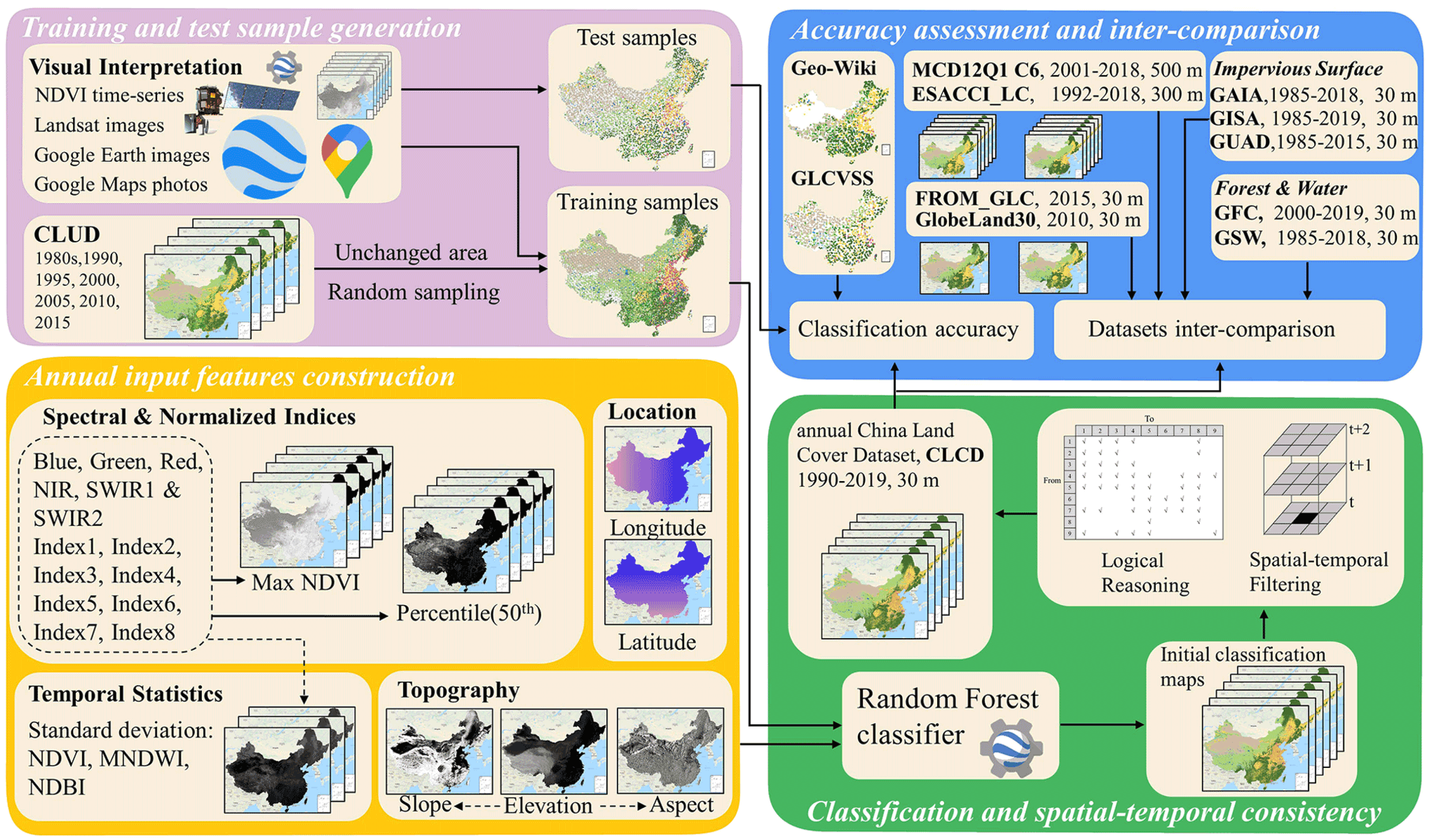
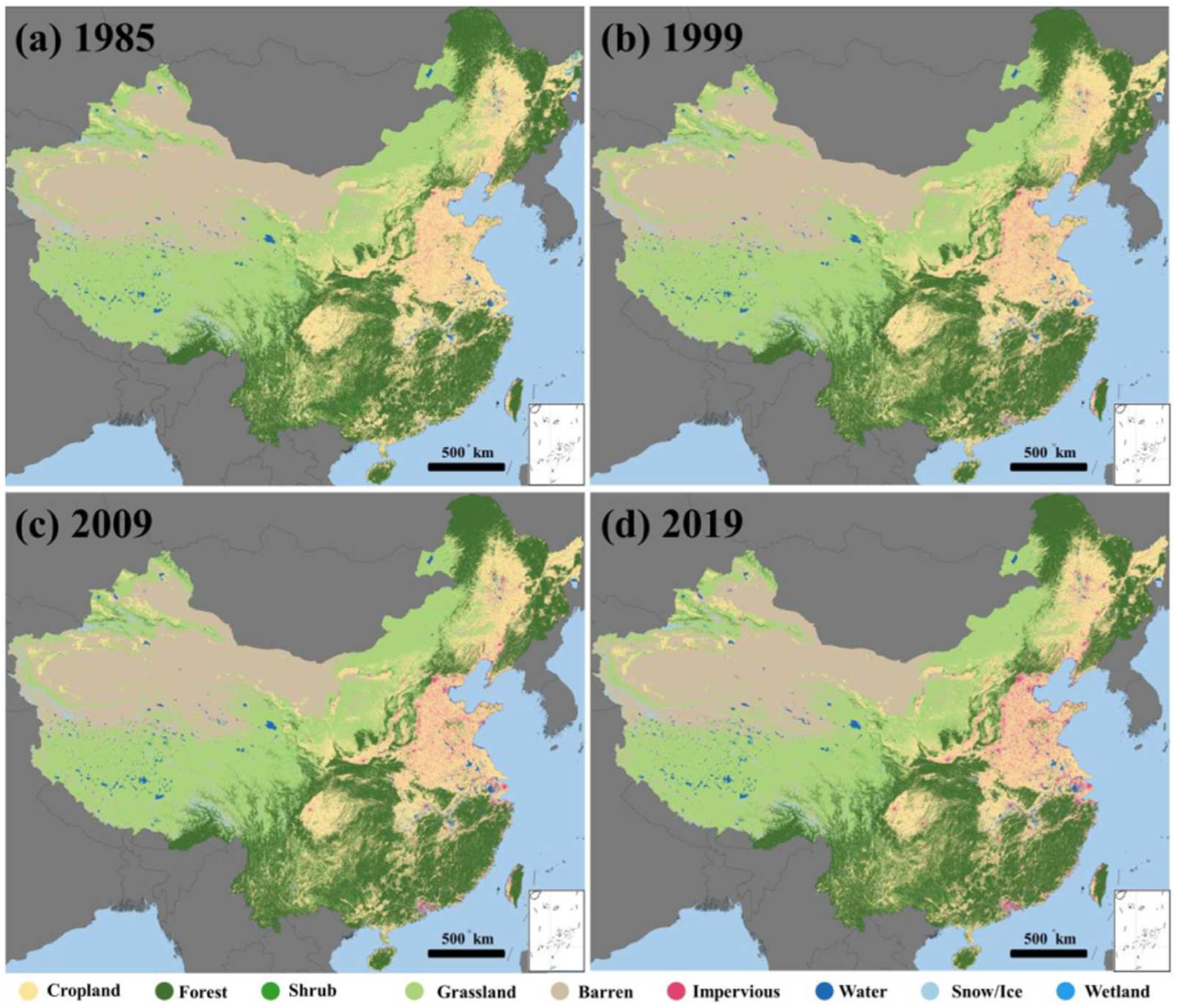
2.3.2. Regarding the Adoption of CLUD Data Explanation

There are four reasons for using CLUD dataset to calculate the carbon sink: First, this dataset checks the land use CLUD dataset with the relevant data of the National Bureau of Statistics, provincial statistics bureaus, and municipal statistics bureaus. Although there are differences in the data, the differences in forest area in most cities and provinces are not significant. Second, the greatest advantage of these data is the continuity of the data in the time series. The research in this paper designs dynamic emission factors and requires continuous time series data. Third, the dataset is relatively complete and includes all cities. These data include data from 333 prefecture-level cities across the country. Due to the influence of other data in this paper, only 282 prefecture-level cities are used. However, there are many missing land use data in the statistics bureaus of each city, and the Ministry of Land and Resources divides land use types into 12 first-level categories such as cultivated land, garden land, forest land, and grassland, which are not conducive to calculating the carbon sink in this paper. Fourth, the data have high publicity and accessibility. Usually, the data of the previous year are updated in August each year. These data are released based on the Google Earth Engine platform and have been updated to 2022, which is more suitable for the research and use of this paper.

In addition, some scholars directly use the forest land and grassland from the statistics bureau to calculate the carbon sink, while ignoring the carbon sink from other land uses. From the calculation results, the carbon sink (carbon coefficient) is less than one-tenth of the carbon emissions, and the carbon sink is mainly concentrated in forest land and grassland. If it is applied to the provincial level, it basically does not affect the results. However, in some cities with high coverage rates of forests, forest land, cultivated land, and water areas, the carbon sink exceeds the carbon emissions. Calculating solely based on forest land and grasslands can lead to significant discrepancies.

2.3.3. Carbon Footprint Accounting Based on Carbon Sinks

China’s main land structure is dominated by cultivated land, forest land and grassland, among which cultivated land accounts for about 35%, forest land accounts for about 38%, and grassland accounts for about 15%. From the perspective of the CLUD dataset, the land use types can be divided into cultivated land, forest, grassland, water area, wasteland and others (including impervious surface, shrub, wetland and snow and ice land), etc. The sum of cultivated land, forest, grassland, water area and wasteland in the CLUD data accounts for about 95%, and the others account for about 5%. Among the others, the impervious surface mainly refers to urban buildings, factories, cement, etc., accounting for 5.2% of the total area and 95% of the others. These lands may have very weak or no carbon absorption capacity, and the carbon sink can be ignored. Therefore, we calculate the carbon sink based on five types of land use: cultivated land, forest, grassland, water area and wasteland. The specific carbon sink accounting equation is as follows:

$$\mathrm{C}{\mathrm{L}}_{\mathrm{i}}=\sum _{\mathrm{i}=1}^5\left(\mathrm{F}{\mathrm{A}}_{\mathrm{i}}\times \mathrm{F}{\mathrm{C}}_{\mathrm{i}}\right),\mathrm{i}=1,2,\cdots ,5$$

(23)

Here, ${\mathrm{C}\mathrm{L}}_{\mathrm{i}}$ represents the CO₂ absorption of the $\mathrm{i}$-th type of land, $\mathrm{F}{\mathrm{A}}_{\mathrm{i}}$ represents the $\mathrm{i}$-th type of land in the land classification. $\mathrm{F}{\mathrm{C}}_{\mathrm{i}}$ represents the carbon sequestration rate per unit area of the $\mathrm{i}$-th type of land. In this paper, it refers to five types of land, namely cultivated land (or farmland), forest land (or forest), grassland, water area and wasteland (or unused land), respectively.

Table 2. Carbon sink coefficient of each land use type (unit: t/hm²∙a).

Researcher	Carbon Sink Coefficient of Cultivated Land	Carbon Sink Coefficient of Forest	Carbon Sink Coefficient of Grassland	Carbon Sink Coefficient of Water Area	Carbon Sink Coefficient of Wasteland
Wang Xiulan (1996) [57]	-	3.81	0.91	-	-
He Yong (2006) [58]	0.69	-	-	-	-
Fang Jingyun (2007) [59]	-	5.77	-	-	0.002
Zhao Rongqin (2013) [60]	0.22	-	0.95	0.46	-
Sun He (2015) [61]	0.42	-	-	0.28	-
Li Lu (2019) [62]	0.13	-	-	-	-
Li Yuanyuan (2023) [63]	0.42	0.64	0.021	0.25	0.005
Mean Value	0.38	4.79	0.93	0.33	0.0036

shows the carbon sink coefficient of each land use type.

Here, the unit of soil erosion is t, and the unit of soil erosion modulus is t/hm² × a, which is the amount of erosion per square kilometer per year. hm² means hectares, and a means year (annual).

Discrepancies in carbon sink coefficients exist due to the variation in research methods and objects among different researchers. We reference the average values reported by each researcher as the basis for the carbon sink coefficients used in this paper. However, coefficients that are significantly high or low are not included in the sample for calculating the average value. Furthermore, with the advancement of agricultural technology, the carbon sink of cultivated land has also undergone certain changes. Therefore, the average value is not used as the basis for calculation, but rather for analysis and reference only.

Regarding the carbon emissions and absorption of cultivated land, we adopt the following equation based on the research outcomes of Tian Yun (2012) and Li Qiang (2022) for calculation [64,65]:

$$\mathrm{C}\mathrm{A}\mathrm{E}=\sum _{\mathrm{i}=1}^{\mathrm{n}}{\mathrm{T}}_{\mathrm{i}}\times {\mathsf{\beta }}_{\mathrm{i}}\times {\displaystyle \frac{{\mathrm{R}}_{\mathrm{i}}}{\mathrm{T}\mathrm{e}}}$$

(24)

Here, $\mathrm{C}\mathrm{A}\mathrm{E}$ is the total carbon emission from cultivated land use, ${\mathrm{T}}_{\mathrm{i}}$ is the quantity of the $\mathrm{i}$-th type of carbon source in cultivated land, ${\mathsf{\beta }}_{\mathrm{i}}$ is the carbon emission coefficient of the $\mathrm{i}$-th type of carbon source in cultivated land, ${\mathrm{R}}_{\mathrm{i}}$ is the carbon source conversion coefficient, $\mathrm{T}\mathrm{e}$ is the technological progress, and $\mathrm{n}$ is the type of cultivated land. Due to technological progress promoting agricultural modernization and improving agricultural efficiency, the resulting carbon emissions are reduced.

$$\mathrm{C}\mathrm{A}\mathrm{A}={\displaystyle \frac{{\sum }_{\mathrm{i}=1}^{\mathrm{n}}{\mathrm{S}}_{\mathrm{i}}\times \mathsf{\gamma }}{{\mathrm{h}}_{\mathrm{i}}}}$$

(25)

Here, $\mathrm{C}\mathrm{A}\mathrm{A}$ is the carbon absorption amount of cultivated land, ${\mathrm{S}}_{\mathrm{i}}$ is the yield of the $\mathrm{i}$-th type of crop, ${\mathsf{\gamma }}_{\mathrm{i}}$ is the carbon absorption rate of the $\mathrm{i}$-th type of crop, ${\mathrm{h}}_{\mathrm{i}}$ is the economic coefficient of the $\mathrm{i}$-th type of crop, and $\mathrm{n}$ is the type of crop. The economic coefficients and carbon absorption rates of the main crops in cultivated land are as follows:

$$\mathrm{N}\mathrm{C}\mathrm{A}=\mathrm{C}\mathrm{A}\mathrm{A}-\mathrm{C}\mathrm{A}\mathrm{E}=\mathrm{A}\mathrm{A}\times {\mathsf{\omega }}_{\mathrm{t}}$$

(26)

$${\mathsf{\omega }}_{\mathrm{t}}={\displaystyle \frac{\mathrm{N}\mathrm{C}{\mathrm{A}}_{\mathrm{t}}}{\mathrm{A}{\mathrm{A}}_{\mathrm{t}}}}$$

(27)

Here, $\mathrm{N}\mathrm{C}\mathrm{A}$ represents the net carbon sink of cultivated land. When $\mathrm{N}\mathrm{C}\mathrm{A}>0$, it indicates that the carbon absorption amount is greater than the carbon emission amount, that is, carbon surplus; when $\mathrm{N}\mathrm{C}\mathrm{A}<0$, it indicates that the carbon absorption amount is less than the carbon emission amount, that is, carbon deficit; when $\mathrm{N}\mathrm{C}\mathrm{A}=0$, it indicates that the carbon absorption amount is equal to the carbon emission amount, that is, carbon neutrality. $\mathrm{A}\mathrm{A}$ represents the area of cultivated land, and $\mathrm{t}$ is the average carbon absorption amount of cultivated land in the $\mathrm{t}$-th year. Due to the improvement of agricultural technology and the reduction in carbon emissions, and when the unit absorption amounts of various crops remains unchanged, the net carbon sink in each year will also change. Therefore, it is obviously not in line with the actual situation to adopt a fixed carbon absorption coefficient. Therefore, in view of the research results of Li Qiang (2022), based on dividing the national net carbon sink of cultivated land by the national cultivated land area, the average annual carbon absorption coefficient of cultivated land is obtained [65].

Table 3. Carbon sink coefficients of cultivated land from 2006 to 2021.

Year	2006	2007	2008	2009	2010	2011	2012	2013
Carbon Sink Coefficient of Cultivated Land	0.31	0.31	0.33	0.34	0.36	0.39	0.41	0.43
Year	2014	2015	2016	2017	2018	2019	2020	2021
Carbon Sink Coefficient of Cultivated Land	0.44	0.46	0.41	0.42	0.44	0.46	0.49	0.50

shows the carbon sink coefficients of cultivated land from 2006 to 2021.

2.3.4. Ecological Carrying Capacity Based on Carbon Sinks

The Carbon Ecological Carrying Capacity (CECC) is an indicator that measures the ability of an ecosystem in a region to absorb and store carbon while maintaining ecological balance and human well-being. The carbon-based ecological carrying capacity pays special attention to the carbon sequestration capacity of the ecosystem for CO₂ in the atmosphere. Natural ecosystems such as forests, grasslands, and wetlands absorb CO₂ through natural processes such as photosynthesis and convert it into organic matter, thereby reducing the content of greenhouse gases in the atmosphere and enabling the regional ecosystem to achieve stability and good carrying capacity.

Many scholars’ research on carbon-based ecological carrying capacity has also continued to deepen. The carbon-based ecological carrying capacity index designed in this article draws on the research of Lu Junyu (2012) and Li Yuanyuan (2023), extending the concept of ecological carrying capacity in traditional ecology, aiming to measure the proportional relationship between carbon emissions and carbon absorption in different regions [63,66]. First, calculate the ratio of the carbon sink amount (that is, the carbon absorption amount) to the total national carbon sink capacity; then, calculate the ratio of the carbon emissions of each region to the total national emissions, and finally calculate the ratio of the carbon sink to the carbon emissions.

$$\mathrm{C}\mathrm{E}\mathrm{C}{\mathrm{C}}_{\mathrm{i}}={\displaystyle \frac{\frac{\mathrm{C}\mathrm{A}{\mathrm{A}}_{\mathrm{i}}}{\mathrm{C}\mathrm{A}\mathrm{A}}}{\frac{\mathrm{C}\mathrm{A}{\mathrm{E}}_{\mathrm{i}}}{\mathrm{C}\mathrm{A}\mathrm{E}}}}$$

(28)

Here, $\mathrm{C}\mathrm{E}\mathrm{C}{\mathrm{C}}_{\mathrm{i}}$ is the carbon sink ecological carrying capacity of region $\mathrm{i}$, $\mathrm{C}\mathrm{A}{\mathrm{A}}_{\mathrm{i}}$ represents the carbon sink amount of region $\mathrm{i}$, $\mathrm{C}\mathrm{A}\mathrm{A}$ represents the total carbon sink amount, $\mathrm{C}\mathrm{A}{\mathrm{E}}_{\mathrm{i}}$ represents the carbon emission amount of region $\mathrm{i}$, and $\mathrm{C}\mathrm{A}\mathrm{E}$ represents the total carbon emission amount of all regions.

If $\mathrm{C}\mathrm{E}\mathrm{C}\mathrm{C}>1$, it indicates that the contribution of carbon absorption in this region is greater than the contribution of carbon emissions; that is, it has a relatively high ecological capacity. If $\mathrm{C}\mathrm{E}\mathrm{C}\mathrm{C}<1$, it indicates that the contribution of carbon absorption in this region is less than the contribution of carbon emissions; that is, it has a relatively low ecological capacity and is prone to the formation of the greenhouse effect.

3. Analysis and Conclusion of Carbon Footprint-Accounting Results

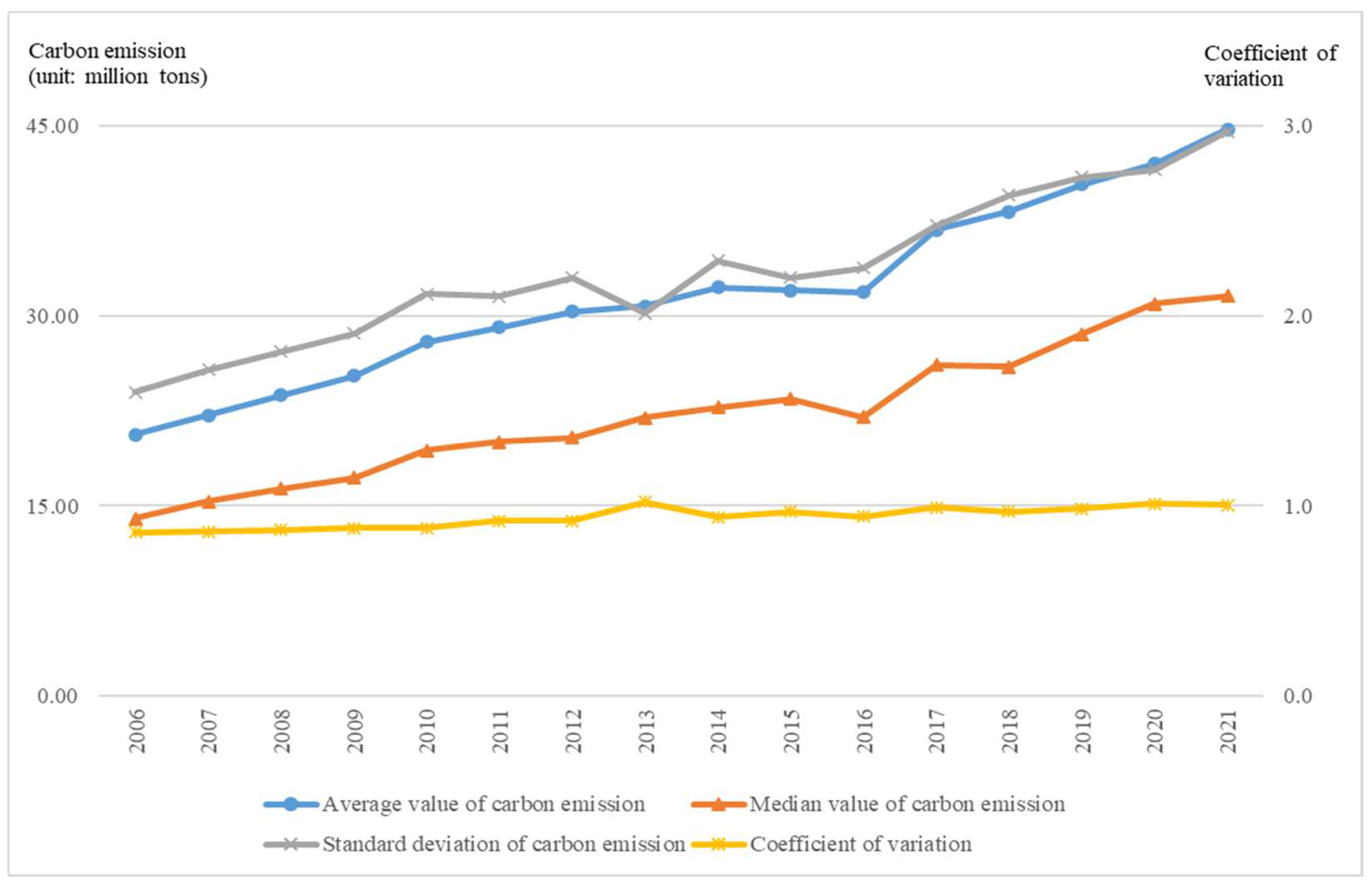
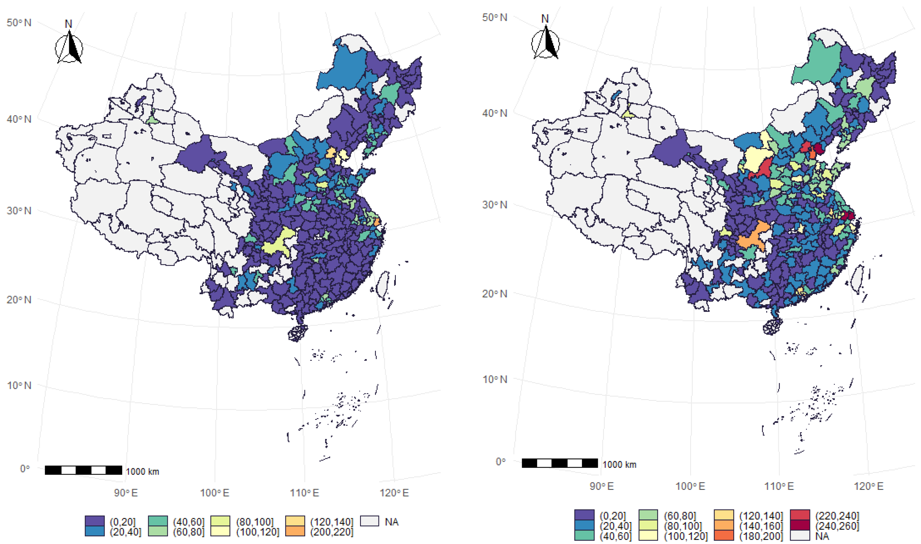
3.1. Estimation and Analysis of Urban Carbon Footprint Based on Emission Factor Method

In China, the rapid development of urban agglomerations has become an important engine for economic growth, but at the same time, it has also brought about carbon emission problems that cannot be ignored. There are seven major urban agglomerations that include the Yangtze River Delta, Beijing–Tianjin–Hebei, the Pearl River Delta, the Middle Reaches of the Yangtze River, Chengdu–Chongqing, the Central Plains, and the Guanzhong Plain. Among them, the Yangtze River Delta urban agglomeration includes 25 cities: Nanjing, Wuxi, Changzhou, Suzhou, Nantong, Yancheng, Yangzhou, Zhenjiang, Taizhou, Hangzhou, Ningbo, Jiaxing, Huzhou, Shaoxing, Jinhua, Zhoushan, Taizhou, Hefei, Wuhu, Ma’anshan, Tongling, Anqing, Chuzhou, Chizhou, and Xuancheng; the Pearl River Delta urban agglomeration includes 9 cities: Guangzhou, Shenzhen, Zhuhai, Foshan, Huizhou, Dongguan, Zhongshan, Jiangmen, and Zhaoqing; the Beijing–Tianjin–Hebei urban agglomeration includes 14 cities, including Baoding, Tangshan, Langfang, Shijiazhuang, Qinhuangdao, Zhangjiakou, Chengde, Cangzhou, Hengshui, Xingtai, Handan, and Anyang; the urban agglomeration in the Middle Reaches of the Yangtze River includes 11 cities: Wuhan, Yichang, Jingzhou, Huangshi, Changsha, Yueyang, Zhuzhou, Xiangtan, Nanchang, Jiujiang, and Ganzhou; the Chengdu–Chongqing urban agglomeration includes 15 cities: Chengdu, Zigong, Luzhou, Deyang, Mianyang, Suining, Neijiang, Leshan, Nanchong, Meishan, Yibin, Guang’an, Dazhou, Ya’an, and Ziyang; the urban agglomeration in the Central Plains includes 15 cities: Zhengzhou, Kaifeng, Luoyang, Pingdingshan, Xinxiang, Jiaozuo, Xuchang, Luohe, Jiyuan, Hebi, Shangqiu, Zhoukou, Jincheng, Bozhou, Liaocheng, and Heze; the Guanzhong Plain urban agglomeration includes 11 cities: Xi’an, Baoji, Tongchuan, Weinan, Yangling, Shangluo, Tianshui, Pingliang, Qingyang, Yuncheng, and Linfen. These urban economic circles, with their huge economic scale and population base, have a profound impact on the regional and even the national carbon footprint.

As shown in Figure 3, From 2006 to 2021, the data of the carbon emissions of 278 prefecture-level cities across the country show that the average annual emissions of nitrogen dioxide rose from 2063 tons to 4477 tons, with an increase of 117% during the period, reflecting the overall growth trend of carbon emissions, while the median increased from 1399 tons to 3159 tons, indicating that the carbon emissions of more than half of the cities have increased. The fluctuation range of the standard deviation gradually increased. When the overall coefficient of variation (that is, the average value divided by the standard deviation) is always close to 1, it indicates that the fluctuation range of carbon emissions relative to the average level remains at a high level, which may be related to the economic development level, industrial structure, and energy consumption patterns of different cities.

As shown in Figure 4, from 2006 to 2021, the carbon emissions of the seven major urban agglomerations in China showed different trends. The average carbon emissions of the three major urban agglomerations of the Yangtze River Delta, the Pearl River Delta, and the Beijing–Tianjin–Hebei region increased rapidly, rising from 2948 tons, 3588 tons, and 3736 tons to 6611 tons, 7486 tons, and 7856 tons, respectively, with an increase of more than 100%. This indicates the expansion of economic activities and the high demand for energy in the Yangtze River Delta, the Pearl River Delta, and the Beijing–Tianjin–Hebei region. Among them, the carbon emissions of the Pearl River Delta urban agglomeration decreased in 2015 and then rebounded rapidly, reflecting the characteristics of the manufacturing and export-oriented economy. The Beijing–Tianjin–Hebei urban agglomeration adopted emission reduction measures from 2012 to 2016, resulting in a slow growth in carbon emissions. Subsequently, with economic development and energy demand, carbon emissions continued to rise. The carbon emissions of the urban agglomerations in the Middle Reaches of the Yangtze River, the Guanzhong Plain, and the Central Plains increased relatively steadily. The total amount of and increase in carbon emissions in the Chengdu–Chongqing region were both relatively low, indicating that there are a large number of water resources in the Chengdu–Chongqing region or the southwest of China; hydropower generation is more widespread, and the economic development is greener compared to other urban agglomerations. In conclusion, the changes in carbon emissions of each urban agglomeration reflect the differences in regional economic development models and energy consumption structures, and green development and low-carbon transformation should be treated differently.

As shown in Figure 5, from the data of the coefficient of variation, the coefficient of variation of carbon emissions in the Yangtze River Delta urban agglomeration is relatively stable, remaining at around 0.3, indicating that the fluctuation of carbon emissions in the Yangtze River Delta is small, and the difference in carbon emissions among prefecture-level cities within the region is relatively balanced. The variation coefficients of the Pearl River Delta and the Central Plains urban agglomerations fluctuate between 0.5 and 0.6, respectively, indicating that the differences among prefecture-level cities within these regions are also relatively small. On the other hand, the variation coefficients of the urban agglomerations in the Middle Reaches of the Yangtze River, Chengdu–Chongqing, and Guanzhong Plain fluctuate between 1 and 2, reflecting significant fluctuations in carbon emissions over the years in these regions, which may be related to the layout of heavy industry and the adjustment of the energy structure within the region. However, the overall downward trend within the region indicates that the differences among cities are narrowing. The variation coefficient of the Beijing–Tianjin–Hebei urban agglomeration ranges from 0.75 to 1.02, indicating a large difference in carbon emissions among prefecture-level cities within the region, and this difference has persisted.

In conclusion, taking the Beijing–Tianjin–Hebei urban agglomeration as an example, its industrial structure is heavy, energy consumption is high, and carbon emission density is high. Shanghai, as the core of the Yangtze River Delta urban agglomeration, has developed finance and service industries, and economic growth leads to a large energy demand. The Pearl River Delta urban agglomeration has high total carbon emissions due to its dense manufacturing industry and strong energy demand. The urban agglomeration in the Middle Reaches of the Yangtze River covers a vast area, and the process of industrialization and urbanization is accelerating, resulting in rapid growth in the carbon footprint. The Central Plains urban agglomeration and the Guanzhong Plain urban agglomeration, as emerging regions, have also seen an increase in carbon emissions. Although the Chengdu–Chongqing urban agglomeration is relying on the Western Development Strategy and is becoming a new economic growth point, it is rich in water resources, and hydropower generation provides sufficient energy supply, resulting in relatively slow growth in overall carbon emissions, and is a classic representative of green development. In general, each urban agglomeration needs to take effective measures to optimize the industrial structure, improve energy efficiency, promote low-carbon technological innovation, and jointly build a green and sustainable urban agglomeration development model.

3.2. Estimation and Analysis of Urban Carbon Footprint Based on the Adjusted Emission Factor Method

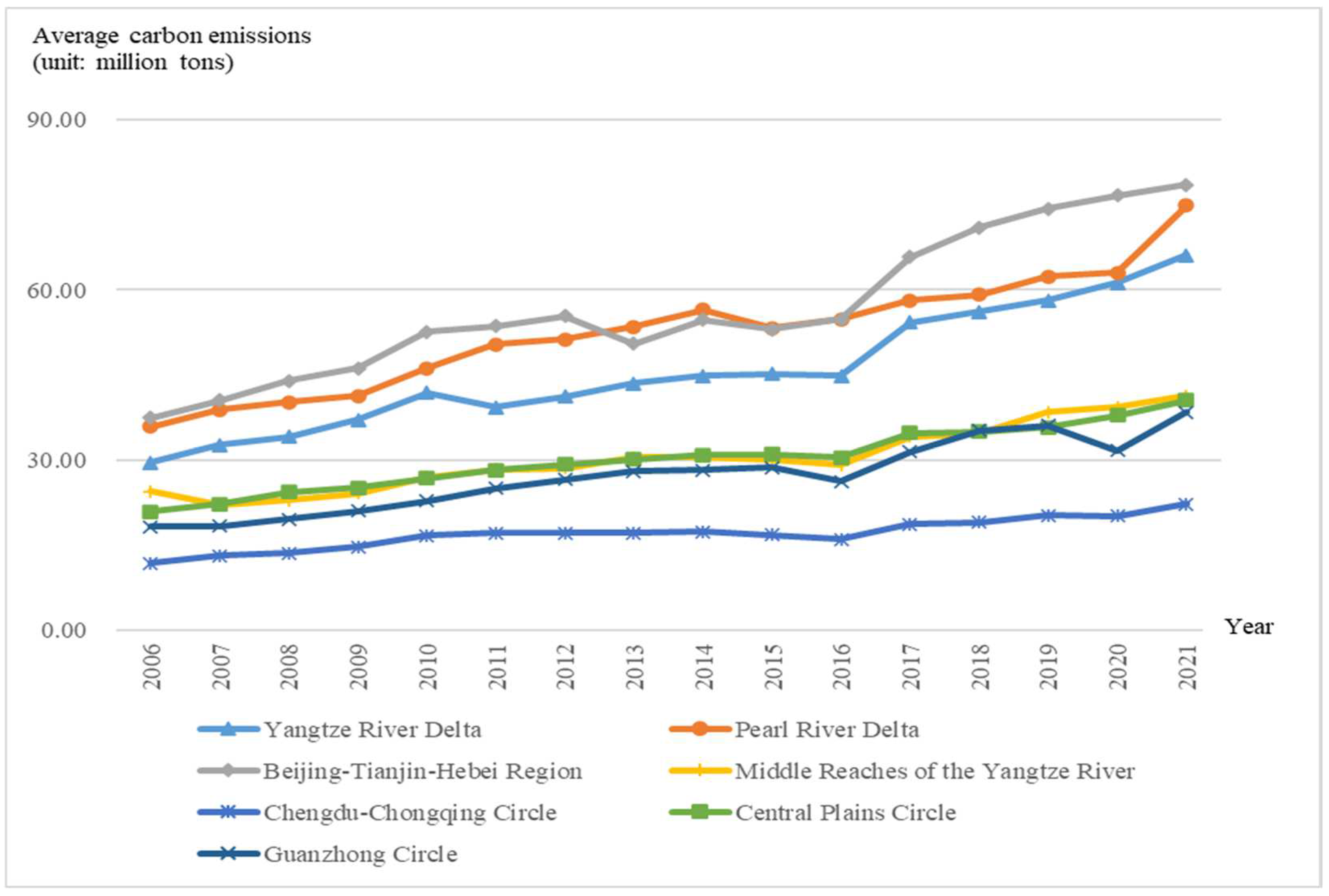
3.2.1. Estimation of Urban Carbon Footprint

Based on the research in Section 3.1, this study adopted the same accounting method and data sources to conduct an in-depth analysis of the carbon footprints of 282 prefecture-level cities. By introducing the adjustment of dynamic emission factors, we can more accurately reflect the carbon emission situation of each city in different years. The adjustment of dynamic emission factors takes into account factors such as technological progress, changes in energy structure, and policy influences, all of which may have a significant impact on the carbon emissions of cities.

Through the adjustment of dynamic emission factors, we found that the carbon footprints of some cities showed a downward trend, which may be attributed to the energy conservation and emission reduction measures taken by the local government, the promotion and use of clean energy, and the innovative application of green technologies. However, the carbon footprints of some cities are still relatively high, which reminds us that in the future urban development, we need to further strengthen environmental protection and sustainable development strategies. In general, through the precise accounting method and the adjustment of dynamic emission factors, it provides a comprehensive and objective perspective to examine the current situation of carbon footprints of prefecture-level cities in China and provides a scientific basis for urban carbon emission management.

As shown in Figure 6, judging from the changes in the color of the map, in 2006, the carbon emissions of the vast majority of cities were below 20 million tons, and the maximum carbon emission was 113.81 million tons in Tangshan, Hebei Province. With economic development, at least half of the cities had carbon emissions of more than 40 million tons in 2021. The maximum carbon emission was 258.96 million tons in Suzhou, Jiangsu Province, mainly due to the influence of economic development. The second was 240.32 million tons in Tangshan, Hebei Province, mainly caused by thermal power generation, and the third was 230.13 million tons in Yulin, Shaanxi Province, mainly caused by coal mining, etc. (The above rankings do not include the carbon emission data of municipalities directly under the Central Government). In addition, by comparing the two maps, it can be seen that the carbon emissions of eastern coastal cities have increased significantly; in particular, the colors of cities around the Yangtze River Delta and the Beijing–Tianjin–Hebei region have darkened significantly, and the carbon emissions have increased significantly.

However, it is worth noting that the four municipalities directly under the Central Government, namely Beijing, Tianjin, Shanghai, and Chongqing, due to their large scale and size, may introduce large errors in the carbon footprint accounting within the region. In order to improve the accuracy and reliability of further analysis and research, the method and data of the carbon footprint accounting of the above 282 cities are still used, as well as the carbon footprint of the cities after the adjustment of dynamic emission factors, but the data of these four municipalities directly under the Central Government are excluded in the research and analysis process.

As shown in

Table 4. Adjusted average carbon emissions per city in seven major economic circles (unit: million tons).

	Economic Circle	Yangtze River Delta	Central Plains Circle	Guanzhong Circle	Pearl River Delta	Beijing–Tianjin–Hebei	Middle Reaches of Yangtze River	Chengdu–Chongqing Circle
Year
2006		31.2	20.8	18.1	35.9	37.4	24.5	11.7
2007		31.9	21.7	18.4	38.5	39.9	21.8	12.9
2008		34.4	23.1	19.2	39.6	42.1	22.4	12.5
2009		37.1	23.4	20.4	40.4	43.7	23.4	13.4
2010		40.4	24.7	21.6	44.9	48.9	25.7	14.8
2011		41.6	25.8	22.9	48.8	49.2	26.1	15.1
2012		42.8	26.3	23.3	49.5	50.4	25.7	15.1
2013		40.7	26.7	24.5	51.4	45.9	27.2	15.0
2014		41.8	27.4	24.7	54.1	49.1	26.8	15.0
2015		41.8	27.4	24.7	50.8	46.7	26.7	14.4
2016		41.1	26.6	22.2	52.0	47.5	25.8	13.6
2017		49.1	29.7	26.1	54.7	55.9	29.7	15.5
2018		50.7	29.8	29.0	55.4	60.1	29.9	15.6
2019		52.3	30.2	29.6	58.3	62.7	33.0	16.7
2020		54.9	31.8	25.4	58.8	64.4	33.5	16.2
2021		59.1	34.1	31.4	70.0	65.9	35.4	18.0

, the data show that the carbon emissions of most economic circles show an upward trend, which may be related to economic growth, the industrialization process, and the increase in energy consumption.

The carbon emissions of the Yangtze River Delta economic circle increased from 31.2 million tons in 2006 to 59.1 million tons in 2021, showing significant growth, reflecting the expansion of economic activities in this region. The emissions of the Pearl River Delta economic circle also increased from 35.9 million tons to 70.0 million tons, with a significant increase. This may be related to the characteristics of the manufacturing and export-oriented economy in this region.

The carbon emissions of the Beijing–Tianjin–Hebei economic circle showed an upward trend before 2013 and then decreased. This may be related to the environmental protection policies and energy structure adjustment implemented in this region. The carbon emissions of the Central Plains circle and the Guanzhong circle increased relatively steadily, while the growth rate of the Chengdu–Chongqing circle was relatively fast, increasing from 11.7 million tons to 18.0 million tons. It is worth noting that the carbon emissions of the Middle Reaches of the Yangtze River economic circle decreased after 2015, which may be related to the efforts in energy efficiency improvement and the use of clean energy in this region. However, the emissions of this economic circle increased again in 2020, which may be affected by special reasons such as the epidemic.

Overall, the changing trend of carbon emissions in each economic circle reflects the differences in economic development models and energy consumption structures in different regions of China. Although the CO₂ emissions adjusted only by green technology have decreased, the overall trend and changes have a certain correlation with those before the adjustment.

Among the 97 prefecture-level cities in the seven major economic circles, 11 provincial capital cities were selected to analyze and study the carbon emissions of each provincial capital city after the adjustment of the dynamic emission factor. The details are shown in Figure 7.

The data show that between 2006 and 2021, the CO₂ emissions of most cities showed a year-on-year growth trend, which is closely related to China’s rapid industrialization and urbanization process. Cities in the Yangtze River Delta economic circle, represented by Nanjing and Hangzhou, as well as Guangzhou, the core of the Pearl River Delta, have high CO₂ emissions, reflecting the intensity of economic activities and the scale of energy consumption in these regions, especially Nanjing, whose emissions increased from 75.31 million tons in 2006 to 139.9 million tons in 2021. The emissions of Nanchang and Changsha have been relatively stable after 2015, which may be related to the active efforts of local governments in energy conservation and emission reduction. However, for cities like Shijiazhuang, although the emissions were 69.21 million tons in 2006 and increased to 95.59 million tons in 2021, the growth rate has slowed down in recent years, which may be related to the strengthening of environmental protection policies and the adjustment of the energy structure. In addition, the growth of CO₂ emissions in Chengdu in the Chengdu–Chongqing circle and Xi’an in the Guanzhong circle is also significant, which is consistent with the rapid economic development of these two cities in recent years.

Although the CO₂ emissions of most cities show an upward trend, some cities show different changing trends, which also reveal the effects of their respective development models and environmental protection measures. For example, the emissions of Zhengzhou increased from 42.92 million tons in 2006 to 69.95 million tons in 2021, showing a relatively fast growth rate, which may be related to its status as a transportation hub and a large population city. Wuhan, as an important city in the urban agglomeration in the Middle Reaches of the Yangtze River, its emissions increased from 68.47 million tons in 2006 to 103.11 million tons in 2021, and the growth rate is also relatively fast.

Overall, the total amount of CO₂ emissions indicates that while China is pursuing economic growth, it is also facing challenges in environmental protection and climate change. The governments of various economic circles actively promote environmental protection policies and adopt different emission reduction measures, resulting in continuous technological innovation, optimization of energy structure and energy efficiency within each economic circle, thereby promoting the application of green and low-carbon technologies, reducing greenhouse gas emissions, and promoting the construction of ecological civilization. At the same time, the enhancement of public environmental awareness and the realization of the transformation of green lifestyles and consumption patterns have jointly made many contributions to mitigating climate change.

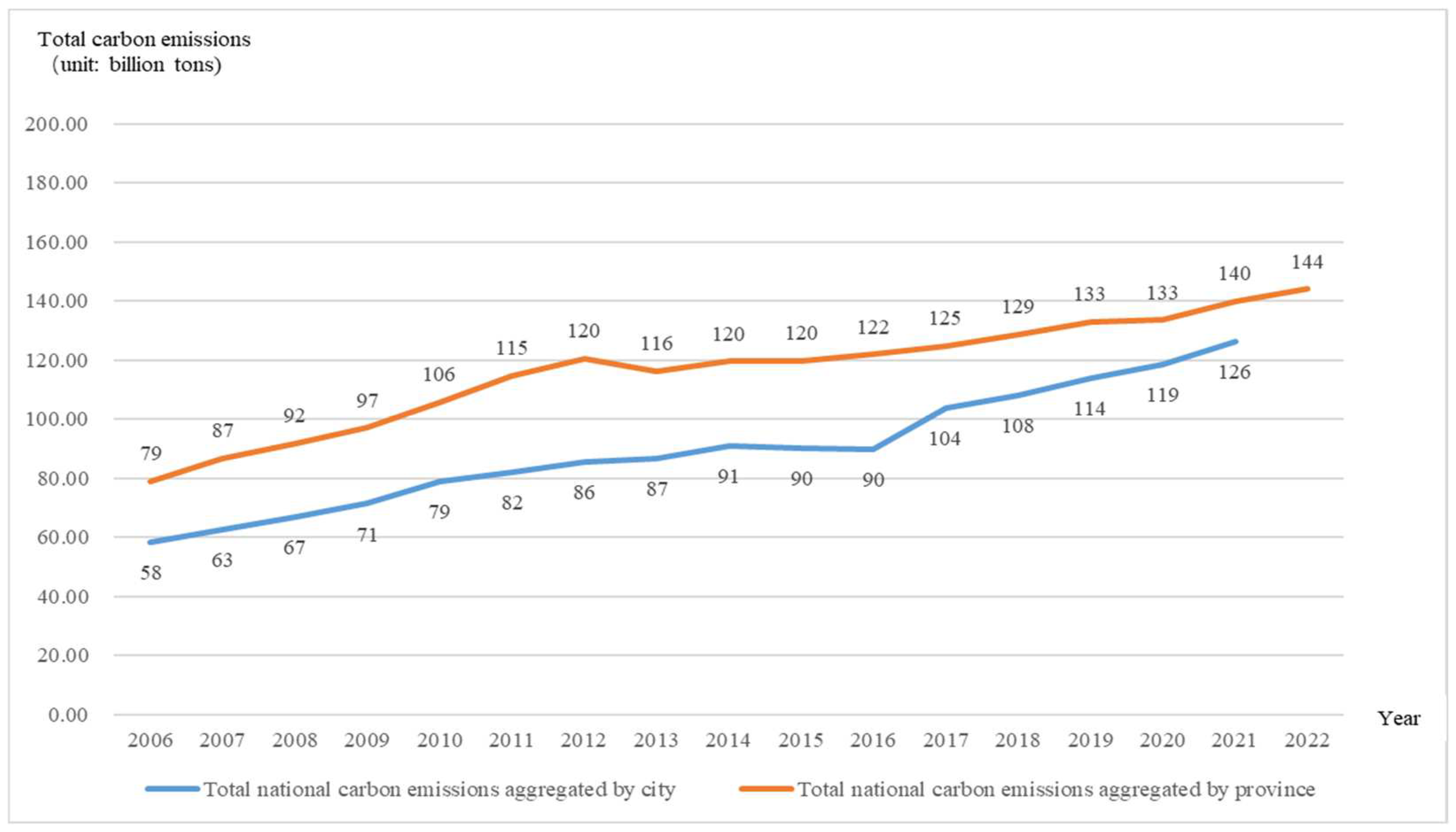
3.2.2. Estimation and Validation of Provincial Carbon Footprint

The most straightforward way to assess the carbon footprint of each province is to add and aggregate the carbon emission data of the prefecture-level cities. By collecting data on energy consumption statistics, industrial production activities, transportation emissions, and residents’ lives, the carbon emissions of each city in one year are calculated, and then the carbon emissions of all cities in the province are accumulated or summed to reflect the total carbon footprint of the province. The advantage of this method is the locality and specificity of the data. However, this method also has its limitations. There may be differences in data collection standards between cities, and provincial-level energy flows and carbon emissions may be ignored in the aggregation process. In view of the original data source of the statistical yearbook, it is also found that some urban data are missing in the National Statistical Yearbook and have not been counted. In this article, 282 prefecture-level cities are mentioned, but there are actually 333 prefecture-level cities in total. Therefore, we use the provincial level as the original data source statistical unit to recalculate the carbon footprint in the provincial-level region.

As shown in Figure 8, the data show that there are differences in the total amount of carbon dioxide emissions obtained through the two methods of city aggregation and provincial aggregation (neither of which includes Lhasa Autonomous Region and its sub-prefecture-level cities). The city aggregation method increased from 5.80 billion tons to 12.60 billion tons, while the provincial aggregation method increased from 7.90 billion tons to 14.40 billion tons. This difference can be caused by a number of factors, including missing city data, inconsistent standards for data collection and reporting, energy flows between provinces and cities, and differences in statistical methods at different levels of government. The city aggregation method may focus more on direct energy consumption and carbon emission activities, while the provincial aggregation method may include energy distribution across cities and energy conversion losses at the provincial level. Over time, the relative gap between the two methods has gradually narrowed, reflecting improvements in energy management and statistical capabilities.

When calculating the carbon footprint of each province, the dynamic emission factor is still determined according to the above formula of the green technology adjustment coefficient, and the carbon dioxide emissions of each province are adjusted according to the dynamic emission factor. First, the provincial data in the statistical yearbook are more comprehensive than the city data. The period span has been updated from 2006 to 2022, and there are also pollutant emission data. There are not only more comprehensive provincial sulfur dioxide emissions in exhaust gas emissions, but also nitrogen oxide emissions in exhaust gas emissions. There is chemical oxygen demand in wastewater emissions and other data. The second three indicators are used as the base layer of the green technology adjustment factor. In order to more accurately identify the green technology adjustment factor, the entropy weight is calculated using three indicators such as sulfur dioxide emissions per standard amount of coal consumed, nitrogen oxide emissions per standard amount of coal consumed, and chemical oxygen demand per standard amount of coal consumed.

As shown in

Table 5. Calculation results of entropy weight method of three indexes used in green technology adjustment coefficient.

Indicator	Calculation Method	Unit	Abbreviation	Weight	Entropy Value
Unit sulfur dioxide emissions	Total sulfur dioxide emissions/total standard coal consumption	Ton/ten thousand tons	SO2C	0.26	1.00
Unit nitrogen oxide emissions	Total nitrogen oxide emissions/total standard coal consumption	Ton/ten thousand tons	NOXC	0.50	0.99
Unit chemical oxygen demand	Total chemical oxygen demand/total standard coal consumption	Ton/ten thousand tons	O2C	0.24	1.00

, from the results of the entropy weight method, the weights of sulfur dioxide (SO₂C), nitrogen oxides (NO_XC) and chemical oxygen demand (O₂C) emissions per unit of energy consumption are divided into 26%, 50% and 24%, indicating that nitrogen oxides have a greater impact on the index and are relatively more important. The entropy value measures the degree of variation in the index value. The entropy values of SO₂C, NO_XC and O₂C are 1.00, 0.99 and 1.00, respectively, indicating that their data distributions have high consistency and are suitable for use as indicators of the entropy weight method.

The provinces are divided according to the above seven economic circles, of which the Yangtze River Delta economic circle includes Shanghai, Jiangsu, Zhejiang and Anhui; the Middle Reaches of the Yangtze River economic circle include Hunan, Hubei and Jiangxi; the Beijing–Tianjin–Hebei economic circle includes Beijing, Tianjin and Hebei; the Chengdu–Chongqing economic circle includes Sichuan and Chongqing; the Pearl River Delta economic circle refers to Guangdong; the Central Plains economic circle refers to Henan; and the Guanzhong economic circle refers to Shaanxi. The carbon emissions of the economic circle are as follows:

In China’s seven economic circles (fifteen provinces or municipalities directly under the Central Government), the total carbon dioxide emissions rose rapidly from 4.55 billion tons in 2006 to 6.57 billion tons in 2011 and then slowly declined to 6.21 billion tons by 2015. In 2016, China officially joined the Paris Agreement; that same year, seven provinces and cities carried out a carbon emission trading pilot, using market mechanisms to control greenhouse gas emissions and promote enterprise emission reduction, meaning that emissions fell sharply to 4.87 billion tons, but then they gradually rose to 5.80 billion tons by 2022.

Among them, the total carbon dioxide emissions of the four provinces in the Yangtze River Delta economic circle remained increased, rising from 1.31 billion tons in 2006 to 1.79 billion tons in 2015, and then declined after 2016, but eventually slowly rose to 1.84 billion tons in 2022. The total carbon dioxide emissions of the three provinces in the Beijing–Tianjin–Hebei economic circle rose from 870 million tons in 2016 to 1.20 billion tons in 2015, and remained between 1 and 1.10 billion tons in subsequent years. The Pearl River Delta economic circle rose from 540 million tons in 2006 to 790 million tons in 2022. The Middle Reaches of the Yangtze River economic circle rose from 710 million tons in 2006 to 780 million tons in 2022. The overall increase was less and remained relatively stable. Although the total emissions of the Chengdu–Chongqing economic circle and the Central Plains economic circle are relatively low, the overall carbon dioxide emissions remained stable from 2006 to 2022. Whilst the Guanzhong economic circle has the smallest total, due to the rapid development of the regional economy, the total carbon dioxide emissions have risen rapidly from 170 million tons in 2006 to 290 million tons in 2022, an increase of up to 72%.

To sum up, China’s total carbon dioxide emissions in different economic circles basically maintained a slow increase and then remained stable. After being influenced by policies such as the Paris Agreement, emissions fell sharply, and finally, carbon dioxide emissions slowly rebounded. Although emissions have declined in some years and regions, there is still a need to further increase emission reduction efforts as a whole, especially in industrial upgrading, energy structure optimization, clean energy use and technological innovation.

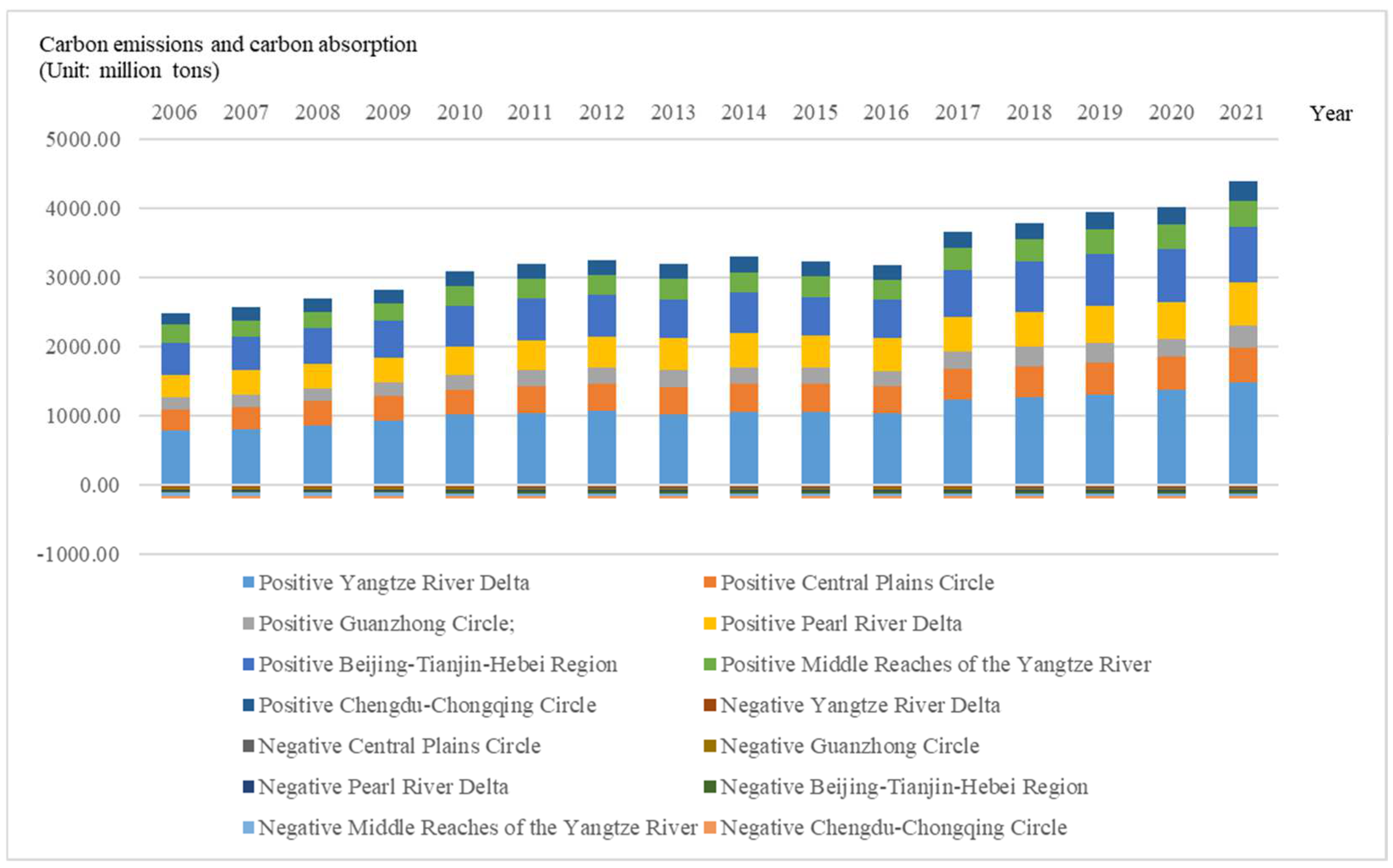
3.3. Estimation and Analysis of Urban Carbon Footprint Based on Carbon Sinks

3.3.1. Estimation of Urban Carbon Sinks

Based on the above research, still using the 282 prefecture-level cities mentioned above as the basic data, the basic data of carbon sinks adopts the CLCD dataset, and the carbon sink absorption coefficient (except for cultivated land) adopts the average value in Table 5 above and does not change over time. The farmland carbon sink absorption coefficient adopts

Table 6. Trends of carbon sinks per city on average in the seven major economic circles (unit: ten thousand tons).

	Economic Circle	Yangtze River Delta	Central Plains Circle	Guanzhong Circle	Pearl River Delta	Beijing–Tianjin–Hebei	Middle Reaches of Yangtze River	Chengdu–Chongqing Circle
Year
2006		135.0	62.6	295.4	164.1	220.7	390.8	201.9
2007		134.6	62.4	296.6	165.3	221.0	390.4	201.7
2008		135.6	64.3	299.1	166.2	224.0	390.7	206.0
2009		135.7	64.8	300.9	166.1	225.6	389.0	206.4
2010		136.5	66.2	303.5	166.3	228.3	388.2	207.8
2011		137.3	67.7	306.8	166.8	231.4	388.7	208.9
2012		137.4	69.0	308.8	167.0	234.1	388.8	210.5
2013		136.4	69.8	310.9	168.7	236.1	388.5	209.8
2014		136.2	70.4	312.5	168.7	237.1	388.0	210.9
2015		136.4	71.5	315.3	168.7	239.0	387.7	213.9
2016		134.5	69.1	313.8	167.8	236.1	384.4	213.9
2017		135.1	70.2	316.1	166.8	237.6	384.7	215.0
2018		135.6	71.3	318.0	166.4	239.6	385.1	216.2
2019		135.8	72.7	320.3	165.9	241.5	385.8	220.4
2020		136.4	74.4	323.4	165.4	243.7	386.6	224.1
2021		136.7	74.9	324.7	165.4	244.4	387.4	225.1

above and changes annually. Since Beijing, Tianjin, Shanghai and Chongqing are municipalities directly under the Central Government with a large scale and volume, they are not included in the calculation within the region.

From 2006 to 2021, the carbon sink data of the seven major economic circles in China showed different growth trajectories and regional characteristics but, overall, remained basically stable. The main reason is that the forest carbon sinks remained basically stable. Among the 282 prefecture-level cities, taking 2021 as an example, the total carbon sink was 976 million tons, of which forest carbon sinks were 832 million tons, accounting for about 85% of the total carbon sink, followed by farmland and grassland carbon sinks of 80 million tons and 62 million tons, respectively.

From the perspective of each economic circle, the carbon sink of cities in the Central Plains circle was relatively small. Due to the continuous efforts in ecological construction and environmental protection, the average growth of urban carbon sinks was close to 20%. The Guanzhong circle, Beijing–Tianjin–Hebei and the Chengdu–Chongqing circle also had certain growth. In addition, the average carbon sink values in the Guanzhong circle and the Middle Reaches of the Yangtze River economic circle were generally higher, which was related to the relatively rich forest and wetland resources in these regions. These natural ecosystems played an important role in absorbing CO₂ in the atmosphere.

From the perspective of the total annual carbon sinks of the seven major economic circles, the total annual carbon sinks of the selected 97 prefecture-level cities are close to 200 million tons. The Middle Reaches of the Yangtze River have rich forest resources and a large number of alternative cities, so the total carbon sink is the highest on the whole, absorbing CO₂ to generate a carbon sink of about 42.66 million tons on average every year over the past 15 years, while the Central Plains circle is mainly composed of plains, and the Pearl River Delta has a developed water system, so the total carbon sink is relatively low.

From the perspective of carbon sink growth during the study period, the Guanzhong circle grew the fastest due to the small carbon sink at the beginning and the continuous efforts in ecological construction and environmental protection, followed by the Guanzhong circle, Beijing–Tianjin–Hebei and the Chengdu–Chongqing circle. Those with slow growth or no growth include the Yangtze River Delta, the Pearl River Delta and the Middle Reaches of the Yangtze River. This may be related to land use in these regions, such as the reduction in forests, farmland or water areas, which is more conducive to economic development. Or it can be said that urban construction land is more economically valuable than forests, farmland or water areas.

To sum up, from 2006 to 2021, the carbon sink data of the seven major economic circles in China showed overall stability, with forest carbon sinks dominating, reaching 85%. Regions such as the Central Plains circle and the Guanzhong circle achieved significant growth through ecological construction, while the growth in the Yangtze River Delta, the Pearl River Delta and the Middle Reaches of the Yangtze River was slower, which may be related to changes in land use. Overall, natural ecosystems have played a key role in promoting regional carbon sink growth.

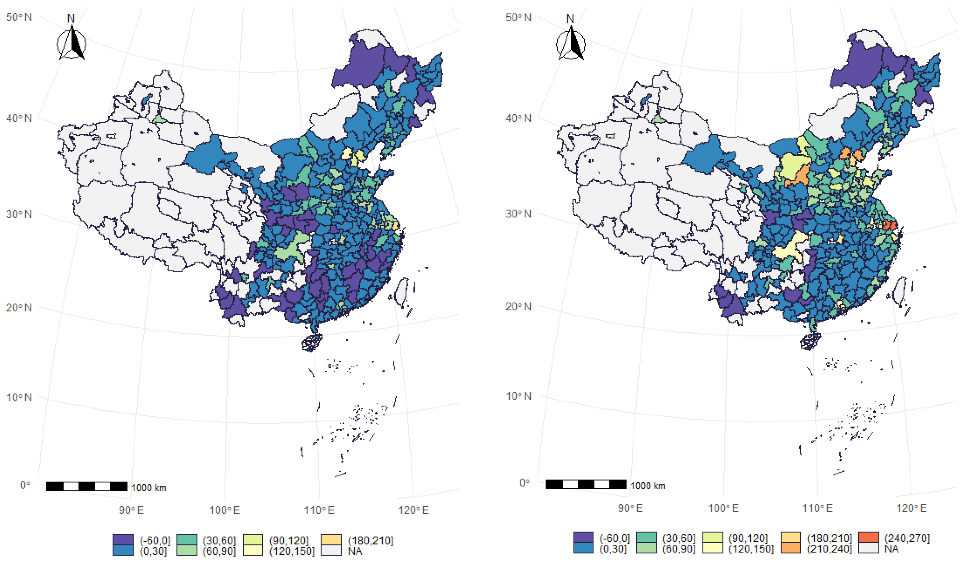
3.3.2. Estimation of Urban Net Carbon Sinks

The urban net carbon sink refers to the total amount of CO₂ absorbed through processes such as photosynthesis of vegetation and soil carbon storage within the urban area minus the amount of CO₂ directly emitted by urban activities. It reflects the net absorption capacity of the urban ecosystem for greenhouse gases in the atmosphere and is an important indicator for assessing the ecological health of cities and responding to climate change. A high net carbon sink means that the city has a better ecological regulation function and helps to slow down global warming. According to the above research, the net carbon sink is carbon absorption minus carbon emission.

In Figure 9, positive values represent carbon emissions, and negative values represent carbon absorption or carbon sinks. The difference between the two represents net carbon sinks. It is not difficult to see from the figure that for the net carbon sinks of cities in the seven major economic circles, overall, carbon emissions are relatively large and carbon absorption is very small. In Figure 10, net carbon sinks are manifested as carbon deficits, mainly due to urban carbon emissions. The reason is that the seven major economic circles all count as medium and large-sized cities with developed economies, while relatively few areas rich in resources such as forests, farmland, grasslands and water areas are counted. Therefore, from the perspective of cities in economic circles, carbon absorption is seriously insufficient, as is shown from Figure 11. This is mainly because cities in the seven major economic circles are dominated by economically leading cities. With the development of these cities’ economies, carbon emissions are high, and carbon absorption mainly comes from forest resources. Therefore, cities with limited forest resources have more serious carbon deficits. To change the carbon deficit, on the one hand, it is necessary to transform the economy towards being green and low-carbon, and on the other hand, it is also necessary to increase the construction of forestry.

In Figure 12, from the comparison of net carbon sinks in 2006 and 2021, first of all, the number of prefecture-level cities with net carbon sinks below zero (shown in purple, namely carbon-surplus cities) is gradually decreasing. Some cities in Fujian, Jiangxi, Hunan and Guangxi have shifted from carbon surplus to carbon deficit, indicating that with economic development, the number of cities that can still maintain carbon surplus has significantly decreased. Secondly, there are more and more cities with carbon deficits, and the amount of carbon deficits is also increasing. Among them, the carbon deficits in the Yangtze River Delta and Beijing–Tianjin–Hebei are more serious. In the Guanzhong circle, the Middle Reaches of the Yangtze River and the Chengdu–Chongqing circle, carbon emissions are relatively small and carbon sinks are relatively large. Therefore, the carbon deficits in these regions are relatively weaker than those in the Yangtze River Delta and Beijing–Tianjin–Hebei regions.

3.3.3. Urban Ecological Carrying Capacity

Urban ecological carrying capacity refers to the maximum capacity of the urban ecosystem to continuously provide the natural resources and environmental services necessary for the survival and development of residents without damaging itself and its supporting services. This includes ecological functions such as air purification, water regulation, carbon sinks, and biodiversity protection, and is a key indicator for measuring the level of sustainable urban development. A strong ecological carrying capacity helps cities withstand environmental pressure and safeguard the well-being of residents and ecological security.

As is shown from Figure 13, the average CECC of each city in the seven major economic circles in China from 2006 to 2021 presented a certain downward trend. These changes reflect the fact that although certain achievements have been made in ecological environment protection and carbon emission management in each economic circle, the task of sustainable development is still arduous and there is a long way to go.

First of all, the CECC of the Yangtze River Delta economic circle and the Pearl River Delta economic circle continued to decline during these 15 years, dropping from 0.9 in 2006 to 0.2 in 2021 and from 1.1 to 0.2, respectively, indicating that the ecological carrying capacity of these regions has decreased significantly, carbon emissions have increased relative to carbon sinks, and the ecological capacity is under pressure. This is closely related to the developed economic activities in the Yangtze River Delta and the Pearl River Delta regions. The CECC of the Beijing–Tianjin–Hebei economic circle also decreased from 0.9 to 0.3, showing a certain decline. Due to strict environmental protection and industrial structure transfer, this region has achieved certain results in controlling carbon emissions.

Secondly, although the CECC of the Central Plains Circle is relatively low in value, it remains stable overall, dropping from 0.3 in 2006 to 0.1 in 2021, reflecting that the region has achieved certain results in ecological protection, but the gap between carbon emissions and carbon sinks still exists.

Finally, the CECC of the Guanzhong economic circle, the Middle Reaches of the Yangtze River economic circle and the Chengdu–Chongqing economic circle also showed a significant downward trend. For example, the Guanzhong Circle dropped sharply from 6.3 in 2006 to 1.3 in 2021. Even so, the average ecological carrying capacity of this region is still the highest. The CECC of the Middle Reaches of the Yangtze River economic circle gradually dropped from 2.7 in 2006 to 0.9 in 2021. The CECC of the Chengdu–Chongqing Circle dropped from 2.4 to 0.8. Although the ecological carrying capacity of these regions has decreased, overall, the ecological capacity of these regions is still relatively high, showing a strong carbon sink potential. It also indicates that the ecological capacity of the region has decreased, and it is necessary to further optimize the ecological environment and improve the carbon sink capacity. These regions need to develop the economy while also attaching importance and taking active measures to improve the ecological capacity of these regions.

Overall, these data indicate that there are differences in ecological carrying capacity among major economic circles in China, and some economic circles are facing the challenge of declining ecological capacity. In order to respond to climate change and achieve sustainable development goals, each economic circle needs to formulate corresponding ecological protection and carbon emission reduction strategies according to its own characteristics, strengthen the research and development and application of green and low-carbon technologies, optimize the energy structure, improve the carbon sink capacity, and thereby enhance the overall ecological capacity. At the same time, the government and all sectors of society should also strengthen cooperation to jointly promote the construction of ecological civilization and achieve harmonious coexistence between man and nature.

4. Conclusions

This paper has deeply explored the accounting methods of carbon footprints of Chinese cities, covering accounting based on emission factors, accounting based on dynamically adjusted emission factors, and accounting based on the perspective of carbon sinks. These three methods each have unique advantages and limitations, providing us with multiple ways to understand and calculate carbon footprints.

4.1. Discovery

As is shown in Figure 14, the data show that China’s economy is developing at high speed with a huge demand for electricity, and coal-fired power generation still accounts for more than 50%. Currently, China’s carbon footprint is still in a slow growth stage. The carbon footprint before adjustment continued to grow, and this method ignored the impact of technological progress. The adjusted carbon footprint, especially under the strict requirements of carbon footprint policies, decreased significantly and then rose slowly, which can reflect the dynamic changes to a certain extent. This method, which adopted other emissions to replace the technological progression of the carbon footprint for the first time, has certain flaws. Finally, the adjusted net carbon sink (considering carbon absorption) carbon footprint is still on an upward trend, slightly lower than the carbon footprint without considering carbon absorption. This method is extremely complex in calculation, and calculating the various vegetation and land use areas is overly complex. Each carbon footprint-accounting method from different perspectives has its advantages and disadvantages, as follows:

First of all, the traditional emission factor method is widely used due to its simplicity of operation, clear data requirements, and maturity of the method. This method calculates through determined emission factors and energy consumption data, which is easy to understand and operate, providing a standardized accounting process for carbon footprint accounting. However, the static nature of this method may cause it to fail to timely reflect the emission reduction effects brought by technological progress and green innovation. In addition, traditional emission factors may not accurately reflect the specific characteristics of different regions and industries, and the limitation of data update frequency may also lead to insufficient timeliness of carbon emission accounting.

Secondly, the carbon footprint-accounting method based on adjusted emission factors enhances the dynamics and scientific nature of the accounting by introducing green technology adjustment coefficients. This method considers the differences between regions and the characteristics of each region’s industrial structure, improving the accuracy of carbon emission accounting. Through a comprehensive analysis of historical data, by using raw data such as sulfur dioxide, nitrogen oxides, and chemical oxygen demand, conducting standardized data processing on them, and using the entropy weight method to assign weights, the green calculation adjustment coefficient is obtained. Then, based on static carbon emission factors such as IPCC and provincial carbon emission inventories, combined with the green calculation adjustment coefficients calculated for each region, the original unified carbon emission data are adjusted to the dynamic emission factors within each region during the period, and finally the carbon footprint of each province and each region is calculated. However, this method is more complex in calculation and has higher requirements for the completeness and accuracy of data, and there may be a certain degree of subjectivity when determining the green technology adjustment coefficient.

Furthermore, the carbon footprint-accounting method based on the perspective of carbon sinks emphasizes the carbon sink function of natural ecosystems, providing a more comprehensive perspective of carbon footprints. This method helps us understand the impact of ecosystems on carbon emissions, especially the understanding of the goals of carbon peaking and carbon neutrality, and provides a scientific basis for the government to formulate carbon emission policies and ecological protection policies. However, the diversity of carbon sink accounting methods, the difficulty of data acquisition, and the issues of timeliness and accuracy also pose challenges to the stability and reliability of the accounting results.

By comprehensively comparing these three methods, it can be found that each method has its applicable scenarios and limitations. The emission factor method is suitable for basic carbon emission accounting, the adjusted emission factor method is suitable for situations that need to consider technological progress and changes in the energy structure, and the carbon sink accounting method is suitable for assessing the carbon footprint of natural ecosystems.

4.2. Prospects

(1) In response to the lack of original data sources, future research can adopt more diversified data collection methods, such as remote sensing technology, Internet of Things monitoring and mobile device data, to make up for the shortcomings of traditional data collection methods; (2) in response to the timeliness of the dynamic emission factor, real-time monitoring technology and big data analytics can be used to increase the update frequency of dynamic emission factors to more accurately capture the emission reduction effects of technological progress and green innovation.

In future research, (1) we should focus on the impact and channels of provincial key industrial policies on the transfer of embodied carbon emissions in interprovincial trade; (2) we should focus on the regional differences in technological development, energy sources, and policy implementations across areas, and how these variations and their effects impact carbon footprint calculations.

References

1. Pandey, D.; Agrawal, M.; Pandey, J.S. Carbon footprint: Current methods of estimation. Environ. Monit. Assess. 2011, 178, 135–160. [Google Scholar] [CrossRef] [PubMed]
2. Wiedmann, T.; Minx, J. A definition of “carbon footprint”. In Ecological Economics Research Trends; Nova Science Publishers: Hauppauge, NY, USA, 2008; pp. 1–11. [Google Scholar]
3. Demeter, C.; Lin, P.-C.; Sun, Y.-Y.; Dolnicar, S. Assessing the carbon footprint of tourism businesses using environmentally extended input-output analysis. J. Sustain. Tour. 2022, 30, 128–144. [Google Scholar] [CrossRef]
4. ISO 14067/GB/T 24067; Greenhouse Gases-Carbon Footprint of Products: Requirements and Guidelines for Quantification. International Organization for Standardization: Geneva, Switzerland, 2018.
5. IPCC. Refinement to the 2006 IPCC Guidelines for National Greenhouse Gas Inventories. 2019. Available online: https://www.ipcc-nggip.iges.or.jp/public/2019rf/index.html (accessed on 23 August 2019).
6. Kaya, Y. Impact of Carbon Dioxide Emission Control on GNP Growth: Interpretation of Proposed Scenarios; Intergovernmental Panel on Climate Change/Response Strategies Working Group: Paris, France, 1990. [Google Scholar]
7. Yu, J.; Zhang, Y.; Liu, W.; Wang, Y.; Jiang, Y.; Zhang, Y. Spatial decomposition of carbon footprint and implied carbon transfer of e-commerce express boxes. Geogr. Res. 2022, 41, 92–110. [Google Scholar]
8. Zhang, X.; Fan, L. Measurement and decomposition of Shanghai FDI carbon footprint—An inter-provincial input-output table based on distinguishing the heterogeneity of domestic and foreign enterprises. Shanghai Econ. Res. 2024, 6, 99–113. [Google Scholar]
9. Giusti, G.; Galo, N.R.; Tóffano Pereira, R.P.; Lopes Silva, D.A.; Filimonau, V. Assessing the impact of drought on carbon footprint of soybean production from the life cycle perspective. J. Clean. Prod. 2023, 425, 138843. [Google Scholar] [CrossRef]
10. Wei, Y.B.; Chen, Y.X.; Yang, L.M.; Ramaswami, A.; Chen, W.Q.; Tong, K.K. Tracking a Chinese Megacitys Communitywide carbon footprint and adriving forces from a multistructural perspective. J. Clean. Prod. 2024, 460, 142420. [Google Scholar] [CrossRef]
11. Zhao, R.; Huang, X.; Zhong, T. Analysis of carbon emission intensity and carbon footprint in different industrial spaces in China. J. Geogr. 2010, 65, 1048–1057. [Google Scholar]
12. Sommer, M.; Kratena, K. The carbon footprint of European households and income distribution. Ecol. Econ. 2017, 136, 6272. [Google Scholar] [CrossRef]
13. Yan, Y.; Ji, G.; Hu, N.; Chen, L.; Zheng, J.; Hu, F. Analysis of carbon footprints of different planting systems in paddy fields in the lower reaches of the Yangtze River. Resour. Environ. Yangtze River Basin 2024, 33, 1462–1473. [Google Scholar]
14. Han, X.; Han, X.; Li, T.; Li, Y.; Li, K. Research on carbon footprint accounting and emission reduction strategies of Chinese potato provinces—Based on life cycle assessment method. China Agric. Resour. Zoning 2024, 45, 11–19. [Google Scholar]
15. Dai, L.; Xu, Q.; Peng, X.; Li, J.; Zhou, Y.; Huang, J.; Ao, D.C.; Dou, Z.; Gao, H. Evaluation of the carbon footprint of the rice-fishery co-cropping model and analysis of emission reduction countermeasures. Resour. Environ. Yangtze River Basin 2023, 32, 1971–1980. [Google Scholar]
16. Ma, H.; Zhu, Q. Rice carbon footprint accounting in our country based on life cycle assessment. Resour. Environ. Arid. Reg. 2023, 37, 11–19. [Google Scholar]
17. Liu, X.R.; Wang, K. The inequality of household carbon footprint in China: The city was multilevel analysis. Energy Policy 2024, 188, 114098. [Google Scholar] [CrossRef]
18. Pang, J.; Gao, X.; Shi, Y.; Shi, Y.; Sun, W. Research on regional carbon footprint and carbon transfer at provincial level in China based on MRIO model. J. Environ. Sci. 2017, 37, 2012–2020. [Google Scholar]
19. Caib, F.; Lu, J.; Wang, J.; Dong, H.; Liu, X.; Chen, Y.; Chen, Z.; Cong, J.; Cui, Z.; Dai, C. A benchmark city—Level carbon dioxide emission inventory for China in 2005. Appl. Energy 2019, 233–234, 659. [Google Scholar]
20. Meng, F.; Li, F.; Liu, X.; Cai, B.; Su, M.; Hu, J.; Zhang, W. Analysis of CO2 emission characteristics of China’s “Belt and Road Initiative” node cities. China Population. Resour. Environ. 2019, 29, 32. [Google Scholar]
21. Shan, Y.L.; Guan, D.B.; Zheng, H.R.; Ou, J.; Li, Y.; Meng, J.; Mi, Z.; Liu, Z.; Zhang, Q. China CO2 emission accounts 1997–2015. Sci. Data 2018, 5, 170201. [Google Scholar] [CrossRef] [PubMed]
22. Lin, J.; Meng, F.; Cui, S.; Yu, Y.; Zhao, S. Analysis of carbon footprint of urban energy utilization: A case study of Xiamen City. J. Ecol. 2012, 32, 3782. [Google Scholar]
23. Chen, S.; Long, H.; Chen, B. Evaluation of urban low-carbon performance from the perspective of metabolism. Sci. China Earth Sci. 2021, 51, 1693. [Google Scholar]
24. Ramaswami, A.; Hillman, T.; Janson, B.; Reiner, M.; Thomas, G. A demand-Centered, hybrid life-Cycle methodology for city-Scale greenhouse gas inventories. Environ. Sci. Technol. 2008, 42, 6455. [Google Scholar] [CrossRef]
25. Mi, Z.; Zhang, Y.; Guan, D.; Shan, Y.; Liu, Z.; Cong, R.; Yuan, X.-C.; Wei, Y.-M. Consumption based emission accounting for Chinese cities. Appl. Energy 2016, 184, 1073. [Google Scholar] [CrossRef]
26. Meng, F.X.; Liu, G.Y.; Hu, Y.C.; Su, M.; Yang, Z. Urban carbon flow and structure analysis in a multi—Scales economy. Energy Policy 2018, 121, 553. [Google Scholar] [CrossRef]
27. Chen, S.Q.; Long, H.H.; Chen, B.; Feng, K.; Hubacek, K. Urban carbon footprints across scale: Important considerations for choosing system boundaries. Appl. Energy 2020, 259, 114201. [Google Scholar] [CrossRef]
28. Jiang, H.-D.; Pallav, P.; Liang, Q.-M.; Liu, L.-J.; Zhang, Y.-F. Improving the regional deployment of carbon mitigation efforts by incorporating air-quality co-benefits: A multi-provincial analysis of China. Ecol. Econ. 2023, 204, 107675. [Google Scholar] [CrossRef]
29. Cui, C.; Li, S.; Zhao, W.; Liu, B.; Shan, Y.; Guan, D. Energy-related CO2 emission accounts and datasets for 40 emerging economies in 2010–2019. Earth Syst. Sci. Data 2023, 15, 1317–1328. [Google Scholar] [CrossRef]
30. Shan, Y.; Guan, D.; China Emission Accounts and Datasets (CEADs). Energy and Sustainability Research Institute Groningen Dataset. Available online: https://www.ceads.net.cn/ (accessed on 9 June 2024).
31. International Energy Agency. CO2 Emissions from Fuel Combustion. Available online: https://www.iea.org/data-and-statistics/data-products (accessed on 20 May 2024).
32. Long, Y.; Ayyoob, S.; Huang, L.; Chen, J. Urban carbon accounting: An overview. Urban Clim. 2022, 44, 101195. [Google Scholar]
33. National Bureau of Statistics. China City Statistical Yearbook (2006–2021); China Statistics Press: Beijing, China, 2022. [Google Scholar]
34. National Bureau of Statistics. China Energy Statistical Yearbook (2006–2021); China Statistics Press: Beijing, China, 2024. [Google Scholar]
35. Zheng, D.-F.; Wang, Y.-Y.; Liu, X.-X.; Jiang, J.-C. Temporal-spatial Pattern and Potential Analysis of China’s Ecological Well-being Zone Based on Ecosystem Services. J. Ecol. Rural. Environ. 2020, 36, 645–653. [Google Scholar]
36. Wang, Y.; Tan, D.; Zhang, J.; Meng, N.; Han, B.; Ouyang, Z. The impact of urbanization on carbon emissions: Analysis of panel data from 158 cities in China. Acta Ecol. Sin. 2020, 40, 7897–7907. [Google Scholar]
37. General Rules for Calculation of the Comprehensive Energy Consumption. Available online: https://std.samr.gov.cn/gb (accessed on 20 May 2024).
38. National Center for Climate Change Strategy and International Cooperation. Compilation Guidelines for Provincial Greenhouse Gas Inventories [EB/OL]. Available online: http://www.ncsc.org.cn/ (accessed on 9 March 2024).
39. Chen, S. Energy Consumption, CO2 Emission and Sustainable Development in Chinese Industry. Econ. Res. J. 2009, 44, 41–55. [Google Scholar]
40. Ministry of Natural Resources. PRC China Mineral Resources 2022. Available online: https://www.mnr.gov.cn/sj/sjfw (accessed on 18 September 2023).
41. Intergovernmental Panel on Climate Change. IPCC Sixth Assessment Report. Available online: https://www.ipcc.ch/report/ar6/wg1/ (accessed on 9 July 2023).
42. Wiloso, I.E.; Wiloso, R.A.; Setiawan, R.A.A.; Jupesta, J.; Fang, K.; Heijungs, R.; Faturay, F. Indonesia’s contribution to global carbon flows: Which sectors are most responsible for the emissions embodied in trade? Sustain. Prod. Consum. 2024, 48, 157–168. [Google Scholar] [CrossRef]
43. Wang, Q.; Wang, W.; Liu, M.; Lv, J.; Liu, J.; Yue, G. Development and prospect of ultra (ultra) critical coal-fired power generation technology. Therm. Power Gener. 2021, 50, 1–9. [Google Scholar]
44. Chen, G.; Li, D.; Chen, Z.; He, R.; Zheng, G.; Zhou, J.; Feng, Y.; Chen, T.; Liao, H.; Cheng, M. Research and engineering application of key technologies for combustion adjustment test of coal-fired power plants. Energy Eng. 2020, 6, 10–15. [Google Scholar]
45. Lv, J.; Jiang, L.; Ke, X.; Zhang, H.; Liu, Q.; Huang, Z.; Zhou, T.; Zhang, M.; Wang, J.; Xiao, F.; et al. The development prospect of circulating fluidized bed combustion technology in China under the background of carbon neutrality. Coal Sci. Technol. 2023, 51, 514–522. [Google Scholar]
46. Liu, Z.; Wu, X.; Fan, W.; Zhang, X.; Liu, Y. Effect of characteristic elements of coal ash on ash-forming characteristics of pulverized coal during high temperature oxygen-enriched combustion. Clean Coal Technol. 2021, 27, 272–280. [Google Scholar]
47. Yu, T.; Geng, P.; Huo, E.; Cao, M. Combustion optimization of coal-fired power station boilers based on intelligent algorithm. Chin. J. Power Eng. 2016, 36, 594–599. [Google Scholar]
48. Iman, R.; Kashif, R.; Bok, J.Y.; Dong, S.K. Development of environment-friendly dual fuel pulverized coal-natural gas combustion technology for the co-firing power plant boiler: Experimental and numerical analysis. Energy 2021, 228, 120550. [Google Scholar]
49. Luigi, T.; Dino, P.; Luca, M. 1D numerical study on hydrogen injection enabling ultra-lean combustion in a small gasoline Spark Ignition engine. E3S Web Conf. 2020, 179, 06001. [Google Scholar] [CrossRef]
50. Zhu, L.; Guo, D.; Wei, W.; Steven, J.; Philippe, C.; Jin, B.; Shushi, P.; Qiang, Z.; Klaus, H.; Gregg, M.; et al. Reduced carbon emission estimates from fossil fuel combustion and cement production in China. Nature 2015, 524, 335–338. [Google Scholar]
51. Shan, Y.; Liu, J.; Liu, Z.; Xu, X.; Shao, S.; Wang, P.; Guan, D. New provincial CO2 emission inventories in China based on apparent energy consumption data and updated emission factors. Appl. Energy 2016, 184, 742–750. [Google Scholar] [CrossRef]
52. Hu, X.; Yang, L. Analysis of Growth Differences and Convergence of Regional Green TFP in China. J. Financ. Econ. 2011, 37, 123–134. [Google Scholar]
53. Chen, Y.; Miao, J.; Zhu, Z. Measuring green total factor productivity of China’s agricultural sector: A three-stage SBM-DEA model with non-point source pollution and CO2 emissions. J. Clean. Prod. 2021, 318, 128543. [Google Scholar] [CrossRef]
54. Juan, Q.; Rui, B. Impact of Energy-Biased Technological Progress on Inclusive Green Growth. Sustainability. 2022, 14, 16151. [Google Scholar]
55. Shao, Z.; Yang, L. Threshold effects of renewable energy consumption on economic growth under energy transformation. China Popul. Resour. Environ. 2018, 2, 19–27. [Google Scholar]
56. Yang, J.; Huang, X. The 30m annual land cover dataset and its dynamics in China from 1990 to 2019. Earth Syst. Sci. Data 2021, 13, 3907–3925. [Google Scholar] [CrossRef]
57. Wang, X. Carbon Dioxide, Climate Change, and Agriculture; Meteorological Press: Beijing, China, 1996. [Google Scholar]
58. He, Y. Climate and Terrestrial Ecosystem Carbon Cycle in China; Meteorological Press: Beijing, China, 2006. [Google Scholar]
59. Fang, J.; Guo, Z.; Park, S. Estimation of China’s terrestrial vegetation carbon sink from 1981 to 2000. Sci. China Ser. D. 2007, 37, 804–812. [Google Scholar]
60. Zhao, R.; Huang, X.; Zhong, T. Carbon effect assessment and low-carbon optimization of regional land use structure. Chin. J. Agric. Eng. 2013, 29, 220–229. [Google Scholar]
61. Sun, H.; Liang, H.; Chang, X. China’s land use carbon emissions and their spatial correlation. Econ. Geogr. 2015, 35, 154–162. [Google Scholar]
62. Li, L.; Dong, J.; Xu, L.; Zhang, J. Spatial differentiation of carbon budget and carbon compensation zoning of land use in functional areas—A case study of Wuhan urban circle. Chin. J. Nat. Resour. 2019, 34, 1003–1015. [Google Scholar]
63. Li, Y.; Wei, W.; Zhou, J.; Hao, R.; Chen, D. Changes in Land Use Carbon Emissions and Coordinated Zoning in China. Environ. Sci. 2023, 3, 1267–1276. [Google Scholar]
64. Tian, Y.; Zhang, J.; Li, B. Research on agricultural carbon emissions in China: Measurement, spatiotemporal comparison and decoupling effect. Resour. Sci. 2012, 34, 2097–2105. [Google Scholar]
65. Li, Q.; Gao, W.; Wei, J.; Jiang, Z.; Zhang, Y.; Lv, J. Spatiotemporal evolution and comprehensive zoning of net carbon sink in cultivated land use in China. Trans. Chin. Soc. Agric. Eng. 2022, 11, 239–249. [Google Scholar]
66. Lu, J.; Huang, X.; Dai, L. Analysis of the Equity of Carbon Emissions from Energy Consumption in China’s Provincial Regions Based on Spatiotemporal Scales. J. Nat. Resour. 2012, 12, 2006–2017. [Google Scholar]
Figure 1. Time series data training based on the CLUD data released every five years.
Sustainability 16 09817 g001
Figure 2. Vegetation maps of some years based on CLUD data training.
Sustainability 16 09817 g002
Figure 3. Basic statistics of annual carbon emissions of 278 prefecture-level cities in China (carbon emission unit: million tons).
Sustainability 16 09817 g003
Figure 4. Average annual carbon emissions of prefecture-level cities within seven major urban agglomerations (unit: million tons).
Sustainability 16 09817 g004
Figure 5. Coefficient of variation of carbon emissions within seven major urban agglomerations.
Sustainability 16 09817 g005
Figure 6. Comparison of carbon emissions of 282 prefecture-level cities in 2006 and 2021 (unit: million tons).
Sustainability 16 09817 g006
Figure 7. CO2 emissions of provincial capital cities within the seven major economic circles after adjustment (unit: million tons).
Sustainability 16 09817 g007
Figure 8. The difference between the two methods for calculating the total amount of unadjusted national carbon dioxide emissions (unit: billon tons).
Sustainability 16 09817 g008
Figure 9. The change trend of total carbon dioxide emissions in the seven economic circles after adjustment (unit: billion tons).
Sustainability 16 09817 g009
Figure 10. Total carbon sinks of the seven major economic circles over the years (unit: ten thousand tons).
Sustainability 16 09817 g010
Figure 11. Total carbon emissions and total carbon absorption of the seven major economic circles over the years (unit: million tons).
Sustainability 16 09817 g011
Figure 12. Net carbon sink situation of 282 prefecture-level cities in 2006 and 2021 (unit: million tons).
Sustainability 16 09817 g012
Figure 13. The average ecological carrying capacity of each city in the seven major economic circles.
Sustainability 16 09817 g013
Figure 14. Trends in national carbon footprints based on different carbon footprint-accounting methods.
Sustainability 16 09817 g014