Article

Robotic Edge Intelligence for Energy-Efficient Human–Robot Collaboration

Hubei Province Engineering Technology Research Center for Construction Quality Testing Equipments, College of Computer and Information Technology, China Three Gorges University, Yichang 443002, China
*
Author to whom correspondence should be addressed.
Sustainability 2024, 16(22), 9788; https://doi.org/10.3390/su16229788
Submission received: 5 October 2024 / Revised: 6 November 2024 / Accepted: 7 November 2024 / Published: 9 November 2024

Abstract

:
Energy-efficient human–robot collaboration poses significant challenges to the sustainable operation of production systems. Therefore, our work proposes novel robotic edge intelligence to address the issue. First, robotic edge intelligence is proposed to fully utilize the embedded computing capabilities of edge robots, and the state transition diagrams are developed for jobs, humans, and robots, respectively. Second, a multi-objective model is designed for the energy-efficient human–robot scheduling problem to evaluate the production performance and energy efficiency as a whole. Third, a heuristic algorithm is developed to search for the optimal solutions based on an artificial plant community, which is lightweight enough to be run on edge robots. Finally, a benchmark data set is developed, and a series of benchmark experiments are implemented to test the proposed system. The results demonstrate that the proposed method can effectively enhance energy efficiency and production performance with satisfying solution performance.

1. Introduction

Today, various types of robots are widely used and collaborate with humans to improve work efficiency and form various human–robot collaboration systems, including job shop scheduling problems (JSP) [1], production [2,3], logistics [3], manufacturing [4], assembly tasks [5,6], and other fields. The energy efficiency of human–robot collaboration also affects the sustainability of production systems and the environment. Commonly used robots include robotic arms, welding robots [2], unmanned aerial vehicles (UAVs), automated guided vehicles (AGVs), and painting robots, so any tedious, dangerous, toxic, or harmful production work can be showcased by robots [7]. However, robots lack human judgment and observation skills and are unable to perform detection and management functions that humans can only accomplish. Therefore, human–robot collaboration is inevitable [8]. Compared to humans, robots also consume more energy, so how to reduce the energy consumption of robots while ensuring scheduling efficiency has become a perplexing issue [9,10]. The energy-efficient human–robot collaboration problem (EHCP) can be decomposed into two sub-problems, i.e., the human–robot scheduling problem (HSP) and the energy-efficient scheduling problem (ESP).
The human–robot scheduling problem is to optimize the sustainability and scheduling process of jobs for humans or robots [11]. Job assignment is often built as a mixed-integer programming (MIP) model, and the human–robot collaborative (HRC) disassembly line balancing problem is NP-hard [12]. Since there are many conflicting objectives, the human–robot collaborative mixed model is also described as a multi-objective discrete function [13]. Good human–robot collaboration can improve production safety and sustainability, while conversely, it may reduce production efficiency and even lead to production safety issues [14]. Artificial intelligence (AI) has been proven to have enormous potential in helping us solve such NP-hard problems [15], i.e., genetic algorithm (GA) [1,6,12], reinforcement learning (RL) [5], convolutional neural network (CNN) [8], ant colony optimization (ACO) [11], artificial bee colony (ABC) [13], particle swarm optimization (PSO) [14], artificial Physarum polycephalum colony (APPC) [16,17], etc.
In summary, in recent years, existing research has often segmented the energy-efficient human–robot collaboration into different sub-problems rather than solving it as a whole, which can lead to inconsistent solution results in actual situations. In addition, existing research methods often require high costs and additional hardware, which increases the complexity of the solution scheme and reduces its promotional value. Therefore, this paper provides a novel solution by virtue of the robot’s edge computing ability. The main contributions of our work are as follows.
First, a robotic edge intelligence architecture based on industrial robots is applied to the EHCP, where the state transition diagrams of jobs, humans, and robots are designed. Our solution is based on the edge computing capability of edge robots and does not require expensive investment in hardware upgrades to existing production facilities.
Second, an integer programming method is adopted to assign job operations to optimal humans and industrial robots. A multi-objective function is developed to both evaluate production performance and energy efficiency. The proposed model is more suitable for integrating and solving the two sub-problems, HSP and ESP.
Third, an artificial plant community (APC) algorithm with a scalable population size is designed to allocate job operations in distributed industrial robots. Compared with the existing algorithms, the proposed one can be distributed in different edge computing devices and has a scalable population size. The time and space complexities of the proposed algorithm are stable when the numbers of jobs and robots increase.
Fourth, a benchmark data set is developed for performance analysis, and a series of benchmark experiments are conducted to test the proposed method. The experimental results verified that the proposed method can enhance production performance and energy efficiency simultaneously.
The remainder of our work is organized as follows. Section 2 reviews the related works on EHCP. Section 3 proposes an REI architecture for EHCP. Section 4 describes the multi-objective function of EHCP. Section 5 proposes an APC algorithm to solve the EHCP. Section 6 presents a numerical example to verify the proposed method. Section 7 summarizes the full article and indicates future research directions.

2. Background

Human–robot collaboration greatly improves production efficiency, but robots are also energy-consuming units. How to improve energy efficiency while ensuring production performance is a new challenge, as these two goals are conflicting [2]. The authors of [4] reviewed 124 articles and indicated several main challenges, such as the improvement in situational awareness, enhancing safety, and more effective communication between humans and robots.
In recent years, more and more researchers noticed the energy-efficient human–robot collaboration, and different scholars proposed different models to solve the energy-efficient scheduling problem, which is to improve the energy consumption in the scheduling processes, such as the energy budgets [9], bounded energy collisions [10], energy-efficient robot navigation [18], energy shaping [19], energy-efficient scheduling [20], and energy-efficient routing [21]. These achievements have improved energy efficiency to a certain extent. Moreover, scholars generally believe that improving the energy efficiency of human–robot collaboration is extremely important and directly affects the sustainability of production systems.
The job shop scheduling problem (JSP) is an often used model, where the flexible job shop scheduling problem (FJSP) is the most basic and famous scheduling problem, as well as an NP-hard problem with no exact optimal solution algorithm [22,23,24]. In the flow shop scheduling problem (FSSP), all tasks are executed continuously without delay, which is also a classic NP-hard problem [25,26,27]. To solve such difficult problems, scholars tend to break down the entire problem into different sub-problems.
However, some scholars also believe that splitting the solution is unreasonable and should be solved from a systemic perspective as a whole. The authors of [28] reviewed 94 articles on energy efficiency in autonomous mobile robots and indicated that it is important to develop systemic energy optimization solutions. The authors of [29] reviewed energy-efficient embedded system acceleration for organic weeding robots and insisted that artificial intelligence has great potential in this field. Common artificial intelligence methods for solving energy efficiency problems include multi-agent reinforcement learning [21], artificial immune algorithm (AIA) [22], genetic algorithm [23], gray wolf optimization (GWO) [24], Q-learning [25], whale swarm algorithm (WSA) [26], fuzzy mathematical programming [27], artificial fish swarm algorithm (AFSA) [28], and convolution neural networks (CNNs) [29].
Despite the efforts made by international peers in this regard, the following problems still exist. First, the optimal solutions of the sub-problems are not the optimal solution of the global problem, as the optimal solutions of sub-problem HSP and sub-problem ESP often conflict. Second, it is not an easy thing to address the EHCP since both sub-problems are NP-hard. It is difficult to seek good production performance and energy efficiency at the same time. Third, traditional artificial intelligence solving methods using heuristic search techniques can easily fall into local optima too early, making it difficult to balance solution accuracy and speed.
In recent years, new heuristic search technologies and edge computing technologies have inspired us, such as artificial plant community [30], edge AI [31], and robot learning [32]. The authors of [33] reviewed 89 related articles on HRC and indicated that the main challenge in human–robot collaboration is to provide adaptive coordination rather than a pre-determined job set or outline modification outside of real time. To solve the above issues, a novel robotic edge intelligence (REI) method is proposed to solve the energy-efficient human–robot collaboration problem based on an artificial plant community algorithm.

3. The Architecture of Robotic Edge Intelligence

3.1. Main Architecture

The proposed REI architecture for modern production systems is described in Figure 1, where there are several production lines and a cloud center. The proposed REI architecture can make use of edge computing capabilities on various robots and a cloud center to assign jobs and optimize energy-efficient human–robot collaboration.
In each production line, there are many jobs, humans, and edge robots. The production line can obtain real-time data through the edge robots and assign jobs to different humans or robots through edge computing of a large number of robots.
Besides the production lines, the cloud center is built on existing production management systems and does not require additional investment. It has many edge servers and automatically processes real-time production data. Edge servers can offload computing tasks with edge robots to better complete jobs.
This REI architecture completes edge computing and job execution by detecting and updating the states of jobs, humans, and robots.

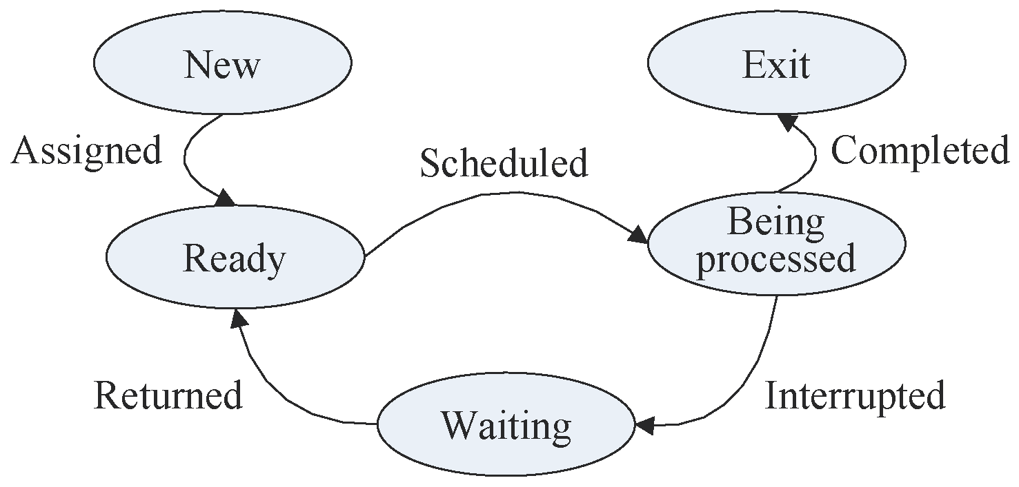
3.2. The Job State Transition

The job state transition is defined in Figure 2. There are five job states in total, corresponding to the five ellipses in the figure. The arrows and the text on the arrows indicate the state transition process of jobs. The five states are illustrated as follows.
New. If a job requests a human/robot, it will be created at first and wait for assignment;
Ready. If a new job is assigned to an idle human/robot, it is in a ready state; that is, a human/robot is occupied by the job and cannot be assigned to other jobs;
Being processed. If a ready job is scheduled, then it can start immediately. The job is in a being-processed state, and a human/robot is processing it;
Waiting. When a job is being processed, any interruption may break it off before its completion, and the interrupted job will be set as in a waiting state. If the interruption is completed in the waiting state, the job will be returned to the ready state;
Exit. Whenever a job is completed, it will exit the REI system, and the assigned human/robot will be released.

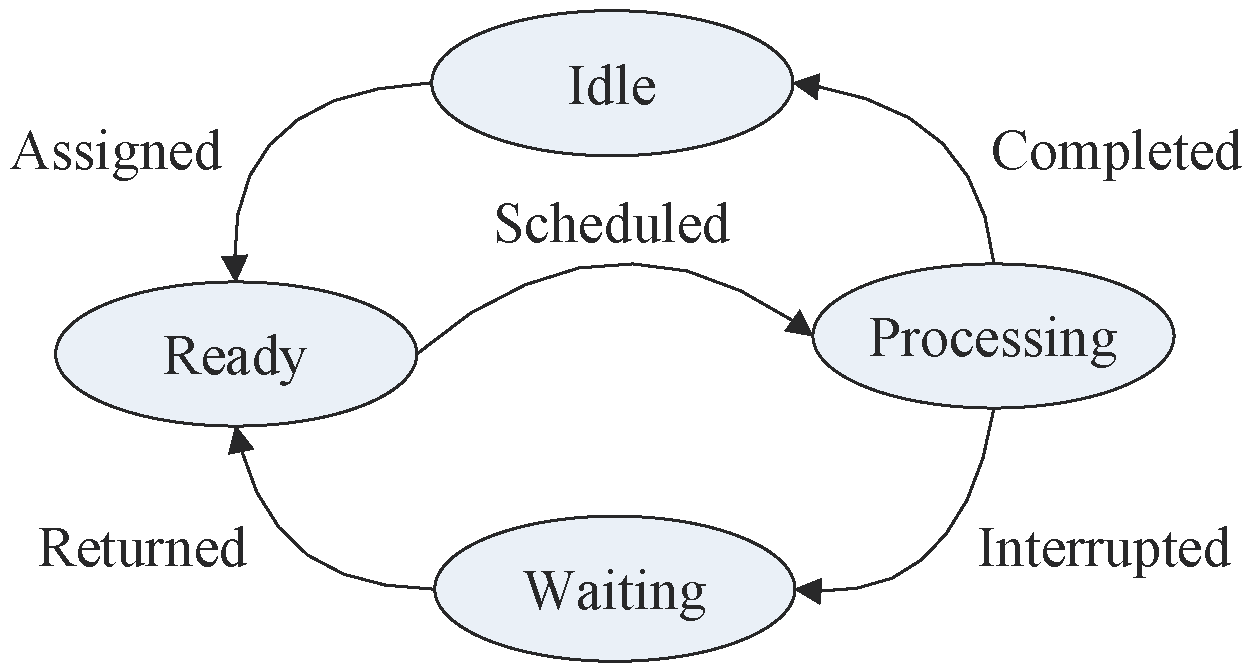
3.3. The Human/Robot State Transition

The human/robot state transition is shown in Figure 3. There are four human/robot states in total, corresponding to the four ellipses in the figure. The arrows and the text on the arrows indicate the state transition process of the human/robot. The four states are illustrated as follows.
Idle. This is an initial state, when a human/robot is not assigned to any jobs. Only an idle human/robot can be assigned to a job;
Ready. If an idle human/robot is assigned to a new job, it is in a ready state; that is, a human/robot is occupied by the job and cannot be assigned to other jobs;
Processing. If a ready human/robot is scheduled, then it can process the job immediately, and the job is in a being-processed state. Whenever the processing is completed, the human/robot will be idle again for the next assignments;
Waiting. When a human/robot is processing a job, any interruption may break it off before its completion, and the interrupted human/robot will be in a waiting state. If the interruption is completed in the waiting state, the human/robot will be returned to the ready state.

4. A Multi-Objective Model for EHCP

In this section, a multi-objective function is developed to both evaluate production performance and energy efficiency. The proposed model is more suitable for integrating and solving the two sub-problems, HSP and ESP.
Before defining a mathematical model for the problem, we make the following assumptions to simplify the analysis.
  • Assuming that the scheduling in human–machine collaboration is non-preemptive, without considering preemptive scheduling;
  • Assuming that different people can complete the same homework operation, regardless of the situation where someone is unable to perform a certain operation, including illness, emotions, and hunger;
  • Assuming that different robots can complete the same task operation, regardless of the situation where one robot is unable to perform a certain operation, such as faults, repairs, or power outages;
  • Assuming that the energy consumption of humans or robots is only related to their inherent power, without considering the increase or decrease in energy consumption rate under certain operations;
  • Assuming no special tasks applicable only to one person or one robot are considered.
In the energy-efficient human–robot collaboration problem, there is a set of jobs.
J = { J 1 , J 2 , , J j , , J j m a x }
The operation set of job j is given as
J j = { O j 1 , O j 2 , , O j o , , O j , o m a x }
The set of production lines is expressed as
P = { P 1 , P 2 , , P p , , P p m a x }
The set of humans and robots of production line P p is as follows
P p = { H p , R p }
The set of humans of production line P p is
H p = { H p 1 , H p 2 , , H p h , , H p , h m a x }
The set of robots of production line P p is presented as
R p = { R p 1 , R p 2 , , R p r , , R p , r m a x }
The job assignment on production line P p can be described as
J P p = { μ J 1 P p J 1 , μ J 2 P p J 2 , , μ J j P p J j , , μ J j m a x P p J j m a x }
The job assignment of job J j to human H p h can be defined as
J j H p h = { μ O j 1 H p h O j 1 , μ O j 2 H p h O j 2 , , μ O j o H p h O j o , , μ O j o m a x H p h O j , o m a x }
The job assignment of job J j to robot R p r can be expressed as
J j R p r = { μ O j 1 R p r O j 1 , μ O j 2 R p r O j 2 , , μ O j o R p r O j o , , μ O j o m a x R p r O j , o m a x }
The EHCP is an integration problem of two sub-problems, HSP and ESP, so its objective function includes two major parts: production performance and energy efficiency.

4.1. Production Performance of EHCP

Objective 1 is to minimize the makespan of all jobs, i.e., to minimize the maximum completion time, i.e., makespan.
m i n ( t Σ J j s p a n ) = m i n [ m a x ( t J j e n d ) ]
Subject to j j m a x , t J j e n d > 0 .
The optimal job assignment should ensure that each production line can obtain only one job at a time. If the makespan of the assigned jobs on all production lines is minimized, then objective 1 on the job layer can be obtained in each job assignment.
Objective 2 is to minimize the workload balance indicator λ .
m i n ( λ ) = p m a x p = 1 | L P p s u m L a v g |
Subject to
L P p s u m = j m a x j = 1 o m a x o = 1 [ h m a x h = 1 μ O j o H p h L H p h s u m + r m a x r = 1 μ O j o R p r L R p r s u m ] L P p m a x
L H p h s u m = o m a x o = 1 t H p h , O j o t o o l + t H p h , O j o s e t u p + t H p h , O j o m a c h + t H p h , O j o t r a n s L H p h m a x
L R p r s u m = o m a x o = 1 t R p r , O j o t o o l + t R p r , O j o s e t u p + t R p r , O j o m a c h + t R p r , O j o t r a n s L R p r m a x
p m a x p = 1 ( μ O j o H p h + μ O j o R p r ) = 1
In Equation (11), L P p s u m indicates the total workload of a production line P p , L a v g donates the average workload of all production lines, and | L P p s u m L a v g | denotes the divergence between the total workload L P p s u m of production line   P p and the average workload L a v g . Apparently, the λ is lower, and the workload balance between the different production lines is better.
Equation (12) is the constraint to be not greater than the maximum workload L P p m a x on production line P p , where the total workload L P p s u m of production line P p is represented as the sum of the total workload L H p h s u m on human H h , and the total workload L R p r s u m on robot R r in production line P p .
Equation (13) is the constraint to be not greater than the maximum workload L H p h m a x on human H h , where the total workload L H p h s u m on human H h is represented as the sum of the tool changing time t H p h , O j o t o o l , workpiece setup time t H p h , O j o s e t u p , machining time t H p h , O j o m a c h , and transportation time t H p h , O j o t r a n s of all operations assigned to human H h .
Equation (14) is the constraint to be not greater than the maximum workload L R p r m a x on robot R r , where the total workload L R p r s u m on robot R r is represented as the sum of the tool changing time t R p r , O j o t o o l , workpiece setup time t R p r , O j o s e t u p , machining time t R p r , O j o m a c h , and transportation time t R p r , O j o t r a n s of all operations assigned to robot R r .
Equation (15) describes that an operation O j o should be assigned to, at most, a human H p h or a robot R p r . If an operation O j o is processed on a robot or human H p h , then μ O j o H p h = 1 ; otherwise, μ O j o H p h = 0 .
Furthermore, the average workload of all production lines in Equation (11) can be calculated as the average of the sum of the total workload of each production line, as shown in Equation (16).
L a v g = 1 p m a x p m a x p L P p s u m
Objective 3 is to further minimize the makespan of all assigned operations on the production line P p .
m i n ( t Σ P p s p a n ) = m i n [ m a x ( t H p h , O j o e n d , t R p r , O j o e n d )   ]
S u b j e c t   t o : j j m a x , o o m a x , p p m a x , t H p h , O j o e n d > 0 ,   t R p r , O j o e n d > 0
Then, robotic edge intelligence can implement the operation assignment and assign each human H p h or each robot R p r to receive only one operation at a time. In each operation assignment, the robotic edge computing tries to minimize the makespan of assigned operations on all humans and robots to satisfy the requirements of objective 1 of the production line layer in Equation (10).
Objective 4 is to minimize the maximum workload of all production lines, where the humans and robots bear the most workload. The maximum workload of a production line P p can be calculated as
L P p m a x = max Pp ( h = 1 h m a x L H p h s u m + r = 1 r m a x L R p r s u m )
S u b j e c t   t o : L H p h s u m d i j / v H p h , L R p r s u m d i j / v R p r
In Equation (18), since L P p m a x represents the maximum workload of H p h and R p r , the value of L H p h s u m is considered the critical human workload on a human H p h , and the maximum value of L R p r m a x on robot R p r is considered the critical human workload. The constraint indicates that the workload L H p h s u m on human H h depends on the quotient of the travel distance d i j and human travel speed v H p h between two robots R i and R j , and the workload L R p r s u m on human R r depends on the quotient of the travel distance d i j and robot travel speed v R p r between two robots R i and R j .
Then, objective 4, to minimize the maximum total workload L P p m a x of all production lines, can be obtained by Equation (18).
L P p m a x = max Pp ( h = 1 h m a x L H p h s u m + r = 1 r m a x L R p r s u m )
S u b j e c t   t o : L H p h s u m L H p h m a x , L R p r s u m L R p r m a x

4.2. Energy Efficiency of EHCP

Then, the REI can further increase energy efficiency on the basis of the makespan in the former subsection. In the context of cleaner production, energy efficiency can be evaluated by the objectives as follows.
Subjective 5 is to minimize the total production energy consumption E P p s u m of all production lines. The production energy consumption of a production line P p includes human energy consumption and robot energy consumption, and each contains four parts: idle power, tool changing power, workpiece setup power, and machining power, as shown in Equations (18)–(20).
E P p s u m = h = 1 h m a x E H p h s u m + r = 1 r m a x E R p r s u m
E H p h s u m = t H p h i d l e P H p h i d l e + j m a x j = 1 o m a x o = 1 t H p h , O j o t o o l P H p h t o o l + t H p h , O j o s e t u p P H p h i d l e + t H p h , O j o m a c h P H p h m a c h + t H p h , O j o t r a n s P H p h t r a n s μ O j o H p h
E R p r s u m = t R p r i d l e P R p r i d l e + j m a x j = 1 o m a x o = 1 t R p r , O j o t o o l P R p r t o o l + t R p r , O j o s e t u p P R p r i d l e + t R p r , O j o m a c h P R p r m a c h + t R p r , O j o t r a n s P R p r t r a n s μ O j o R p r
Equation (20) indicates that the production energy consumption of production line P p includes human energy consumption in Equation (21) and robot energy consumption in Equation (22). In Equations (21) and (22), there are five parts, and each can be obtained by multiplying time and power, i.e., the idle energy consumption t H p h i d l e P H p h i d l e and t R p r i d l e P R p r i d l e , tool changing energy consumption t H p h , O j o t o o l P H p h t o o l and t R p r , O j o t o o l P R p r t o o l , workpiece setup energy consumption t H p h , O j o s e t u p P H p h i d l e and t R p r , O j o s e t u p P R p r i d l e , machining energy consumption t H p h , O j o m a c h P H p h m a c h and t R p r , O j o m a c h P R p r m a c h , and transportation energy consumption t H p h , O j o t r a n s P H p h t r a n s and t R p r , O j o t r a n s P R p r t r a n s .
Subjective 5 is to minimize the total production energy consumption E P p of all production lines based on Equations (20)–(22).
m i n ( E P p t o t a l ) = m i n p = 1 p m a x [ h = 1 h m a x E H p h s u m + r = 1 r m a x E R p r s u m ]
Objective 5 is subject to Equations (24) and (26).
t H p h , O j o e n d   m a x μ O j o 1 H p h t H p h , O j o 1 e n d , μ O j o 1 R p r t R p r , O j o 1 e n d + μ O j o H p h t H p h , O j o t o o l + t H p h , O j o s e t u p + t H p h , O j o m a c h
t R p r , O j o e n d   m a x μ O j o 1 H p h t H p h , O j o 1 e n d , μ O j o 1 R p r t R p r , O j o 1 e n d + μ O j o R p r t R p r , O j o t o o l + t R p r , O j o s e t u p + t R p r , O j o m a c h + t R p r , O j o t r a n s
t O j o e n d t O j o 1 e n d m a x [ μ O j o H p h t H p h , O j o t o o l + t H p h , O j o s e t u p + t H p h , O j o m a c h , μ O j o R p r t R p r , O j o t o o l + t R p r , O j o s e t u p + t R p r , O j o m a c h + t R p r , O j o t r a n s ]
Equation (24) restricts that the completion time of the current operation O j o on a human H p h cannot be processed before the completion of the former operation O j ( o 1 ) on the same human H p h or a robot R p r . Additionally, the completion time of the current operation O j o should consider the tool changing time, workpiece setup time, and machining time of a human H p h .
Equation (25) checks that the completion time of the current operation O j o on a robot R p r cannot be processed before the completion of the former operation O j ( o 1 ) on the same robot R p r or a human H p h . In addition, the completion time of the current operation O j o should consider the tool changing time, workpiece setup time, machining time, and transportation time of a robot R p r .
Equation (26) confines that the current operation O j o cannot be processed before the completion of the former operation O j ( o 1 ) on a human or a robot.
Therefore, the energy-efficient human–robot collaboration problem can be described as a nonlinear multi-objective function, as shown in Equation (27).
O b j = min t Σ J j s p a n , min λ , m i n ( t Σ P p s p a n , m i n ( L P p m a x ) , m i n ( E P p t o t a l ) }
Subjective to Equations (1)–(26).
The multi-objective function in Equation (27) considers the minimization of the makespan of all assigned jobs t Σ J j s p a n , workload balance indicator λ , the makespan of all assigned operations on the production line t Σ P p s p a n , the maximum human/robot workload L P p m a x of production lines, and the production energy consumption E P p of production lines. The multi-objective function has several conflicting objectives and nonlinear constraints, and it is not easy for traditional algorithms to search for the optimal solutions. The next section introduces a heuristic search algorithm to address the challenge.

5. An Artificial Plant Community Algorithm

In this section, an artificial plant community algorithm [30] is designed and developed to solve the energy-efficient human–robot collaboration problem and balance production performance and energy efficiency. The APC algorithm is very simple and requires very little hardware, so it can run on multiple edge robots to form powerful swarm intelligence.

5.1. Solution Steps of APC

The solution steps of an artificial plant community are introduced in detail, which has five main steps, i.e., initialization, seeding, growing, fruiting, and end judgment. An artificial plant individual has three forms, i.e., a seed, an individual, and a fruit.

5.1.1. Step 1: Initialization

In this step, the main parameters will be initialized for the EHCP, the APC, and the solving system.
The parameters of EHCP are composed of the set of jobs J = { J j } , the operation set of job J j = { O j o } , the set of production lines P = { P p } , the set of humans H p = { H p h } and robots R p = { R p r } of a production line P p , the maximum human/robot workload L P p m a x , the maximum workload L H p h m a x of a human, the maximum workload L R p r m a x of a robot, the idle power P H p h i d l e of a human, the idle power P R p r i d l e of a robot, the tool changing power P H p h t o o l of a human, the tool changing power P R p r t o o l of a robot, the machining power P H p h m a c h of a human, the machining power P R p r m a c h of a robot, the transportation power P H p h t r a n s of a human, and the transportation power P R p r t r a n s of a robot.
The parameters of APC involve the population size S , seeding probability p s e e d , growing probability p g r o w , fruiting probability p f r u i t , and artificial plant individual x i . Therefore, an artificial plant community can be defined as a job shop assignment set X = { x 1 , x 2 , , x i , , x S } . The multi-objective function O b j in Equation (27) can be selected to construct a fitness function f i t of APC.
f i t = C O b j
where C is a positive constant enough large. Therefore, the larger the fitness f i t is, the better the solution is.
The parameters of the solving system contain the maximum number of iterations I t e m a x , iteration counter I t e , the error threshold e t h , and the maximum solving period T .

5.1.2. Step 2: Seeding of APC

The seeding operation is a global search process where the seeds x i produced during the first seeding are different from those produced during subsequent seeding.
x i = { μ O j o H p h , μ O j o R p r }
The first seeding takes place after initialization. In the first iteration, the artificial plant community will be randomly generated in all edge robots to search for feasible solutions, and the initial seeds will be fully random with a population size S . Therefore, the solution of the APC algorithm is independent of the initial state of the feasible solutions or seeds.
The following seeding operations take place in subsequent iterations, where the fruits produced in the previous fruiting operations with a population size S will be selected as the seeds, and a part of random seeds are generated at the same time with a population size of p s e e d × S . The best fruits with a population size S in the previous iteration and the random seeds with a population size of p s e e d × S constitute a new generation of seeds with a population size of ( 1 + p s e e d ) × S .
The smaller the seeding probability p s e e d is, the lower the global search capability is, but the faster the convergence is, and this may even lead to a premature convergence to the local optima. On the contrary, the greater the seeding probability p s e e d is, the greater the global search capability is, but the slower the convergence is.

5.1.3. Step 3: Growing of the APC

The growing operation is a natural selection process where not all artificial plant seeds can survive after the seeding operation, so the population size of APC will reduce after the growing operation.
After the growing operation, the population size of APC decreases to p g r o w × S , while the rest of the population ( 1 p g r o w ) × S dies. According to the fitness function f i t in Equation (28), the elite solutions in the growing stage can be described as x i in Equation (28).
x i = { x i | f i t x i p g r o w S f i t ( x i ( 1 p g r o w ) S ) }
The greater the growing probability p g r o w is, the lower the global search capability is, but the faster the convergence is, and this may even lead to a premature convergence to the local optima. On the contrary, the smaller the growing probability p g r o w is, the greater the global search capability is, but the slower the convergence is.
The APC individual with the highest fitness levels is the most important elite solution in the search process.
x i # = { x i # | f i t x i # = m a x [ f i t x i ] }
Here, a group sort is employed to help us implement quick selection. The group sort first randomly divides the seeds into p g r o w × S groups, and each group has two or three seeds. Then, each group selects the best seed to grow, where there are only one or two comparisons in each group. Therefore, the group sort has a time performance of O ( S ) and space performance of O ( S ) to obtain the best solution.

5.1.4. Step 4: Fruiting of the APC

In the fruiting operation, this part of the surviving elite individuals will socially learn to generate more individuals, i.e., fruits. Now, the APC population has recovered to its original size. The fruiting operation can be realized by binary and/or/not operations on robotic embed platforms.
The first fruit comes from the APC individual x i # with the highest fitness, which can produce a fully identical fruit through parthenogenesis.
x i ( t ) = x i # ( t 1 )
The other fruits come from social learning between different individuals. The fruiting probability p f r u i t decides how much information is kept from the parent individuals for the new generation of fruits. Therefore, a parent individual can learn a portion of information from other plant individuals by probability ( 1 p f r u i t ) .

5.1.5. Step 5: End Judgment

The end condition can be justified by the maximum number of iterations I t e m a x , the error threshold e t h , or the maximum solving period T .

5.2. Pseudo-Codes of APC

According to the algorithm steps above, the corresponding pseudo-codes are shown in Algorithm 1, where the APC individual is encoded by Equation (27), and the objective function in Equation (25) is selected for fitness calculation and comparison. The state transition of jobs, humans, and robots is referred to in Figure 2 and Figure 3.
Algorithm 1: Solving EHCP in the job layer
1:initialize the parameters of EHCP
2:initialize the parameters of APC
3:initialize the parameters of the solving system
4:if state (job) = new
5:if state (human) = idle
6:if state (robot) = idle
7:encode the APC individual by Equation (29)
8:select objectives 2 and 3 by Equation (27)
9:for ite: 1 to I t e m a x
10:generate the random seeds by p s e e d
11:generate seeds from the previous fruits
12:calculate and compare fitness by Equation (27)
13:select the best solutions by p g r o w
14:select the elite individual with the highest fitness
15:generate a best fruit through parthenogenesis
16:generate fruits through social learning by p f r u i t
17:end judgment by e t h
18:end for
19:output the optimal solution
20:State (job) = ready
21:State (human) = ready
22:State (robot) = ready
Then, the optimal solution to the EHCP will be output to assign jobs to humans or robots. The states of jobs, humans, and robots will be updated as a ready state.

6. Benchmark Experiments

This section provides a benchmark data set and conducts a series of benchmark experiments to test the proposed method for solving the energy-efficient human–robot collaboration problem.

6.1. Benchmark Data

The benchmark data set is based on references [2,10] in real-world data, and necessary adjustments have been made to meet our testing objectives and requirements.
Figure 4 shows the roadmap of a benchmark workpiece. There are fifteen humans H = { H 1 , H 2 , , H 15 } and fifteen robots R = { R 1 , R 2 , , R 15 }. Each robot has a 7.5 m interval between them. According to the benchmark roadmap in Figure 4, the travel distances d i j between consecutive robots R i and R j are shown in Table 1. These data have been simplified to facilitate benchmarking by international peers. The first robot R 1 is assumed as the start node, and all jobs are on robot R 1 from the beginning. The human–robot collaboration continues until the final job is completed.
The workload L R p r on robots for fifteen operations O = O 1 , O 2 , , O 15 is provided in Table 2. The workloads are in the range of [5, 30] min, so the benchmark data are consistent with real-world scenarios [2,10]. Then, the energy consumption of robots can be calculated by multiplying the workload L R p r and the robot power P R p r .
The idle power P R p r i d l e consumed by the robots is shown in the second line in Table 3, within the range of [30, 120], and the setup power is the same. The processing power P R p r m a c h for each robot is provided in the third line in Table 3 within the range of [150, 500], and the transportation power P R p r t r a n s is the same. They come from a set of robots in real-world data. Then, the idle energy consumption can be calculated by multiplying the idle time and the idle power P R p r i d l e , and the idle time can be calculated by subtracting the workload from the total working time of the robot. Hence, the total energy consumption E R p r s u m can be calculated by adding the processing energy consumption and the idle energy consumption, as shown in Equation (22).
Since these benchmark data are derived and modified from the existing literature and data in real-world workpiece systems [2,10], they are reasonable and suitable for our test objectives.

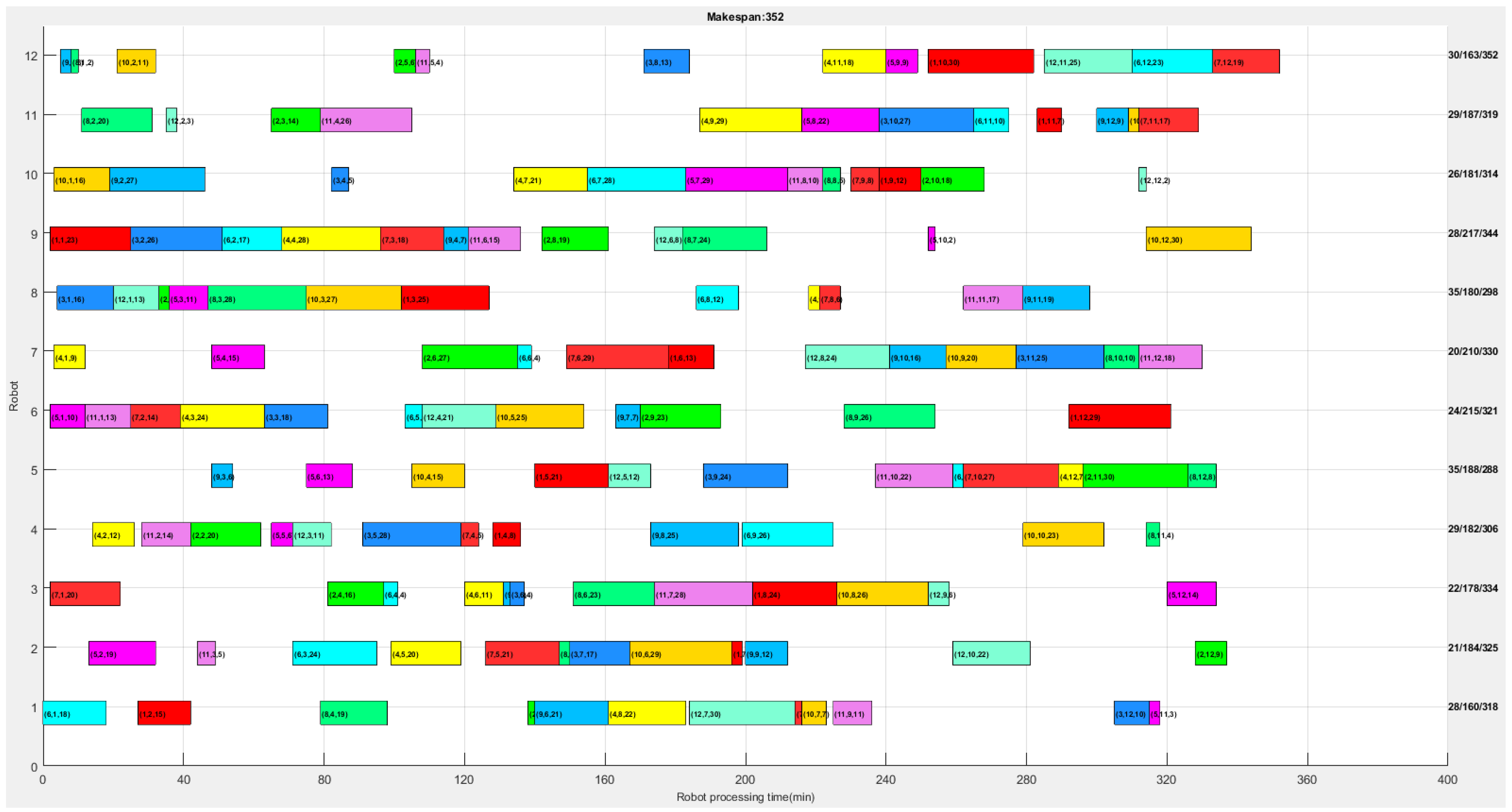
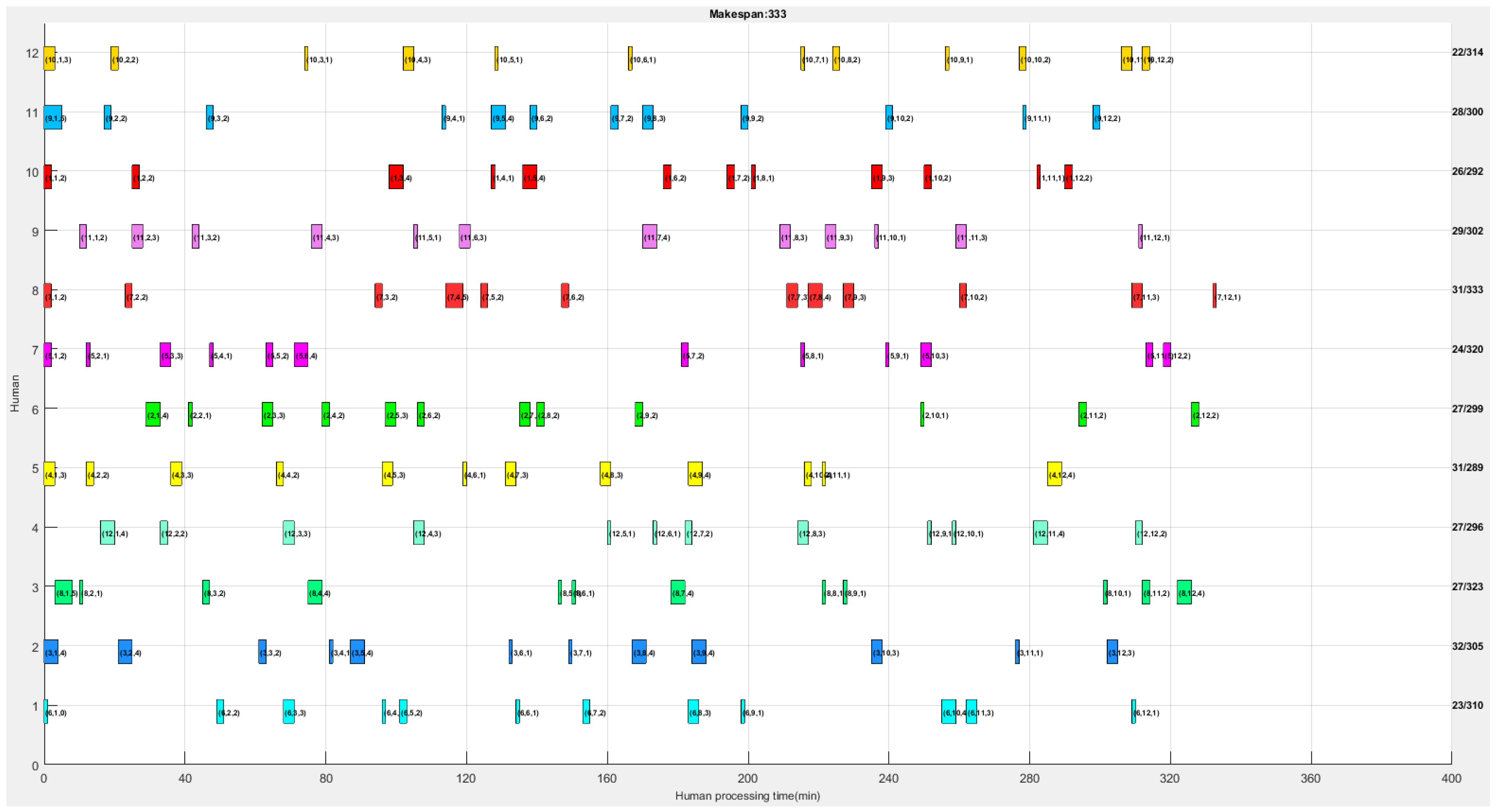
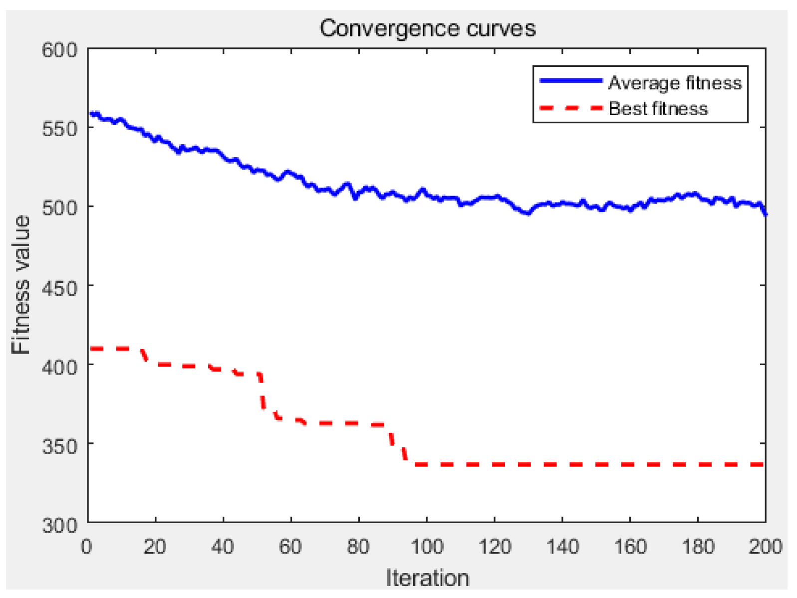
6.2. Experimental Results

This section presents our experimental results of the benchmark data above. Our experimental platform has an AMD Ryzen 3 4300U with Radeon Graphics 2.70 GHz CPU, 8.00 GB RAM, 64-bit Windows 10 operating system, and MATLAB R2018a simulation software. The objective function in Equation (27) is employed to test the benchmark data, including the total makespan t Σ J j s p a n in Equation (10), workload balance indicator λ in Equation (11), human energy consumption E H p h s u m in Equation (21), and robot energy consumption E R p r s u m in Equation (22). The parameters of the APC algorithm set the population size = 100, the seeding probability p s = 0.2 , the growing probability p g = 0.7 , and the fruiting possibility p f = 0.1 . The maximum number of iterations I t e m a x = 200 , and the maximum computation time for termination = 0.5 h.
The processing time of robots is shown in the Gantt chart of Figure 5, and the makespan value t Σ J j s p a n = 352 min is labeled at the top of Figure 5. The vertical axis indicates the robot number, the horizontal axis indicates the robot workload in minutes, and the right side gives the human workload L H p h s u m , the robot workload L R p r s u m , and the maximum completion time of each robot in fractional form, respectively. Each progress bar is marked by three numbers enclosed in parentheses to show the job number J j , operation number O j o , and workload L R p r , respectively. The different colors indicate different jobs and operations. Figure 5 represents the example of the minimum makespan, and the processing energy consumption of robots can be obtained by multiplying the workload L R p r s u m and the processing power P R p r m a c h in Table 3 to be 10.596 kWh. Since the rest time is idle time, the idle energy consumption of robots can be obtained by multiplying the idle time t R p r i d l e and the idle power P R p r i d l e in Table 3 to be 2.026 kWh. Hence, the total energy consumption E R p r s u m of all robots can be calculated at 12.622 kWh.
The processing time of humans is presented in the Gantt chart of Figure 6, and the human makespan value of 333 min is labeled at the top of Figure 6. The vertical axis indicates the human number, the horizontal axis indicates the human workload in minutes, and the right side gives the human workload L H p h s u m and the maximum completion time of each human in fractional form, respectively. Each progress bar is marked by three numbers enclosed in parentheses to show the job number J j , operation number O j o , and workload L H p h , respectively. The different colors indicate different jobs and operations. We do not consider human energy consumption here, only the energy consumption of robots. The human workload L H p h s u m and the maximum idle time t H p h i d l e can be obtained as 324 min and 302 min, respectively.
The convergence curves of the Gantt charts in Figure 5 and Figure 6 are shown in Figure 7, and the proposed method obtains the optimal solution after about 94 iterations with a maximum iteration of 200. It verifies that the proposed method has both good global search ability and fast convergence ability.
Table 4 shows the statistics of the artificial plant community algorithm on the benchmark test in 300 time experiments, including the makespan t Σ J j s p a n of all jobs in Equation (10), the workload balance indicator λ in Equation (11), the makespan on the production line P p in Equation (17), the maximum workload L P p m a x of all production lines in Equation (18), the total energy consumption E R p r s u m of all robots in Equation (22), the total workload L H p h s u m of humans in Equation (13), etc. As can be seen, the minimum value of makespan t Σ J j s p a n has a 13.30% improvement compared to the maximum value, and t Σ P p s p a n has a 13.30% improvement. At the same time, the workload balance indicator λ has a 25.81% improvement compared to the maximum value, and the maximum human/robot workload L P p m a x has a 2.39% improvement. The total energy consumption E R p r s u m of all robots has a 4.88% improvement compared to the maximum value, and the total workload L H p h s u m of humans has a 5.81% improvement. These verify that the proposed method is efficient in solving the energy-efficient human–robot collaboration problem.
Figure 8 presents the trend of four main metrics with different human/robot numbers, and their values were normalized due to the different dimensions of the four metrics. It can be seen from Figure 8a that more humans can greatly reduce the minimum makespan t Σ J j s p a n and robot energy consumption E R p r s u m , but with greater human workload L H p h s u m . Figure 8b shows that more robots can greatly improve production efficiency and reduce the minimum makespan t Σ J j s p a n , but with greater robot energy consumption E R p r s u m and more human workload L H p h s u m . If we want to balance the four metrics, four humans and six robots seem to be appropriate when the makespan curve intersects exactly with the human workload curve in Figure 8a,b, respectively.
Here are some suggestions for the EHCP in engineering applications. First, production efficiency and production cost often conflict. Higher production efficiency and lower makespan t Σ J j s p a n require more human workload L H p h s u m and robot energy consumption E R p r s u m . Second, human workload L H p h s u m and robot energy consumption E R p r s u m are a pair of contradictions. More human workload L H p h s u m is helpful to reduce robot energy consumption E R p r s u m , and vice versa. Third, production efficiency t Σ J j s p a n and the workload balance indicator λ are both contradictory and unified. Fourth, the appropriate number of humans and robots is helpful to balance the five metrics, i.e., four humans and six robots.

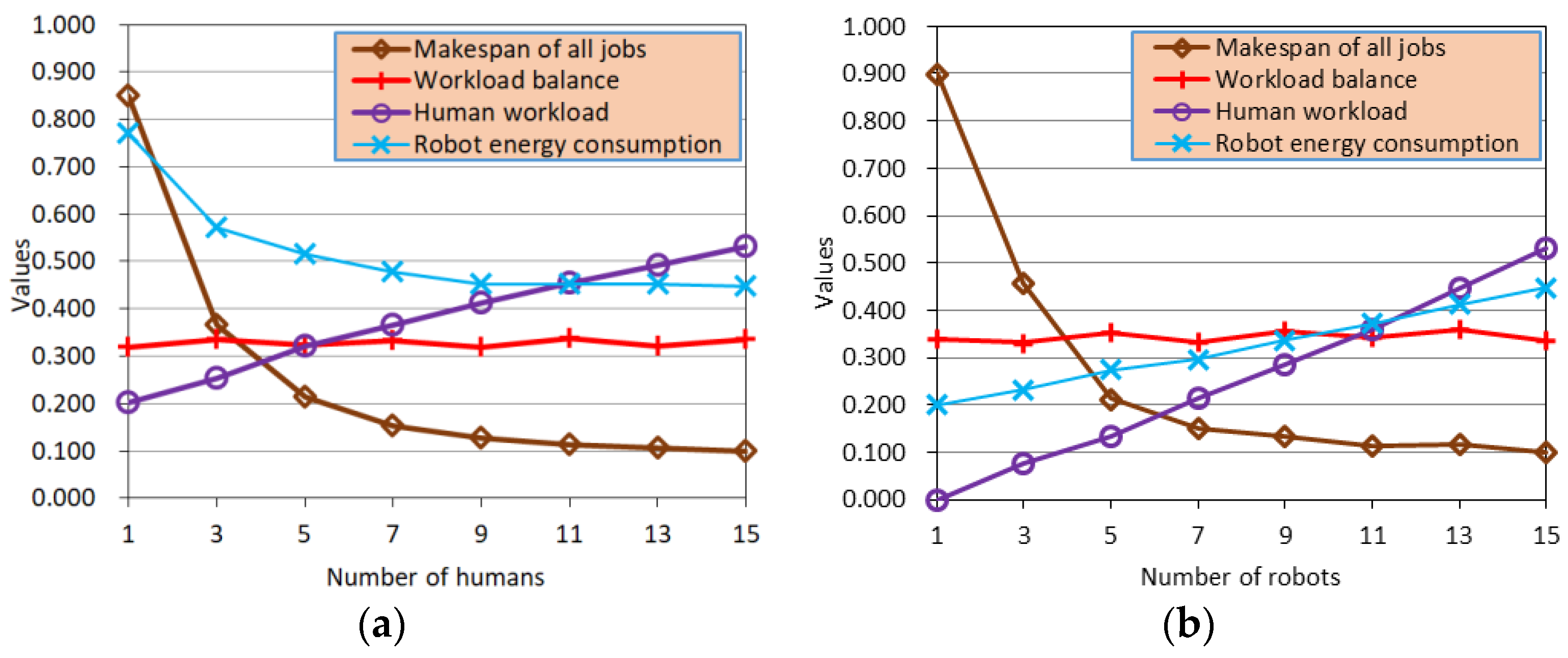
6.3. Comparative Analysis

In this section, the comparison results of EHCP for each method are shown in Table 5, including GA [1,6,12,23], ACO [11], ABC [13], PSO [14], QL [25], and the proposed APC. The first column lists three important indicators, including the makespan t Σ J j s p a n of all jobs, the workload balance indicator λ , the makespan on the production line P p , the maximum workload L P p m a x of all production lines, the total energy consumption E R p r s u m of all robots, the total workload L H p h s u m of humans, and the solution time. The results of each algorithm include two groups of data, i.e., the minimum values (min in Table 5) and the average (avg in Table 5) values. They are obtained after 50 runs.
As we can see from Table 5, the proposed APC algorithm obtains a minimum makespan t Σ J j s p a n of 352 min and an average makespan t Σ J j s p a n of 371.333 min. Therefore, the proposed APC algorithm can improve the minimum makespan to 1.124% and the average makespan to 1.772% compared to the maximum compartments, respectively. The proposed APC algorithm has a minimum workload balance indicator λ of 30.667 min and an average value of 36.667 min. Hence, the proposed APC algorithm can improve the minimum workload balance indicator λ to 4.664% and the average value to 4.347%, respectively.
As the total energy consumption E R p r s u m of all robots, the best minimum value and average value in the compared algorithms are 12.622 kWh and 12.955 kWh, respectively. Therefore, the proposed APC algorithm can improve the minimum robot energy consumption E R p r s u m to 2.242% and the average value to 2.203% compared to the maximum values. As the total workload L H p h s u m of humans, the best minimum value and average value in the compared algorithms are 324 min and 334.133 min, respectively. Hence, the proposed APC algorithm can improve the minimum human workload L H p h s u m to 1.210% and the average value to 1.213%, respectively.
To sum up, the scheduling results of EHCP in our proposed method have advantages over the STOA algorithms in minimum values and average values, and it is easier to search for the global optimal solutions in a short solution time. In our testing, the initial parameters of APC may be the optimal configuration. In engineering applications, balancing production performance (such as minimizing completion time) and energy efficiency is extremely challenging. In some emergency situations, optimizing production performance is more urgent, but it may lead to suboptimal results in energy efficiency or vice versa. However, adjusting the multi-objective function of this model can assist engineering and management personnel in balancing these conflicting objectives and making them more in line with actual production needs.

7. Conclusions and Future Directions

Today, more and more enterprises apply all kinds of robots to improve production performance, but robots are also very energy-consuming. The energy-efficient human–robot collaboration affects the sustainability of production systems and the environment. Optimizing energy-efficient human–robot collaboration is a great challenge to traditional cloud centers and production systems. Our work provides a robotic edge intelligence architecture to address it. Our work has four main contributions. Firstly, an REI architecture is built, and a series of edge robots are utilized to solve the EHCP, which provides a novel insight into the theoretical and practical application of robotic edge intelligence. Secondly, a multi-objective function is designed to instruct the edge robots to optimize the job assignment and enhance both production performance and energy efficiency. Thirdly, a novel artificial plant community algorithm is proposed to solve the EHCP, which has low requirements for hardware and can be easily deployed in edge robots for distributed computing. Fourthly, a benchmark data set is developed, and a series of benchmark experiments are conducted.
Our shortcomings and future research include at least three parts. First, a real human–robot collaboration system may be more complex, and the long-term sustainability impacts of the proposed system beyond immediate energy efficiency and production performance should be surveyed and considered. Determining the optimal configuration is a highly challenging task, which is related to the type, scale, and scenario of the problem to be solved. Second, more edge computing technologies should be integrated with real human–robot collaboration systems. A lifecycle analysis is necessary to assess the environmental impact of implementing the robotic edge intelligence system. Third, more benchmark data are required to test the proposed algorithm and compare more SOTA methods, such as simulated annealing.

Author Contributions

Conceptualization, Z.C. (Zhengying Cai) and X.D.; methodology, Z.C. (Zhengying Cai), X.D. and T.H.; validation, T.L., Z.C. (Zhiheng Cai), and G.G.; writing—original draft preparation, Z.C. (Zhengying Cai) and X.D.; writing—review and editing, X.D., T.H., T.L. and Z.C. (Zhiheng Cai); supervision, Z.C. (Zhengying Cai) and G.G.; project administration, Z.C. (Zhengying Cai) and G.G.; funding acquisition, Z.C. (Zhengying Cai). All authors have read and agreed to the published version of the manuscript.

Funding

This research was funded by the National Natural Science Foundation of China (no. 71471102), Major Science and Technology Projects in Hubei Province of China (grant no. 2020AEA012), and Yichang University Applied Basic Research Project in China (grant no. A17-302-a13).

Institutional Review Board Statement

The study did not require ethical approval.

Informed Consent Statement

Not applicable.

Data Availability Statement

Data are contained within the article.

Acknowledgments

The authors thank the hard work of all anonymous reviewers to improve the quality of this submission.

Conflicts of Interest

The authors declare no conflicts of interest.

References

  1. Mura, M.D.; Dini, G. Job rotation and human-robot collaboration for enhancing ergonomics in assembly lines by a genetic algorithm. Int. J. Adv. Manuf. Technol. 2022, 118, 2901–2914. [Google Scholar] [CrossRef]
  2. Lu, C.; Gao, R.; Yin, L.; Zhang, B. Human–robot collaborative scheduling in energy-efficient welding shop. IEEE Trans. Ind. Inform. 2024, 20, 963–971. [Google Scholar] [CrossRef]
  3. Guo, D. Fast scheduling of human-robot teams collaboration on synchronised production-logistics tasks in aircraft assembly. Robot. Comput. Manuf. 2024, 85, 102620. [Google Scholar] [CrossRef]
  4. Subramanian, K.; Thomas, L.; Sahin, M.; Sahin, F. Supporting human–robot interaction in manufacturing with augmented Reality and effective human–computer interaction: A review and framework. Machines 2024, 12, 706. [Google Scholar] [CrossRef]
  5. Zhang, R.; Lv, Q.; Li, J.; Bao, J.; Liu, T.; Liu, S. A reinforcement learning method for human-robot collaboration in assembly tasks. Robot. Robot. Comput. Integr. Manuf. 2022, 73, 102227. [Google Scholar] [CrossRef]
  6. Mura, M.D.; Dini, G. Designing assembly lines with humans and collaborative robots: A genetic approach. CIRP Nals-Manuf. Technol. 2019, 68, 1–4. [Google Scholar] [CrossRef]
  7. Qu, C.; Sorbelli, F.B.; Singh, R.; Calyam, P.; Das, S.K. Environmentally-aware and energy-efficient multi-drone coordination and networking for disaster response. IEEE Trans. Netw. Serv. Manag. 2022, 20, 1093–1109. [Google Scholar] [CrossRef]
  8. Gao, Z.G.; Yang, R.N.; Zhao, K.; Yu, W.H.; Liu, Z.; Liu, L.L. Hybrid convolutional neural network approaches for recognizing col-laborative actions in human-robot assembly tasks. Sustainability 2024, 16, 139. [Google Scholar] [CrossRef]
  9. Lachner, J.; Allmendinger, F.; Hobert, E.; Hogan, N.; Stramigioli, S. Energy budgets for coordinate invariant robot control in physical human–robot interaction. Int. J. Robot. Res. 2021, 40, 968–985. [Google Scholar] [CrossRef]
  10. Alevizos, K.I.; Bechlioulis, C.P.; Kyriakopoulos, K.J. Bounded energy collisions in human–robot cooperative transportation. IEEE/ASME Trans. Mechatron. 2022, 27, 4541–4549. [Google Scholar] [CrossRef]
  11. Elmi, A.; Topaloglu, S. Cyclic job shop robotic cell scheduling problem: Ant colony optimization. Comput. Ind. Eng. 2017, 111, 417–432. [Google Scholar] [CrossRef]
  12. Wu, T.; Zhang, Z.; Zeng, Y.; Zhang, Y. Mixed-integer programming model and hybrid local search genetic algorithm for human–robot collaborative disassembly line balancing problem. Int. J. Prod. Res. 2023, 62, 1758–1782. [Google Scholar] [CrossRef]
  13. Huang, Y.; Sheng, B.; Luo, R.; Lu, Y.; Fu, G.; Yin, X. Solving human-robot collaborative mixed-model two-sided assembly line balancing using multi-objective discrete artificial bee colony algorithm. Comput. Ind. Eng. 2024, 187, 109776. [Google Scholar] [CrossRef]
  14. Omidi, M.; Van de Perre, G.; Hota, R.K.; Cao, H.-L.; Saldien, J.; Vanderborght, B.; El Makrini, I. Improving postural ergonomics during human–robot collaboration using particle swarm optimization: A study in virtual environment. Appl. Sci. 2023, 13, 5385. [Google Scholar] [CrossRef]
  15. Khosravy, M.; Gupta, N.; Pasquali, A.; Dey, N.; Crespo, R.G.; Witkowski, O. Human-collaborative artificial intelligence along with social values in industry 5.0: A survey of the state-of-the-art. IEEE Trans. Cogn. Dev. Syst. 2024, 16, 165–176. [Google Scholar] [CrossRef]
  16. Cai, Z.; Wang, X.; Li, R.; Gao, Q. An artificial physarum polycephalum colony for the electric location-routing problem. Sustainability 2023, 15, 16196. [Google Scholar] [CrossRef]
  17. Cai, Z.; Li, G.; Zhang, J.; Xiong, S. Using an artificial physarum polycephalum colony for threshold image segmentation. Appl. Sci. 2023, 13, 11976. [Google Scholar] [CrossRef]
  18. Chen, Y.; Li, Y.S. Storage location assignment for improving human-robot collaborative order-picking efficiency in robotic mobile fulfillment systems. Sustainability 2024, 16, 1742. [Google Scholar] [CrossRef]
  19. Lyu, S.; Cheah, C.C. Human-robot interaction control based on a general energy shaping method. IEEE Trans. Control Syst. Technol. 2020, 28, 2445–2460. [Google Scholar] [CrossRef]
  20. Aydogan, Ç.; Gürel, S. Energy efficient scheduling of a two machine robotic cell producing multiple part types. Flex. Serv. Manuf. J. 2024, 1–35. [Google Scholar] [CrossRef]
  21. Ye, X.; Deng, Z.; Shi, Y.; Shen, W. Toward Energy-Efficient Routing of Multiple AGVs with Multi-Agent Reinforcement Learning. Sensors 2023, 23, 5615. [Google Scholar] [CrossRef] [PubMed]
  22. Chen, X.L.; Du, Y. Hybrid artificial immune algorithm for energy-efficient distributed flexible job shop in semiconductor manufacturing. Clust. Comput. J. Netw. Softw. Tools Appl. 2023, 27, 3075–3098. [Google Scholar] [CrossRef]
  23. Wei, H.; Li, S.; Quan, H.; Liu, D.; Rao, S.; Li, C.; Hu, J. Unified multi-objective genetic algorithm for energy efficient job shop scheduling. IEEE Access 2021, 9, 54542–54557. [Google Scholar] [CrossRef]
  24. Luo, S.; Zhang, L.; Fan, Y. Energy-efficient scheduling for multi-objective flexible job shops with variable processing speeds by grey wolf optimization. J. Clean. Prod. 2019, 234, 1365–1384. [Google Scholar] [CrossRef]
  25. Zhao, F.; Di, S.; Wang, L. A hyperheuristic with Q-learning for the multiobjective energy-efficient distributed blocking flow shop scheduling problem. IEEE Trans. Cybern. 2022, 53, 3337–3350. [Google Scholar] [CrossRef]
  26. Wang, G.; Li, X.; Gao, L.; Li, P. An effective multi-objective whale swarm algorithm for energy-efficient scheduling of distributed welding flow shop. Ann. Oper. Res. 2022, 310, 223–255. [Google Scholar] [CrossRef]
  27. Tirkolaee, E.B.; Goli, A.; Weber, G.-W. Fuzzy mathematical programming and self-adaptive artificial fish swarm algorithm for just-in-time energy-aware flow shop scheduling problem with outsourcing option. IEEE Trans. Fuzzy Syst. 2020, 28, 2772–2783. [Google Scholar] [CrossRef]
  28. Wu, M.; Yeong, C.F.; Su, E.L.M.; Holderbaum, W.; Yang, C. A review on energy efficiency in autonomous mobile robots. Robot. Intell. Autom. 2023, 43, 648–668. [Google Scholar] [CrossRef]
  29. Czymmek, V.; Köhn, C.; Harders, L.O.; Hussmann, S. Review of energy-efficient embedded system acceleration of convolution neural networks for organic weeding robots. Agriculture 2023, 13, 2103. [Google Scholar] [CrossRef]
  30. Cai, Z.; Jiang, S.; Dong, J.; Tang, S. An artificial plant community algorithm for the accurate range-free positioning of wireless sensor networks. Sensors 2023, 23, 2804. [Google Scholar] [CrossRef]
  31. Katare, D.; Perino, D.; Nurmi, J.; Warnier, M.; Janssen, M.; Ding, A.Y. A survey on approximate edge AI for energy efficient au-tonomous driving services. IEEE Commun. Surv. Tutor. 2023, 25, 2714–2754. [Google Scholar] [CrossRef]
  32. Liu, H.H.; Nasiriany, S.; Zhang, L.C.; Bao, Z.Y.; Zhu, Y.K. Robot learning on the job: Human-in-the-loop autonomy and learning during deployment. arXiv 2024, arXiv:2211.08416. [Google Scholar] [CrossRef]
  33. Cao, Y.; Zhou, Q.; Yuan, W.; Ye, Q.; Popa, D.; Zhang, Y. Human-robot collaborative assembly and welding: A review and analysis of the state of the art. J. Manuf. Process. 2024, 131, 1388–1403. [Google Scholar] [CrossRef]
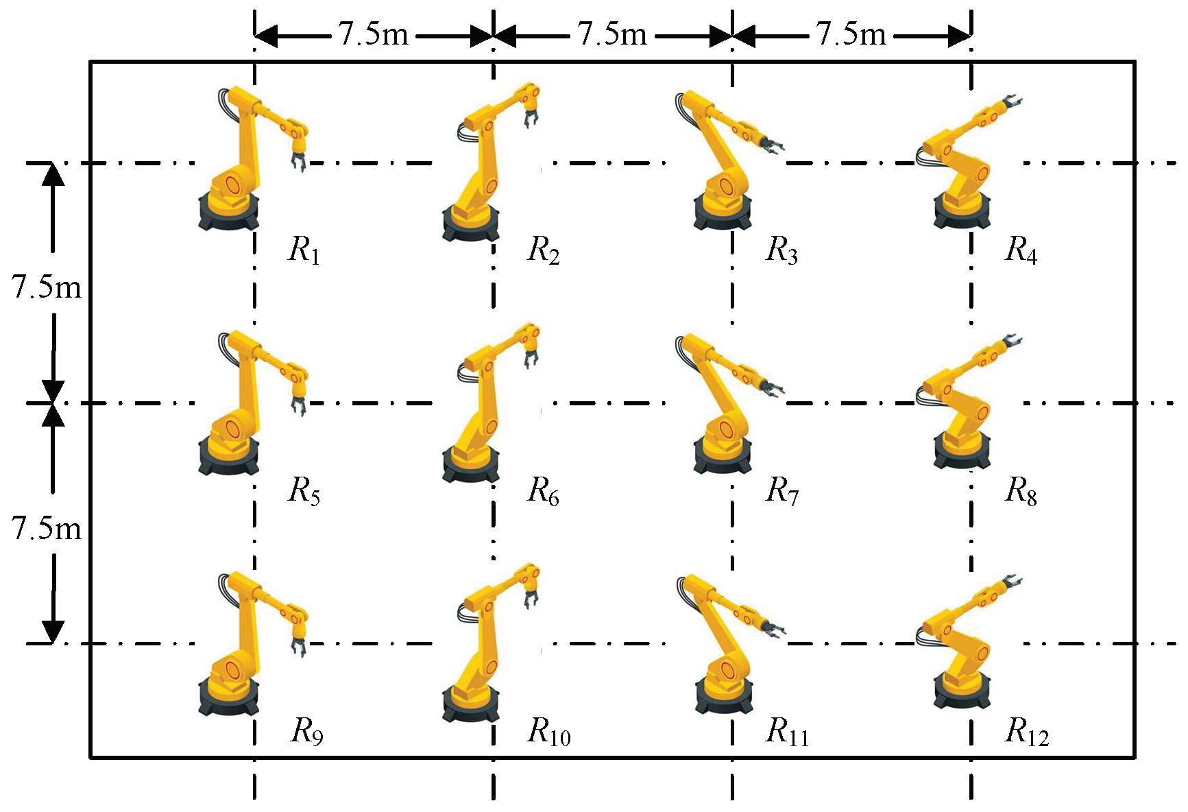
Figure 1. An REI architecture for modern production systems.
Sustainability 16 09788 g001
Figure 2. The job state transition.
Sustainability 16 09788 g002
Figure 3. The human/robot state transition.
Sustainability 16 09788 g003
Figure 4. Benchmark roadmap in a workpiece.
Sustainability 16 09788 g004
Figure 5. The processing time for robots. (The same color is used for different processes of the same job, and different colors are randomly assigned to different jobs).
Sustainability 16 09788 g005
Figure 6. The processing time for humans. (The same color is used for different processes of the same job, and different colors are randomly assigned to different jobs.)
Sustainability 16 09788 g006
Figure 7. The convergence curves of the proposed method.
Sustainability 16 09788 g007
Figure 8. Comparison of parameter changes. ((a) is the trend of five main metrics with different human numbers, (b) is the trend of five main metrics with different robot numbers).
Sustainability 16 09788 g008
Table 1. The travel distance (m) between consecutive robots.
Robots R 1 R 2 R 3 R 4 R 5 R 6 R 7 R 8 R 9 R 10 R 11 R 12
R 1 07.51522.57.51522.5301522.53037.5
R 2 7.507.515157.51522.522.51522.530
R 3 157.507.522.5157.5153022.51522.5
R 4 22.5157.503022.5157.537.53022.515
R 5 7.51522.53007.51522.57.51522.530
R 6 157.51522.57.507.515157.51522.5
R 7 22.5157.515157.507.522.5157.515
R 8 3022.5157.522.5157.503022.5157.5
R 9 1522.53037.57.51522.53007.51522.5
R 10 22.51522.530157.51522.57.507.515
R 11 3022.51522.522.5157.515157.507.5
R 12 37.53022.5153022.5157.522.5157.50
Table 2. The workloads (min) of the jobs and operations.
Operation J 1 J 2 J 3 J 4 J 5 J 6 J 7 J 8 J 9 J 10 J 11 J 12
O 1 153248212913252312730
O 2 29162030232731918146
O 3 1017428241825162652713
O 4 222011127249328212918
O 5 31914613101511229229
O 6 18244263541217281023
O 7 22120527142961881719
O 8 1932348261028245202
O 9 211222567161972793
O 10 7292623152520273016311
O 11 1152814221318171510264
O 12 30226111221241382325
Table 3. The power (W) for each robot.
R 1 R 2 R 3 R 4 R 5 R 6 R 7 R 8 R 9 R 10 R 11 R 12
P R p r i d l e 304050120304050120304050120
P R p r m a c h 150200300500150200300500150200300500
Table 4. General statistics of the benchmark data.
MetricsSolutions
MinimumAverageMaximum
The makespan t Σ J j s p a n of all jobs (min)352371.333406
The workload balance indicator λ (min)30.66736.66741.333
The makespan on the production line P p (min)352371.333406
The maximum workload L P p m a x of all production lines (min)245247.667251
The total energy consumption E R p r s u m of all robots (kWh)12.62212.85413.270
The total workload L H p h s u m of humans (min)324334.000344
The total workload L R p r s u m of robots (min)224522452245
Total processing energy consumption of all robots (kWh)10.59610.59610.596
Total idle energy consumption of all robots (kWh)2.0262.2582.674
The maximum processing time of all humans (min)3233.33334
The minimum processing time of all humans (min)2223.00024
The lowest processing speed of humans (m/min)7.507.507.50
Table 5. Comparison results of EHCP for each method.
Objectives GA [1,6,12,23]ACO [11]ABC [13]PSO [14]QL [25]APC
The makespan t Σ J j s p a n of all jobs (min)min352352356352352352
avg372.133378.033376.367374.767371.667371.333
The workload balance indicator λ (min)min32.03331.93331.66732.16730.76730.667
avg38.33338.06737.56736.70036.90036.667
The makespan on the production line P p (min)min352352356352352352
avg373.733371.967372.533376.400371.600371.333
The maximum workload L P p m a x of all production lines (min)min245245248245245245
avg249.100248.867251.033247.800248.733247.667
The total energy consumption E R p r s u m of all robots (kWh)min12.62212.62212.91112.65212.62212.622
avg13.13812.97313.06413.14312.95512.854
The total workload L H p h s u m of humans (min)min324326324327.967324324
avg335.900336.400338.100336.467334.133334.000
Solution time (s)min3973964013922157403
avg4154174224112576436
Disclaimer/Publisher’s Note: The statements, opinions and data contained in all publications are solely those of the individual author(s) and contributor(s) and not of MDPI and/or the editor(s). MDPI and/or the editor(s) disclaim responsibility for any injury to people or property resulting from any ideas, methods, instructions or products referred to in the content.

