Article

Selecting a Time-Series Model to Predict Drinking Water Extraction in a Semi-Arid Region in Chihuahua, Mexico

by
Martín Alfredo Legarreta-González
1,2,
César A. Meza-Herrera
3,
Rafael Rodríguez-Martínez
4,*,
Darithsa Loya-González
1,
Carlos Servando Chávez-Tiznado
1,
Viridiana Contreras-Villarreal
4 and
Francisco Gerardo Véliz-Deras
4,*
1
Universidad Tecnológica de la Tarahumara, Carr. Guachochi-Yoquivo km 1.5, Chihuahua 33180, Mexico
2
Posgraduate Department, Fatima Campus, University of Makeni (UniMak), Azzolini Highway, Makeni City 00232, Sierra Leone
3
Unidad Regional Universitaria de Zonas Áridas, Universidad Autónoma Chapingo, Km. 40 Carr. Gómez Palacio Chihuahua, Bermejillo 35230, Mexico
4
Unidad Laguna Periférico Raúl López Sánchez S/N, Universidad Autónoma Agraria Antonio Narro, Torreón 27054, Mexico
*
Authors to whom correspondence should be addressed.
Sustainability 2024, 16(22), 9722; https://doi.org/10.3390/su16229722
Submission received: 2 October 2024 / Revised: 1 November 2024 / Accepted: 4 November 2024 / Published: 7 November 2024

Abstract

:
As the effects of global climate change intensify, it is increasingly important to implement more effective water management practices, particularly in arid and semi-arid regions such as Meoqui, Chihuahua, situated in the arid northern center of Mexico. The objective of this study was to identify the optimal time-series model for analyzing the pattern of water extraction volumes and predicting a one-year forecast. It was hypothesized that the volume of water extracted over time could be explained by a statistical time-series model, with the objective of predicting future trends. To achieve this objective, three time-series models were evaluated. To assess the pattern of groundwater extraction, three time-series models were employed: the seasonal autoregressive integrated moving average (SARIMA), Prophet, and Prophet with extreme gradient boosting (XGBoost). The mean extraction volume for the entire period was 50,935 ± 47,540 m3, with a total of 67,233,578 m3 extracted from all wells. The greatest volume of water extracted has historically been from urban wells, with an average extraction of 55,720 ± 48,865 m3 and a total of 63,520,284 m3. The mean extraction volume for raw water wells was determined to be 20,629 ± 19,767 m3, with a total extraction volume of 3,713,294 m3. The SARIMA(1,1,1)(1,0,0)12 model was identified as the optimal time-series model for general extraction, while a “white noise” model, an ARIMA(0,1,0) for raw water, and an SARIMA(2,1,1)(2,0,0)12 model were identified as optimal for urban wells. These findings serve to reinforce the efficacy of the SARIMA model in forecasting and provide a basis for water resource managers in the region to develop policies that promote sustainable water management.

1. Introduction

1.1. Literature Review

Despite the fact that water is essential for the survival and development of ecosystems and a basic human right, 33% of the global population lacks access to safe drinking water [1]. A number of factors have contributed to the reduction in the availability of this resource, including an increased demand for food, resulting from population growth and urbanization, as well as the impact of climate change, which has led to a rise in the frequency and intensity of meteorological events and greater uncertainty [2]. The World Health Organization (WHO) estimates that 1.1 billion people lack access to safe drinking water [3]. In order to ensure the advantages of secure water and sanitation on a global scale, the 2015 United Nations Summit on Sustainable Development set forth a goal to enhance water quality, ensure its sustainable and sufficient management through international collaboration, improve the efficiency of its utilization, and restore and safeguard associated ecosystems [4].
In periods of water scarcity, the majority of water resources are allocated to industrial and civil uses, which can result in a reduction in yields and incomes derived from irrigated crops. Furthermore, the conjunction of rising temperatures and increasingly scarce rainfall is leading to an increased demand for irrigation water, with groundwater recharge often insufficient to offset withdrawals [2]. This situation has resulted in accelerated groundwater depletion in 30% of aquifer systems during the 21st century, with depletion occurring at a faster rate and with greater frequency in dryland croplands [5]. The issue of water scarcity has prompted countries to develop innovative water management technologies [6].
The Chihuahuan Desert ecosystem is a region in which the projected impacts of climate change indicate an increased likelihood of both prolonged droughts and a shift in the seasonal patterns of precipitation. It seems likely that these changes will result in a reduction in aquifer recharge. The municipality of Meoqui is situated within this region, where the civil authorities are examining the dynamics of the water wells that provide this resource to the urban population. This action can contribute to the establishment of measures that will prevent the scarcity of this resource and ensure the future availability of drinking water. Time-series models have been utilized in a multitude of scientific disciplines to predict future trends. As demonstrated by Roy et al. [7], these models can be effectively employed to comprehend the spatio-temporal variability and projection of future trends in groundwater availability in India. However, other studies propose the use of artificial intelligence for trend analysis [8,9]. Furthermore, no mathematical models have been evaluated in northern Mexico to identify the most effective predictor of water withdrawals at the regional level. In contrast, the literature review suggests that the application of interpretable methodologies as predictive models in water studies is an effective approach. Approximately 30% of the articles in question based their analysis on traditional time-series (e.g., ARIMA models) and regression models, due to their predictive ability for a variety of operations in water supply management, as posited by Niknam et al. [10]. The same authors also describe ARIMA as a tool with minimal data requirements, high interpretability, and high efficiency. We hypothesize that the volume of water extracted over time can be explained by a statistical time-series model for the purpose of forecasting future trends. In this manner, water administrators will implement measures to prevent the scarcity of this resource and ensure the future availability of drinking water. The objective of this study was, therefore, to evaluate three models (SARIMA, Facebook Prophet, and Facebook Prophet with XGBoost errors) in order to identify which of them has the best forecasting capacity and provides the most appropriate results. The results of this study will contribute to the development of strategies for the sustainable management of water resources in semi-arid regions, where water demands are increasing due to urbanization and industrialization and the expansion of agricultural activities.

1.2. Overview of Relevant Research

Table 1 provides an overview of the research literature pertinent to the subject matter of this study. The table includes the year in which the research was conducted, the geographic location, the time-series methods employed, and a summary of the findings. The objective was to identify pertinent information on the networks, including documents addressing the topic of water, the utilization of ARIMA, and a limitation of the search to the years 2023 and 2024. The initial 13 publications that met the specified criteria were selected for review. It was observed that ARIMA remains the most prevalent tool due to its capacity for forecasting.

2. Materials and Methods
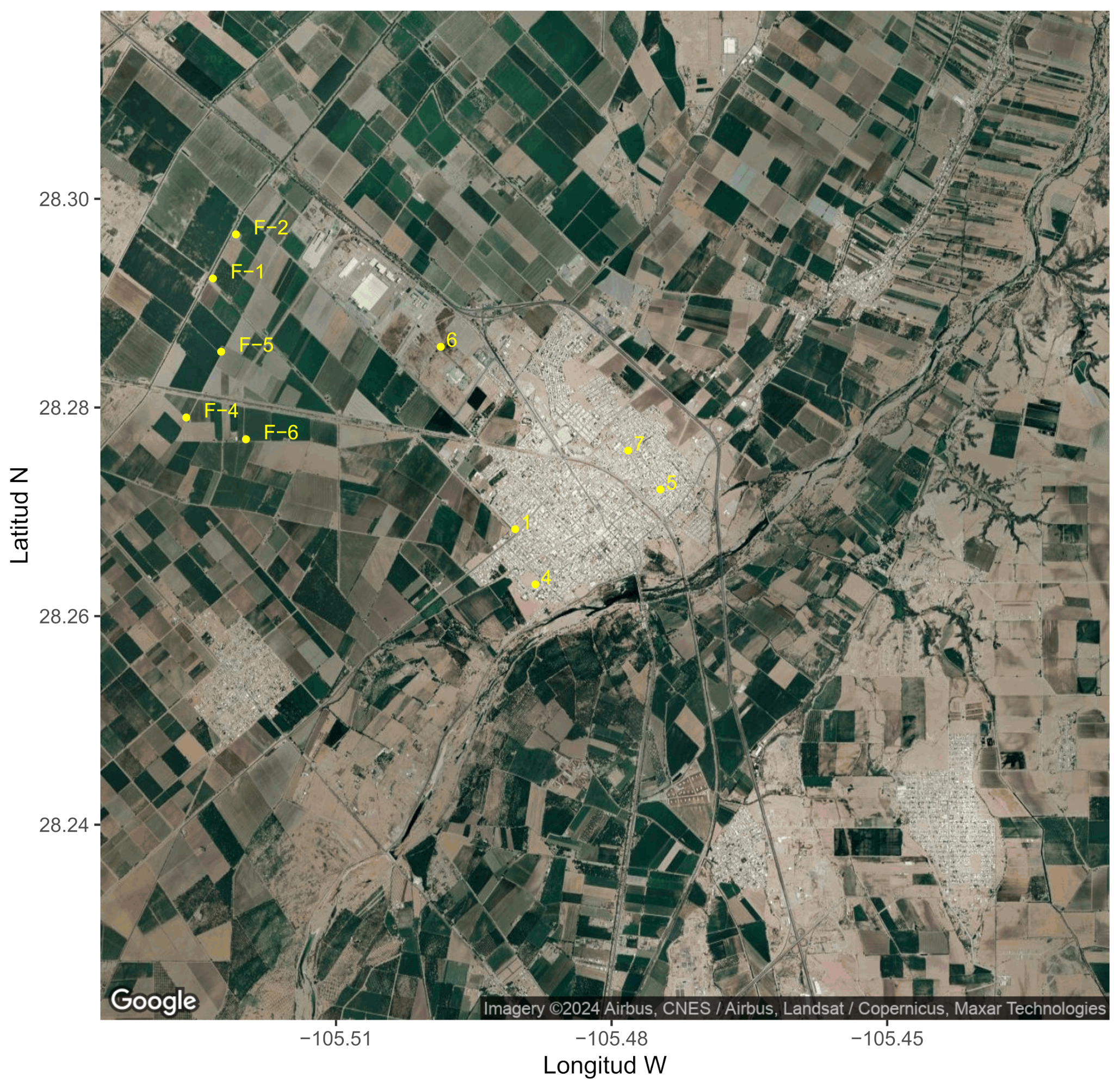
2.1. Study Site

The Chihuahuan Desert eco-region encompasses approximately 70 million ha and occupies a significant portion of the Mexican states of Chihuahua, Coahuila, Durango, and Zacatecas, as well as extensive areas of San Luis Potosí, and Nuevo León, and Texas and New Mexico in the United States [24].
The area is situated within the physiographic province of mountains and basins and is traversed by two significant rivers, the San Pedro and the Conchos, which provide a valuable resource for irrigation. The climate is semi-arid, with precipitation levels that fall below the aridity threshold but above the hyperaridity threshold. The temperature ranges from a minimum of −2 °C to a maximum of 13 °C in January, to a maximum range of 38 °C–42 °C between June and August. The municipality of Meoqui encompasses an area of 370 km2, which represents 0.149% of the total area of the state of Chihuahua. The San Pedro River Wetlands, which have been designated an RAMSAR site since 2012, are of significant ecological importance due to their high level of biodiversity and their role as a habitat for waterfowl [25]. Figure 1 offers a visual representation of the geographical position of the city of Meoqui.
The water from Meoqui has gained recognition for its palatability and quality, exhibiting a high mineral content and deemed safe for human consumption. In recent times, a number of beverage companies, including the local Refrescos Unión and multinationals Coca-Cola and Heineken Brewery, have established themselves in the vicinity of the San Pedro River.

2.2. Junta Municipal de Agua y Sameamiento (JMAS) Meoqui

JMAS is a decentralized public agency of the Government of the State of Chihuahua. The objective of the agency is to facilitate the provision of public sector services related to the treatment and distribution of drinking water in the municipality of Meoqui, Chihuahua. The agency commenced operations in 1957 under the name Junta Federal de Agua Potable.
A total of 94,000 m3 of drinking water pipes have been installed in the municipality, in addition to 80,000 m of sanitary sewerage in the municipal capital. On average, approximately 8000 m of sanitary sewers and potable water piping are installed annually, both in the municipal capital and in the rural area, as a result of maintenance activities and new constructions. The agency bears responsibility for the maintenance and construction of water and sewerage infrastructure for over 14,000 domestic, commercial, and industrial connections throughout the municipality. Of these, 8000 are situated in the municipal capital, while 6700 are located in rural areas. The provision of water services is available on a 24 h basis, and any instances of leakage are addressed in a prompt and efficient manner. Furthermore, the primary urban center is equipped with four elevated tanks, which collectively have a total storage capacity of 1150 m3 [26].

2.3. Data Collection

The data were obtained from 10 wells between the years 2006 and 2022. The wells are equipped with water meters, the data from which are stored in an Excel database on a computer at the JMAS headquarters. The data employed in this study were those pertaining to the mean monthly extraction rate. Wells F4, F5, and F6 are used to supply drinking water to the brewing industry. In addition, the wells 1, 4, 5, 6, 7, F1, and F2 provide water to a variety of sectors, including domestic, commercial, educational, public, and industrial. The water obtained from these seven wells is made potable by JMAS, and subsequently, distributed to the mentioned sectors via the municipal drinking water network. The majority of these wells are equipped with frequency variator equipment, which enables the implementation of a variable expense structure in accordance with the demand of the population. This enables the adjustment of costs in response to fluctuations in demand, thereby facilitating a more efficient and cost-effective energy supply. Figure 2 illustrates the geographical positioning of the wells.

2.3.1. Use of Urban Wells

In the context of water resource management, an “urban well” is defined as a water source that provides potable water to a range of sectors, including domestic, commercial, industrial, educational, and public use. The following section provides an overview of the utilization and defining characteristics of these wells.
Well 1 represents the historical extraction of the greatest quantity of water on an individual basis. In recent years, efforts have been made to reduce the load on this well, which has been in use for several decades and was previously able to recover from a fracture of the casing of the well.
Well 4: The final year of operation of this well was 2006, during the months of April, May, and June. The well ceased to function as a result of a collapse that impeded the extraction of water by the pumping apparatus. It was utilized exclusively for low-pressure support.
Well 5 was utilized exclusively for low-pressure support during the summer season due to the inferior quality of the water from this source. As the recently constructed wells have not yet generated sufficient revenue to offset the cost of this well, it has been used intermittently for a few hours per day to satisfy increases in demand.
Well 6 was utilized exclusively for industrial consumption in applications where the precise quality of the water was not a requisite factor. The well responded to the consumption demand of the IGP-BGD (denim washing) maquiladora, which ceased operations in January 2018.
Well 7, which has a relatively low flow rate, was initially utilized on a continuous basis. However, in certain years, it was taken out of operation during the winter season.
Well F1: The objective of the use of this well was to identify potential alternatives that would result in enhanced water quality and volume, with the aim of improving the overall water management system. At the outset of its deployment in conjunction with well F2, an increase in the dynamic level was observed, a phenomenon that was not observed when the well operated independently. In recent years, during the course of maintenance procedures, a perforation was identified in the well casing It was thus resolved to relocate the pumping apparatus to an area characterized by a blind casing.
Well F2: Initially, it was observed that this well shared a water supply with well F1. Subsequently, due to the emergence of a mechanical complication within the ademe, the well was relocated within the same property. The introduction of new drilling has not resulted in any discernible impact on the dynamic level in relation to well F1 at the present time.

2.3.2. Total Extraction

JMAS has assembled a comprehensive data set pertaining to the extraction of a total of 10 wells. The results demonstrate that the mean extraction of the aggregate of these wells during the analyzed period was 50,935 ± 47,540 m3, with a maximum value of 179,717 m3 extracted and a total of 67,233,578 during the study period (2006–2022).

2.3.3. Extraction by Type of Well

Table 2 presents the mean, standard deviation, maximum value, and total m3 extracted from the different types of well in Meoqui. The greatest quantity of m3 has been extracted from urban wells, with an average of 55,720 ± 48,865 m3 and a total of 63,520,284. Regarding the raw water wells, the quantity of extracted potable water has an average of 20,629 ± 19,767 m3 and a total of 3,713,294 m3.

2.4. Data Analyses

ARIMA models were estimated for each type of sector and in general. The R programming language (version 4.4.1) [27] was used. The R packages used are presented in Table 3.

2.5. Time-Series Methods

One of the methodologies for forecasting based on regression techniques is an approach that considers only time-dependent factors. This approach entails the formulation of predictions concerning evolutionary trends through the examination of historical data patterns. An alternative methodology is the utilization of techniques that consider the relationship between the dependent variable and the factors that influence it.
In regard to the preliminary approach, the most prevalent methodology is that of the autoregressive integrated moving average (ARIMA) models [56], in conjunction with support vector machines (SVMs) [57] and artificial neural networks (ANNs) [58]. ARIMA models have two notable disadvantages: they require a substantial amount of data smoothing and they are linear [59]. SVM models are challenging to interpret, and finally, ANNs are susceptible to local minima and overfitting issues [60]. In 2017, Facebook released an open-source algorithm for time-series prediction called Prophet [61], which is based on time-series decomposition and is capable of handling outliers related to special events such as holiday periods. For instance, Prophet has been utilized in conjunction with ARIMA in domains such as weather [62] and epidemiology [63].
In the context of the second case, the most frequently utilized methodologies are regression analysis (RA) [64] and SVMs [65] . One of the limitations of these methodologies is their lack of computational efficiency when applied to large amounts of data. Recently, some intelligent algorithms, such as deep learning and neural networks, have been employed to address this issue. However, the predictive efficiency of these algorithms is contingent upon the quantity of input data, thereby necessitating computational equipment with substantial storage and processing capacity [66]. Deep learning has been demonstrated to yield highly accurate predictions and its training process is notably efficient, particularly in scenarios where data are limited. Among the ensemble learning techniques are bagging and boosting [67]. In the initial case, the most frequently utilized algorithm is random forest, which is primarily employed for classification rather than regression problems [68]. The gradient boosting decision tree (GBDT) algorithm has been demonstrated to be proficient in boosting [69]; however, its processing of high-dimensional data is hindered by a notable deficiency in parallel computational operations. Chen and Guesrin Chen and Guestrin [70] proposed the extreme gradient boosting (XGBoost) method, which is based on GBDT, as a potential solution to this limitation. This method has been demonstrated to exhibit highly robust predictive performance.
To illustrate, the ARIMA model is constrained to capturing linear features, and is thus frequently integrated with algorithms such as SVM [71,72] and neural networks [72,73] to enhance its predictive precision by encompassing both linear and nonlinear features. Moreover, a multitude of hybrid models have been devised based on methodologies with disparate weight determination processes [74].
The aforementioned algorithms have been demonstrated to be effective in a range of applications across diverse fields. However, they are particularly adept at handling non-stationary and nonlinear data of a fluctuating nature, which presents significant challenges for a single model to overcome. This has led to the development of hybrid models, which integrate multiple models to achieve enhanced performance.

2.5.1. Train/Test

  • Split time series into training and testing sets.
  • Make a train/test set (12 months).
  • Visualize the train/test split.
  • Modeling.
Model equation:
m 3 d a t e , t r a i n i n g ( s p l i t s )
  • ‘Auto ARIMA’ function from forecast.
  • ‘Prophet’ algorithm from Prophet.

2.5.2. Machine Learning Models

The complexity of machine learning models is greater than that of automated models. This complexity typically necessitates the implementation of a workflow, which is sometimes referred to as a pipeline in other languages. The general process can be described as follows:
  • Create preprocessing recipe.
  • Create model specifications.
  • Use workflow to combine model specifications and preprocessing, and fit model.

2.5.3. Preprocessing Recipe

A preprocessing ‘recipe’ was devised, incorporating time-series steps. The process employed the ‘date’ column to generate novel features that are subsequently modeled. These features included those derived from time series and Fourier series.

2.5.4. Prophet Boost

The Prophet Boost algorithm represents a novel approach to data analysis, whereby the Prophet algorithm is integrated with the XGBoost machine learning model. The objective of this integration is to leverage the strengths of both Prophet and XGBoost, thereby creating a more robust and automated data analysis process. The algorithm operates as follows: The univariate series is initially modeled using the Prophet algorithm. Subsequently, the regressors are provided via the preprocessing recipe, and the Prophet residuals are regressed with the XGBoost model. A workflow may be established for the model in a manner analogous to that employed for machine learning algorithms.

2.5.5. The Modeltime Workflow

Modeltime. The workflow has been designed with the objective of accelerating the evaluation and selection of models. Given the availability of multiple time-series models, it is now possible to undertake an analysis of these models and to make forecasts about future outcomes using the modeltime approach.
Workflow
  • Modeltime table. The modeltime table employs a system of identification numbers and the creation of generic descriptions to assist in the organization and tracking of models.
  • Calibration. Model calibration is utilized to quantify errors and estimate confidence intervals. Model calibration was conducted on the out-of-sample data set (also referred to as the testing set) to generate the actual values, fitted values, and residuals for the testing set.
  • Forecast (testing set).
    • The calibration of data allows for the visualization of testing predictions, which may be regarded as a forecast.
    • The subsequent step is to calculate the accuracy of the testing process in order to facilitate a comparison of the models.
  • Analyze results. The optimal model is selected based on an evaluation of the accuracy measures and forecast results.
  • Model evaluation and selection. In the field of data science and machine learning, the assessment of predictive model performance is of paramount importance. In the context of regression problems, where the objective is to predict continuous numerical values, one of the fundamental metrics employed for evaluation is the mean absolute error (MAE).
The root mean square error (RMSE) is defined as the square root of the mean of the squared deviations between the expected and observable values. It is a valuable tool in situations where the occurrence of significant errors is to be avoided. As the square of the error is taken before averaging, discrepancies of a considerable magnitude are penalized. In this context, the RMSE is an appropriate metric for forecasting extractions with minimal error (i.e., penalizing significant errors). Consequently, the RMSE has been employed to assess and corroborate the efficacy of the disparate models utilized.
The coefficient of determination (RSq) is a statistical measure that quantifies the extent to which the variation in a dependent variable can be explained by a given independent variable.
The models (SARIMA, Facebook Prophet, and Facebook Prophet Boost) were trained and calibrated using a one year data and subsequently evaluated. For model selection, the MAE, RMSE, and RSq values were used.
As previously stated in Section 2.4, the R statistical package Modeltime was employed for the purposes of analysis. This is a recently developed time-series forecasting package designed to facilitate the evaluation, selection, and forecasting of models. Modeltime achieves this by integrating the tidymodels machine learning package ecosystem into an optimized forecasting workflow, collectively known as the tidyverse. The initial step involves the partitioning of the data set through the use of the time_series_split() function, which facilitates the creation of a train/test set utilizing the final 12 months of data as the testing set.
The subsequent step is to estimate the models and create a table with the resulting estimates. Subsequently, the models are calibrated on the out-of-sample data (i.e., the testing set) with the modeltime_calibrate() function. A new data set is created with the actual values, fitted values, and residuals for the testing set, which allows for a comprehensive examination of the data. Once the data have been calibrated, it is possible to generate a visual representation of the testing predictions, or forecast.
Subsequently, the testing accuracy can be calculated in order to facilitate a comparison of the models. The out-of-sample accuracy metrics were generated using the modeltime_accuracy() function, and the best models were selected based on these metrics.
6.
Refitting. Models are refitted as a best practice prior to forecasting the future. Subsequently, a process of retraining on comprehensive data sets is undertaken. As the models are dependent on the ‘date’ feature, the option ‘h’ (horizon) is employed for forecasting purposes. This value was set to ‘12 months’ in order to forecast the following 12 months of data.

3. Results

Table 4 depicts the ARIMA models estimated for each well and the Akaike information criterion corrected (AICc). It is important to acknowledge that the estimated models may vary from one well to another due to the differing management approaches employed in each case, as referenced in Section 2.3.1. Moreover, the results are presented in detail for general consumption and two groups of wells were created based on the users, the status of their connection to the water network, and the treatment of the water by JMAS in Meoqui. The initial group comprises those wells that are situated primarily in the urban area and connected to the general drinking water network, designated as ‘urban wells’. The second one is ‘raw water wells’ that provide water to the brewery industry and are situated outside the urban area, thus not supplying the general drinking water network.

3.1. Time-Series Analysis

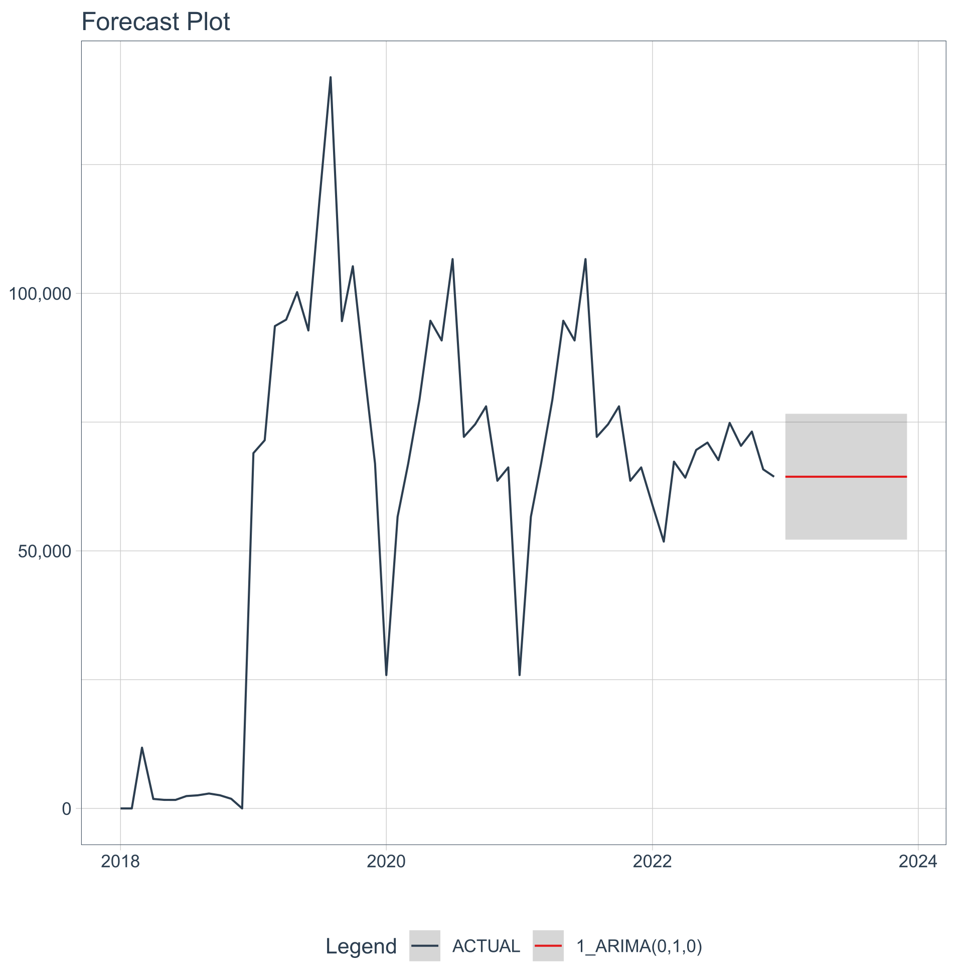
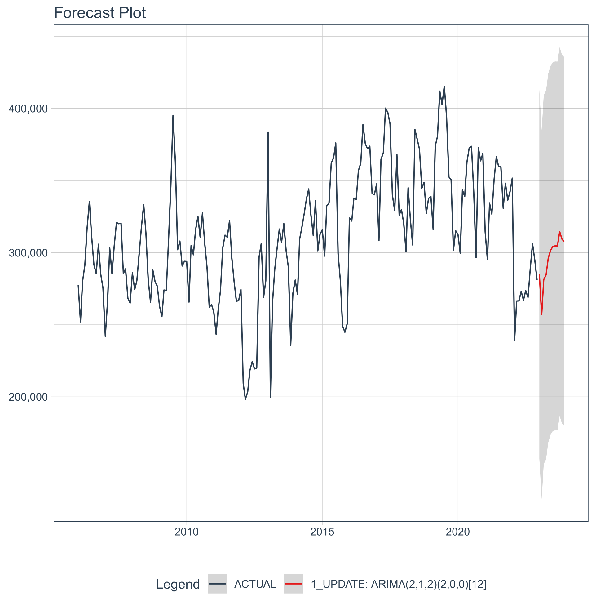
3.1.1. Extraction from All the Wells

Table 5 presents the values of MAE, RMSE, and RSq. It can be observed that the SARIMA model yields the best results for model selection. Based on these findings, the SARIMA(1,1,1) (1,0,0)12 is identified as the optimal model for ’extraction from all the wells’. The MAE value of the model is 41% better than the Prophet model and 24% than Prophet Boost; the RMSE was 43% and 27% better, respectively.
The results of the calibrated model and one-year forecast are presented in Figure 3. In accordance with the Mann–Kendall trend test, the value of S = 10974 indicates a monotonic increase in the general water extraction. The projected value of Sen’s slope [z = 10.334, n = 216, p-value < 0.001] is estimated to be 561.36 for the time series.
Graphical and tabular results of the SARIMA model and a one-year forecast for the total extraction of potable water from wells in Meoqui, Chihuahua, Mexico, are presented in Figure 3 and Table 6, which illustrate the predicted values and their respective intervals on a monthly basis over the course of a year. The maximum predicted extraction is 368,019.1 m3, 95% CI [218,087.3, 517,950.8], in October and the minimum is 319,435.8 m3, 95% CI [169,504.1, 469,367.6], in February.

3.1.2. Raw Water Wells

An ARIMA(0,1,0), or ’white noise’, model was identified as the best model for raw water wells. The MAE was 776% better than the Prophet model and 465% better than Prophet Boost; the RMSE was 596% and 383% better, respectively (Table 7).
In accordance with the projected value of Sen’s slope, it is anticipated that there will be no increase in the volume of water extracted from these wells, in accordance with the Mann–Kendall trend test, which indicated no monotonic changes (z = 0.35119, n = 72, p-value = 0.7254). This can be attributed to the stabilization and improvement in production processes in the local brewing industry, which has resulted in a more efficient utilization of the supplied water and production stabilization.
The results of the ARIMA model and the one-year forecast for the extraction of potable water from ‘urban wells’ in Meoqui, Chihuahua, Mexico, are presented in Figure 4 and Table 8. This Table illustrates the predicted values are 64,399 m3, and their respective intervals are 95% CI [52,179.3, 76,618.7] on a monthly basis over the course of a year.

3.1.3. Urban Wells

Table 9 shows that an SARIMA model was identified as the optimal choice for ’urban wells’. The MAE value of the model is 28% better than the Prophet model and 26% better than Prophet Boost; the RMSE is 33% and 32% better, respectively. These findings were obtained after the calibration of the models. The estimated model was SARIMA(2,1,1)(2,0,0)12.
The initial segment of the model indicates that the autocorrelation is two months (AR2) and that the variability is one month. In order to achieve stationarity, the data set was differenced. In the seasonal component, an MA2 was estimated. In accordance with the Mann–Kendall trend test (S = 5554), a monotonic increase was estimated, while the value of Sen’s slope was 249.78 [z = 5.2297, n = 216, p-value < 0.001], indicating an increase in the time series.
The results of the SARIMA model and the one-year forecast for the extraction of potable water from urban wells in Meoqui, Chihuahua, Mexico, are presented in Figure 5 and Table 10, which illustrate the predicted values and their respective intervals on a monthly basis over the course of a year. The maximum predicted extraction is 314,587.4 m3, 95% CI [186,670.0, 442,504.7], in October and the minimum is 257,007.1 m3, 95% CI [129,089.8, 384,924.5], in February.

4. Discussion

In order to ascertain which model exhibits the greatest forecasting capacity for assessing the pattern in groundwater extraction, three models of seasonal autoregressive integrated moving average (SARIMA) were evaluated. The models subjected to evaluation were Prophet, Prophet with extreme gradient boosting (XGBoost), and Prophet with XGBoost and seasonal autoregression. The ARIMA model exhibited the greatest forecasting capacity for all three types of groundwater extraction: general extraction, extraction of raw water, and urban potable water use. In this regard, numerous authors concur that the ARIMA model is the most efficient for hydrological forecasting.
In a study conducted by Azad et al. [75] in the Red Hills Reservoir (RHR), a primary source of potable and irrigation water in Thiruvallur district, Tamil Nadu, India, the findings indicated that the SARIMA-ANN hybrid model demonstrated superior performance compared to the remaining models with respect to all performance criteria for reservoir water level prediction. In light of these findings, the authors conclude that the SARIMA-ANN hybrid model represents a promising approach for accurate reservoir water level prediction. In Iran, Ahmadpour et al. [76] evaluated the efficacy of four models—a classical multilayer perceptron neural network, SARIMA, a nonlinear time-series model, and an SARIMA-BL hybrid time-series model—in predicting and modeling monthly qualitative parameters, such as those observed in the Maroon River in Iran. The findings indicated that the SARIMA-ANN hybrid model demonstrated superior performance compared to the remaining models across all performance criteria for predicting reservoir water reserve level.
Yang et al. [77] sought to predict the volume of water entering a Laohutai mine in Liaoning, China, with two objectives: to ensure the safety of workers and to protect the environment. The GC-SARIMA-LSTM model exhibited superior performance compared to the Visual MODFLOW numerical simulation software in predicting the mine water inflow. In other study, Liu et al. [78] conducted an evaluation of a number of models. The models subjected to evaluation were autoregressive integrated moving average (ARIMA), a neural network (NN), random forest (RF), and Prophet. The findings indicate that data-centric machine learning methodologies are characterized by four key features; these methodologies have the potential to enhance the precision of short-term water demand projections. With a relatively limited amount of training data, precise forecasts can be achieved. The RF and NN models demonstrate superior performance in forecasting high-resolution temporal data. Furthermore, enhancing data quality can result in a level of accuracy that is comparable to that achieved by model-centric machine learning methodologies. Another example of a model test is the study conducted by Rajballie et al. [64], who evaluated the efficacy of various statistical models for forecasting water consumption in Trinidad. The models included in the study were seasonal ARIMA, exponential state space (ETS), and artificial neural network (ANN) models, as well as hybrid combinations of these approaches. The findings indicated that the hybrid model combinations were effective for forecasting four of the five consumption values.
Another illustrative example of a model test is the study conducted by Rajballie et al. [79], in which the efficacy of various statistical models for forecasting water consumption in Trinidad was evaluated. The models included in the study were seasonal ARIMA, exponential state space (ETS), and artificial neural network (ANN) models, as well as hybrid combinations of these approaches. The findings indicated that the hybrid model combinations were effective for forecasting four of the five consumption categories. As demonstrated by the aforementioned authors, the SARIMA model represents an effective methodology for forecasting water levels. The working hypothesis states that the volume of water extracted over time can be explained by a statistical time-series model for the purpose of forecasting future trends. This hypothesis suggests a temporal shift in the volume of water extracted over time in wells managed by JMAS Meoqui. To test the aforementioned hypothesis, a time-series approach was employed, whereby ARIMA models, Facebook Prophet, and a hybrid model, Prophet Boost, were tested in order to leverage the efficacy of these models in the presence of seasonality. In a related study, Roy et al. [7] put forth the proposition that the findings will contribute to more efficient water resource management.
The application of modeling will facilitate the identification of trends and enable the prediction of fluctuations in groundwater levels. Furthermore, the root causes of these fluctuations can be identified, as can their projected direction and characteristics. This is the first study employing a time-series approach, which enables the projection of groundwater extraction through wells in Meoqui, Chihuahua. The findings will furnish the requisite data to enhance water management practices in this municipality, particularly given that groundwater, an indispensable component of the hydrosphere, sustains water flow during periods of precipitation deficit and represents a pivotal source of freshwater supply [80]. The quantification of groundwater levels is of paramount importance because it allows the state of water resources to be assessed. The results of our study will allow better management of water resources, since, from the modeling, it will be possible to predict groundwater fluctuations and know the causes and the direction and characteristics of the trends [7]; unfortunately, in less developed economies it is common to observe not only a lack of financial resources but also a low priority given to water and sanitation; in addition, corruption and lack of transparency limit effective water management [81].
The extraction volumes analyzed were the monthly total per well and the general total. The mean volume of water extracted from all wells during the period under analysis was 50,935 ± 47,540 m3, with a total of 67,233,578 m3 withdrawn. The greatest quantity of water extracted historically was from well 1, with an average volume of 131,960 ± 31,656 m3. In regard to the time-series analysis, an SARIMA (1,1,1)(1,0,0)12 model was estimated for the general extraction. The initial component of the model indicates that the extraction for a given month is influenced by the preceding month (AR1). There is a discernible tendency towards increased water withdrawal, accompanied by a small variation over the course of a single month (MA1). In contrast, the seasonal AR1 component is presented, exhibiting no discernible trend or variation. In accordance with the Mann–Kendall trend test, the value of S = 10974 indicates a monotonic increase. The value of Sen’s slope (z = 10.334, n = 216, p-value < 0.001), for the time series has a positive slope of 561.36. The observed increase in water extraction may be indicative of an increase in water demand, a phenomenon previously documented by Neme et al. [82]. These researchers have observed that, while the country’s average annual water supply is approximately 67 billion m3, demand exceeds 78 billion m3, with this gap projected to reach 23 billion m3 per year by 2030.
The pattern of the wells utilized by the brewing industry evinces a period of stabilization, followed by a subsequent decline in recorded extraction. The estimated model was an ARIMA(0,1,0). No discernible trend was identified for these wells. It is of the utmost importance that future studies identify not only the current consumption of these aquifers, where stable extraction has been achieved, but also determine their capacity to meet future demands. As stated by MacAllister [5], a decline in groundwater levels was observed in 30% of the aquifer systems during the 21st century. Furthermore, the depletion of these resources was more prevalent and rapid in cultivated drylands, which are characteristics typical of the ecosystem in Meoqui, Chihuahua. Conversely, measures that promote water circularity should be reinforced, such as the utilization of treated wastewater, which has the potential to mitigate the discrepancy between water supply and demand. As projected, the volume of wastewater is expected to reach 9.2 billion m3 by 2030. If treated and subsequently reused, this could potentially result in a reduction of demand by 40% (Fund for Communication and Education (FCA)) [83].
In contrast with the observations in the wells utilized by the brewing industry, an SARIMA(2,1,1)(2,0,0)12 model was developed for the wells that supply the urban drinking water network to users in the commercial, domestic, industrial, school, and public sectors. It is anticipated that the volume of withdrawals will increase over time, reflecting an anticipated rise in demand. In accordance with the projected value of the Mann–Kendall trend test (S = 5554), a monotonic increase is present and the Sen’s slope [z = 5.2297, n = 216, p-value < 0.001], indicates a positive trend in the time series of 249.78 m3 per month. As stated in Larraz et al. [84], in regions and periods experiencing water scarcity, and in light of the climate emergency, it is crucial to consider the environmental and social implications of water usage across various economic sectors.
In their 2020 study, Rahim and colleagues [85] identified four key factors that contribute to the phenomenon of water scarcity. (1) Uneven geographic distribution of water sources; (2) rapid urbanization leading to population and economic growth; (3) inadequate management of water resources; and (4) prolonged drought. All of these factors are present in the region of Meoqui, Chihuahua, thereby providing a compelling rationale for continued investigation into the dynamics of the water wells that supply water to the urban population. The findings of this research will inform the development of strategies to prevent the scarcity of this resource and satisfy the demand of the population of Meoqui, Chihuahua. The extraction of groundwater has been observed to exhibit different trends across time due to the establishment of companies that require water for their operations, particularly for drinking purposes. In one instance, the closure of a company resulted in a notable alteration to the overall extraction patterns. A distinctive pattern can be discerned in the context of well withdrawals in the city of Meoqui, Chihuahua. There is an upward trend in extractions that begins in 2013, followed by a period of stabilization until 2020. This stabilization can be attributed to industrial sector operations. One of the plants was engaged in the unwashing of denim garments. It is notable that the well in question did not comply with the current regulations pertaining to human consumption. The cessation of operations at the plant occurred concurrently with the commencement of brewery industry activities. The sector is supplied with water from three distinct wells, which resulted in a stabilization of the volume of extractions from 2018 to 2020. In that year, production in the brewing sector reached a point of equilibrium, resulting in a decline in extraction. Nevertheless, the model suggests an anticipated increase in water withdrawals.
Conversely, advancements in well technology have facilitated enhanced management capabilities, enabling precise control over the extraction process. Furthermore, in contrast to the management of the wells in the past, which was primarily focused on supplying the city with a single well, with others only activated during periods of increased demand (such as summer), the current approach involves a more distributed approach to well management.
From the main results obtained, it is clear that governmental consortia, businesses, industries, health and financial organizations, environmental organizations, educational institutions, and research centers must prioritize the resolution of water-related issues [86], particularly those confronting organizations dedicated to water management. The last of these is crucial to guarantee the sustainability of water supply and sanitation [85]. Moreover, it is essential to seek collaborative partnerships to develop integrated solution strategies that take into account the multifaceted dimensions of cultural, environmental, and economic conditions, with the objective of achieving comprehensive global coverage of the aforementioned services [3].
The main outcomes generated from our study regarding aquifer utilization in one characteristic semi-arid eco-region in northern Mexico, represent a significant advantage for the region in terms of water use sustainability. Undoubtedly, as proposed by Katic and Grafton [87], an effective groundwater management depends on precise estimates of past and current groundwater extraction. However, these measurements are not publicly available in the majority of areas worldwide due to a range of factors, including physical, regulatory, and social challenges.
The principal findings of our study on the utilization of aquifers in a distinctive semi-arid eco-region in northern Mexico demonstrate a significant benefit for the region in terms of water use sustainability. As Katic and Grafton [87] have observed, effective groundwater management depends on precise estimates of past and current groundwater extraction. However, these measurements are not publicly available in the majority of areas worldwide due to a range of factors, including physical, regulatory, and social challenges.
In consideration of the intrinsic constraints of this study, the following limitations can be identified: Notwithstanding the region’s semi-arid climate, with low precipitation and high temperatures, this study did not incorporate climatic variables. Furthermore, an evaluation of water use efficiency was not possible. Such an objective could have been achieved through the quantification of the volume of water extracted from wells and that which reaches consumers. It would be beneficial for future research to consider the quality of the water supplied to consumers. Furthermore, it would be advantageous to incorporate spatial variations in water consumption, which were not considered in this study.

5. Conclusions

Empirical evidence substantiates the efficacy of the SARIMA model for forecasting water levels. In consequence, the volume of water extracted over time can be explained by a statistical time-series model for forecasting future trends.
In this region, the extraction for a given month is influenced by the preceding month, exhibiting a discernible tendency towards increased water withdrawal. However, this is accompanied by a slight variation over the course of a single month, which is not discernible as a trend or variation.
It is recommended that municipal authorities and water managers collaborate with users to develop policies that ensure the sustainability of the resource. Although the wells utilized by the brewing industry have exhibited a period of stabilization, with subsequent declines in recorded extraction, it is anticipated that the urban drinking water network will experience an increase in the volume of withdrawals, which will be reflected in an increase in demand. Such circumstances could potentially give rise to disputes between users regarding the utilization of the resource.
Further research could investigate additional computational intelligence techniques, including threshold auto-excited autoregressive models, multivariate adaptive regression splines, and random forests. Such an approach could be undertaken with the objective of comparing and enhancing the models in question.

Author Contributions

Conceptualization, M.A.L.-G.; methodology, M.A.L.-G.; software, M.A.L.-G.; validation, M.A.L.-G. and V.C.-V.; formal analysis, M.A.L.-G.; investigation, M.A.L.-G., R.R.-M., D.L.-G. and C.S.C.-T.; data curation, M.A.L.-G., R.R.-M. and D.L.-G.; writing—original draft preparation, M.A.L.-G. and R.R.-M.; writing—review and editing, C.A.M.-H., R.R.-M., C.S.C.-T., V.C.-V. and F.G.V.-D.; visualization, M.A.L.-G.; supervision, F.G.V.-D.; project administration, F.G.V.-D. All authors have read and agreed to the published version of the manuscript.

Funding

This research received no external funding.

Institutional Review Board Statement

Not applicable.

Informed Consent Statement

Not applicable.

Data Availability Statement

Data may be available from JMAS Meoqui through the Mexican Instituto Federal de Acceso a la Información (IFAI).

Acknowledgments

Mexican Consejo Nacional de Humanidades Ciencia y Tecnología (CONAHCYT) for first author postdoctoral fellowship. Junta Municipal de Aguas y Saneamiento (JMAS) of Meoqui, Chihuahua, Mexico, through its Jefatura de Sistemas for providing the data for this research.

Conflicts of Interest

The authors declare no conflicts of interest.

Abbreviations

The following abbreviations are used in this manuscript:
AICcAkaike information criterion corrected
ARIMAAutoregressive integrated moving average
CONAHCYTConsejo Nacional de Humanidades, Ciencia y Tecnología
CIConfidence interval
IFAIInstituto Federal de Acceso a la Información
JMASJunta Municipal de Aguas y Saneamiento
MAEMean average error
RSqR-squared (coefficient of determination)
RMSERoot mean square error
SARIMASeasonal autoregressive integrated moving average
WHOWorld Health Organization

References

  1. Peydayesh, M.; Mezzenga, R. Protein nanofibrils for next generation sustainable water purification. Nat. Commun. 2021, 12, 3248. [Google Scholar] [CrossRef] [PubMed]
  2. Buttinelli, R.; Cortignani, R.; Caracciolo, F. Irrigation water economic value and productivity: An econometric estimation for maize grain production in Italy. Agric. Water Manag. 2024, 295, 108757. [Google Scholar] [CrossRef]
  3. Postel, S.L. Water and world population growth. J. Am. Water Work. Assoc. 2000, 92, 131–138. [Google Scholar] [CrossRef]
  4. Stockholm Environment Institute. 6 Clean Water and Sanitation. 2024. Available online: https://www.government.se/contentassets/0be76988b3444b0881b6513daaf5bb26/6---Clean-water-and-sanitation.pdf (accessed on 1 September 2024).
  5. MacAllister, D.J. Groundwater Decline is Global but Not Universal. 2024. Available online: https://www.nature.com/articles/d41586-024-00070-3 (accessed on 1 September 2024).
  6. Henao, C.; Lis-Gutiérrez, J.P.; Lis-Gutiérrez, M.; Ariza-Salazar, J. Determinants of efficient water use and conservation in the Colombian manufacturing industry using machine learning. Humanit. Soc. Sci. Commun. 2024, 11, 1–11. [Google Scholar] [CrossRef]
  7. Roy, S.; Taloor, A.K.; Bhattacharya, P. A geospatial approach for understanding the spatio-temporal variability and projection of future trend in groundwater availability in the Tawi basin, Jammu, India. Groundw. Sustain. Dev. 2023, 21, 100912. [Google Scholar] [CrossRef]
  8. Yagbasan, O.; Demir, V.; Yazicigil, H. Trend Analyses of Meteorological Variables and Lake Levels for Two Shallow Lakes in Central Turkey. Water 2020, 12, 414. [Google Scholar] [CrossRef]
  9. Tejada, A., Jr.; Talento, M.S.; Ebal, L.P.; Villar, C.; Dinglasan, B.L. Forecasting of Monthly Closing Water Level of Angat Dam in the Philippines: SARIMA Modeling Approach. J. Environ. Sci. Manag. 2023, 26, 42–51. [Google Scholar] [CrossRef]
  10. Niknam, A.; Zare, H.K.; Hosseininasab, H.; Mostafaeipour, A.; Herrera, M. A Critical Review of Short-Term Water Demand Forecasting Tools—What Method Should I Use? Sustainability 2022, 14, 5412. [Google Scholar] [CrossRef]
  11. Zafra-Mejía, C.A.; Rondón-Quintana, H.A.; Urazán-Bonells, C.F. ARIMA and TFARIMA Analysis of the Main Water Quality Parameters in the Initial Components of a Megacity’s Drinking Water Supply System. Hydrology 2024, 11, 10. [Google Scholar] [CrossRef]
  12. Agaj, T.; Budka, A.; Janicka, E.; Bytyqi, V. Using ARIMA and ETS models for forecasting water level changes for sustainable environmental management. Sci. Rep. 2024, 14, 22444. [Google Scholar] [CrossRef]
  13. Barrientos-Torres, D.; Martinez-Ríos, E.A.; Navarro-Tuch, S.A.; Pablos-Hach, J.L.; Bustamante-Bello, R. Water Flow Modeling and Forecast in a Water Branch of Mexico City through ARIMA and Transfer Function Models for Anomaly Detection. Water 2023, 15, 2792. [Google Scholar] [CrossRef]
  14. Silva, A.C.d.; Silva, F.d.G.B.d.; Valério, V.E.d.M.; Silva, A.T.Y.L.; Marques, S.M.; Reis, J.A.T.d. Application of data prediction models in a real water supply network: Comparison between arima and artificial neural networks. RBRH 2024, 29, e12. [Google Scholar] [CrossRef]
  15. Cheema, M.A.; Hanif, M.; Albalawi, O.; Mahmoud, E.E.; Nabi, M. Evaluating water-related health risks in East and Central Asian Islamic Nations using predictive models (2020–2030). Sci. Rep. 2024, 14, 16837. [Google Scholar] [CrossRef] [PubMed]
  16. Zuo, H.; Gou, X.; Wang, X.; Zhang, M. A Combined Model for Water Quality Prediction Based on VMD-TCN-ARIMA Optimized by WSWOA. Water 2023, 15, 4227. [Google Scholar] [CrossRef]
  17. Jesus, E.d.S.d. Modelos de aprendizagem de máquina para previsão da demanda de água da região metropolitana de Salvador, Bahia. Neural Comput. Appl. 2023, 35, 19669–19683. [Google Scholar] [CrossRef]
  18. Niknam, A.R.R.; Sabaghzadeh, M.; Barzkar, A.; Shishebori, D. Comparing ARIMA and various deep learning models for long-term water quality index forecasting in Dez River, Iran. Environ. Sci. Pollut. Res. 2024. [CrossRef]
  19. Jaya, N.A.; Arsyad, M.; Palloan, P. Estimation of Groundwater River Availability in Leang Lonrong Cave Using ARIMA Model and Econophysics Valuation Approach. Adv. Soc. Humanit. Res. 2024, 2, 737–754. [Google Scholar] [CrossRef]
  20. Xu, J. Forecasting Water Demand With the Long Short-Term Memory Deep Learning Mode. Int. J. Inf. Technol. Syst. Approach (IJITSA) 2024, 17, 1–18. [Google Scholar] [CrossRef]
  21. Drogkoula, M.; Kokkinos, K.; Samaras, N. A Comprehensive Survey of Machine Learning Methodologies with Emphasis in Water Resources Management. Appl. Sci. 2023, 13, 2147. [Google Scholar] [CrossRef]
  22. Aquil, M.A.I.; Ishak, W.H.W. Comparison of Machine Learning Models in Forecasting Reservoir Water Level. J. Adv. Res. Appl. Sci. Eng. Technol. 2023, 31, 137–144. [Google Scholar] [CrossRef]
  23. Pires, C.; Martins, M.V. Enhancing Water Management: A Comparative Analysis of Time Series Prediction Models for Distributed Water Flow in Supply Networks. Water 2024, 16, 1827. [Google Scholar] [CrossRef]
  24. Dinerstein, E.; Olson, D.; Atchley, J.; Loucks, C.; Contreras-Balderas, S.; Abell, R.; Iñigo-Elias, E.; Enkerlin, E.; Williams, C.; Castilleja, G. Ecoregion-Based Conservation in the Chihuahuan Desert: A Biological Assessment, 2nd ed.; World Wildlife Fund (WWF): Washington, DC, USA, 2001; p. 92. [Google Scholar]
  25. Legarreta-González, M.A.; Meza-Herrera, C.A.; Rodríguez-Martínez, R.; Chávez-Tiznado, C.S.; Véliz-Deras, F.G. Time Series Analysis to Estimate the Volume of Drinking Water Consumption in the City of Meoqui, Chihuahua, Mexico. Water 2024, 16, 2634. [Google Scholar] [CrossRef]
  26. JMAS Meoqui. Junta Municipal de Aguas y Saneamiento Meoqui. Available online: http://www.jmasmeoqui.gob.mx/historia.html (accessed on 1 September 2024).
  27. R Core Team. R: A Language and Environment for Statistical Computing. 2024. Available online: https://www.R-project.org/ (accessed on 1 September 2024).
  28. Robinson, D.; Hayes, A.; Couch, S. broom: Convert Statistical Objects into Tidy Tibbles. R Package Version 1.0.6. 2024. Available online: https://CRAN.R-project.org/package=broom (accessed on 19 September 2024).
  29. Kuhn, M.; Frick, H. dials: Tools for Creating Tuning Parameter Values. 2024. R Package Version 1.3.0. Available online: https://CRAN.R-project.org/package=dials (accessed on 19 September 2024).
  30. Wickham, H.; François, R.; Henry, L.; Müller, K.; Vaughan, D. dplyr: A Grammar of Data Manipulation. 2023. R Package Version 1.1.4. Available online: https://CRAN.R-project.org/package=dplyr (accessed on 19 September 2024).
  31. Kahle, D.; Wickham, H. ggmap: Spatial Visualization with ggplot2. R J. 2013, 5, 144–161. [Google Scholar] [CrossRef]
  32. Wickham, H. ggplot2: Elegant Graphics for Data Analysis; Springer: New York, NY, USA, 2016. [Google Scholar]
  33. Couch, S.P.; Bray, A.P.; Ismay, C.; Chasnovski, E.; Baumer, B.S.; Çetinkaya Rundel, M. infer: An R package for tidyverse-friendly statistical inference. J. Open Source Softw. 2021, 6, 3661. [Google Scholar] [CrossRef]
  34. Grolemund, G.; Wickham, H. Dates and Times Made Easy with lubridate. J. Stat. Softw. 2011, 40, 1–25. [Google Scholar] [CrossRef]
  35. Kuhn, M. modeldata: Data Sets Useful for Modeling Examples. R Package Version 1.4.0. 2024. Available online: https://CRAN.R-project.org/package=modeldata (accessed on 19 September 2024).
  36. Dancho, M. modeltime: The Tidymodels Extension for Time Series Modeling. R Package Version 1.3.0. 2024. Available online: https://CRAN.R-project.org/package=modeltime (accessed on 19 September 2024).
  37. Kuhn, M.; Vaughan, D. parsnip: A Common API to Modeling and Analysis Functions. R Package Version 1.2.1. 2024. Available online: https://CRAN.R-project.org/package=parsnip (accessed on 19 September 2024).
  38. Wickham, H.; Henry, L. purrr: Functional Programming Tools. R Package Version 1.0.2. 2023. Available online: https://CRAN.R-project.org/package=purrr (accessed on 19 September 2024).
  39. Wickham, H.; Hester, J.; Bryan, J. readr: Read Rectangular Text Data. R Package Version 2.1.5. 2024. Available online: https://CRAN.R-project.org/package=readr (accessed on 19 September 2024).
  40. Kuhn, M.; Wickham, H.; Hvitfeldt, E. recipes: Preprocessing and Feature Engineering Steps for Modeling. R Package Version 1.1.0. 2024. Available online: https://CRAN.R-project.org/package=recipes (accessed on 19 September 2024).
  41. Wickham, H. Reshaping Data with the reshape Package. J. Stat. Softw. 2007, 21, 1–20. [Google Scholar] [CrossRef]
  42. Frick, H.; Chow, F.; Kuhn, M.; Mahoney, M.; Silge, J.; Wickham, H. rsample: General Resampling Infrastructure. R Package Version 1.2.1. 2024. Available online: https://CRAN.R-project.org/package=rsample (accessed on 19 September 2024).
  43. Wickham, H.; Pedersen, T.L.; Seidel, D. scales: Scale Functions for Visualization. R Package Version 1.3.0. 2023. Available online: https://CRAN.R-project.org/package=scales (accessed on 19 September 2024).
  44. Wickham, H. stringr: Simple, Consistent Wrappers for Common String Operations. 2023. R Package Version 1.5.1. Available online: https://CRAN.R-project.org/package=stringr (accessed on 19 September 2024).
  45. Müller, K.; Wickham, H. tibble: Simple Data Frames. R Package Version 3.2.1. 2023. Available online: https://CRAN.R-project.org/package=tibble (accessed on 19 September 2024).
  46. Kuhn, M.; Wickham, H. Tidymodels: A Collection of Packages for Modeling and Machine Learning Using Tidyverse Principles. 2020. Available online: https://www.tidymodels.org (accessed on 19 September 2024).
  47. Wickham, H.; Vaughan, D.; Girlich, M. tidyr: Tidy Messy Data. 2024. R Package Version 1.3.1. Available online: https://CRAN.R-project.org/package=tidyr (accessed on 19 September 2024).
  48. Wickham, H.; Averick, M.; Bryan, J.; Chang, W.; McGowan, L.D.; François, R.; Grolemund, G.; Hayes, A.; Henry, L.; Hester, J.; et al. Welcome to the tidyverse. J. Open Source Softw. 2019, 4, 1686. [Google Scholar] [CrossRef]
  49. Dancho, M.; Vaughan, D. timetk: A Tool Kit for Working with Time Series. 2023. R Package Version 2.9.0. Available online: https://CRAN.R-project.org/package=timetk (accessed on 19 September 2024).
  50. Barth, M. tinylabels: Lightweight Variable Labels. 2023. R Package Version 0.2.4. Available online: https://CRAN.R-project.org/package=tinylabels (accessed on 19 September 2024).
  51. Pohlert, T. trend: Non-Parametric Trend Tests and Change-Point Detection. 2023. R Package Version 1.1.6. Available online: https://CRAN.R-project.org/package=trend (accessed on 19 September 2024).
  52. Kuhn, M. tune: Tidy Tuning Tools. 2024. R Package Version 1.2.1. Available online: https://CRAN.R-project.org/package=tune (accessed on 19 September 2024).
  53. Vaughan, D.; Couch, S. workflows: Modeling Workflows. 2024. R Package Version 1.1.4. Available online: https://CRAN.R-project.org/package=workflows (accessed on 19 September 2024).
  54. Kuhn, M.; Couch, S. workflowsets: Create a Collection of ‘tidymodels’ Workflows. 2024. R Package Version 1.1.0. Available online: https://CRAN.R-project.org/package=workflowsets (accessed on 19 September 2024).
  55. Kuhn, M.; Vaughan, D.; Hvitfeldt, E. yardstick: Tidy Characterizations of Model Performance. 2024. Available online: https://CRAN.R-project.org/package=yardstick (accessed on 19 September 2024).
  56. Alsharif, M.H.; Younes, M.K.; Kim, J. Time series ARIMA model for prediction of daily and monthly average global solar radiation: The case study of Seoul, South Korea. Symmetry 2019, 11, 240. [Google Scholar] [CrossRef]
  57. Purnaningrum, E.; Athoillah, M. SVM approach for forecasting international tourism arrival in East Java. J. Phys. Conf. Ser. 2021, 1863, 012060. [Google Scholar] [CrossRef]
  58. Neudakhina, Y.; Trofimov, V. An ANN-based intelligent system for forecasting monthly electric energy consumption. In Proceedings of the 2021 3rd International Conference on Control Systems, Mathematical Modeling, Automation and Energy Efficiency (SUMMA), Lipetsk, Russia, 10–12 November 2021; IEEE: New York, NY, USA, 2021; pp. 544–547. [Google Scholar] [CrossRef]
  59. de Medrano, R.; de Buen Remiro, V.; Aznarte, J.L. SOCAIRE: Forecasting and monitoring urban air quality in Madrid. Environ. Model. Softw. 2021, 143, 105084. [Google Scholar] [CrossRef]
  60. Deb, C.; Zhang, F.; Yang, J.; Lee, S.E.; Shah, K.W. A review on time series forecasting techniques for building energy consumption. Renew. Sustain. Energy Rev. 2017, 74, 902–924. [Google Scholar] [CrossRef]
  61. Taylor, S.J.; Letham, B. Forecasting at scale. Am. Stat. 2018, 72, 37–45. [Google Scholar] [CrossRef]
  62. Toharudin, T.; Pontoh, R.S.; Caraka, R.E.; Zahroh, S.; Lee, Y.; Chen, R.C. Employing long short-term memory and Facebook prophet model in air temperature forecasting. Commun.-Stat.-Simul. Comput. 2023, 52, 279–290. [Google Scholar] [CrossRef]
  63. Satrio, C.B.A.; Darmawan, W.; Nadia, B.U.; Hanafiah, N. Time series analysis and forecasting of coronavirus disease in Indonesia using ARIMA model and PROPHET. Procedia Comput. Sci. 2021, 179, 524–532. [Google Scholar] [CrossRef]
  64. Amber, K.P.; Aslam, M.W.; Mahmood, A.; Kousar, A.; Younis, M.Y.; Akbar, B.; Chaudhary, G.Q.; Hussain, S.K. Energy consumption forecasting for university sector buildings. Energies 2017, 10, 1579. [Google Scholar] [CrossRef]
  65. Paudel, S.; Elmitri, M.; Couturier, S.; Nguyen, P.H.; Kamphuis, R.; Lacarrière, B.; Le Corre, O. A relevant data selection method for energy consumption prediction of low energy building based on support vector machine. Energy Build. 2017, 138, 240–256. [Google Scholar] [CrossRef]
  66. Aslam, S.; Herodotou, H.; Mohsin, S.M.; Javaid, N.; Ashraf, N.; Aslam, S. A survey on deep learning methods for power load and renewable energy forecasting in smart microgrids. Renew. Sustain. Energy Rev. 2021, 144, 110992. [Google Scholar] [CrossRef]
  67. Voyant, C.; Notton, G.; Kalogirou, S.; Nivet, M.L.; Paoli, C.; Motte, F.; Fouilloy, A. Machine learning methods for solar radiation forecasting: A review. Renew. Energy 2017, 105, 569–582. [Google Scholar] [CrossRef]
  68. Fernández-Delgado, M.; Cernadas, E.; Barro, S.; Amorim, D. Do we need hundreds of classifiers to solve real world classification problems? J. Mach. Learn. Res. 2014, 15, 3133–3181. [Google Scholar]
  69. Callens, A.; Morichon, D.; Abadie, S.; Delpey, M.; Liquet, B. Using Random forest and Gradient boosting trees to improve wave forecast at a specific location. Appl. Ocean. Res. 2020, 104, 102339. [Google Scholar] [CrossRef]
  70. Chen, T.; Guestrin, C. Xgboost: A scalable tree boosting system. In Proceedings of the 22nd Acm Sigkdd International Conference on Knowledge Discovery and Data Mining, San Francisco, CA, USA, 13–17 August 2016; pp. 785–794. [Google Scholar] [CrossRef]
  71. Ordóñez, C.; Lasheras, F.S.; Roca-Pardiñas, J.; de Cos Juez, F.J. A hybrid ARIMA–SVM model for the study of the remaining useful life of aircraft engines. J. Comput. Appl. Math. 2019, 346, 184–191. [Google Scholar] [CrossRef]
  72. Shahriar, S.A.; Kayes, I.; Hasan, K.; Hasan, M.; Islam, R.; Awang, N.R.; Hamzah, Z.; Rak, A.E.; Salam, M.A. Potential of ARIMA-ANN, ARIMA-SVM, DT and CatBoost for atmospheric PM2. 5 forecasting in Bangladesh. Atmosphere 2021, 12, 100. [Google Scholar] [CrossRef]
  73. Dave, E.; Leonardo, A.; Jeanice, M.; Hanafiah, N. Forecasting Indonesia exports using a hybrid model ARIMA-LSTM. Procedia Comput. Sci. 2021, 179, 480–487. [Google Scholar] [CrossRef]
  74. Shi, J.; Guo, J.; Zheng, S. Evaluation of hybrid forecasting approaches for wind speed and power generation time series. Renew. Sustain. Energy Rev. 2012, 16, 3471–3480. [Google Scholar] [CrossRef]
  75. Azad, A.S.; Sokkalingam, R.; Daud, H.; Adhikary, S.K.; Khurshid, H.; Mazlan, S.N.A.; Rabbani, M.B.A. Water Level Prediction through Hybrid SARIMA and ANN Models Based on Time Series Analysis: Red Hills Reservoir Case Study. Sustainability 2022, 14, 1843. [Google Scholar] [CrossRef]
  76. Ahmadpour, A.; Mirhashemi, S.H.; Panahi, M. Comparative evaluation of classical and SARIMA-BL time series hybrid models in predicting monthly qualitative parameters of Maroon river. Appl. Water Sci. 2023, 13, 71. [Google Scholar] [CrossRef]
  77. Yang, Z.; Dong, D.; Chen, Y.; Wang, R. Water Inflow Forecasting Based on Visual MODFLOW and GS-SARIMA-LSTM Methods. Water 2024, 16, 2749. [Google Scholar] [CrossRef]
  78. Liu, G.; Savic, D.; Fu, G. Short-term water demand forecasting using data-centric machine learning approaches. J. Hydroinformatics 2023, 25, 895–911. [Google Scholar] [CrossRef]
  79. Rajballie, A.; Tripathi, V.; Chinchamee, A. Water consumption forecasting models—A case study in Trinidad (Trinidad and Tobago). Water Supply 2022, 22, 5434–5447. [Google Scholar] [CrossRef]
  80. Monir, M.M.; Sarker, S.C.; Islam, M.N. Assessing the changing trends of groundwater level with spatiotemporal scale at the northern part of Bangladesh integrating the MAKESENS and ARIMA models. Model. Earth Syst. Environ. 2024, 10, 443–464. [Google Scholar] [CrossRef]
  81. Montgomery, M.A.; Elimelech, M. Water and sanitation in developing countries: Including health in the equation. Environ. Sci. Technol. 2007, 41, 17–24. [Google Scholar] [CrossRef] [PubMed]
  82. Neme Castillo, O.; Valderrama Santibañez, A.L.; Chiatchoua, C. Determinants of productive water consumption and effects on economic activity in Mexico. Econ. Soc. Territ. 2021, 21, 505–537. [Google Scholar] [CrossRef]
  83. Fondo Mexicano para la Conservación de la Naturaleza; Fundación Este País; Fondo para la Comunicación y Educación Ambiental. Libro Verde; Fondo Mexicano para la Conservación de la Naturaleza: Benito Juárez, Mexico, 2017. [Google Scholar]
  84. Larraz, B.; García-Rubio, N.; Gámez, M.; Sauvage, S.; Cakir, R.; Raimonet, M.; Pérez, J.M.S. Socio-Economic Indicators for Water Management in the South-West Europe Territory: Sectorial Water Productivity and Intensity in Employment. Water 2024, 16, 959. [Google Scholar] [CrossRef]
  85. Rahim, M.S.; Nguyen, K.A.; Stewart, R.A.; Giurco, D.; Blumenstein, M. Machine learning and data analytic techniques in digital water metering: A review. Water 2020, 12, 294. [Google Scholar] [CrossRef]
  86. Shannon, M.A.; Bohn, P.W.; Elimelech, M.; Georgiadis, J.G.; Mariñas, B.J.; Mayes, A.M. Science and technology for water purification in the coming decades. Nature 2008, 452, 301–310. [Google Scholar] [CrossRef]
  87. Katic, P.; Grafton, R.Q. Optimal groundwater extraction under uncertainty: Resilience versus economic payoffs. J. Hydrol. 2011, 406, 215–224. [Google Scholar] [CrossRef]
Figure 1. Geographical position of the city of Meoqui, Chihuahua, Mexico.
Sustainability 16 09722 g001
Figure 2. Satellite view of Meoqui City and location of the wells utilized for the extraction of potable water.
Sustainability 16 09722 g002
Figure 3. Plot with one-year forecast for the total extraction of potable water from wells in m3 in Meoqui, Chihuahua, Mexico.
Sustainability 16 09722 g003
Figure 4. ARIMA model plot results with one-year forecast for extraction of potable water from ‘raw water wells’ in Meoqui in m3, Chihuahua, Mexico.
Sustainability 16 09722 g004
Figure 5. SARIMA model plot results with one-year forecast for extraction of potable water from ‘urban wells’ in Meoqui, Chihuahua, Mexico.
Sustainability 16 09722 g005
Table 1. Recent articles addressing the different tools for forecasting water use, water levels and water quality.
Project; Year; CountryMethodologyResults
ARIMA and TFARIMA analysis of the main water quality parameters in the initial components of a megacity’s drinking water supply system; 2024; Colombia [11].ARIMA and TFARIMAThe autoregressive term of the models is a valuable tool for examining the transfer of effects between components of a drinking water supply system. The moving average term is similarly useful for investigating the impact of external factors on water quality in each drinking water supply system component.
Using ARIMA and ETS models for forecasting water level changes for sustainable environmental management; 2024; Kosovo [12].ARIMA and error trend and seasonality, or exponential smoothing (ETS).The results demonstrate the applicability of the models utilized in this research, as evidenced by the root mean square error and the mean absolute error.
Water flow modeling and forecast in a water branch of Mexico City through ARIMA and transfer function models for anomaly detection; 2024; México [13].Autoregressive integrated moving average models and transfer function models generated via the Box–Jenkins approach to modeling the water flow in water distribution systems for anomaly detection.The two methods were employed to identify the optimal model type for each variable within the analyzed water branch. The results demonstrated that the seasonal ARIMA models exhibited a lower mean absolute percentage error compared to the fitted transfer function models.
Application of data prediction models in a real water supply network: comparison between ARIMA and artificial neural networks; 2024; Brazil [14].ARIMA and multilayer perceptron artificial neural networks.The ARIMA model exhibited the greatest predictive efficacy for the data set under consideration, with a mean absolute percentage error of 8.54%.
Evaluating water-related health risks in East and Central Asian Islamic Nations using predictive models (2020–2030); 2024; Tajikistan, Armenia, Azerbaijan, Central Asia, Kazakhstan, Kyrgyzstan, Mongolia, Turkmenistan, and Uzbekistan [15].ARIMA, exponential smoothing method, support vector machine, and artificial neural networks.The results indicate that support vector machines are the most accurate method for forecasting deaths and disability-adjusted life years, outperforming autoregressive integrated moving average, exponential smoothing, and neural networks.
A combined model for water quality prediction based on VMD-TCN-ARIMA Optimized by WSWOA; 2023; China [16].Variational mode decomposition–temporal convolutional networks–autoregressive integrated moving average (VMD-TCN-ARIMA) optimized by weighted swarm whale search algorithm (WSWOA).The data pertaining to the water quality characteristic of dissolved oxygen, the root mean square error of the proposed model, and the computational time were reduced by 41.05% and 26.06%, respectively. This had the further beneficial effect of improving the accuracy and efficiency of the prediction.
Machine learning models for forecasting water demand for the metropolitan region of Salvador, Bahia; 2023; Brazil [17].Hybrid SVR-ANN model.The results demonstrated the feasibility of employing the proposed model in comparison to other traditional models, including multilayer perceptron, support vector regression, short long-term memory, and autoregressive integrated moving average.
Comparing ARIMA and various deep learning models for long-term water quality index forecasting in Dez River, Iran; 2024; Iran [18].ARIMA and five deep learning models including Simple_RNN, LSTM, CNN, GRU, and MLP.The findings suggest that the ARIMA model exhibits inferior performance compared to the deep learning models. The deep learning models exhibit comparable results, as evidenced by their similar statistical index values.
Integrating digital twins and artificial intelligence multi-modal Transformers into water resource management: overview and advanced predictive framework; 2024; Indonesia, [19].ARIMA.The ARIMA model (0,1,1) was identified as the most suitable for predicting water discharge, with a mean absolute percentage error (MAPE) of 33.7%.
Forecasting water demand with the long short-term memory deep learning mode; 2024; China [20].Integrated ARIMA-LSTM deep learning model, combining ARIMA’s proficiency in linear trend and seasonal modeling with LSTM’s strength in capturing nonlinear time dependencies.The ARIMA-LSTM model exhibits favorable outcomes, exceeding the performance of standalone models in terms of accuracy. In the validation phase, the model exhibited a high coefficient of determination (R2) of 0.98 and a notably low root mean square error (RMSE) of 2.94.
A comprehensive survey of machine learning methodologies with emphasis in water resources management; 2024; Greece [21].Provide a comparative mapping of all ML methodologies to specific water management tasks.While ML methodologies offer promising solutions in water management, they are not without challenges. These include issues related to data quality and quantity, interpretability and explainability, generalization, and integration with domain knowledge. Incomplete or inaccurate data can result in unreliable predictions.
Comparison of machine learning models in forecasting reservoir water level; 2023; Malaysia [22].Twelve algorithms were chosen and employed: (1) linear regression, (2) passive aggressive, (3) decision tree, (4) random forest, (5) extra tree, (6) Adaboost, (7) GradientBoost, (8) MVR, (9) LSTM encoder–decoder model, (10) BI-LSTM, (11) ARIMA, and (12) VARMAX.The ARMAX model demonstrates the highest R-squared value. This suggests that the data set is a time series with a seasonal component. In contrast, the ARIMA model is unable to produce satisfactory results when a seasonal component is included. The aforementioned argument is corroborated by the mean absolute error (MAE) and root mean square error (RMSE) values of both models.
Enhancing water management: a comparative analysis of time series prediction models for distributed water flow in supply networks; 2024; Portugal [23].Holt–Winters, ARIMA, LSTM, and Prophet.Classical models such as Holt–Winters and ARIMA demonstrate superior performance for medium-term predictions, whereas modern models, particularly LSTM, exhibit remarkable proficiency in long-term forecasting by effectively capturing seasonal patterns.
Table 2. Measures of central tendency and dispersion for the extraction in m3 of water from each type of well utilized for potable purposes in Meoqui, Chihuahua.
MeanSDMaxSum
Raw water20,62919,76770,6673,713,294
Urban55,72048,865179,71763,520,284
Table 3. R packages and version for the time-series statistical analysis for water extraction in Meoqui, Chihuahua, Mexico (2006–2022).
PackageVersionReference
broom1.0.6[28]
dials1.3.0[29]
dplyr1.1.4[30]
ggmap4.0.0[31]
ggplot23.5.1[32]
infer1.0.7[33]
lubridate1.9.3[34]
modeldata1.4.0[35]
modeltime1.3.0[36]
parsnip1.2.1[37]
purrr1.0.2[38]
readr2.1.5[39]
recipes1.1.0[40]
reshape21.4.4[41]
rsample1.2.1[42]
scales1.3.0[43]
stringr1.5.1[44]
tibble3.2.1[45]
tidymodels1.2.0[46]
tidyr1.3.1[47]
tidyverse2.0.0[48]
timetk2.9.0[49]
tinylabels0.2.4[50]
trend1.1.6[51]
tune1.2.1[52]
workflows1.1.4[53]
workflowsets1.1.0[54]
yardstick1.3.1[55]
Table 4. Estimated ARIMA models and AICc of water extraction per well in Meoqui, Chihuahua, Mexico.
WellModelAICc
1SARIMA(1,1,1)(0,0,1)12570.83
4ARIMA(0,0,0) with zero mean233.81
5ARIMA(2,1,1)(0,0,1)124665.09
6ARIMA(0,1,3) with drift3630.78
7ARIMA(1,0,2) with non-zero mean4609.78
F1SARIMA(3,0,0)(1,0,0)12 with non-zero mean3488.10
F2ARIMA(0,1,0)3422.91
F4ARIMA(1,1,0)1283.47
F5SARIMA(0,1,0)(1,0,0)12967.17
F6SARIMA(0,0,2)(0,0,1)12 with non-zero mean1282.99
Table 5. Mean absolute error (MAE), root mean square error (RMSE), and coefficient of determination (RSq) values calculated for the purpose of evaluating the accuracy of the models used for the extraction from all the wells in the JMAS Meoqui area with respect to human water consumption.
MAERMSERSq
SARIMA71,853.8574,886.560.02
Prophet101,261.53106,831.020.01
Prophet Boost89,280.0095,367.020.00
Table 6. One-year forecast and its associated confidence intervals for water extraction wells in m3.
Lower Confidence IntervalPredictionUpper Confidence Interval
January205,093.2355,025.0504,956.7
February169,504.1319,435.8469,367.6
March189,629.4339,561.2489,492.9
April192,240.9342,172.7492,104.4
May199,216.3349,148.1499,079.9
June199,554.8349,486.6499,418.3
July202,196.7352,128.5502,060.3
August204,191.0354,122.8504,054.5
September210,553.8360,485.6510,417.3
October218,087.3368,019.1517,950.8
November211,911.7361,843.5511,775.3
December206,874.8356,806.6506,738.4
Table 7. Mean absolute error (MAE), root mean square error (RMSE), and coefficient of determination (RSq) values calculated for the purpose of evaluating the accuracy of the models used for the extraction from raw water wells in the JMAS Meoqui area with respect to human water consumption.
MAERMSERSq
SARIMA71,853.8574,886.560.02
Prophet41,177.4842,475.080.54
Prophet Boost26,559.2129,474.930.46
Table 8. One-year forecast and its associated confidence intervals for water extraction from ‘raw water wells’ in m3.
Lower Confidence IntervalPredictionUpper Confidence Interval
All months52,179.364,399.076,618.7
Table 9. Mean absolute error (MAE), root mean square error (RMSE), and coefficient of determination (RSq) values calculated for the purpose of evaluating the accuracy of the models used for the extraction from raw water wells in the JMAS Meoqui area with respect to human water consumption.
MAERMSERSq
SARIMA61,454.3863,890.990.00
Prophet78,664.6485,045.980.00
Prophet Boost77,530.3984,446.160.02
Table 10. One-year forecast and its associated confidence intervals for water extraction from ‘urban wells’ in m3.
Lower Confidence IntervalPredictionUpper Confidence Interval
January157,043.2284,960.5412,877.9
February129,089.8257,007.1384,924.5
March153,353.5281,270.8409,188.2
April156,632.2284,549.5412,466.8
May168,341.4296,258.8424,176.1
June173,717.3301,634.6429,551.9
July176,261.4304,178.7432,096.1
August176,752.3304,669.6432,586.9
September176,658.7304,576.0432,493.3
October186,670.0314,587.4442,504.7
November181,468.6309,385.9437,303.3
December179,746.4307,663.8435,581.1
Disclaimer/Publisher’s Note: The statements, opinions and data contained in all publications are solely those of the individual author(s) and contributor(s) and not of MDPI and/or the editor(s). MDPI and/or the editor(s) disclaim responsibility for any injury to people or property resulting from any ideas, methods, instructions or products referred to in the content.

