Assessing the Effectiveness of Market-Oriented Environmental Policies on CO₂ Emissions from Household Consumption: Evidence from a Quasi-Natural Experiment in Carbon Trading Pilots

Abstract

The enhancement of the carbon trading mechanism signifies a gradual transition in China’s environmental regulatory framework, shifting from a command and control approach to a market-based incentive model. Despite the significance of this shift, existing research has insufficiently explored the impact of market-oriented environmental policies on consumption-based emissions. This study leverages the carbon trading policies implemented in 2013 as a quasi-natural experiment, combined with a precise measurement of urban and rural household carbon emissions (HCE) during 2005–2021. Employing a difference-in-differences method, we evaluate the heterogeneous impact of these policies on urban and rural HCE. The results demonstrate a significantly negative effect of the policies on indirect HCE, a conclusion that remains robust across various placebo and robustness tests. Furthermore, we identify the transmission mechanisms through which carbon trading policies affect the reduction in HCE. The results indicate that the policy has a significant negative impact on indirect HCE, with a notable urban–rural difference. The effect of the policy is −0.829 for urban areas and −0.365 for rural areas, a conclusion that remains robust across various placebo and robustness checks. Additionally, we identified two transmission mechanisms through which carbon trading policies operate: financial deepening and employment effects. Lastly, we found that carbon trading policies can reduce carbon inequality between urban and rural areas by 46.8%.

1. Introduction

The United Nations Sustainable Development Goals (SDGs), particularly goal 13 (climate action), emphasize the urgent need to take action to mitigate climate change and promote sustainable development. Carbon trading, by establishing a market mechanism for reducing greenhouse gas emissions (GHGs), provides a key policy tool for achieving these goals. Therefore, implementing carbon trading policies is essential for balancing economic development with environmental management and promoting a transition to a more sustainable economy. As global climate change intensifies, China faces mounting pressure to reduce emissions both domestically and internationally. Being the largest developing country globally and a significant contributor to GHGs, China’s carbon dioxide (CO₂) emissions from fuel combustion reached 10,648 MtCO₂ in 2021, making it the highest globally. The Chinese government formally committed to its “dual carbon” goals in September 2020: achieving peak CO₂ emissions by 2030 and carbon neutrality by 2060.

GHGs from production are driven by consumer demand along the supply chain, with developed countries exhibiting a higher share of consumption-based emissions relative to production-based emissions [1]. In China, household consumption accounts for approximately 26% of total energy use and 30% of CO₂ emissions [2]. From the perspective of sectoral CO₂ emissions, housing is a significant contributor, with emissions concentrated in the building sector. The residential buildings in China face growing demand for home energy services [3], which necessitates large amounts of primary energy (e.g., coal) and secondary energy (e.g., electricity), leading to substantial CO₂ emissions from domestic buildings [4]. Many scholars argue that the potential for emission reductions in residential buildings is considerable. Zhou et al. (2018) emphasized that improving building energy efficiency holds significant practical value in reducing CO₂ emissions [5]. Cha et al. (2024) proposed optimizing heating, ventilation, and air conditioning (HVAC) systems to reduce household carbon footprints, while also highlighting the great potential of integrating renewable energy in the household sector [6]. Additionally, the efficiency of the HVAC system is significantly impacted by the performance of variable refrigerant flow (VRF) systems. Based on performance and metrics, such as accuracy, precision, sensitivity, computation time, and the confusion matrix, Es-sakali et al. (2024) validated that the CACMMS (Cloud Air Conditioning Monitoring and Management System), which incorporates advanced fault detection and diagnosis strategies in a real-world building, is effective in addressing faults in VRF systems and enhancing the overall efficiency of HVAC systems [7]. Furthermore, Chen et al. (2023) contended that fault detection and diagnostics are essential to ensuring the reliable operation of HVAC systems and preventing energy waste [8]. Therefore, reducing CO₂ emissions linked to household consumption is crucial for expanding carbon reduction efforts under China’s dual-carbon goals [9].

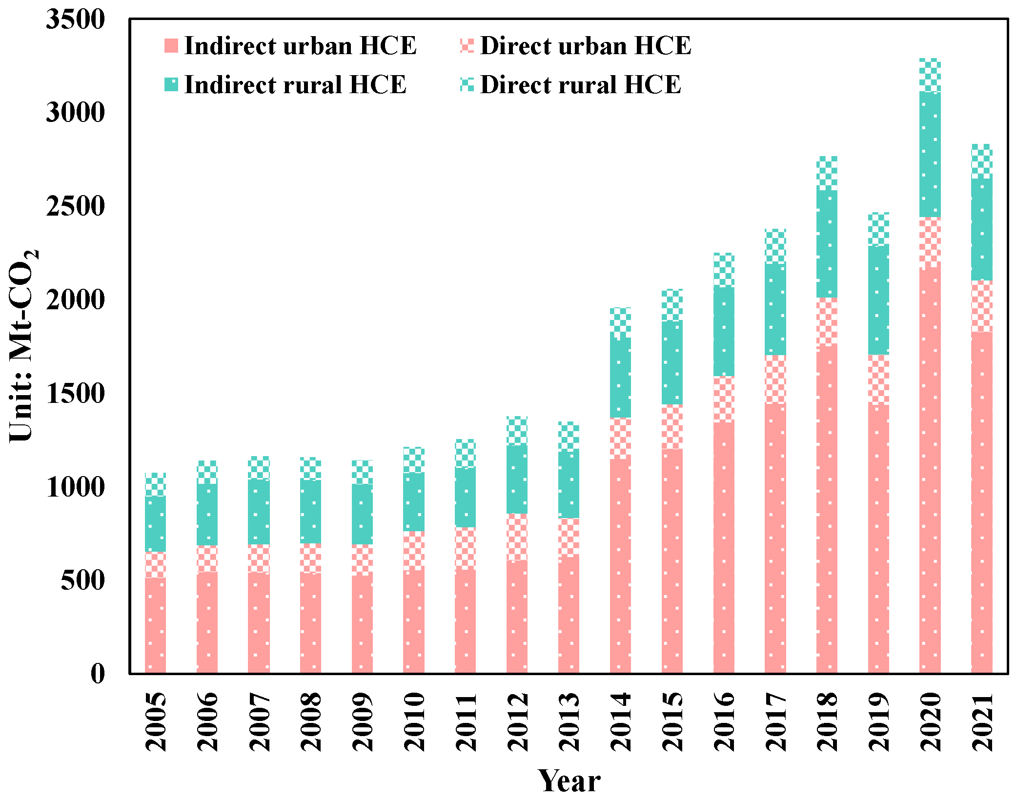
Economic disparities between urban and rural regions are obvious in income levels, lifestyle choices, consumption structures, and other factors [10], leading to significant differences in the CO₂ emissions generated from household consumption. The rapid urbanization in China has fueled income growth and the increasing concentration of energy-intensive sectors in cities, resulting in more carbon-intensive lifestyles among urban households. In 2012, urban households, which made up 53% of the population, were responsible for 75% of national household CO₂ emissions (HCE) [11]. Rural household consumption has also expanded, with rural per capita consumption increasing from 6991 yuan in 2010 to 13,713 yuan in 2020, reflecting a growth rate of 1.96 times. However, rural households exhibit distinct consumption patterns: a higher proportion of their spending goes toward basic needs, and their energy consumption relies more on traditional energy sources.

The emergence of carbon trading is a critical response to the global climate crisis, serving as a key tool for advancing global climate governance and promoting low-carbon development worldwide [12,13]. The fundamental principle of carbon trading involves the transfer of CO₂ emission permits, treated as a scarce resource, thereby raising the cost of emissions and promoting reduction efforts. China began developing its carbon trading market in 2011, launching operations in 2013, and transitioning from regional pilots to a national carbon market in 2021 [14]. Currently, China’s carbon trading market primarily encompasses major emission-intensive sectors, including petrochemicals, chemicals, building materials, steel, and power generation. Carbon trading facilitates reduce emissions in these sectors by optimizing energy use, lowering carbon intensity, and fostering technological innovation [15]. However, when emission costs are incorporated into production costs, businesses often pass a portion of these costs onto consumers. In this way, carbon trading indirectly affects household consumption patterns by influencing the pricing mechanism and the supply–demand dynamics of energy and commodities, ultimately impacting HCE.

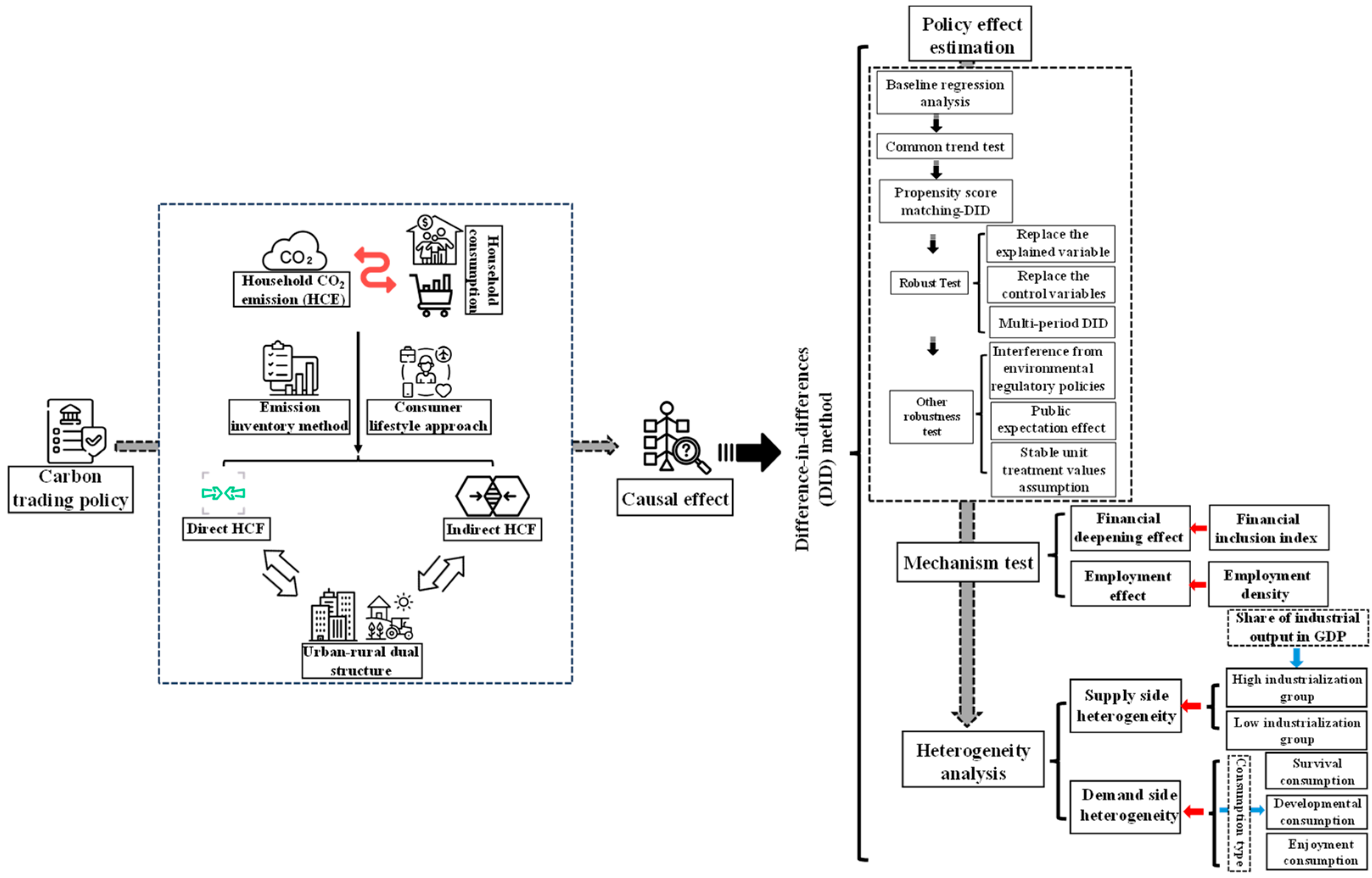
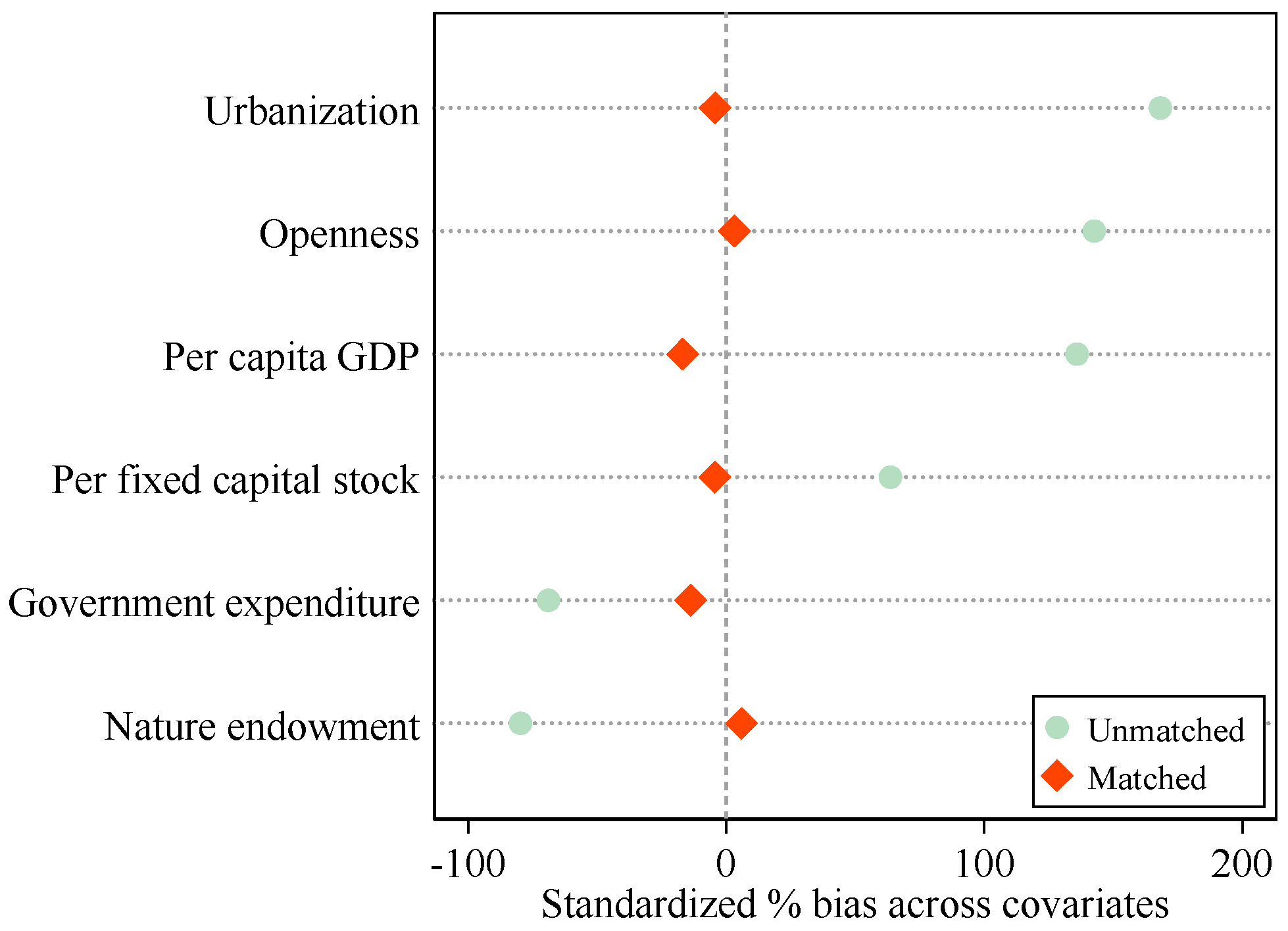
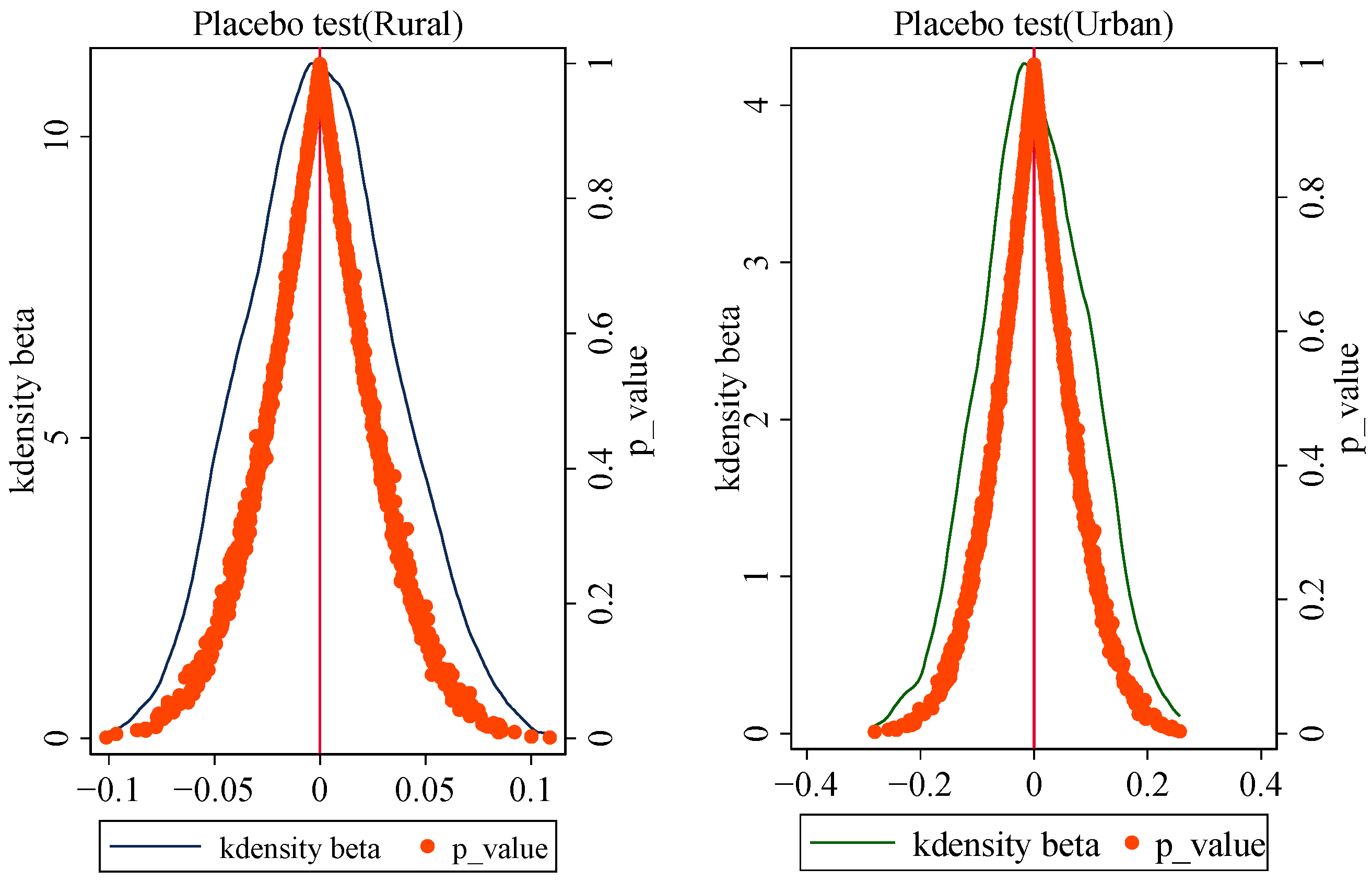
The success of carbon trading policies in lowering high-carbon emissions is vital for meeting China’s dual carbon targets. The purpose of this study is to comprehensively assess the impact of market-oriented environmental policies on HCE from both urban and rural household in China. Using the carbon trading policies introduced in 2013 as a quasi-natural experiment and accurately measuring urban and rural HCE from 2005 to 2021, we employ the difference-in-differences (DID) method to estimate the heterogeneous effects of these policies on HCE. First, utilizing a recalculated provincial HCE dataset that distinguishes between urban and rural areas, we extend the scope of carbon trading policies to the consumption side. Second, we aim to clarify the transmission mechanisms through which carbon trading policies affect HCE, while also investigating the heterogeneity of these effects on the supply side and demand side. Finally, given the potential inequality in policy outcomes caused by China’s urban–rural dual structure, we explore disparities in the effect of carbon trading policies across regions. Understanding the effectiveness of carbon trading policy in mitigating consumption-based emissions can offer fresh insights for the formulation of governmental environmental policies. In addition, by addressing regional carbon inequality, this study contributes to the broader research on equitable carbon reduction strategies.

This study provides multiple marginal contributions to the understanding of sustainable development under China’s dual carbon goals and the field of environmental economics. First, we recalculate the most recent provincial-level CO₂ emission dataset for urban and rural household consumption, identifying and verifying the carbon reduction effect of carbon trading policies on consumption-based emissions. To date, most evaluations of carbon trading policies have focused on production-based emissions, with little attention paid to their impact on the consumption side [16,17]. This study extends the impact boundary of carbon trading policies to the consumption side, significantly enriching and broadening the literature on environmental policy impact assessments. Second, this study reveals the transmission process and mechanisms through which carbon trading policies reduce HCE, examining the heterogeneity of market-based environmental policies on both the supply and demand sides. This provides valuable insights for the government in further broadening the scope of environmental policy. Third, from the perspective of China’s urban–rural dual structure, this study innovatively explores the differences in the intensity of carbon trading policies’ impact on HCE between urban and rural areas. Previous research has mainly focused on the single effect of carbon trading policies, neglecting the potential policy inequality that may arise from urban–rural differences. This study deepens the understanding of carbon trading policies and introduces a new perspective for addressing regional carbon inequality

The structure of this paper is as follows: Section 2 provides a comprehensive review of the relevant literature; Section 3 outlines the empirical strategy and data selection. Section 4 discusses the main findings. Section 5 provides conclusions with policy implications.

2. Literature Review

2.1. Urban and Rural HCE

Economic and demographic factors are widely recognized as having a significant impact on HCE [18]. Among these factors, the urban–rural divide is considered crucial in shaping HCE patterns in China [19,20,21]. Urban and rural areas, as the two primary spatial units of socio-economic development, are often the main basis for analyzing the impact of these influencing factors on CO₂ emissions from household consumption [22,23]. Notably, Cao et al. (2019) and Li et al. (2015) have identified that urban households contribute the majority of CO₂ emissions generated from the consumption side [24,25]. Clarke et al. (2017) further observed that indirect CO₂ emissions caused by the non-energy goods and services were significantly higher than direct CO₂ emissions from energy use [26]. In contrast, the CO₂ emissions of rural household consumption displays distinct characteristics and a substantial scale compared to urban areas [27]. Liu et al. (2023) estimated the rural HCE at the provincial level, finding that housing expenditure and direct CO₂ emissions accounted for 62% of the increase in rural HCE [28]. Moreover, the development gap between urban and rural areas has led to significant disparities in household carbon footprints. Gao et al. (2023) highlighted the inequality in carbon footprints between urban and rural households in China, showing that urban regions tend to exhibit higher carbon and energy footprints, alongside greater inequality, compared to rural regions [29].

2.2. Carbon Trading and Emissions

In the literature on carbon trading policy evaluation, most studies using macro-level data have focused primarily on production-based emissions from enterprises. Both Wang et al. (2022) and Zhang et al. (2020) demonstrated, through theoretical and empirical analyses, that carbon trading policies can effectively mitigate CO₂ emissions, contributing to the goal of carbon neutrality [30,31]. Furthermore, scholars have suggested that carbon trading policies positively affect total factor productivity [32], low-carbon economic growth [33], green innovation [34], poverty alleviation [35], political mobility [16], and carbon market efficiency [12]. Nevertheless, a significant portion of the existing literature on carbon trading has primarily focused on production-based emissions, with limited attention given to consumption-based emissions on the demand side. For example, Chen and Lin (2021) assessed the policy effectiveness of carbon trading on CO₂ emissions during the production process [36]; Yu et al. (2024) evaluated the causal effect of carbon trading schemes on the CO₂ emission efficiency of large thermal power plants in China [37]; and Hu et al. (2024) quantified the effects of emission trading schemes on energy-related CO₂ emissions in China. Their findings consistently suggest that carbon trading significantly enhances carbon and energy performance [38].

2.3. China’s Policies and HCE

While there is limited research directly addressing the impact of carbon trading policies on HCE, existing studies provide valuable insights into how other relevant policies in China influence HCE. This review provides an in-depth analysis of the latest findings in the field. For instance, Wu (2022) estimated the effect of China’s smart city policy on household daily consumption-related CO₂ emissions [39]. Du et al. (2024) examined how the digital economy affect the HCE, using the DID approach as a robustness test [40]. Wei et al. (2024) utilized micro-survey data to evaluate the effect of pro-poor policies on HCE, concluding that such policies effectively mitigate carbon inequality across income groups [41]. Wang et al. (2024) argued that price policies can reduce consumption inequality and lower CO₂ emissions, highlighting the differing effects of these policies across different income brackets and spatial contexts [42]. Moreover, Li et al. (2024) evaluated the effectiveness of China’s carbon inclusion policy, an innovative voluntary emission reduction mechanism, on HCE, showing that the policy significantly lowered HCE [43].

From this review, it is clear that limited attention has been given to the impact of carbon trading policies on consumption-based emissions, particularly in the context of the urban–rural dual structure in China. This research aims to address this gap by investigating the differential impacts of a market-oriented environmental policy—carbon trading—on HCE in urban and rural settings. In doing so, we not only explore the policy’s effectiveness in mitigating carbon emissions but also examine the transmission mechanisms through which these policies affect households in varying socio-economic contexts. By focusing on the urban–rural divide, we contribute to the growing discourse on carbon inequality, shedding light on how environmental policies can both mitigate and exacerbate existing socio-economic disparities. The schematic diagram of this study is as follows (Figure 1).

3. Methodology and Data

Leveraging household consumption data, we first recalculated HCE across all provincial administrative units. Subsequently, employing the DID approach, we evaluated the heterogeneous impacts of carbon trading policies on HCE, with a particular focus on rural–urban disparities.

3.1. The Estimation of HCE

HCE can be divided into two distinct categories: direct and indirect. Direct HCE is generated from energy consumption activities within households, such as cooking and space heating. Indirect HCE, on the other hand, originates from non-energy consumption, where the associated CO₂ emissions occur during the production stages rather than during their use. Accordingly, we have conducted separate estimations for direct and indirect HCE.

3.1.1. Direct HCE by Emission Inventory Method

The fundamental principle of the emission inventory method is that the CO₂ emissions generated by a certain energy source are primarily determined by the emission levels (e.g., energy consumption amount) and emissions coefficients [44]. Most studies typically follow the emission inventory method recommended by the Intergovernmental Panel on Climate Change (IPCC) in the 2006 National Greenhouse Gas Inventory Guidelines to calculate direct HCE.

The formula of emission factor accounting method is as follows:

$${\mathrm{D}\mathrm{I}\mathrm{C}}_{\mathrm{r}}^s=\sum _{i=1}^n{E}_i\times F_i^{s\mathrm{r}}$$

(1)

$${\mathrm{D}\mathrm{I}\mathrm{C}}_{\mathrm{u}}^s=\sum _{i=1}^n{E}_i\times F_i^{s\mathrm{u}}$$

(2)

$$E_i={NCV}_i\times {CC}_i\times {OF}_i\times {\displaystyle \frac{44}{12}}$$

(3)

where ${\mathrm{D}\mathrm{I}\mathrm{C}}_{\mathrm{r}}^s$ and ${\mathrm{D}\mathrm{I}\mathrm{C}}_{\mathrm{u}}^s$ denote the direct HCE of rural and urban areas in $s$ province, respectively; $E_i$ represents the CO₂ emissions coefficient of $i$ energy; $F_i^{s\mathrm{r}}$ and $F_i^{s\mathrm{u}}$ refer to the consumption of energy $i$ in rural and urban areas of $s$ province; ${NCV}_i$ is the low calorific value of energy $i$; ${CC}_i$ is the carbon content per unit calorific value of energy $i$; ${OF}_i$ is the carbon oxidation rate of energy $i$; $i=1\cdots 17$ energy types; $s=1\cdots 30$ provinces. The related information of energy included in household consumption is shown in

Table 1. CO₂ emission coefficients by energy type.

Energy Type	Average Low Calorific Value (KJ/kg; KJ/m3)	Carbon Content (kg-C/GJ)	Oxidation Rate
Raw Coal	20908	25.80	0.94
Cleaned Coal	26344	25.41	0.93
Other Washed Coal	8363	25.41	0.90
Briquettes	15906	33.60	0.90
Coke	28435	29.50	0.93
Coke Oven Gas	16726	12.10	0.99
Other Gas	3763	70.80	0.99
Other Coking Products	34324	29.50	0.93
Crude Oil	41816	20.10	0.98
Gasoline	43070	18.90	0.98
Kerosene	43070	18.90	0.98
Diesel Oil	42652	20.20	0.98
Fuel Oil	41816	21.10	0.99
Liquefied petroleum gas	50179	17.20	0.98
Refinery Gas	45998	15.70	0.98
Other Petroleum Products	37623	20.00	0.98

Note: IPCC guidelines for national GHG emissions inventory.

.

3.1.2. Indirect HCE by the Consumer Lifestyle Approach (CLA)

The core concept of the CLA, as introduced by Bin and Dowlatabadi (2005) [45], involves breaking down all elements of a household’s lifestyle into individual components.

CLA is a consumer-oriented methodology that thoroughly evaluates energy use and CO₂ emissions. It integrates emission coefficients with consumption expenditure to calculate consumption-based emissions. In recent years, this method has been frequently employed to analyze CO₂ emissions associated with household consumption in China [27,40,46].

The China Statistical Yearbook provides comprehensive statistical data on household consumer behavior, organized into eight distinct categories, with each category comprising several related sectors (

Table 2. Household consumption categories and corresponding sectors.

Consumption Categories	Corresponding Industries
Food	Farming, Forestry, Animal Husbandry, Fishery and Water Conservancy; Food Processing; Food Production; Beverage Production
Clothing	Textile Industry; Garments and Other Fiber Products; Leather, Furs, Down, and Related Products
Residence	Construction; Nonmetal Mineral Products; Metal Products; Electric Power, Steam and Hot Water Production and Supply; Gas Production and Supply; Tap Water Production and Supply
Household facilities, articles, and services	Timber Processing, Bamboo, Cane, Palm and Straw Products; Furniture Manufacturing; Rubber and Plastic Products; Electric Equipment and Machinery
Transport and communication services	Transportation Equipment; Electronic and Telecommunications Equipment; Transport, Storage, Postal, and Telecommunications Services
Education, cultural, and recreation services	Papermaking and Paper Products; Printing and Record Medium Reproduction; Cultural, Educational, and Sports Articles
Medicine and medical services	Medical and Pharmaceutical Products
Miscellaneous commodities and services	Tobacco Processing; Wholesale, Retail Trade and Catering Service

). Additionally, this study utilized the average annual household consumption expenditure to calculate indirect HCE. It is important to note that the provincial statistical yearbooks do not further disaggregate the eight categories into sectoral data; thus, this study can only evaluate the indirect HCE in terms of the respective total expenditures on these eight categories. Based on the provincial energy consumption inventory, this study estimated the industrial direct CO₂ emissions across provinces. By integrating these data with the value-added metrics of every economic sector, we subsequently calculated the carbon intensity across consumption classification.

According to the corresponding relationship in Table 2, the indirect HCE from rural and urban household consumption are estimated in the following manner:

$${\mathrm{I}\mathrm{N}\mathrm{C}}_{\mathrm{r}}^s=\sum _j^n({\mathrm{C}\mathrm{I}}_j\times {\mathrm{P}\mathrm{C}\mathrm{E}}_j^{s\mathrm{r}})\times {\mathrm{R}\mathrm{N}}^s$$

(4)

$${\mathrm{I}\mathrm{N}\mathrm{C}}_{\mathrm{u}}^s=\sum _j^n({\mathrm{C}\mathrm{I}}_j\times {\mathrm{P}\mathrm{C}\mathrm{E}}_j^{s\mathrm{u}})\times {\mathrm{U}\mathrm{N}}^s$$

(5)

$${\mathrm{C}\mathrm{I}}_j={\displaystyle \frac{C_j}{V_j}}$$

(6)

where ${\mathrm{I}\mathrm{N}\mathrm{C}}_{\mathrm{r}}^s$ and ${\mathrm{I}\mathrm{N}\mathrm{C}}_{\mathrm{u}}^s$ refer to the indirect HCE, respectively; ${\mathrm{C}\mathrm{I}}_j$ denotes the carbon intensity of the consumption $j$; ${\mathrm{P}\mathrm{C}\mathrm{E}}_j^{s\mathrm{r}}$ and ${\mathrm{P}\mathrm{C}\mathrm{E}}_j^{s\mathrm{u}}$ are the per capita household consumption of category $j$ in rural and urban areas in $s$ province; ${\mathrm{R}\mathrm{N}}^s$ and ${\mathrm{U}\mathrm{N}}^s$ denote the number of rural and urban households in $s$ province; $C_i$ denotes the total CO₂ emissions from industries within category $j$; and $V_j$ represents the aggregate value added by the industries within category $j$.

3.2. Estimation Strategy

3.2.1. DID Approach

Given the widespread application of the DID approach in policy effect evaluation [47,48], we developed a DID model to examine how the carbon trading policy influences HCE. We treat the carbon trading pilot launched in 2013 as an independent “natural experiment”, categorizing the provinces involved in the pilot as the treatment group and those not involved as the control group. The impact of the policy is assessed through the differences in outcomes between these two groups both prior to and following the implementation of the pilot. Additionally, we included several control variables in the model to account for potential “noise” factors, thereby partially alleviating the challenges associated with non-random assignment inherent in quasi-natural experiments.

The standard DID model can be represented in the following estimation form:

$$Y_{st}=\alpha +\beta {treat}_s\ast T_t+\delta {Control}_{st}+{\gamma }_t+{\mu }_s+{\epsilon }_{st}$$

(7)

where $s$ represents the province; $t$ indicates the year; and $Y_{st}$ represents either the rural HCE or the urban HCE. If a province $s$ is part of the carbon trading pilot, then ${treat}_s=1$; otherwise, ${treat}_s=0$. $T_t$ is a dummy variable, where $T_t=1$ indicates all years after the policy implementation, otherwise $T_t=0$. ${Control}_{st}$ is the control variable; $\alpha$ serves as the intercept. ${\mu }_s$ represents the province fixed effects, which account for all time-invariant characteristics that may influence the outcome variable. ${\gamma }_t$ represents the year fixed effects, which control for general shocks that may occur in a specific year; ${\epsilon }_{st}$ is the random error component, characterized by independent and identically distributed properties. After taking the conditional expectation of Equation (7), the coefficient $\beta$ represents the policy effect.

3.2.2. Common Trend Testing and Policy Dynamic Effects

The assumption of common trends is essential for the DID model to accurately identify causal effects. As it is impossible to observe the counterfactual scenarios for the group receiving the treatment after the intervention, researchers often verify the parallel trend assumption indirectly. This is accomplished by analyzing whether the pre-treatment trends of observable variables in both the treated and control groups exhibit a similarity. This study examines the pre-treatment balance trend and the post-treatment dynamic effects by formulating the following equation:

$$\begin{gathered} Y_{st}=\alpha +{\sum }_{p=1}^{T_D-2}{\beta }_p^{pre}{treat}_s\ast T_t^p+{\sum }_{p=T_D}^T{\beta }_p^{post}{treat}_s\ast T_t^p+\delta {Control}_{st}+{\gamma }_t+ \\ {\mu }_s+{\epsilon }_{st} \end{gathered}$$

(8)

where ${treat}_s$ is the treatment indicator variable, and $T_t^p$ represents the time dummy variable for period $p$. ${\beta }_p^{pre}$ and ${\beta }_p^{post}$ can be intuitively understood as the differences in the outcome variable $Y_{st}$ in period $p$. To address potential collinearity issues, this study established the year before the implementation of the carbon trading policy, specifically 2012, as the baseline period. Thus, the validity of pre-treatment parallel trends can be indirectly assessed by testing whether ${\beta }_p^{pre}$ is significantly different from zero. ${\beta }_p^{post}$ represents the policy effects in different periods after the policy implementation and was used to discuss the dynamic effects of the policy.

3.2.3. Propensity Score Matching–Difference in Differences Model (PSM-DID)

While the DID model does not require a similarity between treatment and control groups across all dimensions, non-randomness may arise if certain pre-treatment characteristics related to the outcome variable are imbalanced between these groups. In such cases, the common trend assumption may not serve as effective empirical evidence [49]. To address potential endogeneity issues stemming from selection bias, we utilized the PSM technique to identify appropriate control groups from provinces that did not participate in the pilot study prior to applying the DID model. We choose the logit model to estimate the parameters:

$$P_s=P(s=treat|{Control}_{st})$$

(9)

where ${Control}_{st}$ is a matching variable that can influence the probability of a province being selected into the treatment group. Its definition is consistent with the above. After excluding provinces with matching failure, the treatment group and control group are more likely to align the equilibrium trend assumption, which in turn attenuates bias and ensures the randomness of the policy implementation.

3.2.4. Mechanism Test Model

Accurate identification of conduction mechanisms is difficult in the DID analysis framework. Thus, we draw on the research framework of Chen et al. (2020) [50] to identify the mechanisms through which policies impact HCE. We first find the mechanism variable $M_{st}$ based on the theoretical analysis after which we set up the regression equation:

$$M_{st}=\alpha +\rho {treat}_s\ast T_t+\delta {Control}_{st}+{\gamma }_t+{\mu }_s+{\epsilon }_{st}$$

(10)

We determine whether the conduction mechanism exists by testing the significance of the coefficient $\rho$. To further discuss the different moderating effects of the mechanism variable $M_{st}$ on HCE in rural and urban areas, we establish a combined term that reflects the relationship between the policy and mechanism variables. The regression model is specified as follows:

$$\begin{gathered} Y_{st}=\alpha +\theta {treat}_s\ast T_t\ast M_{st}+\beta {treat}_s\ast T_t+\phi M_{st}+\delta {Control}_{st}+{\gamma }_t+{\mu }_s \\ +{\epsilon }_{st} \end{gathered}$$

(11)

where $\theta$ is the moderating effect that we focused on.

3.3. Variables and Data

3.3.1. Dependent Variables

Our explanatory variable is per capita HCE. Based on the calculations in Section 3.1, we further divide per capita HCE into per capita rural total HCE(RtHCE) and per capita urban total HCE(UtHCE), total direct HCE (TdHCE) and total indirect HCE (TiHCE), and rural indirect HCE (RiHCE) and urban indirect HCE (UiHCE).

3.3.2. Independent Variables

The primary variable of interest is the cross-multiplier variable ${treat}_s\ast T_t$, denoted by $\mathrm{D}\mathrm{I}\mathrm{D}$. If region $s$ implements the carbon trading policies at time $t$, then $\mathrm{D}\mathrm{I}\mathrm{D}=1$; otherwise, $\mathrm{D}\mathrm{I}\mathrm{D}=0$. In this study, the provinces of Beijing, Chongqing, Tianjin, Hubei, Shanghai, and Guangdong are identified as the intervention group, with 2013 set as the year when the policy impact commenced for these pilot regions.

3.3.3. Control Variables

To address potential endogeneity issues and various factors that may simultaneously influence urban and rural HCE, we identified a set of provincial-level control variables that may influence the results of the regression analysis. Drawing on the studies [32,51,52,53,54], we identified six control variables as follows:

• Per capita GDP: Measured by real per capita GDP (2000 constant price).
• Openness: Characterized as the proportion of total imports relative to GDP, serving as an indicator of the region’s trade integration.
• Per capita fixed capital stock: Determined through the perpetual inventory approach for the fixed capital stock in the region (2000 constant price). The assumptions for capital depreciation and growth rates are based on Zhang (2008) [55].
• Government expenditure: Expressed as a percentage of regional fiscal expenditures in relation to GDP.
• Urbanization: Defined as the fraction of the urban population compared to the total population.
• Natural endowment: Measured by the area of nature reserves.

3.3.4. Data

The analysis focused on macroeconomic data from 30 provinces in China for the years during 2005–2021. Due to data limitations, Tibet, Hong Kong, Macao, and Taiwan were excluded from the research. Household consumption data of direct energy were derived from the provincial energy consumption inventory [56] and China Energy Statistical Yearbook [57]. Statistical data concerning consumer behavior were gathered from the provincial yearbooks and reports. Industrial direct energy consumption data came from the provincial energy consumption inventory. The added value of industrial products was taken from China’s industry statistical yearbook [58].

Table 3. Descriptive Statistics.

	Symbol	Variables Definition	Treatment Group (N = 102)		Control Groups (N = 408)
			Mean	S.D.	Mean	S.D.
Explained Variables	RtHCE	Rural total HCE by person	0.996	0.489	1.143	0.824
	UtHCE	Urban total HCE by person	1.537	0.722	2.027	1.425
	TdHCE	Total direct HCE by person	0.897	0.453	0.563	0.288
	TiHCE	Total indirect HCE by person	1.636	0.894	2.606	2.076
	RiHCE	Rural indirect HCE by person	0.523	0.237	0.876	0.703
	UiHCE	Urban indirect HCE by person	1.113	0.682	1.731	1.392
Control Variables	Per capita GDP	Per capita GDP (2000 constant price)	2.164	1.194	0.969	0.346
	Openness	Total goods imports as a percentage of GDP	0.738	0.520	0.186	0.170
	Government expenditure	Government expenditure as a percentage of GDP	0.182	0.040	0.237	0.106
	Urbanization	Urban population as a percentage of the total population	0.737	0.145	0.516	0.102
	Per capita fixed capital stock	Fixed capital stock by person (2000 constant price)	4.337	3.527	3.684	3.282
	Nature endowment	Total area of Nature Reserve	80.657	96.248	426.047	604.049

presents the descriptive statistics for all variables analyzed in the study.

4. Results and Discussion

4.1. Characteristics of HCE Composition

We employed MATLAB 2023a software to estimate provincial-level consumption-based CO₂ emissions in China. The results indicate that HCE in China has exhibited a sustained growth trend from 2005 to 2021, aligning with China’s rapid increase in consumer consumption driven by the continuous expansion of domestic demand (Figure 2). Notably, significant changes in HCE occurred around 2013, 2017, and 2019.

Following 2013, a marked increase in HCE was primarily attributable to the inclusion of imputed rent for self-owned housing in urban household consumption, while the imputed rent for rural households remained zero (

Table 4. Baseline regression analysis for HCE.

Variables	(1)	(2)	(3)	(4)
	RtHCE	UtHCE	TdHCE	TiHCE
DID	−0.477 ***	−0.393 ***	0.023	−0.893 ***
	(0.065)	(0.108)	(0.038)	(0.142)
Time fixed effects	Control	Control	Control	Control
Province fixed effects	Control	Control	Control	Control
Observations	510	510	510	510
R-squared	0.807	0.793	0.847	0.794

Robust standard errors are presented in parentheses. Significance levels are indicated as follows: *** p < 0.01.

). After 2017, however, the growth rate of HCE slowed. This deceleration can be partially explained by the upgrading of household consumption patterns, influenced by the “2018–2020 Implementation Plan for Improving the Consumption Promotion System and Mechanism” [59]. Additionally, the nationwide promotion of carbon trading pilots, which began in 2017, has effectively reflected enterprise-side carbon reductions in HCE through the market circulation of goods. Moreover, urban households account for the majority of total HCE, with indirect HCE significantly exceeding direct HCE in terms of its contribution.

4.2. Policy Effect Estimation

4.2.1. Baseline Regression

We employed Stata 16.0 software to estimate the results of the DID regression. We first assessed the impact of carbon trading policies on reducing CO₂ emissions without incorporating control variables. The regression analysis revealed that the coefficients for rural and urban HCE in relation to the policy variable (DID) were −0.48 and −0.39, respectively. Both coefficients were statistically significant at the 1% level, as shown in Table 4, columns 1 and 2.

We then analyzed the effects from the perspective of direct and indirect HCE. The results revealed that the policy effect on direct HCE was not significant, whereas the regression coefficient for indirect HCE was significantly negative (Table 4, columns 3 and 4). As of 2021, China’s carbon trading market primarily encompassed eight key industries (including petrochemical, chemical, building materials, steel, non-ferrous metal, papermaking, power, and aviation industries). Direct HCEs are mainly associated with sectors that were not fully included in carbon trading policies. For example, the proportion of direct HCE in rural areas is relatively high, predominantly stemming from coal and briquettes. Notably, the coal industry was not included in the early stages of the carbon trading market. Moreover, household energy demand is more sensitive to price factors, which are influenced by the dynamics of energy supply and demand. While carbon trading policies have contributed to optimizing the energy structure of household consumption to some extent, it remains challenging to fully shift household dependence on conventional energy sources in the short term. In contrast, indirect HCEs are determined by the carbon intensity of production across industries, which is more directly impacted by the trading of emission rights under carbon trading policies. Therefore, the estimated policy effects better capture the causal relationship for indirect HCE compared to direct HCE.

Table 5. Baseline regression analysis of indirect HCE.

Variables	(1)	(2)	(3)	(4)
	RiHCE	RiHCE	UiHCE	UiHCE
DID	−0.356 ***	−0.365 ***	−0.537 ***	−0.839 ***
	(0.043)	(0.048)	(0.108)	(0.111)
Government expenditure		2.173 ***		5.055 ***
		(0.632)		(1.255)
Per capita fixed capital stock		−0.072 ***		−0.121 ***
		(0.010)		(0.021)
Openness		−0.546 ***		−1.517 ***
		(0.129)		(0.306)
Per capita GDP		−0.614 ***		−1.291 ***
		(0.123)		(0.259)
Urbanization		0.116		−3.600 **
		(0.623)		(1.463)
Nature endowment		−0.002 ***		−0.004 ***
		(0.001)		(0.001)
Time fixed effects	Control	Control	Control	Control
Province fixed effects	Control	Control	Control	Control
Observations	510	510	510	510
R-squared	0.793	0.839	0.783	0.838

Robust standard errors are presented in parentheses. Significance levels are indicated as follows: *** p < 0.01, ** p < 0.05.

illustrates the impact of carbon trading policies on indirect HCE. The regression results in columns 1 and 3 are estimated without control variables, incorporating only fixed effects for time and province. The results indicate that carbon trading policies have a substantial impact in reducing indirect HCE, with the effect being statistically significant at the 1% level. Incorporating control variables, columns 2 and 4 provide further evidence that the regression coefficients remain negative and, thus, emphasizes the clear urban–rural disparities. For instance, the carbon reduction effect is more pronounced for households in urban areas (−0.839) compared to those in rural areas (−0.365).

Generally, per capita GDP, openness, per capita fixed capital stock, and natural endowment all exhibit significant negative effects on indirect HCE. The impact of urbanization on rural HCE is insignificant; however, it plays a notable role in curbing HCE growth in urban areas. In regions with higher rates of urbanization, urban development tends to prioritize ecological sustainability. Additionally, in areas with higher government expenditure, household income can increase through transfer payments, which may ultimately drive higher HCE.

4.2.2. Common Trend Test Results

To assess whether changes in HCE in the provinces subjected to carbon trading policies can be attributed to these policies and to account for the influence of other factors, we conducted a common trend test to compare HCE before and after the implementation of these policies (Figure 3). Before the implementation of carbon trading, no significant difference in HCE existed between the treatment and control provinces in both urban and rural areas, thereby confirming the validity of the common trend assumption. After the implementation of the carbon trading market, the policy’s carbon reduction effects became increasingly evident, with a more pronounced impact in urban regions. In addition, the urban policy effect showed fluctuations after the third period, whereas in rural areas, it weakened after the seventh period. The findings indicate that, over the long term, the policy fosters the transition to low-carbon lifestyles, with urban areas adopting low-carbon concepts at an earlier stage compared to rural areas.

4.2.3. PSM-DID Results

To account for potential non-random effects of carbon trading policies and to ensure comparability between the treatment and control groups, we employed the PSM-DID method as a robustness check. We treated the control variables as matching covariates and employed a logit regression model to calculate the propensity scores. Subsequently, we performed a matching procedure with a 1:4 ratio using the nearest neighbor approach [60]. Prior to matching, there were substantial discrepancies between the treatment and control groups, with some variables showing deviations exceeding 100%. After matching, the deviation of each covariate between the two groups was significantly reduced, falling within an acceptable range, which indicates satisfactory matching quality (Figure 4). We then excluded groups with poor matching quality and re-estimated the regression equation. The results confirm that our baseline findings remain robust (

Table 6. Estimation outcomes of PSM-DID.

Variables	(1)	(2)
	RiHCE	UiHCE
DID	−0.381 ***	−0.827 ***
	(0.062)	(0.114)
Control variables	Control	Control
Time fixed effects	Control	Control
Province fixed effects	Control	Control
Observations	277	277
R-squared	0.915	0.907

Robust standard errors are presented in parentheses. Significance levels are indicated as follows: *** p < 0.01.

).

4.2.4. Replacement of Dependent Variables, Control Variables, and Estimation Methods

The methodology for calculating housing expenditure within household consumption underwent changes in 2013. In order to address the potential influence of this change on our analysis, CO₂ emissions related to housing were excluded from total HCE, and we used this adjusted HCE as the dependent variable in our analysis. The findings indicate that carbon trading policies still significantly reduced HCE (

Table 7. Robustness test—replacement of dependent variables, control variables and estimation methods.

Variables	Replacement of Dependent Variables		Time-Invariant Control		Multi-Point DID
	(1)	(2)	(3)	(4)	(5)	(6)
	RiHCE	UiHCE	RiHCE	UiHCE	RiHCE	UiHCE
DID	−0.077 ***	−0.154 ***	−0.318 ***	−0.833 ***
	(0.013)	(0.028)	(0.047)	(0.106)
DID_M					−0.368 ***	−0.776 ***
					(0.046)	(0.103)
${Control}_{s,2005}\ast year$			Control	Control
Control variables	Control	Control			Control	Control
Time fixed effects	Control	Control	Control	Control	Control	Control
Province fixed effects	Control	Control	Control	Control	Control	Control
Observations	510	510	510	510	510	510
R-squared	0.806	0.811	0.827	0.815	0.842	0.841

Robust standard errors are presented in parentheses. Significance levels are indicated as follows: *** p < 0.01.

, columns 1 and 2), indicating that the changes in statistical methodology did not affect the key attributes of HCE.

Variables which change post-treatment are likely influenced by the policy, making them potential ‘bad’ control variables. Following Cinelli et al. (2022) [61], we selected 2005 as the base period and incorporated deterministic time trends by multiplying all control variables by the year (${Control}_{s,2005}\ast year$). This approach assessed the robustness of the variables employed in the benchmark analysis. The results demonstrate that policy effects remain significantly negative (Table 7, columns 3 and 4).

Since China established carbon exchanges in Fujian and Sichuan provinces in 2016, we included these provinces as treatment groups in our regression model. We employed a multi-period DID estimation method and introduced a new policy variable (DID_M). The regression results show that the policy effects remain robust across different specifications (Table 7, columns 5 and 6).

4.2.5. Other Robustness Test Results

To ensure that the experimental conclusions of this study were not influenced by unobservable factors, we randomly selected six provinces from the sample to form a virtual experimental group and conducted a Monte Carlo test, repeating the process 1000 times to generate the distribution of kernel density of the primary explanatory variables (Figure 5). Additionally, to further mitigate potential interference from other environmental regulations, for example, the emissions trading policy (ETP) and the low-emission urban initiative (LEU), we have incorporated the aforementioned policy impacts into Equation (7). The coefficients of the key policy variables of interest remained significantly negative (

Table 8. Robustness test—competitive policy, expected effect, and spillover effect.

Variables	Competitive Policy Test		Expected Effect Test		Spillover Effect Test
	(1)	(2)	(3)	(4)	(5)	(6)	(7)	(8)
	RiHCE	UiHCE	RiHCE	UiHCE	RiHCE	UiHCE	RiHCE	UiHCE
DID	−0.341 ***	−0.817 ***	−0.265 ***	−0.731 ***			−0.537 ***	−1.187 ***
	(0.052)	(0.119)	(0.087)	(0.222)			(0.066)	(0.156)
ETP	0.186 **	0.301 **
	(0.091)	(0.162)
LEU	−0.112 **	−0.118
	(0.051)	(0.102)
DID_Pre1			−0.120	−0.129
			(0.090)	(0.267)
DID_Pre2			−0.040	−0.068
			(0.067)	(0.185)
Spillover					−0.348 ***	−0.746 ***
					(0.055)	(0.106)
Control variables	Control	Control	Control	Control	Control	Control	Control	Control
Time fixed effects	Control	Control	Control	Control	Control	Control	Control	Control
Province fixed effects	Control	Control	Control	Control	Control	Control	Control	Control
Observations	510	510	510	510	408	408	289	289
R-squared	0.842	0.840	0.839	0.839	0.857	0.867	0.845	0.844

Robust standard errors are presented in parentheses. Significance levels are indicated as follows: *** p < 0.01, ** p < 0.05. Columns (1) and (2) added (ETP) (LEU) two policies as control variables for regression. Expected effects were added in columns (3) and (4). In column (5), a spillover variable at the provincial level was constructed, that is, the region adjacent to the pilot province is assigned a value of 1, otherwise it is 0. After excluding the pilot province, the spillover effect was estimated. In column 6, the provinces adjacent to the pilot provinces were excluded, and then the regression was carried out.

, columns 1 and 2).

Although the carbon trading policies were formally implemented in 2013, relevant documents had been issued as early as 2011. To account for potential anticipatory effects formed prior to the carbon trading policy rollout, we constructed policy variables for the year before the pilot (DID_Pre1) and two years prior (DID_Pre2) and included them in Equation (1). The coefficient for these proxy variables of anticipatory effects was not statistically significant (Table 8, columns 3 and 4), indicating that the carbon trading policies were not affected by such anticipatory behavior.

In principle, the treatment and control groups should remain strictly separate. However, if the treatment group benefits from more favorable policies, individuals from the control group may migrate to treatment areas, resulting in spillover effects. Drawing on existing research [62,63], we found evidence of a spillover effect from the carbon trading policies (Table 8, columns 5 and 6). To mitigate this effect, we excluded provinces neighboring the pilot provinces and re-ran the regression analysis. The results show that the policy variables remained negative at the 1% significance level (Table 8, columns 7 and 8).

4.3. Mechanism Test

4.3.1. Financial Deepening Effect

Financial deepening can significantly influence household consumption behavior, thereby affecting HCE [64,65]. Moreover, the goods consumed by households are produced in the supply sector, and previous literature suggests that financial deepening is a key determinant of production-based emissions [66,67,68,69]. Since carbon trading essentially operates as a financial market [13], financial deepening can be viewed as a beneficial complement to carbon trading policies [70].

We used the financial inclusion index (FII), developed by Peking University, as a proxy variable to assess the impact of financial deepening (

Table 9. Financial deepening effect.

Variables	(1)	(2)	(3)
	FII	RiHCE	UiHCE
DID	0.045 **	0.143	−0.087
	(0.022)	(0.119)	(0.319)
FII_DID		−0.157 ***	−0.225 **
		(0.038)	(0.089)
Control variables	Control	Control	Control
Time fixed effects	Control	Control	Control
Province fixed effects	Control	Control	Control
Observations	330	330	330
R-squared	0.997	0.915	0.893

Robust standard errors are presented in parentheses. Significance levels are indicated as follows: *** p < 0.01, ** p < 0.05. Since the inclusive finance index compiled by Peking University covers the period from 2011 to 2021, the number of samples in columns 1 and 3 is 330.

). The regression coefficient of the FII with respect to the DID policy indicator is significant at the 5% level, suggesting that carbon trading policies have played a role in promoting regional financial deepening. This finding implies the presence of potential transmission mechanisms. In addition, the significantly negative coefficient of the interaction term indicates that financial deepening strengthens the effectiveness of carbon trading policies in reducing emissions. Specifically, regulatory effect on urban households is −0.23, which is higher than the effect on rural households (−0.15). These differences in regulatory impact can be explained from both supply and demand perspectives.

On the supply side, with ongoing financial deepening, social capital increasingly flows into sectors such as environmental protection, energy conservation, and clean energy, gradually lowering the carbon intensity of products. On the demand side, financial deepening primarily affects household consumption behavior.

4.3.2. Employment Effect

Under the influence of social constraints on environmentally harmful public behavior, carbon trading has led to an increase in labor demand in pilot provinces [71,72]. This, in turn, affects household consumption patterns related to transportation, heating, air conditioning, and other goods and services, thereby influencing HCE [73]. Carbon trading facilitates the movement of workers from underdeveloped areas to regions implementing pilot programs and transforms the employment composition of firms involved in the carbon market, particularly by increasing the share of highly skilled workers [74].

To verify the transmission mechanism of the employment effect, we use employment density (ED) as a proxy variable (

Table 10. Employment effect.

Variables	(1)	(2)	(3)
	ED	RiHCE	UiHCE
DID	0.007 ***	−0.401 ***	−1.166 ***
	(0.001)	(0.062)	(0.128)
ED_DID		0.268	5.411 ***
		(1.334)	(2.004)
Control variables	Control	Control	Control
Time fixed effects	Control	Control	Control
Province fixed effects	Control	Control	Control
Observations	510	510	510
R-squared	0.987	0.839	0.844

Robust standard errors are presented in parentheses. Significance levels are indicated as follows: *** p < 0.01.

). The results of dependent variable ED demonstrate a statistically significant impact at the 1% level, this suggests that the implementation of carbon trading policies has led to an increase in regional employment density, providing evidence for the presence of an employment effect. The results for the interaction term (ED_DID) show that the employment effect is significant only in urban areas, which in turn diminishes the effectiveness of carbon trading policies in reducing emissions. More specifically, adoption of these policies has led to increased technical requirements for labor in low-carbon industries [75], which has hindered the employment prospects of low-skilled rural labor.

4.4. Heterogeneity Analysis

4.4.1. Supply Side Heterogeneity Analysis Results

The industrialization level can influence the carbon intensity of consumer goods. China, being a vast country with varying levels of industrial development across its regions, experiences differing impacts from the high-carbon characteristics of industry on the CO₂ emissions associated with regional residents’ consumption behavior. Therefore, this study examined the heterogeneous impacts of the supply side on carbon trading policies by utilizing data on the share of industrial output in relation to the gross regional product during the year of policy implementation. The sample was classified into two groups based on industrialization level, with the 50th percentile serving as the cutoff point (Figure 6).

Overall, carbon trading policies exhibit a significant negative impact in both high- and low-industrialization groups. However, the negative impact is more pronounced in the low-industrialization group compared to the high-industrialization group (

Table 11. Supply side heterogeneity results.

Variables	High Industrialization Level		Low Industrialization Level
	(1)	(2)	(3)	(4)
	RiHCE	UiHCE	RiHCE	UiHCE
DID	−0.176 ***	−0.457 ***	−0.591 ***	−1.117 ***
	(0.041)	(0.087)	(0.182)	(0.386)
Control variables	Control	Control	Control	Control
Time fixed effects	Control	Control	Control	Control
Province fixed effects	Control	Control	Control	Control
Observations	255	255	255	255
R-squared	0.903	0.921	0.841	0.837

Robust standard errors are presented in parentheses. Significance levels are indicated as follows: *** p < 0.01.

). High-industrialization groups have established a robust industrial base, with relatively advanced technology and higher energy efficiency. Most enterprises in these regions have implemented energy-saving and emission reduction measures, thus limiting the marginal impact of carbon trading policies. In contrast, low-industrialization groups have weaker industrial foundations and lower technological levels. The implementation of carbon trading policies provides a greater incentive for enterprises to improve energy efficiency and reduce CO₂ emissions. Therefore, the negative impact of carbon trading policies on HCE is more significant in low-industrialization groups. Additionally, from the perspective of energy structure, high-industrialization groups tend to have more diversified energy sources, with a higher proportion of clean energy usage. In contrast, low-industrialization groups have a relatively homogeneous energy structure, relying heavily on coal and other high-carbon energy sources, leading to higher carbon intensity.

4.4.2. Demand Side Heterogeneity Analysis Results

The sectoral composition of indirect HCE was categorized into three types based on consumption demand for urban-rural comparison (

Table 12. Demand side heterogeneity analysis.

Variables	Survival		Development		Enjoyment
	(1)	(2)	(3)	(4)	(5)	(6)
	RiHCE	UiHCE	RiHCE	UiHCE	RiHCE	UiHCE
DID	−0.321 ***	−0.768 ***	−0.051 ***	−0.068 **	−0.001	−0.007
	(0.050)	(0.109)	(0.011)	(0.027)	(0.003)	(0.014)
Control variables	Control	Control	Control	Control	Control	Control
Time fixed effects	Control	Control	Control	Control	Control	Control
Province fixed effects	Control	Control	Control	Control	Control	Control
Observations	510	510	510	510	510	510
R-squared	0.811	0.812	0.786	0.788	0.253	0.335

Robust standard errors are presented in parentheses. Significance levels are indicated as follows: *** p < 0.01, ** p < 0.05.

): survival consumption (food, tobacco, alcohol, clothing, and housing), developmental consumption (education, culture, entertainment, transportation, communication, and healthcare), and enjoyment consumption (daily necessities and other services).

Carbon trading policies have been shown to effectively mitigate high-carbon consumption behaviors associated with survival-based consumption. For developmental and enjoyment consumption, households with higher levels of demand tend to more readily adopt low-carbon practices, thereby reducing the economic significance of market-oriented policy interventions.

Carbon trading policies’ impact on the demand side carries significant implications for urban-rural carbon inequality. Broadly, the benefits of carbon reduction are reflected in improved social welfare [76]. However, since the social welfare function of public goods is relatively fixed, we designed an indicator, following the approach of Wei et al. (2024) [41], to measure absolute carbon inequality. This indicator, defined as the difference between urban and rural HCE, was included as an explanatory variable in Equation (7). The regression results are displayed in

Table 13. The analysis of carbon inequality.

Variables	Carbon Inequality
	(1)	(2)	(3)	(4)
	Total	Survival	Development	Enjoyment
DID	−0.468 ***	−0.441 ***	−0.020	−0.002
	(0.077)	(0.082)	(0.019)	(0.003)
Control variables	Control	Control	Control	Control
Time fixed effects	Control	Control	Control	Control
Province fixed effects	Control	Control	Control	Control
Observations	510	510	510	510
R-squared	0.785	0.759	0.758	0.407

Robust standard errors are presented in parentheses. Significance levels are indicated as follows: *** p < 0.01.

.

Carbon trading policies have been shown to efficiently reduce regional carbon inequality, particularly in the area of survival consumption. From the standpoint of allocative efficiency, carbon redistribution facilitated by market-based environmental policies has the potential to mitigate carbon inequality between vulnerable and other population groups, thereby contributing to the reduction in the “environmental justice gap” [76].

5. Discussion

We conducted a comprehensive assessment of the positive impacts of carbon trading policies on HCE in urban and rural areas, addressing a less explored area in the literature. Existing studies have primarily examined the effects of China’s carbon trading pilots in reducing production-based emissions in energy-intensive industries and overall regional CO₂ emissions [17,33,36,77,78] and have demonstrated the positive role of carbon trading policies in reducing emissions based on the Porter hypothesis [37]. However, some scholars argue that the impact of carbon market policies on reducing consumption-based emissions is limited [79]. In contrast, our research confirms the positive effect of carbon trading policies on consumption related emissions and emphasizes the urban-rural disparity. This fairness perspective, grounded in cross-sectional comparisons, is critical [80]. Furthermore, our study captures the more pronounced long-term adjustment effects of these policies on households, revealing the specific ways in which policy intensity evolves over time. Studies on the diminishing effects of carbon taxes or carbon trading systems underscore this point [81]. This long-term perspective provides valuable insights into the broader impacts of carbon trading policies on sustainable development under China’s dual carbon goals.

Previous literature has mainly focused on the direct regulatory effects of carbon trading on industrial output and technological innovation [14,35,37], with limited consideration of how these impacts are transmitted to household consumption behavior. We identified two transmission mechanisms—finance and employment—which are crucial for understanding how carbon trading policies affect HCE. On the supply side, as financial markets deepen, increasing amounts of social capital flow into environmental protection, energy-saving technologies, and clean energy sectors, gradually reducing the carbon intensity of products. On the demand side, financial deepening primarily influences household consumption behavior. Urban households, due to higher levels of education and income, are more inclined toward low-carbon consumption practices [65]. Additionally, housing is closely tied to financial liabilities for Chinese households, which explains why financial deepening has different impacts between urban and rural areas. This paper argues that although carbon trading policies do not directly affect income, their implementation comes at the cost of rural residents’ employment opportunities, as they are more likely to lose jobs. This ultimately leads to environmental inequality, consistent with the literature on whether environmental regulations disproportionately impact traditionally disadvantaged regions [35,75].

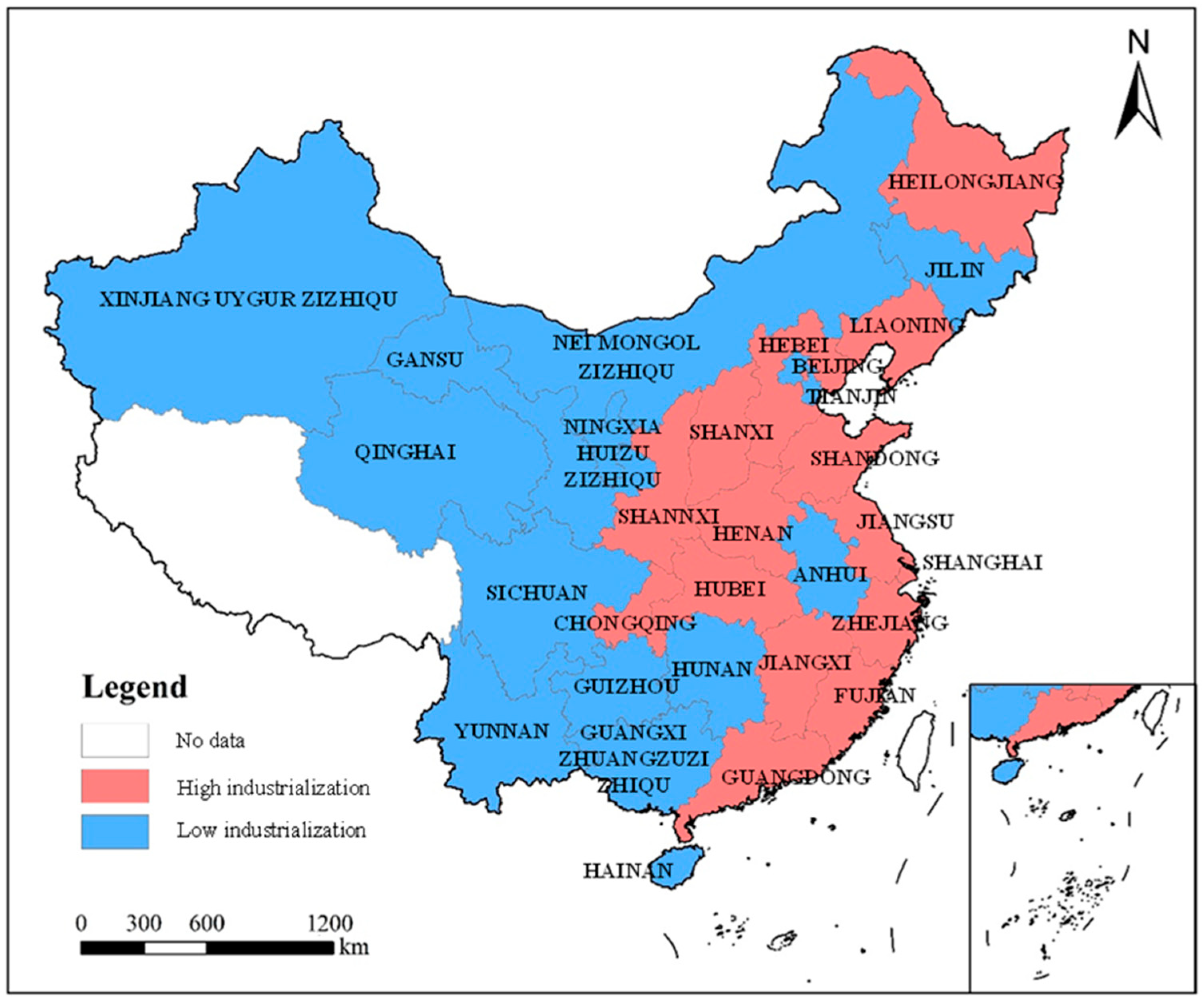
By distinguishing between the supply-side and demand-side effects, we provide a more nuanced understanding of carbon trading policies. The broader literature on carbon markets reveals how regional factors lead to varying policy impacts [33,34]. Our findings offer a more interesting conclusion: highly industrialized regions are more significantly affected by such policies than less industrialized regions. When carbon trading policies encourage both businesses and residents to transition to low-carbon energy, the negative impact on consumption-based emissions is more pronounced among low-industrialization groups. Similarly, this heterogeneity issue also manifests in urban-rural differences. Compared to rural households with lower income elasticity, wealthier urban households respond differently to the price signals of carbon trading [24,42]. These varying responses provide policymakers with more detailed insights, helping them design complementary policies to address the distinct needs and challenges of different regions.

China is committed to improving the urban-rural dual structure, and enhancing the welfare of rural residents is crucial. At the very least, carbon trading policies should not exacerbate their burdens [82]. Research on carbon policies also emphasizes the potential unequal impacts across different regions or socioeconomic groups [83,84]. Unlike much of the literature that holds a pessimistic view of carbon policies, our study confirms the differentiated impacts of market-based policies on the urban-rural dual structure and highlights the positive significance of these policies in reducing carbon inequality. Broadly speaking, understanding residents’ preferences for different types of consumption goods is essential to grasping the role of carbon policies [24,85]. Particularly in areas of subsistence consumption, as income rises, carbon policies can leverage market forces to achieve carbon redistribution, ensuring that the benefits of carbon reduction are considered through an equity lens. This finding provides valuable insights for policymakers seeking to design interventions that not only reduce carbon inequality but also promote carbon reduction.

6. Conclusions and Policy Implication

The implementation of market-oriented environmental policies, such as carbon trading, represents a critical strategy for China in reducing CO₂ emissions and addressing carbon inequality. This study offers an initial exploration of carbon trading policies, with an emphasis on the consumption side. Employing a DID methodology, this study empirically analyzes the heterogeneous impacts of carbon trading policies on HCE, and investigates the underlying mechanisms that explain these variations. The principal outcomes of this research are outlined below:

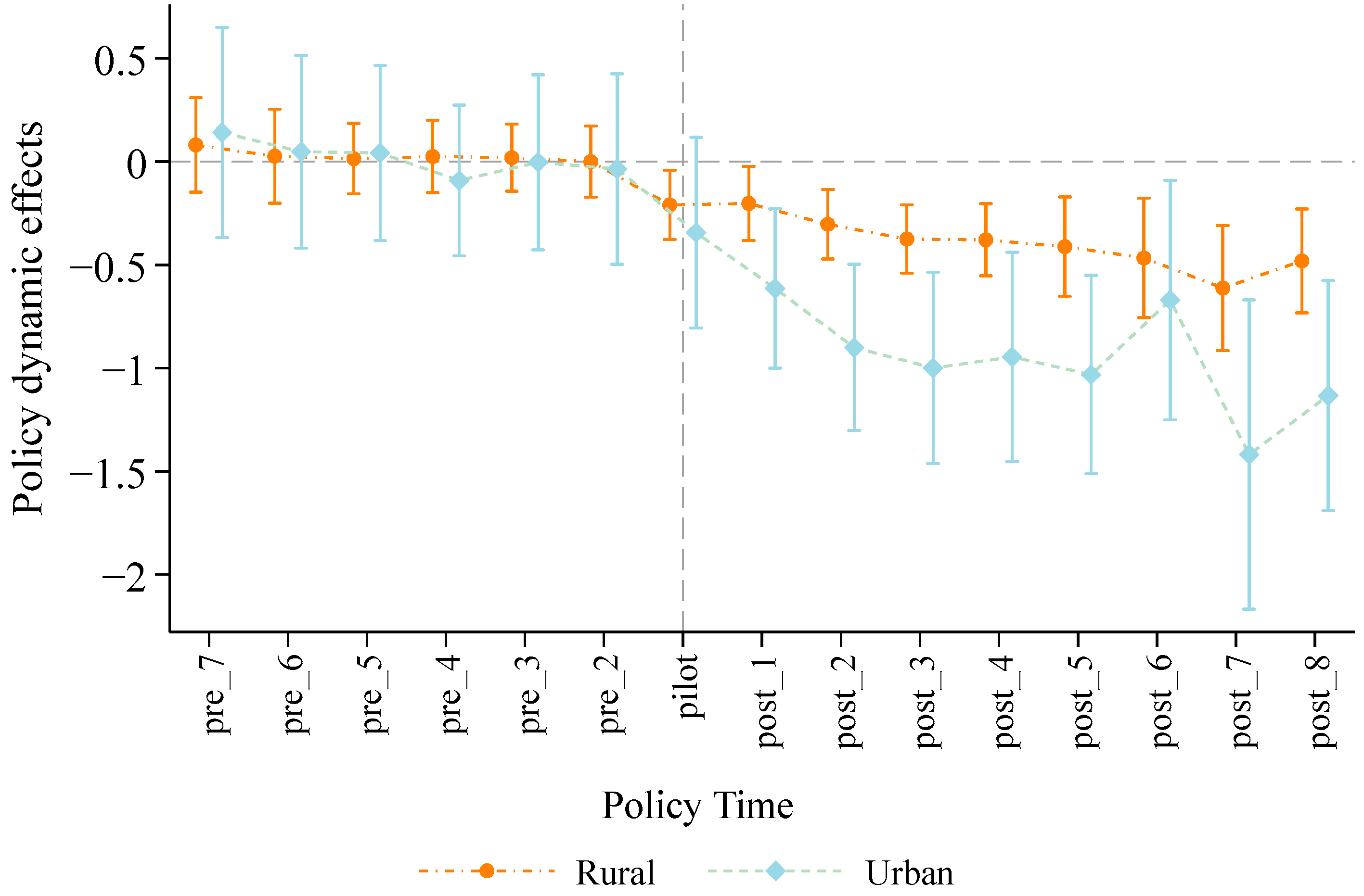
• The implementation of carbon trading policies has led to a notable reduction in HCE, with the most pronounced effects observed in urban areas. Although the policy impact weakened over time, the findings suggest a lasting influence on promoting low-carbon lifestyles among households.
• Financial deepening and employment effects are identified as the primary channels through which the carbon trading market influences HCE. These transmission mechanisms have a more substantial impact on urban households.
• The policy effects differ markedly between urban and rural areas, with carbon trading policies most effectively reducing HCE related to survival consumption, thereby helping to alleviate urban-rural carbon inequality from the demand side.
• In light of the results, the following policy implications are suggested:

First, given the inhibitory effects of carbon trading policies on China’s HCE, policymakers should fully leverage market mechanisms in environmental regulation and further advance market-based incentive policies. Accelerating the establishment of an integrated carbon trading system is crucial for promoting low-carbon lifestyles and supporting China’s objectives of reducing carbon emissions and achieving carbon neutrality.

Second, improving the coordination between carbon trading policies and household consumption is of significant practical importance for alleviating urban-rural carbon inequality. Policymakers should account for the urban-rural dual structure to ensure equitable benefits for rural households. As market-oriented environmental policies may not always promote fair distribution, complementary carbon distribution policies should be designed to prevent the widening of carbon inequality.

Lastly, carbon reduction strategies should be tailored to the cost-effectiveness of household consumption patterns, considering the level of regional industrialization. In highly industrialized regions, regulatory policies should complement market mechanisms to achieve more substantial emissions reductions at lower costs. In less industrialized regions, the application of market-based environmental policies should be expanded to promote cost-effective carbon reduction. Furthermore, policies should target high-carbon products related to household subsistence consumption, adapting to regional variations in consumption needs.

7. Limitations and Future Perspectives

Although one of the study objectives was to explore the impact of China’s carbon trading policy on consumption-based emissions, we acknowledge that there is scope for more precise measurement of HCE. Given that a key focus of our research is to examine changes in the structure of HCE across different provinces in China, we chose the CLA to estimate indirect CO₂ emissions based on annual household consumption data. This method allows us to capture the structural dynamics of consumption emissions over time at the provincial level, which is essential for our analysis. However, this method, admittedly, does not account for the influence of factors such as technological conditions of production and supply chain structures on HCE. In future research, we will attempt to expand the scope of our CO₂ emission estimations, such as environmental extended input–output analysis framework. Moreover, this study focused on China’s provincial-level administrative units, which limits the overall sample size. In future work, we aim to extend the geographical scope to include city-level administrative units across China, which will ensure a more robust and diverse sample for analysis.

Last but not least, during the review process, we received constructive feedback from reviewers, and based on these valuable comments, we made several modifications to improve the study’s clarity and depth. First, we have added a detailed introduction to HCE in the background section to provide a more comprehensive research context. Second, we restructured the introduction to outline the research framework more effectively. Third, we reorganized the literature review to reflect a more thorough understanding of prior work. Lastly, we expanded the discussion of key findings to offer additional insights into the study’s implications. These improvements significantly enhance the study’s contribution to the field and address the reviewers’ valuable suggestions.

References

1. Peters, G.P. From production-based to consumption-based national emission inventories. Ecol. Econ. 2008, 65, 13–23. [Google Scholar] [CrossRef]
2. Wei, Y.-M.; Liu, L.-C.; Fan, Y.; Wu, G. The impact of lifestyle on energy use and CO2 emission: An empirical analysis of China’s residents. Energy Policy 2007, 35, 247–257. [Google Scholar] [CrossRef]
3. Ma, M.; Ma, X.; Cai, W.; Cai, W. Carbon-dioxide mitigation in the residential building sector: A household scale-based assessment. Energy Convers. Manag. 2019, 198, 111915. [Google Scholar] [CrossRef]
4. Liang, Y.; Cai, W.; Ma, M. Carbon dioxide intensity and income level in the Chinese megacities’ residential building sector: Decomposition and decoupling analyses. Sci. Total Environ. 2019, 677, 315–327. [Google Scholar] [CrossRef]
5. Zhou, N.; Khanna, N.; Feng, W.; Ke, J.; Levine, M. Scenarios of energy efficiency and CO2 emissions reduction potential in the buildings sector in China to year 2050. Nat. Energy 2018, 3, 978–984. [Google Scholar] [CrossRef]
6. Cha, M.-K.; Struthers, C.L.; Brown, M.A.; Kale, S.; Chapman, O. Toward residential decarbonization: Analyzing social-psychological drivers of household co-adoption of rooftop solar, electric vehicles, and efficient HVAC systems in Georgia, US. Renew. Energy 2024, 226, 120382. [Google Scholar] [CrossRef]
7. Es-sakali, N.; Zoubir, Z.; Kaitouni, S.I.; Mghazli, M.O.; Cherkaoui, M.; Pfafferott, J. Advanced predictive maintenance and fault diagnosis strategy for enhanced HVAC efficiency in buildings. Appl. Therm. Eng. 2024, 254, 123910. [Google Scholar] [CrossRef]
8. Chen, Z.; O’Neill, Z.; Wen, J.; Pradhan, O.; Yang, T.; Lu, X.; Lin, G.; Miyata, S.; Lee, S.; Shen, C. A review of data-driven fault detection and diagnostics for building HVAC systems. Appl. Energy 2023, 339, 121030. [Google Scholar] [CrossRef]
9. Cai, T.; Li, Y.; Wang, P.; Huang, G.; Liu, J. A Taguchi-STIRPAT input-output model for unveiling the pathways of reducing household carbon emissions under dual-carbon target—A case study of Fujian province. Environ. Sci. Pollut. Res. 2024, 31, 15424–15442. [Google Scholar] [CrossRef]
10. Cao, H.; Chen, C.; Chen, J.; Song, W.; He, J.; Liu, C. Differentiation of urban-rural interface and its driving mechanism: A case study of Nanjing, China. Land Use Policy 2024, 140, 107090. [Google Scholar] [CrossRef]
11. Wiedenhofer, D.; Guan, D.; Liu, Z.; Meng, J.; Zhang, N.; Wei, Y.-M. Unequal household carbon footprints in China. Nat. Clim. Change 2017, 7, 75–80. [Google Scholar] [CrossRef]
12. Zhang, W.; Li, J.; Li, G.; Guo, S. Emission reduction effect and carbon market efficiency of carbon emissions trading policy in China. Energy 2020, 196, 117117. [Google Scholar] [CrossRef]
13. Liu, L.; Chen, C.; Zhao, Y.; Zhao, E. China’s carbon-emissions trading: Overview, challenges and future. Renew. Sustain. Energy Rev. 2015, 49, 254–266. [Google Scholar] [CrossRef]
14. Zhong, J.; Zhang, J.; Fu, M. Does the Carbon Emissions Trading Pilot Policy Have a Demonstrated Impact on Advancing Low-Carbon Technology? Evidence from a Case Study in Beijing, China. Land 2024, 13, 1276. [Google Scholar] [CrossRef]
15. Tang, Y.; Yang, Y.; Xu, H. The impact of China carbon emission trading system on land use transition: A macroscopic economic perspective. Land 2021, 11, 41. [Google Scholar] [CrossRef]
16. Li, Z.; Liu, B. Understanding Carbon Emissions Reduction in China: Perspectives of Political Mobility. Land 2023, 12, 903. [Google Scholar] [CrossRef]
17. Chen, G.; Hu, Z.; Xiang, S.; Xu, A. The Impact of Carbon Emissions Trading on the Total Factor Productivity of China’s Electric Power Enterprises—An Empirical Analysis Based on the Differences-in-Differences Model. Sustainability 2024, 16, 2832. [Google Scholar] [CrossRef]
18. Li, K.; Li, H.; Wang, Y.; Yang, Z.; Liang, S. Household carbon footprints of age groups in China and socioeconomic influencing factors. Sci. Total Environ. 2024, 923, 171402. [Google Scholar] [CrossRef] [PubMed]
19. Liu, L.-C.; Wu, G.; Wang, J.-N.; Wei, Y.-M. China’s carbon emissions from urban and rural households during 1992–2007. J. Clean. Prod. 2011, 19, 1754–1762. [Google Scholar] [CrossRef]
20. Wang, X.; Chen, S. Urban-rural carbon footprint disparity across China from essential household expenditure: Survey-based analysis, 2010–2014. J. Environ. Manag. 2020, 267, 110570. [Google Scholar] [CrossRef]
21. Liu, G.; Zhang, F. China’s carbon inequality of households: Perspectives of the aging society and urban-rural gaps. Resour. Conserv. Recycl. 2022, 185, 106449. [Google Scholar] [CrossRef]
22. Fan, J.-L.; Liao, H.; Liang, Q.-M.; Tatano, H.; Liu, C.-F.; Wei, Y.-M. Residential carbon emission evolutions in urban-rural divided China: An end-use and behavior analysis. Appl. Energy 2013, 101, 323–332. [Google Scholar] [CrossRef]
23. Wu, S.; Hu, S.; Frazier, A.E.; Hu, Z. China’s urban and rural residential carbon emissions: Past and future scenarios. Resour. Conserv. Recycl. 2023, 190, 106802. [Google Scholar] [CrossRef]
24. Cao, Q.; Kang, W.; Xu, S.; Sajid, M.J.; Cao, M. Estimation and decomposition analysis of carbon emissions from the entire production cycle for Chinese household consumption. J. Environ. Manag. 2019, 247, 525–537. [Google Scholar] [CrossRef]
25. Li, Y.; Zhao, R.; Liu, T.; Zhao, J. Does urbanization lead to more direct and indirect household carbon dioxide emissions? Evidence from China during 1996–2012. J. Clean. Prod. 2015, 102, 103–114. [Google Scholar] [CrossRef]
26. Clarke, J.; Heinonen, J.; Ottelin, J. Emissions in a decarbonised economy? Global lessons from a carbon footprint analysis of Iceland. J. Clean. Prod. 2017, 166, 1175–1186. [Google Scholar] [CrossRef]
27. Chen, C.; Liu, G.; Meng, F.; Hao, Y.; Zhang, Y.; Casazza, M. Energy consumption and carbon footprint accounting of urban and rural residents in Beijing through Consumer Lifestyle Approach. Ecol. Indic. 2019, 98, 575–586. [Google Scholar] [CrossRef]
28. Liu, L.; Xu, L.; Wang, S.; Tian, X. The transition patterns of rural household carbon footprint in China. Resour. Environ. Sustain. 2023, 13, 100122. [Google Scholar] [CrossRef]
29. Gao, X.; Chen, X.; Liu, L.-C. Exploring the determinants of the evolution of urban and rural household carbon footprints inequality in China. Energy Policy 2024, 185, 113955. [Google Scholar] [CrossRef]
30. Wang, X.; Huang, J.; Liu, H. Can China’s carbon trading policy help achieve Carbon Neutrality?—A study of policy effects from the Five-sphere Integrated Plan perspective. J. Environ. Manag. 2022, 305, 114357. [Google Scholar] [CrossRef]
31. Zhang, Y.; Li, S.; Luo, T.; Gao, J. The effect of emission trading policy on carbon emission reduction: Evidence from an integrated study of pilot regions in China. J. Clean. Prod. 2020, 265, 121843. [Google Scholar] [CrossRef]
32. Liu, B.; Ding, C.J.; Hu, J.; Su, Y.; Qin, C. Carbon trading and regional carbon productivity. J. Clean. Prod. 2023, 420, 138395. [Google Scholar] [CrossRef]
33. Gao, M. The impacts of carbon trading policy on China’s low-carbon economy based on county-level perspectives. Energy Policy 2023, 175, 113494. [Google Scholar] [CrossRef]
34. Liu, Y.; Liu, S.; Shao, X.; He, Y. Policy spillover effect and action mechanism for environmental rights trading on green innovation: Evidence from China’s carbon emissions trading policy. Renew. Sustain. Energy Rev. 2022, 153, 111779. [Google Scholar] [CrossRef]
35. Zhang, G.; Zhang, N. The effect of China’s pilot carbon emissions trading schemes on poverty alleviation: A quasi-natural experiment approach. J. Environ. Manag. 2020, 271, 110973. [Google Scholar] [CrossRef]
36. Chen, X.; Lin, B. Towards carbon neutrality by implementing carbon emissions trading scheme: Policy evaluation in China. Energy Policy 2021, 157, 112510. [Google Scholar] [CrossRef]
37. Yu, Y.; Zhang, X.; Liu, Y.; Zhou, T. Carbon emission trading, carbon efficiency, and the Porter hypothesis: Plant-level evidence from China. Energy 2024, 308, 132870. [Google Scholar] [CrossRef]
38. Hu, Y.; Ren, S.; Wang, Y.; Chen, X. Can carbon emission trading scheme achieve energy conservation and emission reduction? Evidence from the industrial sector in China. Energy Econ. 2020, 85, 104590. [Google Scholar] [CrossRef]
39. Wu, S. Smart cities and urban household carbon emissions: A perspective on smart city development policy in China. J. Clean. Prod. 2022, 373, 133877. [Google Scholar] [CrossRef]
40. Du, Z.; Xu, J.; Lin, B. What does the digital economy bring to household carbon emissions?—From the perspective of energy intensity. Appl. Energy 2024, 370, 123613. [Google Scholar] [CrossRef]
41. Wei, X.; Li, H.; Wang, Y.; Wei, Q. Impact assessment of poverty alleviation on carbon inequality: Evidence from households in China. J. Clean. Prod. 2024, 450, 141843. [Google Scholar] [CrossRef]
42. Wang, C.; Wang, R.; Fei, X.; Li, L. Price effects of residents’ consumption carbon emissions: Evidence from rural and urban China. Energy Econ. 2024, 135, 107662. [Google Scholar] [CrossRef]
43. Li, R.; Fang, D.; Xu, J. Does China’s carbon inclusion policy promote household carbon emissions reduction? Theoretical mechanisms and empirical evidence. Energy Econ. 2024, 132, 107462. [Google Scholar] [CrossRef]
44. Arioli, M.S.; Márcio de Almeida, D.A.; Amaral, F.G.; Cybis, H.B.B. The evolution of city-scale GHG emissions inventory methods: A systematic review. Environ. Impact Assess. Rev. 2020, 80, 106316. [Google Scholar] [CrossRef]
45. Bin, S.; Dowlatabadi, H. Consumer lifestyle approach to US energy use and the related CO2 emissions. Energy Policy 2005, 33, 197–208. [Google Scholar] [CrossRef]
46. Wang, Z.; Yang, L. Indirect carbon emissions in household consumption: Evidence from the urban and rural area in China. J. Clean. Prod. 2014, 78, 94–103. [Google Scholar] [CrossRef]
47. Angrist, J.D.; Pischke, J.-S. Mostly Harmless Econometrics: An Empiricist’s Companion; Princeton University Press: Princeton, NJ, USA, 2009. [Google Scholar]
48. Semykina, A.; Wooldridge, J.M. Estimating panel data models in the presence of endogeneity and selection. J. Econom. 2010, 157, 375–380. [Google Scholar] [CrossRef]
49. Roth, J.; Sant’Anna, P.H.; Bilinski, A.; Poe, J. What’s trending in difference-in-differences? A synthesis of the recent econometrics literature. J. Econom. 2023, 235, 2218–2244. [Google Scholar] [CrossRef]
50. Chen, Y.; Fan, Z.; Gu, X.; Zhou, L.-A. Arrival of young talent: The send-down movement and rural education in China. Am. Econ. Rev. 2020, 110, 3393–3430. [Google Scholar] [CrossRef]
51. He, X.; Adebayo, T.S.; Kirikkaleli, D.; Umar, M. Consumption-based carbon emissions in Mexico: An analysis using the dual adjustment approach. Sustain. Prod. Consum. 2021, 27, 947–957. [Google Scholar] [CrossRef]
52. Lian, Y.; Lin, X.; Luo, H.; Zhang, J.; Sun, X. Distribution characteristics and influencing factors of household consumption carbon emissions in China from a spatial perspective. J. Environ. Manag. 2024, 351, 119564. [Google Scholar] [CrossRef] [PubMed]
53. Meng, B.; Liu, Y.; Gao, Y.; Li, M.; Wang, Z.; Xue, J.; Andrew, R.; Feng, K.; Qi, Y.; Sun, Y. Developing countries’ responsibilities for CO2 emissions in value chains are larger and growing faster than those of developed countries. One Earth 2023, 6, 167–181. [Google Scholar] [CrossRef]
54. Qiao, W.; Huang, X. Assessment the urbanization sustainability and its driving factors in Chinese urban agglomerations: An urban land expansion-Urban population dynamics perspective. J. Clean. Prod. 2024, 449, 141562. [Google Scholar] [CrossRef]
55. Zhang, J. Estimation of China’s provincial capital stock (1952–2004) with applications. J. Chin. Econ. Bus. Stud. 2008, 6, 177–196. [Google Scholar] [CrossRef]
56. Carbon Emission Accounts and Datasets Provincial Energy Consumption Inventory. Available online: https://www.ceads.net.cn/data/province/ (accessed on 22 July 2024).
57. National Bureau of Statistics China Energy Statistical Yearbook. Available online: https://www.stats.gov.cn/zs/tjwh/tjkw/tjzl/202302/t20230215_1907928.html (accessed on 22 July 2024).
58. National Bureau of Statistics China’s Industry Statistical Yearbook. Available online: https://www.stats.gov.cn/zs/tjwh/tjkw/tjzl/202302/t20230220_1913735.html (accessed on 22 July 2024).
59. General Office of the State Council 2018–2020 Implementation Plan for Improving the Consumption Promotion System and Mechanism. Available online: https://www.gov.cn/gongbao/content/2018/content_5335367.htm (accessed on 15 July 2024).
60. Abadie, A.; Drukker, D.; Herr, J.L.; Imbens, G.W. Implementing matching estimators for average treatment effects in Stata. Stata J. 2004, 4, 290–311. [Google Scholar] [CrossRef]
61. Cinelli, C.; Forney, A.; Pearl, J. A crash course in good and bad controls. Sociol. Methods Res. 2024, 53, 1071–1104. [Google Scholar] [CrossRef]
62. Yu, Y.; Liu, D.; Gong, Y. Target of local economic growth and total factor productivity. Manag. World 2019, 35, 26–42. [Google Scholar]
63. Gao, Y.; Li, M.; Xue, J.; Liu, Y. Evaluation of effectiveness of China’s carbon emissions trading scheme in carbon mitigation. Energy Econ. 2020, 90, 104872. [Google Scholar] [CrossRef]
64. Stephenson, J.; Barton, B.; Carrington, G.; Gnoth, D.; Lawson, R.; Thorsnes, P. Energy cultures: A framework for understanding energy behaviours. Energy Policy 2010, 38, 6120–6129. [Google Scholar] [CrossRef]
65. Han, X.; Wei, C.; Cao, G.-Y. Aging, generational shifts, and energy consumption in urban China. Proc. Natl. Acad. Sci. USA 2022, 119, e2210853119. [Google Scholar] [CrossRef]
66. Khan, M.T.I.; Yaseen, M.R.; Ali, Q. Nexus between financial development, tourism, renewable energy, and greenhouse gas emission in high-income countries: A continent-wise analysis. Energy Econ. 2019, 83, 293–310. [Google Scholar] [CrossRef]
67. Huang, S.; Yang, L.; Yang, C.; Wang, D.; Li, Y. Obscuring effect of income inequality and moderating role of financial literacy in the relationship between digital finance and China’s household carbon emissions. J. Environ. Manag. 2024, 351, 119927. [Google Scholar] [CrossRef] [PubMed]
68. Qin, X.; Wu, H.; Li, R. Digital finance and household carbon emissions in China. China Econ. Rev. 2022, 76, 101872. [Google Scholar] [CrossRef]
69. Wang, L.; Zhou, Z.; Chen, Y.; Zeng, L.; Dai, L. How Does Digital Inclusive Finance Policy Affect the Carbon Emission Intensity of Industrial Land in the Yangtze River Economic Belt of China? Evidence from Intermediary and Threshold Effects. Land 2024, 13, 1127. [Google Scholar] [CrossRef]
70. Shen, Y.; Su, Z.-W.; Malik, M.Y.; Umar, M.; Khan, Z.; Khan, M. Does green investment, financial development and natural resources rent limit carbon emissions? A provincial panel analysis of China. Sci. Total Environ. 2021, 755, 142538. [Google Scholar] [CrossRef]
71. Yu, D.-J.; Li, J. Evaluating the employment effect of China’s carbon emission trading policy: Based on the perspective of spatial spillover. J. Clean. Prod. 2021, 292, 126052. [Google Scholar] [CrossRef]
72. Berman, E.; Bui, L.T. Environmental regulation and labor demand: Evidence from the south coast air basin. J. Public Econ. 2001, 79, 265–295. [Google Scholar] [CrossRef]
73. Reaños, M.A.T. Fuel for poverty: A model for the relationship between income and fuel poverty. Evidence from Irish microdata. Energy Policy 2021, 156, 112444. [Google Scholar] [CrossRef]
74. Bu, T.; Du, W.; Tang, C.; Liu, Y.; Wang, X.; Wang, Y.; Tang, D. Market-oriented environmental regulations, employment adjustment and transfer path: Quasi-experimental evidence from China’s carbon emissions trading pilot. J. Clean. Prod. 2022, 369, 133292. [Google Scholar] [CrossRef]
75. Yip, C.M. On the labor market consequences of environmental taxes. J. Environ. Econ. Manag. 2018, 89, 136–152. [Google Scholar] [CrossRef]
76. Hernandez-Cortes, D.; Meng, K.C. Do environmental markets cause environmental injustice? Evidence from California’s carbon market. J. Public Econ. 2023, 217, 104786. [Google Scholar] [CrossRef]
77. Zhao, X.-G.; Wu, L.; Li, A. Research on the efficiency of carbon trading market in China. Renew. Sustain. Energy Rev. 2017, 79, 1–8. [Google Scholar] [CrossRef]
78. Cao, J.; Ho, M.S.; Ma, R.; Teng, F. When carbon emission trading meets a regulated industry: Evidence from the electricity sector of China. J. Public Econ. 2021, 200, 104470. [Google Scholar] [CrossRef]
79. Yu, H.; Jiang, Y.; Zhang, Z.; Shang, W.-L.; Han, C.; Zhao, Y. The impact of carbon emission trading policy on firms’ green innovation in China. Financ. Innov. 2022, 8, 55. [Google Scholar] [CrossRef]
80. Connolly, M.; Shan, Y.; Bruckner, B.; Li, R.; Hubacek, K. Urban and rural carbon footprints in developing countries. Environ. Res. Lett. 2022, 17, 084005. [Google Scholar] [CrossRef]
81. Verde, S.F. The impact of the EU emissions trading system on competitiveness and carbon leakage: The econometric evidence. J. Econ. Surv. 2020, 34, 320–343. [Google Scholar] [CrossRef]
82. Liu, J.; Gong, N.; Qin, J. How would the carbon tax on energy commodities affect consumer welfare? Evidence from China’s household energy consumption system. J. Environ. Manag. 2022, 317, 115466. [Google Scholar] [CrossRef]
83. Tomás, M.; López, L.A.; Monsalve, F. Carbon footprint, municipality size and rurality in Spain: Inequality and carbon taxation. J. Clean. Prod. 2020, 266, 121798. [Google Scholar] [CrossRef]
84. Cronin, J.A.; Fullerton, D.; Sexton, S. Vertical and horizontal redistributions from a carbon tax and rebate. J. Assoc. Environ. Resour. Econ. 2019, 6, S169–S208. [Google Scholar] [CrossRef]
85. Ivanova, D.; Stadler, K.; Steen-Olsen, K.; Wood, R.; Vita, G.; Tukker, A.; Hertwich, E.G. Environmental impact assessment of household consumption. J. Ind. Ecol. 2016, 20, 526–536. [Google Scholar] [CrossRef]
Figure 1. The study schematic diagram.
Sustainability 16 09715 g001
Figure 2. HCE by rural/urban areas and direct/indirect sources during 2005–2021.
Sustainability 16 09715 g002
Figure 3. Analysis of events of carbon trading policies. Note: The horizontal gray dashed line represents a policy effect of zero, while the vertical gray dashed line represents the time point at which the policy was implemented.
Sustainability 16 09715 g003
Figure 4. Balance evaluation.
Sustainability 16 09715 g004
Figure 5. Placebo test results.
Sustainability 16 09715 g005
Figure 6. Map of spatial heterogeneity by industrialization level (Note: Provinces marked with names in the figure are the study areas, and ArcGIS 10.8 software was utilized for mapping in this study).
Sustainability 16 09715 g006