Dynamic Control Method for CAV-Shared Lanes at Intersections in Mixed Traffic Flow

Abstract

The existing signal control methods for mixed traffic related to connected automated vehicles (CAVs) and connected human-driven vehicles (CHVs) at intersections fail to tap the traffic potential of CAV-dedicated lanes. Accordingly, a dynamic allocation method of CAV-shared lanes is proposed, and the method of traffic flow scheduling and CAV trajectory optimization for multilane intersections with CAV-shared lanes is constructed to improve the traffic performance. The simulation results show that the optimization strategy proposed in this study can reduce the average delay at the intersection to varying degrees compared with the control strategy, using (a) the dynamic CAV-dedicated lane allocation method and (b) the shared-phase dedicated-lane method. Although the stops of CAVs will increase, the time utilization rate of most approach lanes is considerably improved, particularly CAV-shared lanes that can effectively improve the intersection performance. Further analysis shows that the number of CAV-shared lanes is closely dependent on the CAV penetration rate. The method proposed in this study is suitable for multilane intersections with a high CAV penetration rate.

1. Introduction

The rise and development of connected-automated vehicles (CAVs) will fundamentally change the operation characteristics of traditional road traffic flow and lead to the reform of traffic management and control methods, especially traffic signal control at intersections [1]. A CAV will not fully replace a human-driven vehicle (HV) in the short term, but the era of hybrid HVs and CAVs is approaching. In recent years, most of the existing studies in the field of traffic signal control have been conducted considering this background. For example, to enhance the traffic performance and car-following efficiency at intersections in mixed traffic flow, Shi et al. [2] established a cooperative strategy of CAV longitudinal control based on the deep reinforcement learning algorithm, and Wang et al. [3] designed a system-level optimal control strategy for CAVs. Furthermore, Xiong and Jiang [4] proposed the concept of the α percentile trajectory of HVs to calculate the advisory speed of a connected vehicle that follows an HV. Mo et al. [5] developed a decentralized reinforcement learning scheme for multi-intersection adaptive traffic signal control called “CVLight”, to optimize the signal timing, and Wang et al. [6] proposed a decentralized approach to optimization CAV trajectories in both longitudinal and lateral dimensions along a signalized arterial, etc.

For the advantages of real-time information detection and communication, such as the position, speed, and acceleration of CAVs, the optimization focus of traffic signal control at intersections in mixed traffic flow has changed from signal phase and timing (SPaT) to the joint of SPaT and CAV trajectory. Based on the differences in the CAV penetration rate and the complexity of background traffic, such as multilane intersections, the existing studies can be divided into three types in terms of optimization methods pertaining to (a) reservation- or trajectory-based control algorithms, (b) shared phases for CAVs and HVs/connected human-driven vehicles (CHVs), and (c) dedicated phases for the CAVs.

The reservation- or trajectory-based control algorithm is suitable for signal-free intersections in a 100% CAV environment. The times or trajectories of CAVs entering the intersection are optimized to ensure operation safety and efficiency. Study results have shown the evident effects of the use of this algorithm on the reduction in the number of stops [7,8], leading to decreases in the average vehicular delay (12–83.37%) [3,4,5,6,9], improvements in energy consumption (10–47%) and exhaust emission reports (7.45–49.31%) [9,10,11], and improvement in intersection capacity (0.55–20.2%) [12] compared with fully actuated signal control. When faced with large-scale CAVs of multilane intersections, the difficulty of centralized multi-vehicle motion planning (MVMP) optimization and the calculation scale for solving the problem increase exponentially. Thus, it is difficult to meet the requirements of real-time traffic control. Given that the HV/CHV trajectory is not completely controllable, the risk of traffic collision and the frequent interruption of traffic flow in the collision avoidance may occur at intersections when it is applied in the mixed traffic of HV/CHV and CAV.

Regardless of whether there are CAV-dedicated lanes at intersections, the shared phase method adopts traditional phase design to release CAVs and CHVs that do not have traffic conflicts within intersections at the same time, so the large-scale centralized MVMP optimization problem is avoided. CAV-dedicated lanes refer to the approach lanes of an intersection that are allocated only for the CAVs, meaning that HVs/CHVs are prohibited. In a cycle, the lanes have only one right of way. Among them, the dynamic programming with the shooting heuristic (DP-SH) algorithm proposed by Guo et al. [13] and dynamic CAV-dedicated lane allocation method proposed by Jiang and Shang [14] are the representative examples. These methods take both the SPaT and CAV trajectory as optimization objectives and the simulation results show that shared phases for CAVs and CHVs can effectively improve the traffic performance of multilane intersections in mixed traffic flow, e.g., the DP–SH algorithm can reduce the average travel time by up to 35.72% and save consumption by up to 31.5%, and the dynamic CAV-dedicated lane allocation method can decrease the average performance index per vehicle by ≥15.7%.

The third type of optimization method also considers the scene of mixed traffic flow, mainly represented by the blue phase proposed by Rey and Levin [15] and the white phase established by Niroumand et al. [16]. These authors optimized CAVs and CHVs separately according to the traffic conditions. When CAVs dominate, they learn from the reservation- or trajectory-based control algorithm to avoid traffic conflict; on the contrary, the traditional signal phase is used to ensure traffic efficiency. The difference between them is attributed to the fact that the blue phase requires an independent CAV-dedicated lane, whereas the white phase does not. The results show that the blue phase can improve the conventionally signalized intersections, ensuring a 60% CAV market penetration rate; the white phase can reduce the total delay by 19.6–96.2% compared with that of fully actuated signal control. Although the blue and white phases can improve the time utilization rate of the approach lanes, the optimization problem of MVMP in large-scale CAVs and multilane intersections is also difficult to solve. In addition, when the CAV penetration rate increases, frequent insertion of the special phase will increase the driver’s inadaptability, thus causing traffic signal control system disorders. Thus, it is difficult to ensure operational safety.

The contributions of our study to previous works are as follows:

(1)

A dynamic allocation method of CAV-shared lanes is established to tap the traffic potential of CAV-dedicated lanes;

(2)

The method of traffic flow scheduling and CAV trajectory optimization for multilane intersections with CAV-shared lanes is constructed to improve the traffic performance;

(3)

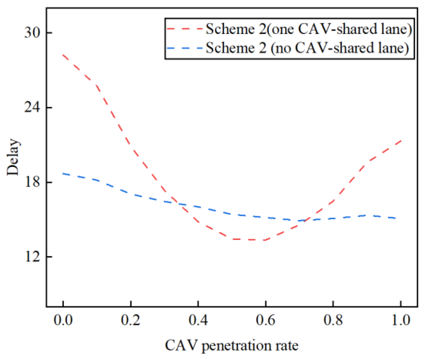
Sensitivity analysis is conducted to verify that the number of CAV-shared lanes is closely dependent on the CAV penetration rate.

And the contribution of our study to sustainability is mainly reflected in the following aspects:

(1)

Promote sustainable development of transportation

Under established road conditions, dynamically configuring CAV-shared lanes can further enhance the traffic capacity of intersections, carry more traffic demands, help save land resources and investments, alleviate traffic congestion, and support the sustainable development of road traffic.

(2)

Promote sustainable development of the environment

Dynamic configuration of CAV-shared lanes can effectively improve vehicle delays on urban roads, achieve the goal of increasing travel speed, help reduce tailpipe emissions, and promote sustainable environmental development.

(3)

Promote sustainable development of energy

Similarly, dynamically configuring CAV-shared lanes not only reduces average vehicle delay and increases travel speed, but also ensures smoother traffic flow, helping to reduce energy consumption and promote sustainable energy development.

The remainder of this paper is organized as follows. Section 2 addresses the gap in the usage of CAV-dedicated lanes and marks different types of approach lanes. Section 3 introduces the method to dynamically allocate and efficiently use the CAV-shared lanes. The numerical experiments are conducted in Section 4, and the results are analyzed in Section 5. Finally, some conclusions and future research are discussed in Section 6.

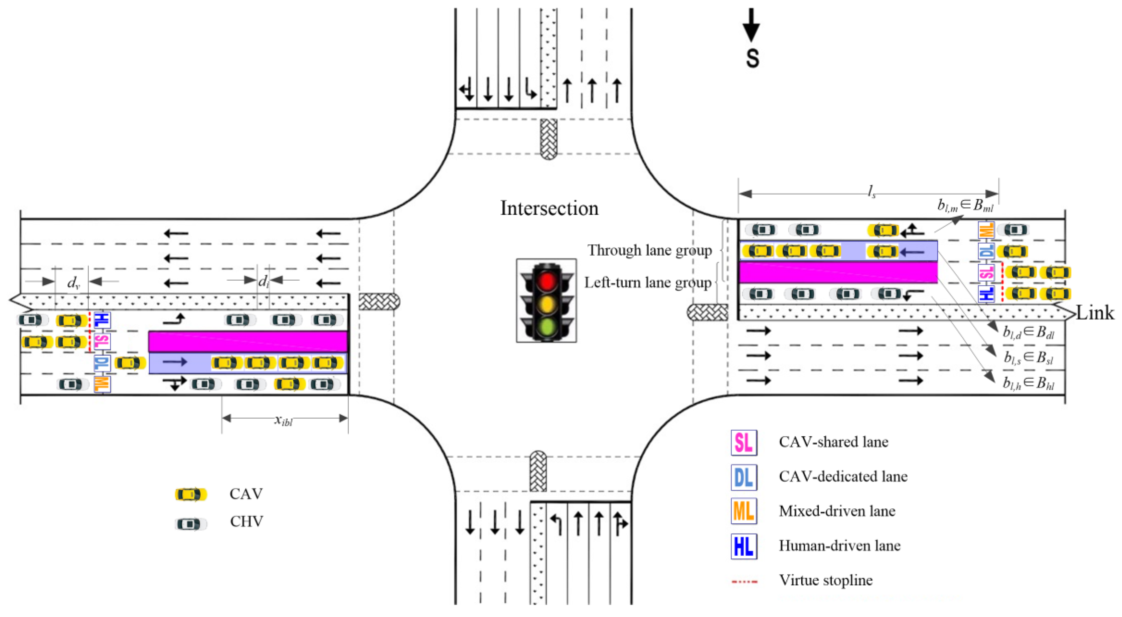
2. Problem Description and Notations

The research conducted by Bahrami and Roorda [17] showed that the saturation flow rate of mixed-driven lanes is affected by the CAV penetration rate, but does not increase linearly, unlike the CAV penetration rate. When the CAV penetration rate is higher than a specific threshold, driving CAVs and CHVs separately will help improve the saturation flow rate of the lane group (and then the phase) and the operation performance of the intersection.

At present, there are two situations for the configuration and use of CAV-dedicated lanes. One is that CAV-dedicated lanes are shared by the left-turn CAVs and through CAVs in an independent phase, such as the blue phase in the literature [15]; the other is that left-turn CAVs and through CAVs use separated CAV-dedicated lanes in their respective phases, such as the dynamic CAV-dedicated lane allocation method proposed by Jiang and Shang [14]. The separated CAV-dedicated lanes are suitable for large-scale mixed traffic flow and multilane intersections, but the shared CAV-dedicated lanes are just the opposite.

Although Jiang and Shang [14] solved the problem associated with the dynamic allocation of CAV-dedicated lanes with the CAV penetration rate and traffic demand to avoid transitions or inefficient use of these lanes, the corresponding time utilization rate was the same as that of other lanes in the lane group. They did not make full use of the characteristics of CAV trajectory controllability, and tapped the traffic potential of CAV-dedicated lanes. Ma et al. [18] both considered the CAV-dedicated lanes and CAV trajectory planning while the left-turn and through CAVs shared the CAV-dedicated lanes, but the allocation of CAV-shared lanes was static and difficult to adapt to the change in the CAV penetration rate. In view of this, this study investigates the dynamic allocation method of CAV-shared lanes to improve the capacity of multilane intersections in mixed CHV and CAV traffic.

In this study, the CAV-shared lane is a kind of CAV-dedicated lane that is shared in turn by the left-turn CAVs and through CAVs. In a cycle, the lane has right of way at least twice. We assume that the CAV and CHV will follow the lane function instructions to change lanes and enter the target lane after entering the link. The CAV trajectory within 300 m of the intersection can be optimized. In this study, L is the set of all lane groups at the intersection and L_i is the set of all lane groups at approach i. B_sl, B_dl, B_hl and B_ml represent the sets of CAV-shared lanes, CAV-dedicated lanes, human-driven lanes, and mixed-driven lanes in the lane group l ∈ L, respectively. Figure 1 shows an example of a supervised intersection.

In Figure 1, when it is necessary to set up CAV-shared lanes at an approach, the lanes are generally located between the left-turn lanes and through lanes. If there is only one CAV-shared lane, the virtual stop-line is set behind the CAV-shared lane and its neighbouring left-turn lane (seen Figure 2). When the number of CAV-shared lanes exceeds one, the virtual stop-line is only arranged behind the CAV-shared lanes (see Figure 3).

In Figure 2, during the red time, the CAVs and CHVs on the lanes with a virtual stop-line queue up at the virtual stop-line. When the left-turn CHVs are not blocked by the left-turn CAVs, they are not constrained by the virtual stop-line and can directly reach the intersection stop-line. For lanes without a virtual stop-line, including CAV-dedicated lanes, human-driven lanes, and mixed-driven lanes, the CAVs and CHVs queue up at the intersection stop-line. In the case shown in Figure 3, all left-turn CAVs and through CAVs queue up in their respective lanes behind the virtual stop-line, while CAVs and CHVs drive separately in the approach lanes of the intersection.

The phase scheme of the intersection is determined by NEMA. Taking one of the phase schemes as an example, i.e., left-turn phase first and then through phase in the east–west direction (seen Figure 4), the release process of traffic flow for each phase is introduced as follows. Like the tandem intersection, the release process is completed in three steps. For the left-turn phase in Figure 2, first, the CAVs and CHVs on the left-turn lane behind the virtual stop-line are guided to enter the CAV-shared lane and left-turn human-driven lane before the phase is activated. Second, the left-turn CAVs and CHVs are released simultaneously when the left-turn light turns on. Last, the left-turn CAVs in the CAV-shared lane need to be cleared and the subsequent left-turn CAVs queue up at the virtual stop-line before the left-turn phase ends. The release process of traffic flow in the through phase is similar to that in the left-turn phase.

3. Method Construction

3.1. Objective Function

In this study, the objective function is shown in Equation (1). In Equation (1), the sum of the flow rate ratios of all lane groups is minimized by reasonably allocating CAV-shared lanes, so that the same traffic demand can be released with the shortest signal cycle.

$$f=\min {\displaystyle \sum _i{\displaystyle \sum _{l\in L_i}\left\{\begin{array}{c}\begin{array}{l}\max \left\{\frac{(1-{\gamma }_l)V_l{p}_{l,cav}}{S_{l,1}(b_{l,d}+b_{l,s})},\frac{V_l(1-p_{l,cav})+{\gamma }_l{V}_l{p}_{l,cav}}{S_{l,2}{b}_{l,h}+S_{l,3}{b}_{l,m}}\right\},\\ \hspace{1em}\hspace{1em}\hspace{1em}\hspace{1em}\hspace{1em}\hspace{1em}\hspace{1em}\hspace{1em}\hspace{1em}\hspace{1em}\hspace{1em}\hspace{1em}{b}_{l,d}+b_{l,s}>0\end{array}\\ \frac{V_l}{S_{l,2}{b}_{l,h}+S_{l,3}{b}_{l,m}},\hspace{0.33em}\hspace{1em}\hspace{1em}\hspace{1em}\hspace{1em}\hspace{1em}\hspace{1em}\hspace{0.33em}\hspace{0.33em}\hspace{0.33em}{b}_{l,d}+b_{l,s}=0\end{array}\right.}}$$

(1)

where b_l,s is the number of CAV-shared lanes in lane group l ∈ L, b_l,d is the number of CAV-dedicated lanes in lane group l ∈ L, b_l,h is the number of human-driven lanes in lane group l ∈ L, and b_l,m is the number of mixed-driven lanes in lane group l ∈ L. The saturation flow rates of the CAV-dedicated lane or CAV-shared lane, human-driven lane and mixed-driven lane in lane group l ∈ L are given by S_l,1, S_l,2 and S_l,3, respectively. V_l is the traffic volume of lane group l ∈ L, p_l,cav is the CAV penetration rate of lane group l ∈ L and γ_l represents the proportion of right-turn vehicles.

In Equation (1), the flow rate ratio of a lane group is determined by the maximum flow rate ratio of each lane. The first item indicates that when there are CAV-dedicated or CAV-shared lanes in the lane group, CAVs and CHVs travel on the corresponding lanes respectively. At this time, it is necessary to calculate the flow rate ratio of different types of lanes (CAV-dedicated lane/CAV-shared lane, human-driven lane and mixed-driven lane) separately and take the maximum value. The second item indicates that all lanes are mixed-driven lanes, and the flow rate ratio only needs to be calculated based on the type of mixed-driven lane.

When the number of approach lanes is not less than three, the allocation of CAV-dedicated lanes must meet the conditions below:

If b_l,d > 0, then

$$\begin{array}{l}\max [{\displaystyle \frac{(1-{\gamma }_l)V_l{p}_{l,cav}}{S_{l,1}(b_{l,d}^{\prime }+b_{l,s})}},{\displaystyle \frac{V_l(1-p_{l,cav})+{\gamma }_l{V}_l{p}_{l,cav}}{S_{l,2}{b}_{l,h}^{\prime }+S_{l,3}{b}_{l,m}^{\prime }}}]\le \\ \max [{\displaystyle \frac{(1-{\gamma }_l)V_l{p}_{l,cav}}{S_{l,1}{b}_{l,d}}},{\displaystyle \frac{V_l(1-p_{l,cav})+{\gamma }_l{V}_l{p}_{l,cav}}{S_{l,2}{b}_{l,h}+S_{l,3}{b}_{l,m}}}]\hspace{1em}\forall l\in L_i\end{array}$$

(2)

Otherwise,

$$\begin{array}{l}\max [{\displaystyle \frac{(1-{\gamma }_l)V_l{p}_{l,cav}}{S_{l,1}{b}_{l,s}}},{\displaystyle \frac{V_l(1-p_{l,cav})+{\gamma }_l{V}_l{p}_{l,cav}}{S_{l,2}{b}_{l,h}^{\prime }+S_{l,3}{b}_{l,m}^{\prime }}}]\le \\ \max [{\displaystyle \frac{V_l}{S_{l,2}{b}_{l,h}+S_{l,3}{b}_{l,m}}}]\hspace{1em}\forall l\in L_i\end{array}$$

(3)

$$b_{l,e}\ge b_{l,s}+b_{l,d}+b_{l,h}+b_{l,m}$$

(4)

$$b_i=b_{l,s}+{\displaystyle \sum _{l\in L_i}(b_{l,d}+b_{l,h}+b_{l,m})}$$

(5)

where b_i is the number of lanes at approach I and b_l,e is the number of exit lanes corresponding to lane group l.

3.2. Dynamic Allocation Method for CAV-Shared Lanes

This study uses the saturation level (s_l) and redistribution index (RI_i) to establish the dynamic allocation method of CAV-shared lanes for each approach at the intersection.

3.2.1. One or More CAV-Shared Lanes at Approach i

s_l is expressed by the saturation level of CAV-shared lanes, as follows:

$$s_l=\underset{b}{\min }\{V_l{p}_{l,cav}{h}_{bl}/[g_{l,k}(b_{l,s}+b_{l,d})]\}\hspace{1em}\forall l\in L_i$$

(6)

The method for establishing the redistribution index is as follows:

$$R{I}_i=\max (R{I}_{bl,1},R{I}_{bl,2})\hspace{1em}\forall l\in L_i$$

(7)

$$R{I}_{bl,1}=\left\{\begin{array}{c}R{I}_{bl,1}+1,\hspace{0.17em}if\hspace{0.17em}{s}_l\in [0,{\epsilon }_1]\\ 0\hspace{1em}\hspace{0.33em}\hspace{0.33em}\hspace{0.33em}\hspace{0.33em}\hspace{0.33em}\hspace{0.33em}\hspace{0.33em}\hspace{0.33em}\hspace{0.33em}\hspace{0.33em}\hspace{0.33em},\hspace{0.17em}otherwise\end{array}\right.\hspace{0.33em}\hspace{0.33em}\forall l\in L_i$$

(8)

$$R{I}_{bl,2}=\left\{\begin{array}{c}R{I}_{bl,2}+1\hspace{0.17em},if\hspace{0.17em}{s}_l\in [{\epsilon }_2,1]\\ 0\hspace{1em}\hspace{0.33em}\hspace{0.33em}\hspace{0.33em}\hspace{0.33em}\hspace{0.33em}\hspace{0.33em}\hspace{0.33em}\hspace{0.33em}\hspace{0.33em}\hspace{0.33em}\hspace{0.33em},\hspace{0.17em}otherwise\end{array}\right.\hspace{0.33em}\hspace{0.33em}\forall l\in L_i$$

(9)

Equations (8) and (9) show that when sl is under low (unsaturated traffic) or high demand (oversaturated traffic) levels, 1 is added to the redistribution index; otherwise, the redistribution index is reset to 0.

3.2.2. No CAV-Shared Lanes at Approach i

If b_l,d > 0, s_l is replaced by the saturation level of CAV-dedicated lanes in lane group l, as follows:

$$s_l=\underset{b}{\min }[V_l{p}_{l,cav}{h}_{bl}/(g_{l,k}{b}_{l,d})]\hspace{1em}\forall l\in L_i$$

(10)

Otherwise,

$$s_l=\underset{b}{\min }\{V_l{h}_{bl}/[g_{l,k}(b_{l,h}+b_{l,m})]\}\hspace{1em}\forall l\in L_i$$

(11)

The redistribution index is built as follows:

$$R{I}_i=\max (R{I}_l)\hspace{1em}\forall l\in L_i$$

(12)

$$R{I}_l=\left\{\begin{array}{c}R{I}_l+1\hspace{0.17em},if\hspace{0.17em}{s}_l\ge {\epsilon }_2\\ 0\hspace{0.33em},\hspace{0.17em}\hspace{1em}otherwise\end{array}\right.\hspace{0.33em}\hspace{0.33em}\forall l\in L_i$$

(13)

When the CAV-shared lane allocation for future signal cycles is restarted, the traffic volume and CAV penetration rate of each lane group should be predicted. In this study, a tensor-based approach [19] is used to predict the short-term traffic flow. In the prediction process, the generation method of historical data can be seen in the literature [14]. The time step of the prediction data is 5 min, with no less than three signal cycles. To avoid repeated predictions within a time step, the time interval for reactivating the lane function allocation should not be less than one time step of the predicted data. Therefore, we use 3 as the threshold of the redistribution index. When RI_i = 3, the number of CAV-shared lanes at approach i is reallocated according to Equation (1) and constraints (2)–(5); after which it is reset to RI_bl,1 = 0, RI_bl,2 = 0, RI_l = 0, and RI_i = 0. According to two studies [20,21], ε₁ = 0.6 and ε₂ = 0.9 are suitable.

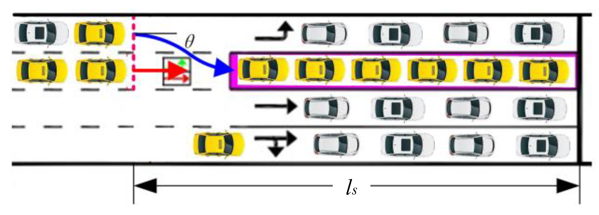
3.3. Traffic Flow Scheduling for CAV-Shared Lanes

For the CAV-shared lanes, the scheduling of left-turn CAVs and through-CAVs with the signal phase is shown in Figure 5. Here, h_bl is the saturated headway of lane b in lane group l, and l_s is the distance from the virtual stop-line to intersection stop-line.

3.3.1. Dynamic Virtual Stop-Line

To avoid left-turn CHVs blocking the virtual stop-line shown in Figure 2, and consider the volatility of traffic flow, the position l_s of the virtual stop-line varies with the traffic volume and CAV penetration rate of the left-turn lane group at approach i, as shown below:

$$l_s=V_l\times (1-p_{l,cav})/(2b_{l,h})\times (d_v+d_s)\hspace{0.33em}+v_{cross}^2/2a_1,\hspace{0.33em}\hspace{0.33em}l\hspace{0.17em}\mathrm{is}\hspace{0.33em}\mathrm{left}\text{-}\mathrm{turn}\hspace{0.33em}\mathrm{lane}\hspace{0.33em}\mathrm{group}$$

(14)

Here, V_l is the prediction traffic volume of left-turn lane group l (pcu/5 min), p_l,cav is the prediction CAV penetration rate of lane group l (%), a₁ is the desired acceleration or deceleration of CAV, v_cross represents the target speed in the approach lane, d_v represents the length of the vehicle, and d_s is the desired safety distance between adjacent CHVs in queuing. In Equation (14), the first item is the maximum queue length of left-turn CHVs per cycle, and the second item is the desired distance travelled when the CAV accelerates to target speed.

In the case shown in Figure 3, l_s depends on the maximum queue length for left-turn CAVs and through CAVs per lane in one signal cycle at approach i, as shown below:

$$l_s=\max [V_l\times p_{l,cav}/2(b_{l,s}+b_{l,d})\times (d_v+d_i)\hspace{0.33em}]\hspace{1em}\forall l\hspace{0.17em}\in L_i$$

(15)

where d_i is the desired safety distance between adjacent CAVs in queuing.

3.3.2. Starting and Close Times of Scheduling at the Virtual Stop-Line

(1)

Starting time

When there is only one CAV-shared lane, to minimize the stops of CAVs as much as possible, it is best for the first CAV behind the virtual stop-line to reach the intersection stop-line just in time for the green light to turn on; the starting time of scheduling for CAVs at the virtual stop-line is as follows:

$$t_{v,k}^o=t_{l,k}-v_{cross}/a_1-(l_s-v_{cross}^2/2a_1)/v_{cross}$$

(16)

where $t_{v,k}^o$ is the scheduling starting time for CAVs at the virtual stop-line of the k^th cycle; t_l,k is the green light starting time of lane group l of the k^th cycle.

If the number of CAV-shared lanes exceeds one, it is necessary to ensure that CAVs can smoothly fill the CAV-shared lanes before the phase is activated, so the starting time of scheduling for CAVs at the virtual stop-line can be determined by follows:

$$t_{v,k}^o=t_{l,k}-[v_{cross}/a_1+(l_s-v_{cross}^2/2a_1)/v_{cross}]\times b_{l,s}$$

(17)

(2)

Close time

To clear the CAV-shared lanes, all CAVs in the CAV-shared lanes must cross the intersection stop-line before the phase green light is turned off. Based on this, the close time of scheduling for CAVs at the virtual stop-line is established as follows:

$$t_{v,k}^c=t_{l,k}+g_{l,k}-(l_s+v_{cross}^2/2a_1)/v_{cross}$$

(18)

where g_l,k is the green time of the kth cycle of lane group l, $t_{v,k}^c$ is the scheduling close time for CAVs at virtual stop-line of the k^th cycle.

In Equation (18), the last item time is used to ensure that the CAVs can still cross the intersection stop-line before the phase green light is turned off, when it is difficult to stop smoothly behind the virtual stop-line.

3.3.3. Platoon Division of CAVs

(1)

For mixed-driven lanes behind the virtual stop-line

When there is only one CAV-shared lane, the left-turn lane behind the virtual stop-line is a mixed-driven lane, and the CHV is uncontrollable, resulting in limited controllability of left-turn CAVs behind the virtual stop-line. Therefore, each CAV near the virtual stop-line is scanned; if $x_{ibl}(t_{v,k}^c)\ge l_s+v_{ibl}^2(t_{v,k}^c)/2a_1$ and $x_{i-1,bl}(t_{v,k}^c)<l_s+v_{i-1,bl}^2(t_{v,k}^c)/2a_1$, CAV i is the first controlled vehicle to be stopped at the virtual stop-line after the end time. Here, v_ibl(t) is the speed of vehicle i on lane b in lane group l at time t and x_ibl(t) is the relative distance of vehicle i at time t from the beginning of lane b in lane group l.

(2)

For CAV-dedicated lanes behind the virtual stop-line

When the green light is on, the shortest time that the CAV i at location x_ibl(t_l,k) requires to cross the intersection stop-line without obstruction from the front CAV can be calculated as follows:

$${\rho }_{ibl}^{\prime }(t_{l,k})=\left\{\begin{array}{l}2\sqrt{x_{ibl}(t_{l,k})/a_{acc}+0.5[v_{cross}^2+v_{ibl}^2(t_{l,k})]/a_{acc}^2}-[v_{cross}+v_{ibl}(t_{l,k})]/a_{acc},\\ \hspace{1em}\hspace{1em}\hspace{1em}\hspace{1em}\hspace{1em}\hspace{1em}\hspace{1em}\hspace{1em}\hspace{1em}\hspace{1em}\hspace{1em}\hspace{1em}\hspace{1em}{x}_{ibl}(t_{l,k})\le [v_{\max }^2-0.5v_{cross}^2-0.5v_{ibl}^2(t_{l,k})]/a_{acc}\\ [v_{\max }-v_{ibl}(t_{l,k})]/a_{acc}+(v_{\max }-v_{cross})/a_{acc}+[x_{ibl}(t_{l,k})-0.5(v_{\max }^2-v_{ibl}^2(t_{l,k}))/a_{acc}\\ -0.5(v_{\max }^2-v_{cross}^2)/a_{acc}]/v_{\max },\hspace{0.33em}\hspace{0.33em}\hspace{0.33em}\hspace{1em}{x}_{ibl}(t_{l,k})>[v_{\max }^2-0.5v_{cross}^2-0.5v_{ibl}^2(t_{l,k})]/a_{acc}\end{array}\right.$$

(19)

$${\rho }_{ibl}(t_{l,k})=\left\{\begin{array}{l}{\rho }_{ibl}^{\prime }(t_{l,k}),\hspace{1em}\hspace{1em}\hspace{1em}\hspace{1em}\hspace{1em}\hspace{0.33em}\hspace{0.33em}\hspace{0.33em}\hspace{0.33em}\hspace{0.33em}\hspace{0.17em}\hspace{1em}\hspace{0.33em}\hspace{0.33em}i=1\\ \max ({\rho }_{i-1,bl}^{\prime }(t_{l,k})+h_{bl},{\rho }_{ibl}^{\prime }(t_{l,k})),\hspace{0.33em}\hspace{0.33em}\hspace{0.17em}i>1\end{array}\right.$$

(20)

where a_acc is the maximum acceleration/deceleration.

In Equation (19), the first part represents the time required for the acceleration process, the second part is the time required for the deceleration process from a uniform speed to the target speed, and the third part is the travel time at a uniform speed. Equation (20) is the adjusted shortest time, which not only considers the obstruction of the preceding CAV, but also allows CAVs to leave the intersection stop-line at a saturated headway.

If ρ_ibl(t_l,k) ≤ g_l,k and ρ_i+1,bl(t_l,k) > g_l,k, the CAV i in transit is the last vehicle released in this phase, and its trajectory needs to be optimized to cross the stop-line. The following CAVs are processed in the next signal cycle.

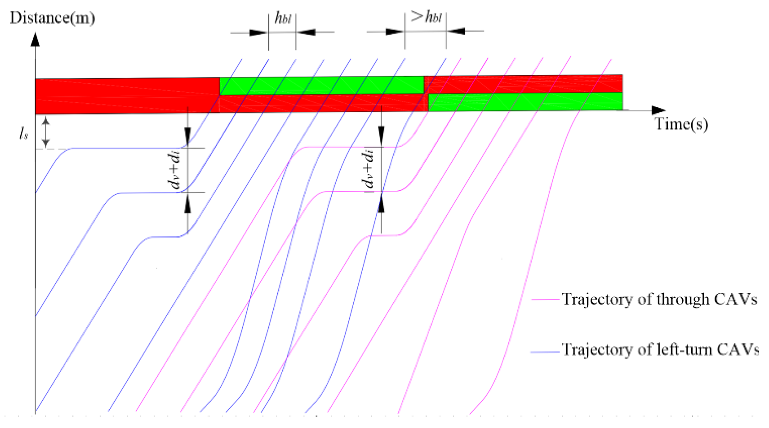
3.4. Trajectory Control Models

3.4.1. Trajectory Constraints

$$v_{ibl}(t+\Delta t)=v_{ibl}(t)+a_{ibl}(t)\Delta t$$

(21)

$$x_{ibl}(t+\Delta t)=x_{ibl}(t)-v_{ibl}(t)\Delta t-0.5a_{ibl}(t)\Delta t^2$$

(22)

$$v_{\min }\le v_{ibl}(t)\le v_{\max }$$

(23)

$$-a_{acc}\le a_{ibl}(t)\le a_{acc}$$

(24)

where a_ibl(t) is the acceleration of vehicle i on lane b in lane group l at time t and the maximum speed and minimum speeds are given by v_max and v_min, respectively.

Equations (21) and (22) are the basic equations of motion used to update the vehicular speed and position, and Equations (23) and (24) are the general constraints of vehicular speed and acceleration.

3.4.2. Trajectory Optimization Models

For human-driven lanes or mixed-driven lanes, the trajectory update of the CHV following the front vehicle (CAV or CHV) adopts the car-following model improved by Panwai and Dia [22], as follows:

$$a_{ibl}(t)={\alpha }_1(v_{i-1,bl}(t)-v_{ibl}(t))+{\alpha }_2((x_{i-1,bl}(t)-x_{ibl}(t)-d_v)-d_s-{\tau }_h{v}_{ibl}(t))\hspace{0.33em}$$

(25)

where τ_h is the reaction time of CHVs.

The intelligent driver model (IDM) is selected as the car-following model of CAV, as follows:

$$a_{ibl}(t)=a_{acc}\times [1-{({\displaystyle \frac{v_{ibl}(t)}{v_{\cos s}}})}^4-{({\displaystyle \frac{s^{*}(v_{ibl}(t),\Delta v_{ibl}(t))}{\Delta x_{ibl}(t)-d_v}})}^2]$$

(26)

$$s^{*}(v_{ibl}(t),\Delta v_{ibl}(t))=d_i+h_{bl}{v}_{ibl}(t)-{\displaystyle \frac{v_{ibl}(t)\Delta v_{ibl}(t)}{2\sqrt{a_{acc}{a}_1}}}$$

(27)

For CAV-shared lanes or CAV-dedicated lanes, the trajectory optimization of the following CAV is shown in Figure 6.

In Figure 6, to ensure smooth trajectory and riding comfort while maximizing the use of CAV-shared lanes, a minimum constant acceleration or deceleration needs to be found for each CAV, so that the i^th CAV at time $t_{v,k}^o$ and location x_ibl($t_{v,k}^o$) can depart from the intersection stop-line at the expected time $\max [t_{l,k}-t_{v,k}^o+(i-1)\times h_{bl},{\rho }_{ibl}(t_{v,k}^o)]$ with saturation headway h_bl and target speed v_cross. The optimization process of the i^th CAV following front vehicle can be divided into five stages (see Figure 7 and Equation (29)): constant speed stage, acceleration (deceleration) stage, another constant speed stage, deceleration (acceleration) stage, and following stage at the target speed v_cross.

The trajectory optimization for each CAV can be expressed as follows:

$$\min a_{ibl}\hspace{0.33em}$$

(28)

where s.t.: (23), (24), and

$$v_{ibl}(t+\Delta t)=\left\{\begin{array}{c}{v}_{ibl}(t_{v,k}^o),\hspace{0.17em}\hspace{1em}\hspace{1em}\hspace{0.33em}\hspace{0.33em}t\in [t_{v,k}^o,t_{v,k}^o+t_5)\\ v_{ibl}(t)\pm a_{ibl}\Delta t,\hspace{0.33em}\hspace{0.17em}t\in [t_{v,k}^o+t_5,t_{v,k}^o+t_5+t_4)\\ v_{ibl}(t),\hspace{0.17em}\hspace{1em}\hspace{1em}\hspace{1em}t\in [t_{v,k}^o+t_5+t_4,t_{v,k}^o+t_5+t_4+t_3)\\ v_{ibl}(t)\mp a_{ibl}\Delta t,\hspace{0.33em}t\in [t_{v,k}^o+t_5+t_4+t_3,t_{v,k}^o+t_5+t_4+t_3+t_2)\\ v_{cross},\hspace{0.33em}\hspace{0.33em}\hspace{0.33em}t\in [t_{v,k}^o+t_5+t_4+t_3+t_2,t_{v,k}^o+t_5+t_4+t_3+t_2+t_1)\end{array}\right.\hspace{0.33em}$$

(29)

$$t_5+t_4+t_3+t_2+t_1=\max [t_{l,k}-t_{v,k}^o+(i-1)\times h_{bl},{\rho }_{ibl}(t_{v,k}^o)]$$

(30)

3.5. Solution Process of Optimization Model

In this study, two objective functions need to be solved. For the solution of the CAV-shared lane configuration in Equation (1), subject to the constraints (2)–(5), the branch and bound method can be used to solve it quickly and the calculation scale is small.

The trajectory optimization in Equation (28) is a linear solving problem, subject to the constraints (23), (24), (29) and (30), which can be used to easily find a_ibl, t₁, t₂, t₃, t₄, and t₅. The flow chart outlining the solution is shown in Figure 8.

4. Numerical Experiments

4.1. Basic Conditions

The values of relevant parameters in this study are listed in

Table 1. Value of the parameters used in this study.

Parameter Names	Value
Maximum speed (m/s)	13
Minimum speed (m/s)	4
Speed limit of the intersection (m/s)	11
Maximum acceleration (m/s2)	4
Desired acceleration (m/s2)	2.5
Trajectory updating interval (s)	0.5
Minimum green time for left-turning movements (s)	12
Maximum green time for left-turning movements (s)	45
Minimum green time for through and right-turning movements (s)	12
Maximum green time for through and right-turning movements (s)	60
Average length of vehicles (m)	4
Safe space between adjacent CAVs in queuing (m)	0.5
Safety distance between consecutive vehicles (m)	3.6
The reaction time for CAVs (s)	0.1
The reaction time for CHVs (s)	1.0
Saturation headway between CAV-CAV and CAV-CHV (s)	1
Saturation headway between CHV-CHV and CHV-CAV (s)	2
Saturation flow rate of the CAV-dedicated lane and CAV-shared lane for through movements (pcu/h)	3600
Saturation flow rate of the human-driven lane for through movements (pcu/h)	1800
Saturation flow rate of the CAV-dedicated lane and CAV-shared lane for left-turn movements(pcu/h)	3200
Saturation flow rate of the human-driven lane for left-turn movements (pcu/h)	1600
Study period (s)	3600

by referring to various studies [1,14,16,23]. An algorithm is developed to update the vehicular trajectory and exchange information between CAV/CHV and the signal controller based on the COM component in VISSIM (5.3, PTV AG, Karlsruhe, Germany). The traffic flow detector is set on the lane in VISSIM to collect the time and speed of each vehicle entering the link every 0.5 s, and the vehicular acceleration, speed, and position are updated every 0.5 s.

Taking the intersection in Figure 1 as an example, the lengths of east, west, south, and north links are all set to 400 m. The hourly traffic volumes of all approaches are listed in

Table 2. Traffic volume per hour.

Approach	Traffic Volume/(pcu·h−1)
	Left-Turn		Through and Right-Turn
	CHV	CAV	CHV	CAV
East	128	137	506	518
West	125	142	494	537
South	133	154	487	509
North	161	175	533	558

. Among them, the proportion of right-turns for CAVs is 0.03. The traffic conditions are the same as that of the literature [14].

4.2. Simulation Scheme

Three simulation schemes are designed for comparative analysis. Scheme 1 is the dynamic CAV-dedicated lane allocation method proposed by Jiang and Shang [14], Scheme 2 is the optimization strategy proposed in this study, and Scheme 3 is the shared-phase dedicated-lane method proposed by Ma et al. [18].

5. Result and Discussion

5.1. Result Analysis

Table 3. Stop rate.

Plan	Approach	Phase 1	Phase 2	Approach	Phase 3	Phase 4	All
Scheme 1	East	0.69	0.64	South	0.70	0.71	0.69
	West	0.70	0.65	North	0.69	0.70
Scheme 2	East	0.74	0.75	South	0.74	0.75	0.74 (↑7.47%)
	West	0.73	0.74	North	0.75	0.76

Note: ↑ denotes an increase, compared with Scheme 1.

,

Table 4. Average delay.

Plan	Approach	Phase 1	Phase 2	Approach	Phase 3	Phase 4	All
Scheme 1	East	11.43	10.79	South	11.37	11.94	11.36
	West	11.37	10.89	North	11.45	11.79
Scheme 2	East	11.05	10.37	South	10.29	10.71	10.65 (↓6.25%)
	West	11.02	10.34	North	10.36	10.82

Note: ↓ represents a decrease, compared with Scheme 1.

and

Table 5. Time utilization rate per lane.

Plan	Left-Turn Lane	CAV-Shared Lane	Through Lane	Sharing Lane for Through and Right-Turn Vehicles
Scheme 1	0.24	0.21	0.21	0.23
Scheme 2	0.16 (↓33.33%)	0.43 (↑100.50%)	0.27 (↑28.57%)	0.29 (↑26.09%)

Note: ↓ represents a decrease, and ↑ denotes an increase, compared with Scheme 1.

show the results of traffic simulation. The percentages in brackets in Table 3 and Table 4 are the changes in Scheme 2 compared with Scheme 1. In addition, we compare the differences in the time resource utilization of the approach lane, as shown in Table 5.

In Table 3 and Table 4, the delay of Scheme 2 decreases by 6.25% compared with Scheme 1. The reason is attributed to the fact that the CAV-shared lanes are composite utilization lanes between left-turn CAVs and through-CAVs. Scheme 2 does not change the traffic condition of through vehicles in Scheme 1, but considerably improves the traffic condition of left-turn vehicles; this is equivalent to adding an additional CAV-dedicated left-turn lane. At the same traffic volume, the green time required for left-turn vehicles is only approximately 60% of that in Scheme 1, which not only reduces the green time of the left-turn phase, but also shortens the signal cycle. Therefore, the delay of each phase decreases to varying degrees.

However, the disadvantage of Scheme 2 compared with Scheme 1 is the fact that the stop rate increases by 7.47%; this is attributed to the secondary stops of some CAVs since the CAV-shared lane is used alternately to release the left-turn CAVs and through CAVs. At the same time, left-turn CAVs waiting to enter the CAV-shared lane will cause some subsequent left-turn CHVs to stop in front of the virtual stop-line and then need to stop twice in front of the stop-line to wait for green time. In order to reduce the stop rate, we can plan the trajectories of vehicles that arrive at the virtual stop-line after the time $t_{v,k}^o$ to travel at the minimum speed, so that these vehicles do not stop at the virtual stop line, thereby reducing the stop rate.

From Table 5, it can be inferred that except for human-driven left-turn lanes, the time utilization rates of other lanes in Scheme 2 improve considerably compared with those in Scheme 1, particularly the CAV-shared lane, as shown in Figure 9a. The blue lines of Figure 9a represent the trajectory of left-turn CAVs, and the red lines are those of the through CAVs. The reason is attributed to the fact that the CAV-shared lane shares nearly half of the left-turn vehicles, which reduces the green time required for mixed-driven vehicles in the left-turn lane by 40%; thus, the ratio of left-turn phase green time in the signal cycle decreases abruptly. Therefore, the time utilization rate of human-driven left-turn lane decreases rapidly, whereas that of all lanes in the through phase increases abruptly. The key to the higher temporal utilization of the CAV-shared lane is that irrespective of the left-turn or through-phases, it is used consistently, and its time utilization rate is the sum of that of left-turn and through phases. Figure 9b,c describe the trajectory of CHVs in the human-driven left-turn and human-driven through lanes. There are two types of stops in Figure 9b, one behind the approach stop line and the other behind the virtual stop line. The determination of the stop spatial location depends on whether the vehicle in front of the CHV is a CAV or not when it arrives at an intersection during the red time. Given that there are no CAVs in the human-driven through lane, the CHVs arriving at the intersection during the red time will wait in line directly behind the approach stop line.

Although the CAV-shared lane control strategy proposed in this study increases the stops of the CAVs, the total vehicular delay is decreased and the time utilization rate of most approach lanes improves considerably; this change can effectively improve the capacity of the intersections. Therefore, the optimal control method proposed in this study is feasible and effective. Compared with conventional static control (left-turn and through waiting area) and unconventional dynamic control (such as comprehensive waiting area, continuous flow intersection), this dynamic lane configuration method utilizes the controllable trajectory of CAVs to eliminate the front pre-signals. And the number of CAV-shared lanes and the position of front pre-signals can be dynamically adjusted based on real-time traffic flow and the CAV penetration rate. Not only has it improved the traffic efficiency at intersections and optimized the trajectory of vehicles, but it has also enhanced the overall adaptability of the transportation system.

After the CAV-shared lanes are adopted, during the process of alternately releasing left-turn vehicles and through vehicles, the traditional phase scheme is still used, which will not affect the safety of pedestrians crossing the street. When releasing through vehicles, pedestrians in the same direction can safely cross the street; when left-turn vehicles are released, pedestrians on the approach lanes in the intersecting direction and the exit lanes in the current direction can cross the street. The establishment and cancellation of dynamic CAV-shared lanes can cause certain safety hazards and traffic flow disruptions at intersections due to the interaction between CAVs and CHVs. To avoid such situations, it is necessary to install a portal style dynamic lane function indicator in front of the virtual stop-line lane to provide advance notice of lane function. Although this will increase construction costs under actual road conditions, in the long run, the following benefits will be felt:

(1)

This clearly indicates the correct lane for CAVs and CHVs to travel, which can improve the efficiency of traffic flow, reduce delays, and ultimately enhance capacity at intersections.

(2)

This can effectively reduce the situation of CHVs accidentally entering CAV-shared lanes, lower the potential risk of traffic accidents, especially in mixed traffic environments, and improve the safety of pedestrians and vehicles.

Table 6. Average delay for three demand levels with different CAV penetration rates.

Demand	50% CAVs		80% CAVs
Level	Shared-Phase Dedicated Lane	Proposed Method	Shared-Phase Dedicated Lane	Proposed Method
1	7.47	7.11 (↓4.82%)	7.73	6.82 (↓11.77%)
2	10.69	10.65 (↓0.37%)	11.24	10.19 (↓9.34%)
3	15.33	15.31 (↓0.13%)	16.01	14.41 (↓9.99%)

Note: ↓ represents a decrease, compared with Shared-Phase Dedicated Lane.

shows the delay difference between the shared-phase dedicated lane and the optimization strategy proposed in this study in three traffic demand levels with different CAV penetration rates. In Table 6, values 1, 2, and 3 in the first column represent the input traffic volumes that are 0.5, 1, and 1.5 times those listed in Table 2, respectively.

As the traffic demand increases from low to high levels, the method proposed in this study can reduce the delay by 4.82%, 0.37%, and 0.13%, respectively, compared with the shared-phase dedicated lane for a 50% CAV penetration rate. Since the traffic volume per signal cycle is relatively stable at medium to high levels, the two methods have the same requirement for CAV-shared lanes, i.e., one lane. However, the traffic volume and CAV penetration rate fluctuate greatly under a low level and partial signal cycles without CAV-shared lanes have better traffic performance.

At a CAV penetration rate equal to 80%, the proposed method is more effective than the shared-phase dedicated lane, and the delay decreases by 11.77%, 9.34%, and 9.99%, respectively. The reason is attributed to the fact that the method of shared-phase dedicated lane only configures one CAV-shared lane, while the actual requirement is two lanes. The proposed method can further reduce the total flow rate ratio of the lane group, compress the signal cycle and green time of each phase, and thus reduce delay more significantly.

Table 6 shows that with the continuous increase in traffic demand, the average delay per vehicle is also growing rapidly. The root cause is that the increase in traffic demand requires longer signal cycles to fully release, resulting in an increase in the time vehicles wait for red lights. And Figure 10 also indicates that under the same traffic demand, as the CAV penetration rate changes, if the lane function configuration is not reasonable, it will also lead to an increase in average vehicle delay. For example, when the CAV penetration rate is low, no CAV-shared lane has a better control effect than that of setting up a CAV-shared lane. However, under a high CAV penetration rate, only setting up one CAV-shared lane will actually increase average vehicle delay. The reason is that a CAV-shared lane actually increases the difference in flow rate ratios between different functional lanes in the same lane group, resulting in a rapid increase in signal cycle, requiring more CAV-shared lanes to balance the flow rate ratios of different functional lanes. Therefore, the CAV penetration rate is the key factor to determine whether to set CAV-shared lanes or not.

Figure 11 shows that the approach lane allocation varies with the predicted CAV penetration rate (P_cav) for the east approach during the simulation.

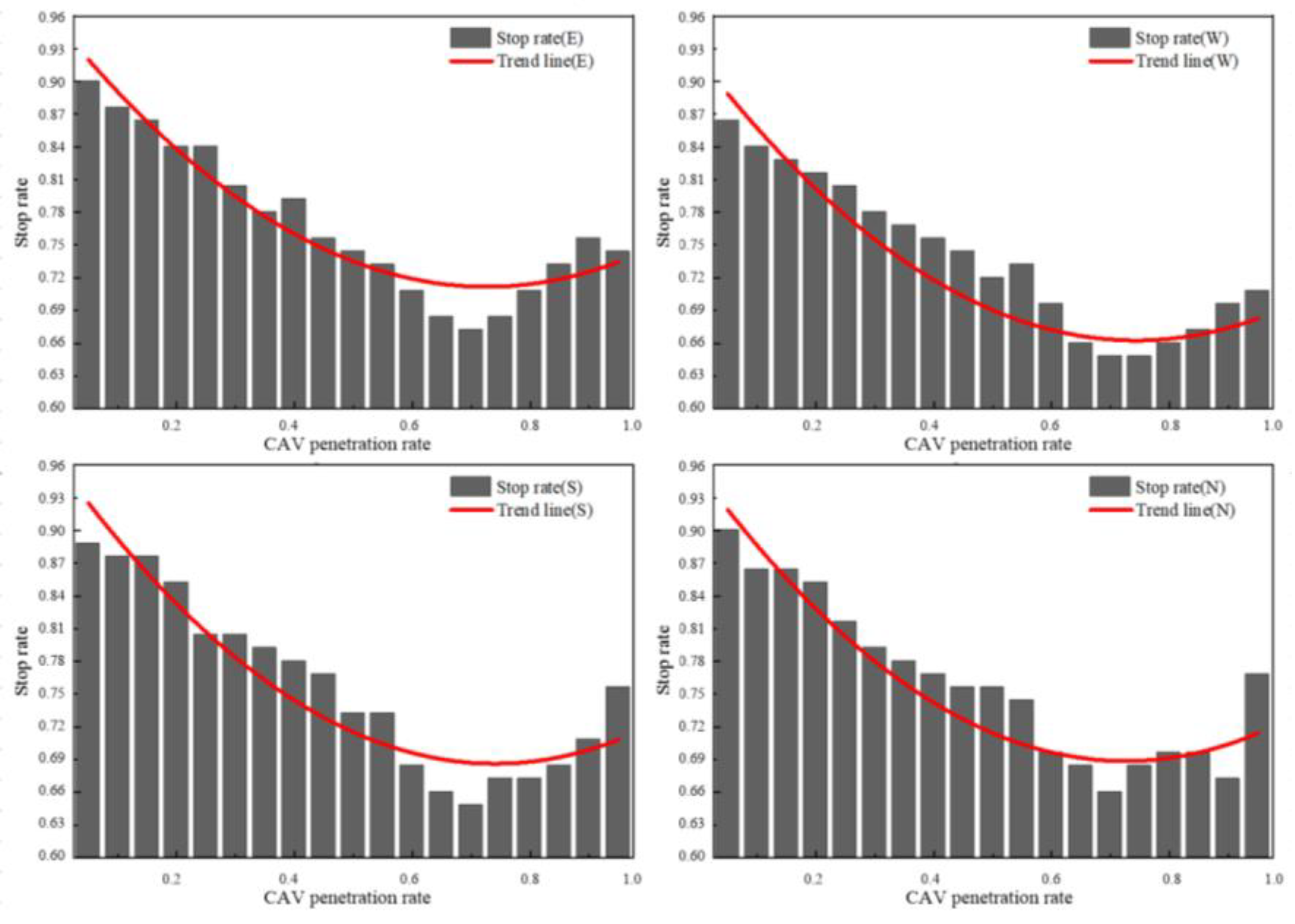
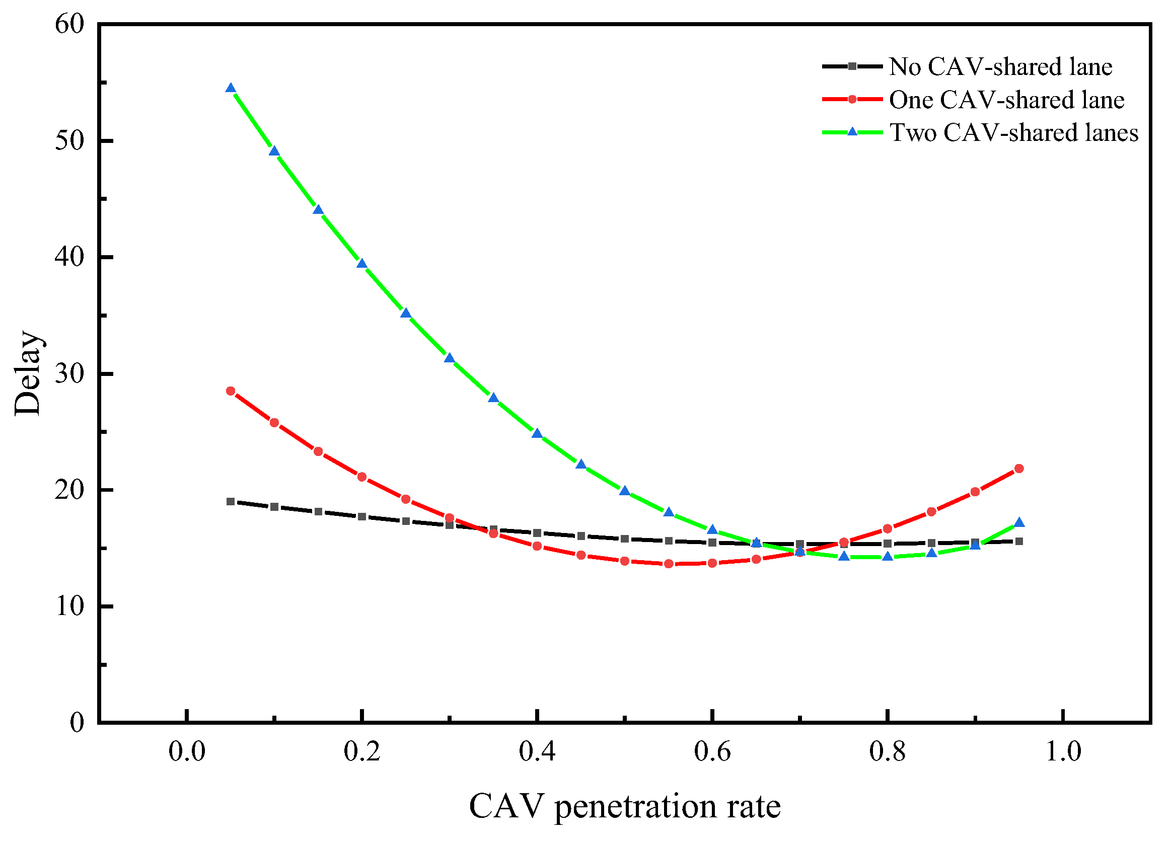
5.2. Sensitivity Analysis

The signal control scheme and the input traffic volume remain unchanged. When there is only one CAV-shared lane, the CAV penetration rate in the traffic flow varies from 0 to 1, with a step-size of 0.05. The simulation results are shown in Figure 12 and Figure 13.

Figure 12 shows that the stop rate decreases to the lowest level when the CAV penetration rate is in the range of 0.6–0.8, and changes in a downward direction at a relatively stable rate as a function of the CAV penetration rate in the range of 0–0.6, but gradually shifts in the upward direction in the CAV penetration rate range of 0.8–1.0. When the CAV penetration rate is lower, more CHVs require longer phase green time at the same traffic volume. Although it is beneficial to optimize the CAV trajectory, the number of CAVs is small, and the increase in the number of stops of CHVs following the prolongation of the phase green time is considerably greater than the reduction in the number of stops of CAVs following the optimization of the CAV trajectory; thus, the stop rate remains high. With the gradual increase in the CAV penetration rate, the positive and negative benefits of stops of CHVs and CAVs are gradually improved, and balance is achieved when the CAV penetration rate is in the range of 0.6–0.8. Given that there is only one CAV-shared lane, when the CAV penetration rate exceeds 0.8, constrained by the upper limit of the phase green time, the excessive CAV traffic demand leads to oversaturated traffic in the CAV-shared lane, but the utilization of human-driven lanes is insufficient. Although it is very beneficial to control the operations of CAVs in queues, the secondary stops of CAVs begin to increase. The higher the CAV penetration rate, the more evident the growth of stops; thus, the stop rate increases gradually.

In Figure 13, the variation tendency of the delay at each approach as a function of the CAV penetration rate is basically consistent with the stop rate, but the lowest delay occurs when the CAV penetration rate is in the range of 0.55–0.7. At this time, the green time utilization rate of the CAV-shared and human-driven lanes in the same phase tends to be the same, and the phase green time and signal cycle required to release the same traffic volume are the shortest; therefore, the delay is the smallest. If the CAV penetration rate is too low or too high, it is not conducive to the balanced utilization of CAV-shared lane and human-driven lanes, which will increase the green time per phase and the signal cycle; thus, the delay increases.

The signal control scheme and input traffic volume remain unchanged, the number of CAV-shared lanes changes from 0 to 2, and the CAV penetration rate varies from 0 to 1 in steps of 0.05. Figure 14 is the simulation results.

The results in Figure 14 show that the delay decreases as the CAV penetration rate decreases when there are no CAV-shared lanes, and gradually tends to be stable. This is attributed to the fact that the increase in the CAV penetration rate will increase the saturation flow rate of the mixed-driven lane. When the traffic volume remains unchanged, the flow rate ratio of the lane group gradually decreases, and the signal cycle is shortened; thus, the delay decreases. After setting the CAV-shared lanes, the delay decreases first and then increases as the CAV penetration rate increases. This is attributed to whether the change in the CAV penetration rate can achieve a balanced use of the human-driven lanes and CAV-shared lanes, and whether the change in saturation flow rate of the lane group caused by the setting of CAV-shared lanes is beneficial to promote the decline in the flow rate ratio of the lane group. In this case, the delay is small; otherwise, it will increase.

In addition, when the number of approach lanes and input traffic volume are constant, whether CAV-shared lanes are required or not, and their required number, are closely related to the CAV penetration rate. From Figure 14, it can be seen that when the CAV penetration rate is less than 0.35, the delay of the blue curve is the lowest, so no CAV-shared lane has the best effect. When the CAV penetration rate is between 0.35 and 0.70, the delay of the red curve is actually lower than the other two, so one CAV-shared lane is the best choice at this time. When the CAV penetration rate exceeds 0.7, although the value of the blue curve is lower than that of the green curve when the CAV penetration rate approaches 1, overall, the delay of the green curve is minimal in most intervals. At this time, it is advisable to set up two or more CAV-shared lanes. It can be inferred that the method proposed in this study is suitable for intersections with a high CAV penetration rate.

The signal control scheme and input traffic volume remain unchanged. Under the conditions of three, four, five and six lanes at the approach, the penetration rate of CAV in the traffic flow is gradually changed from 0 to 1 with a step size of 0.05. The simulation results obtained are as follows.

In Figure 15, it can be seen that the CAV penetration rate for setting a CAV-shared lane is 0.70 when the number of approach lanes is three, while as the number of approach lanes is increased to six, the required penetration rate decreases to 0.30. For schemes with four and five approach lanes, the CAV penetration rate for setting one CAV-shared lane is between 0.33 and 0.58, while a higher CAV penetration rate is required for setting two CAV-shared lanes. When the number of approach lanes is six, the CAV penetration rate for setting three CAV-shared lanes is more than 0.80. Therefore, the higher the CAV penetration rates, the more approach lanes there are and the more CAV-shared lanes need to be set up.

6. Conclusions

(1)

This paper designs a dynamic allocation method of CAV-shared lanes to tap the traffic potential of CAV-dedicated lanes and constructs a traffic flow scheduling and CAV trajectory optimization method for multilane intersections with CAV-shared lanes to improve the traffic performance in mixed CHV and CAV traffic. The simulation results show that the optimization strategy proposed in this study can reduce the average delay at the intersection to varying degrees compared with the control strategy, using (a) the dynamic CAV-dedicated lane allocation method proposed in the literature [14] and (b) the shared-phase dedicated-lane method proposed in the literature [18]. Although the stops of CAVs will be increased, the time utilization rates of most approach lanes are improved considerably, particularly those of CAV-shared lanes. Further analysis shows that the number of CAV-shared lanes is closely dependent on the CAV penetration rate.

(2)

This study only solves the dynamic allocation and signal control of CAV-shared lanes. The impact of additional stops on CHV efficiency, safety, and riding comfort, as well as the impact of CAV trajectory control on energy consumption and exhaust emissions, is not considered.

(3)

In addition, future research can consider the optimization control problem of other transportation modes (such as public transportation, carpooling, and slow traffic) at intersections with dynamic CAV-shared lanes to verify the applicability of this method in complex road environments, thereby further improving the overall efficiency of the transportation system.

References

1. Pourmehrab, M.; Elefteriadou, L.; Ranka, S.; Martin-Gasulla, M. Optimizing Signalized Intersections Performance Under Conventional and Automated Vehicles Traffic. IEEE Trans. Intell. Transp. Syst. 2020, 21, 2864–2873. [Google Scholar] [CrossRef]
2. Shi, H.; Zhou, Y.; Wu, K.; Wang, X.; Lin, Y.; Ran, B. Connected automated vehicle cooperative control with a deep reinforcement learning approach in a mixed traffic environment. Transp. Res. Part C Emerg. Technol. 2021, 133, 103421. [Google Scholar] [CrossRef]
3. Wang, J.; Zheng, Y.; Xu, Q.; Wang, J.; Li, K. Controllability analysis and optimal control of mixed traffic flow with human-driven and autonomous vehicles. IEEE Trans. Intell. Transp. Syst. 2021, 22, 7445–7459. [Google Scholar] [CrossRef]
4. Xiong, B.K.; Jiang, R. Speed advice for connected vehicles at an isolated signalized intersection in a mixed traffic flow considering stochasticity of human driven vehicles. IEEE Trans. Intell. Transp. Syst. 2022, 23, 11261–11272. [Google Scholar] [CrossRef]
5. Mo, Z.; Li, W.; Fu, Y.; Ruan, K.; Di, X. CVLight: Decentralized learning for adaptive traffic signal control with connected vehicles. Transp. Res. Part C Emerg. Technol. 2022, 141, 103728. [Google Scholar] [CrossRef]
6. Wang, Q.; Gong, Y.; Yang, X. Connected automated vehicle trajectory optimization along signalized arterial: A decentralized approach under mixed traffic environment. Transp. Res. Part C Emerg. Technol. 2022, 145, 103918. [Google Scholar] [CrossRef]
7. Tajalli, M.; Hajbabaie, A. Distributed Optimization and Coordination Algorithms for Dynamic Speed Optimization of Connected and Autonomous Vehicles in Urban Street Networks. Transp. Res. Part C Emerg. Technol. 2018, 95, 497–515. [Google Scholar] [CrossRef]
8. Tajalli, M.; Hajbabaie, A. Dynamic Speed Harmonization in Connected Urban Street Networks. Comput. Civ. Infrastruct. Eng. 2018, 33, 510–523. [Google Scholar] [CrossRef]
9. Asadi, B.; Vahidi, A. Predictive Cruise Control: Utilizing Upcoming Traffic Signal Information for Improving Fuel Economy and Reducing Trip Time. IEEE Trans. Control Syst. Technol. 2010, 19, 707–714. [Google Scholar] [CrossRef]
10. Jung, H.; Choi, S.; Park, B.B.; Lee, H.; Son, S.H. Bi-level Optimization for Eco-traffic Signal System. In Proceedings of the IEEE 2016 International Conference on Connected Vehicles and Expo (ICCVE), Seattle, WA, USA, 12–16 September 2016; pp. 29–35. [Google Scholar] [CrossRef]
11. Zhang, Y.; Cassandras, C.G. An impact study of integrating connected automated vehicles with conventional traffic. Annu. Rev. Control. 2019, 48, 347–356. [Google Scholar] [CrossRef]
12. Li, Z.; Elefteriadou, L.; Ranka, S. Signal Control Optimization for Automated Vehicles at Isolated Signalized Intersections. Transp. Res. Part C Emerg. Technol. 2014, 49, 1–18. [Google Scholar] [CrossRef]
13. Guo, Y.; Ma, J.; Xiong, C.; Li, X.; Zhou, F.; Hao, W. Joint Optimization of Vehicle Trajectories and Intersection Controllers with Connected Automated Vehicles: Combined Dynamic Programming and Shooting Heuristic Approach. Transp. Res. Part C Emerg. Technol. 2019, 98, 54–72. [Google Scholar] [CrossRef]
14. Jiang, X.; Shang, Q. A Dynamic CAV-dedicated lane allocation method with the joint optimization of signal timing parameters and smooth trajectory in a mixed traffic environment. IEEE Trans. Intell. Transp. Syst. 2023, 24, 6436–6449. [Google Scholar] [CrossRef]
15. Rey, D.; Levin, M.W. Blue phase: Optimal Network Traffic Control for Legacy and Autonomous Vehicles. Transp. Res. Part B Methodol. 2019, 130, 105–129. [Google Scholar] [CrossRef]
16. Niroumand, R.; Tajalli, M.; Hajibabai, L.; Hajbabaie, A. Joint Optimization of Vehicle-group Trajectory and Signal Timing: Introducing the White Phase for Mixed-autonomy Traffic Stream. Transp. Res. Part C Emerg. Technol. 2020, 116, 102659. [Google Scholar] [CrossRef]
17. Bahrami, S.; Roorda, M.J. Optimal Traffic Management Policies for Mixed Human and Automated Traffic Flows. Transp. Res. Part A Policy Pract. 2020, 135, 130–143. [Google Scholar] [CrossRef]
18. Ma, W.; Li, J.; Yu, C. Shared-phase-dedicated-lane based intersection control with mixed traffic of human-driven vehicles and connected and automated vehicles. Transp. Res. Part C Emerg. Technol. 2022, 135, 103509. [Google Scholar] [CrossRef]
19. Tan, H.; Wu, Y.; Shen, B.; Jin, P.J.; Ran, B. Short-term traffic prediction based on dynamic tensor completion. IEEE Trans. Intell. Transp. Syst. 2016, 17, 1–11. [Google Scholar] [CrossRef]
20. Bretherton, D.; Bodger, M.; Cowling, J. SCOOT-managing congestion communications and control. Traffic Eng. Control 2006, 47, 88–92. [Google Scholar]
21. Dion, F.; Rekha, H.; Kang, Y.S. Comparison of delay estimates at under-saturated and over-saturated pre-timed signalized intersections. Transp. Res. Part B Methodol. 2004, 38, 99–122. [Google Scholar] [CrossRef]
22. Panwai, S.; Dia, H. Comparative Evaluation of Microscopic Car-Following Behavior. IEEE Trans. Intell. Transp. Syst. 2005, 6, 314–325. [Google Scholar] [CrossRef]
23. Yao, H.; Li, X. Decentralized Control of Connected Automated Vehicle Trajectories in Mixed Traffic at an Isolated Signalized Intersection. Transp. Res. Part C Emerg. Technol. 2020, 121, 102846. [Google Scholar] [CrossRef]
Figure 1. Example demonstrating the supervision of an intersection.
Sustainability 16 09706 g001
Figure 2. Single CAV-shared lane utilized by left-turn CAVs and through CAVs.
Sustainability 16 09706 g002
Figure 3. Multiple CAV-shared lanes utilized by left-turn CAVs and through CAVs. (a) Left-turn CAVs; (b) through CAVs.
Sustainability 16 09706 g003
Figure 4. Release diagram of traffic flow. (a) Left-turn phase; (b) through phase.
Sustainability 16 09706 g004
Figure 5. Traffic flow scheduling for the CAV-shared lanes.
Sustainability 16 09706 g005
Figure 6. Trajectory optimization of the following CAV.
Sustainability 16 09706 g006
Figure 7. Speed optimization of the following CAV.
Sustainability 16 09706 g007
Figure 8. Flow chart outlining the solution [14].
Sustainability 16 09706 g008
Figure 9. Trajectory optimization results of partial cycles. (a) CAV-shared lane, (b) human-driven left-turn lane, and (c) human-driven through lane.
Sustainability 16 09706 g009
Figure 10. Delay varies with CAV penetration rate in different schemes.
Sustainability 16 09706 g010
Figure 11. Lane allocation results with predicted CAV penetration rate.
Sustainability 16 09706 g011
Figure 12. Stop rates at each approach with CAV penetration rate.
Sustainability 16 09706 g012
Figure 13. Delay patterns at each approach studied herein as a function of the CAV penetration rate.
Sustainability 16 09706 g013
Figure 14. Delay variations as functions of the CAV penetration rate at different numbers of CAV-shared lanes.
Sustainability 16 09706 g014
Figure 15. The variation in traffic flow rate ratio with CAV penetration rate under different numbers of approach lanes and CAV-shared lanes.
Sustainability 16 09706 g015