Research on Fault Diagnosis of Agricultural IoT Sensors Based on Improved Dung Beetle Optimization–Support Vector Machine

Abstract

The accuracy of data perception in Internet of Things (IoT) systems is fundamental to achieving scientific decision-making and intelligent control. Given the frequent occurrence of sensor failures in complex environments, a rapid and accurate fault diagnosis and handling mechanism is crucial for ensuring the stable operation of the system. Addressing the challenges of insufficient feature extraction and sparse sample data that lead to low fault diagnosis accuracy, this study explores the construction of a fault diagnosis model tailored for agricultural sensors, with the aim of accurately identifying and analyzing various sensor fault modes, including but not limited to bias, drift, accuracy degradation, and complete failure. This study proposes an improved dung beetle optimization–support vector machine (IDBO-SVM) diagnostic model, leveraging the optimization capabilities of the former to finely tune the parameters of the Support Vector Machine (SVM) to enhance fault recognition under conditions of limited sample data. Case analyses were conducted using temperature and humidity sensors in air and soil, with comprehensive performance comparisons made against mainstream algorithms such as the Backpropagation (BP) neural network, Sparrow Search Algorithm–Support Vector Machine (SSA-SVM), and Elman neural network. The results demonstrate that the proposed model achieved an average diagnostic accuracy of 94.91%, significantly outperforming other comparative models. This finding fully validates the model’s potential in enhancing the stability and reliability of control systems. The research results not only provide new ideas and methods for fault diagnosis in IoT systems but also lay a foundation for achieving more precise, efficient intelligent control and scientific decision-making.

1. Introduction

Sensors are used in intelligent decision-making and control systems to obtain various pieces of critical physical information [1]. By analyzing the collected data, these systems, in conjunction with intelligent equipment, achieve precise regulation [2]. However, in practical application scenarios, sensors often face challenges due to harsh environments, unstable power supply, and natural wear and aging, among other factors [3,4], leading to frequent failures. The occurrence of sensor faults can significantly interfere with subsequent decision-making and control outcomes, potentially causing system errors [5,6]. Fault diagnosis is an effective means to address this issue [7], with the core objective being the accurate identification of abnormal or faulty information within sensors. Effective measures are then used to restore the normal function of the damaged sensor or safely isolate it from the system, ensuring that the sensor network can continuously and reliably deliver accurate data to users. These accurate data are crucial for data monitoring and early warning, intelligent decision-making, and intelligent control, significantly enhancing system stability and reliability [8].

To achieve sensor fault diagnosis, researchers have explored three main approaches: model-based, knowledge-based, and data-driven methods [9]. Model-based approaches identify and isolate faults through accurate mathematical representations, reflecting the core fault characteristics of physical systems. However, the accuracy of this method relies on precise system parameters and models, making its application in agriculture challenging, primarily due to the nonlinearity and complexity of real-world objects [10]. Even with theoretically well-established models, the discrepancies between sensor performance in agricultural environments and model assumptions can result in significant errors, affecting the accuracy and reliability of diagnosis [11]. Knowledge-based methods rely on expert systems for fault localization and diagnosis and are commonly used in the automotive and power system fields [12]. In agriculture, uncontrollable variables such as climate changes and soil property variations make it difficult to accurately handle sensor data using simple rules or expert knowledge. Additionally, environmental changes may cause temporary abnormal sensor data, which can easily be confused with actual faults. Handling such data requires a large number of complex rules, making the system difficult to maintain in agricultural applications [13].

The data-driven approach does not rely on precise mathematical models or expert systems; instead, it uses large amounts of sensor data to extract patterns and features through machine learning or statistical algorithms, enabling automatic fault diagnosis. These methods are particularly suitable for nonlinear and complex systems [14]. In agricultural contexts, the vast amount of real-time data generated by sensors provides a solid foundation for data-driven methods, effectively addressing the complexity and dynamics of sensor anomalies. However, traditional machine learning methods like decision trees and their ensemble techniques are prone to overfitting when handling high-dimensional data, especially in dynamic and noisy environments like those of agricultural sensors. Although random forests and XGBoost improve robustness by integrating multiple decision trees, they can still be sensitive to noisy data, particularly when anomalies are produced by sensors operating in harsh conditions, which may mislead the model [15]. K-Nearest Neighbors (KNN) is a simple classification algorithm suited for small datasets, but its computational complexity increases significantly as the dataset grows [16]. Naive Bayes relies on the assumption of conditional independence between features [17], but agricultural sensor data often exhibit strong correlations between features, such as the intrinsic relationship between humidity and temperature sensor readings. Violating this assumption leads to poor classification performance in real-world applications. While deep learning has demonstrated superior feature extraction and pattern recognition capabilities in various fields, it often requires a large amount of labeled data to train complex neural network models. In agricultural IoT sensor fault diagnosis, labeled fault data are typically scarce [18], and their computational complexity and energy consumption can be challenging for real-time monitoring in smart control and edge computing scenarios.

SVM is considered a promising technique for classifying various datasets. In situations with limited fault information, SVM can effectively address the challenge of imbalanced data distribution by maximizing the classification margin and using kernel functions to handle nonlinear problems. To improve diagnostic performance, Kari et al. proposed an SVM-based fault diagnosis method that utilizes a genetic algorithm for parameter tuning [19]. Maincer et al. applied SVM and K-Nearest Neighbor (KNN)-based methods to robotic arm fault diagnosis, comparing seven types of sensor faults. The SVM method employed a Gaussian kernel with parameters gamma and penalty margin parameter “C”, which were optimized using an algorithm to achieve maximum diagnostic accuracy [20]. Ye et al. applied an improved DBO algorithm to optimize the modeling of complex nonlinear systems, demonstrating excellent performance in multimodal complex optimization problems. Compared to ACO (Ant Colony Optimization) and PSO (Particle Swarm Optimization), the DBO algorithm, by enhancing population diversity, converges faster and effectively avoids local optima, further improving its ability to handle high-dimensional data [21]. Huang et al. proposed an Dung Beetle Optimization algorithm for solving parameter selection problems in TSVM. Their experiments showed superior classification accuracy compared to traditional TSVM models, highlighting the exceptional performance of DBO in machine learning optimization [22]. Therefore, selecting DBO as the fundamental optimization algorithm not only enhances the model’s diagnostic accuracy but also ensures stability and efficiency in complex environments.

In conclusion, this paper proposes a fault diagnosis model that combines an Improved Dung Beetle Optimization algorithm with a Support Vector Machine, aimed at addressing high-noise and multimodal issues in sensor fault diagnosis. By optimizing hyperparameters through the IDBO algorithm, the classification accuracy of fault diagnosis is effectively improved. The innovations are reflected in the following aspects: three key improvements have been made to the DBO algorithm, including the introduction of a dynamic weight strategy, Bernoulli chaotic mapping, and adaptive mutation operation. These improvements enhance the algorithm’s global search and local optimization capabilities without significantly increasing its complexity, thereby improving convergence speed and accuracy when handling complex data and multimodal fault patterns. On the other hand, optimizing the hyperparameters of the SVM model through IDBO significantly enhances the model’s robustness under high-noise conditions. Notably, it demonstrates strong fault diagnosis capabilities, especially when the fault ratio is high.

2. Materials and Methods

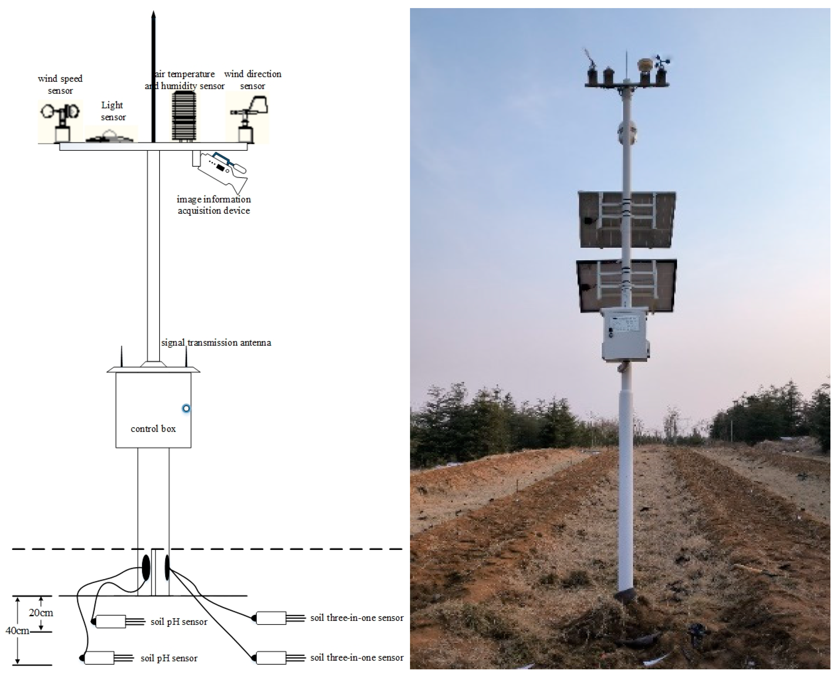
2.1. Experimental Location and Data Sources

The experimental site is located on a Sichuan pepper farm in Laiwu District, Jinan City, Shandong Province, at coordinates 117.48° E longitude and 36.30° N latitude. The area experiences an average annual temperature of approximately 13.0 °C and an average annual precipitation of about 695.3 mm, with rainfall distributed unevenly throughout the year. The experimental data were collected using a fifth-generation IoT environmental information-collection device, independently developed by the laboratory. This device primarily consists of three modules: the sensing terminal module, the sensor module, and the communication module. The connection between the sensing terminal and the sensor devices is established through the ADAM analog acquisition module and RS485 communication interface. The environmental data collected are uploaded to a server-side database via a 4G transmission module, allowing for comprehensive and multi-dimensional monitoring of agricultural environmental information. The dataset includes information such as air temperature, air humidity, light intensity, soil temperature, soil humidity, soil conductivity, and device operating voltage, collected at multiple sites between 18 November 2022, and 18 July 2024, with a collection frequency interval of 5 min. Figure 1 shows the structural diagram and the actual equipment used, and the sensor parameters are listed in

Table 1. Technical parameters of the sensor device.

Sensor Name	Model	Precision	Measurement Range
Air Temperature and Humidity Sensor	DB-171-30	Temperature: ±0.5 °C Humidity: ±5.0% RH	Temperature: (−40~+120) °C Humidity: 0~100% RH
Light Intensity Sensor	TBQ-6	±5%	0.2~200 klux
Soil Temperature, Humidity, and Conductivity 3-in-1 Sensor	TEROS12	Soil Temperature: ±0.1 °C Soil Humidity: ±3% Soil Conductivity: ±5%	Soil Temperature: −40~60 °C Soil Humidity: 1%~100% Soil Conductivity: 0~10 dS/m
Soil pH Sensor	RS-PH-*-TR-1	±5%	3~9 PH
Wind Direction Sensor	RS-FXA-I20	±5%	0~360°
Wind Speed Sensor	RS-FSA-I20	±0.2 m/s	0~60 m/s
Rainfall Sensor	RS-YL-I20-4	±3%	0 mm~4 mm/min

.

2.2. Data Standardization

Data normalization helps eliminate biases caused by differences in the scale or range among data, which can improve the convergence speed of the SVM model, enhance model performance, and reduce biases resulting from differences in feature scales. The normalized sample data of some sensors is shown in

Table 2. Partial sensor normalized sample data.

Air Temperature Normalization	Air Humidity Normalization	Soil Temperature Normalization	Soil Moisture Normalization
0.35	0.62	0.16	0.92
0.31	0.65	0.15	0.90
0.28	0.7	0.14	0.89
0.27	0.68	0.13	0.87
0.25	0.75	0.13	0.85
0.23	0.73	0.12	0.82
0.21	0.78	0.10	0.79

.

$$x^{\prime }={\displaystyle \frac{x-x_{\min }}{x_{\max }-x_{\min }}}$$

(1)

In Equation (1), $x^{\prime }$ represents the normalized data value collected by the sensor, $x$ represents the actual measured value collected by the sensor, $\min$ represents the minimum value in the sample, and $\max$ represents the maximum value.

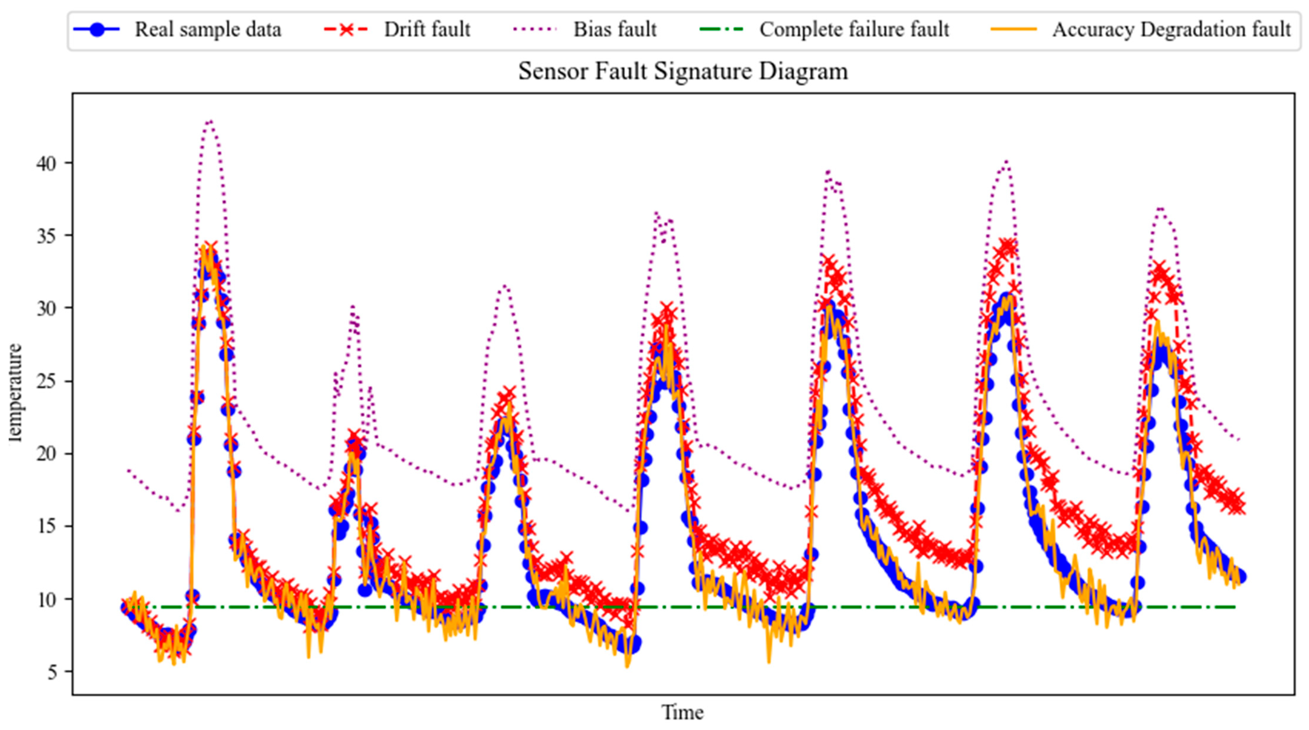
2.3. Theoretical Description of Sensor Faults

In agricultural Internet of Things (AIoT) systems, sensing data are collected from various sensors deployed in agricultural production sites. In the complex agricultural environment, these sensors inevitably encounter multiple fault challenges, including but not limited to complete failure, cumulative fixed bias, drift bias, and gradual degradation in accuracy. Each type of fault poses a challenge to the precise management of agricultural production. By constructing mathematical models of faults and analyzing the underlying mechanisms of sensor failures, a solid foundation can be provided for fault prevention and diagnosis [23]. The standard output expression of a sensor can be defined as

$$x_t=x^{*}(t)+f_t+e_x$$

(2)

In Equation (2), $x_t$ represents the measured value at time $t$ by the sensor node, $x^{*}(t)$ denotes the true value of the data measured at time $t$ and $f_t$ indicates the error introduced at time $t$ due to sensor malfunction. The term $e_x$ represents a random error, typically modeled as a normal distribution with a mean of zero, exhibiting the characteristic bell-shaped curve. That is,

$$e_x~N(0,{\sigma }_1^2)$$

(3)

In Equation (3), ${\sigma }_1^2$ represents the variance of the noise.

2.3.1. Bias Fault

A bias fault is characterized by the sensor consistently producing inaccurate measurement results that deviate from the true value by a fixed amount. For example, if a temperature sensor consistently reads 2 °C higher than the actual temperature, this constitutes a constant bias fault. The causes of such faults often stem from issues like unstable power supply and calibration errors. This type of fault can be defined as

$$x_t=x^{*}(t)+c+e_x$$

(4)

In Equation (4), $c$ is a constant that can vary, representing the difference between the normal value and the faulty value at the same time point.

2.3.2. Drift Fault

A drift fault is characterized by the sensor’s measured value gradually shifting over time, leading to a continuous, unpredictable deviation from the true value. This type of bias may be caused by various factors, with environmental changes being one of the most significant contributors. The mathematical model for a drift fault is given by

$$f_t=z(t-t_m)$$

(5)

In Equation (5), $z$ represents a coefficient, t represents the initial time when the error data appears, and $t_m$ represents any moment when the failure data occurs. Substituting these into Equation (2), the drift failure formula can be defined as

$$x_t=x^{*}(t)+z(t-t_m)+e_x$$

(6)

2.3.3. Accuracy Degradation Fault

An accuracy degradation fault is characterized by the deterioration of a sensor’s measurement capability. This type of fault is typically caused by wear, aging, or damage to the internal components of the sensor. The key feature of this fault is that while the average value of the measurements provided by the sensor remains unchanged, the variance in the measurement results increases, leading to a change in stability and greater dispersion between the measured values. It can be defined as

$$f_t=N(0,{\sigma }_2^2)$$

(7)

In Equation (7), ${\sigma }_2^2$ represents the change in variance. Substituting Equation (7) into Equation (2), since $e_x~N(0,{\sigma }_1^2)$, we obtain

$$x_t=x^{*}(t)+N({\sigma }_2^2+{\sigma }_1^2)$$

(8)

2.3.4. Complete Failure Fault

A complete failure fault represents an extreme condition of sensor malfunction where the measured value no longer changes with the actual measured variable but instead remains at a constant value, typically at its maximum range, such as ‘0’ or another fixed value. This situation is often caused by severe hardware damage, such as circuit disconnection, sensor rupture, or other critical failures. It can be mathematically defined as

$$f_t=\mathrm{m}-x^{*}(t)-e_x$$

(9)

Figure 2 illustrates the waveform characteristics of different fault types using temperature sensor data as an example. The on-site equipment collected temperature sensor data from device 1. On this basis, historical fault data characteristics and added noise were used to simulate the fault data. In the figure, the X-axis represents time (sampling frequency is once every 15 min), and the Y-axis represents temperature (in °C). The blue curve represents the actual data collection (no faults), the red curve represents the drift fault, the purple curve represents the fixed bias fault, the green curve represents the complete failure fault, and the yellow curve represents the accuracy degradation fault. From the analysis of these characteristics, it is evident that accuracy degradation is a gradual process, unlike the abrupt nature of a complete failure fault. This makes accuracy degradation faults more challenging to detect in real time, so diagnosing this type of fault is more complex and difficult.

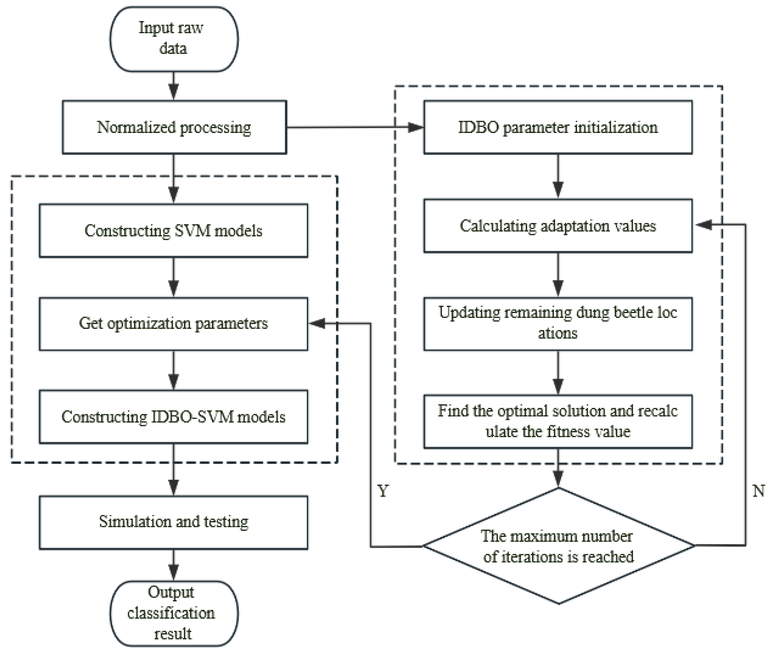
2.4. Construction of Basic Fault Diagnosis Model

2.4.1. SVM (Support Vector Machine) Model

The fault data of agricultural sensors typically exhibit high dimensionality, primarily due to the diversity of sensor types, the high frequency of data collection, and the extraction of various features from the data (such as time-domain and frequency-domain features). Moreover, these data often display significant nonlinear characteristics. Additionally, the low incidence of faults in practical applications results in a typically limited amount of sample data. Against this backdrop, the SVM model demonstrates strong classification capabilities in the field of fault diagnosis. By searching for the optimal hyperplane, it effectively separates different categories of data. The adoption of the structural risk minimization principle allows the model to reduce its sensitivity to noisy data while also minimizing the likelihood of overfitting, thereby enhancing the model’s generalization ability. This is particularly crucial for high-dimensional fault data, as the risk of overfitting is higher in high-dimensional spaces, and data noise can be more challenging to manage. The optimization equation to be solved is

$$\begin{array}{l}min{\displaystyle \frac{1}{2}}||\omega |{|}^2+C{\displaystyle \sum _{i=1}^n{\xi }_i}\\ s.t.y_i(\omega x_i+b)\ge 1-{\xi }_i {\xi }_i\ge 0,i=1,2\cdots ,n\end{array}$$

(10)

In Equation (10), $\omega$ represents the weight vector, ${\xi }_i$ represents the slack variable, $n$ is the sample capacity, and $C$ is a penalty factor that is typically determined by the practical requirements of the fault classification problem. By combining the kernel function with the principle of maximizing the soft margin, and applying the Lagrange multipliers, the classification decision function for the nonlinear Support Vector Machine can be derived, which is expressed as follows:

$$f(x)=\mathrm{sgn}({\displaystyle \sum _{i=1}^n{a}_i}{y}_{i}K(x,x_i)+b)$$

(11)

In Equation (11), $a_i$ represents the Lagrange multiplier, indicating the weight of the support vectors, and satisfies $a_i\ge 0$; $K(x,x_i)$ denotes the kernel function used to project the input sample $x$ and training sample $x_i$ into a high-dimensional space; $y_i$ is the class label of the sample $a_i$; $b$ is the bias term; and $f(x)$ is the classification result for the input sample. To improve the classification accuracy of the SVM, this paper selects the radial basis function (RBF) kernel, which is expressed as

$$K(x,x_i)=\exp (-{\displaystyle \frac{\left|\right|x-x_i|{|}^2}{2{\sigma }^2}})$$

(12)

In Equation (12), $\sigma$ is the parameter of the radial basis function (RBF) kernel. The penalty factor $C$ and the kernel function parameter $\sigma$ are two critical variables that determine classification accuracy. By adjusting the value of $C$, and when using the nonlinear kernel function, it is crucial to enhance classification performance by optimizing the generalization ability of the model. Therefore, it is necessary to optimize these two parameters.

2.4.2. Dung Beetle Optimizer (DBO) Algorithm

The Dung Beetle Optimizer (DBO), proposed by Jianka Xue and Bo Shen in 2022 [24], draws inspiration from various behaviors of dung beetles, such as rolling dung balls, dancing, foraging, and stealing. The algorithm balances global exploration and local exploitation, demonstrating fast convergence and high accuracy in practical applications for classification optimization problems. When a rolling dung beetle moves without obstacles, it adjusts its position based on changes in light intensity, described by the following equation:

$$\begin{array}{l}{x}_i(t+1)=x_i(t)+\alpha \times k\times x_i(t-1)+b\times \Delta x,\\ \Delta x=|x_i(t)-X^{\omega }|\end{array}$$

(13)

In Equation (13), $t$ represents the current iteration number, and $x_i(t)$ represents the position of the $i$ th dung beetle at the $t$-th iteration. The value $b$ is a constant, and $b$ is a random number in the range of (0, 1). The range of $k$ is (0, 0.2], representing the deflection coefficient. $\alpha$ is a natural coefficient used to simulate unexpected situations that may cause deviation from the original direction. The rolling behavior of the dung beetle is simulated using a tangent function to determine the new rolling direction, with the range of the rolling direction limited to [0, π]. The position update formula is as follows:

$$x_i(t+1)=x_i (t)+tan(\theta )\mid x_i (t)-x_i (t-1)\mid$$

(14)

In Equation (14), $\theta$ represents the deflection angle, with a value range of [0, π]. $\mid x_i (t)-x_i (t-1)\mid$ is defined as the deviation of the position of the $i$-th dung beetle during the $t$-th iteration from its position in the previous iteration. The boundary selection strategy is defined as

$$\begin{array}{l}L{b}^{*}=\max (X^{*}\times (1-R),Lb)\\ U{b}^{*}=\min (X^{*}\times (1+R),Ub)\end{array}$$

(15)

In Equation (15), $X^{*}$ represents the local optimal position, $R=1-t/T_{\max }$, where $T_{\max }$ represents the maximum number of iterations. $Lb$ and $Ub$ represent the boundary range, mainly influenced by the value of $R$. Therefore, the dynamic update process of the breeding sphere is defined as follows:

$$B_i (t+1)=X^{*}+b_1\times (B_i (t)-L{b}^{*})+b_2 \times (B_i (t)-U{b}^{*})$$

(16)

In Equation (16), $B_i (t)$ represents the position information of the $i$-th sphere in the $t$-th iteration, while $b_1$ and $b_2$ are random vectors with dimensions of 1 × D, where D represents the dimension of the optimization problem. The position update formula for the dung beetle is as follows:

$$x_i (t+1)=X^b+S\times g\times (|x_i (t)-X^{*}|+|x_i (t)-X^{b }|)$$

(17)

$x_i (t)$ represents the position information of the $i$-th young dung beetle at the $t$-th iteration; $S$ is a constant; and $g$ is a random vector of dimension 1 × D, with a Gaussian distribution characteristic.

2.4.3. Improvements to the Dung Beetle Optimizer (DBO) Algorithm

In-depth exploration reveals that the DBO algorithm exhibits remarkable superiority in its initial applications within foundational comparative experiments. Nevertheless, as problem complexity escalates and the demand for multidimensional optimization intensifies, the inherent limitations of the original DBO algorithm become increasingly pronounced in intricate application scenarios. To surmount these challenges, the DBO algorithm underwent systematic enhancements. By integrating cutting-edge optimization strategies and adaptive mechanisms, its flexibility and robustness were markedly elevated, empowering it to adeptly navigate and excel in complex, dynamic optimization environments.

(1).

Incorporation of Bernoulli Chaotic Map

The Bernoulli chaotic map is a typical chaotic system characterized by sensitivity to initial conditions, periodicity, and ergodicity. The application of chaotic maps in the algorithm aims to utilize their chaotic properties to generate a more uniform and diverse set of initial positions for the population. This can ensure that the population is evenly distributed across the search space, enhancing the algorithm’s global search capability, avoiding local optima, and thereby improving overall optimization performance and convergence speed.

$$Z_{k+1}=\left\{\begin{array}{ll}{\displaystyle \frac{Z_k}{1+\rho }}\hfill & \mathrm{if} Z_k\in (0,1-\rho ]\hfill \\ {\displaystyle \frac{Z_k-1+\rho }{\rho }}\hfill & \mathrm{if} Z_k\in (1-\rho ,1)\hfill \end{array}\right.$$

(18)

Let $Z_k$ represent the current value of the chaotic sequence at the k-th iteration, and $\rho$ the control parameter. When the value of $\rho$ approaches 0.5, the behavior of the chaotic map becomes more complex and unpredictable, leading to a more diverse set of population positions. This helps enhance the exploration ability of the population, enabling the algorithm to more effectively cover the entire search space and avoid premature convergence to local optima. The ergodicity of the optimized chaotic sequence is better manifested, and the numerical changes in the sequence can more uniformly cover the entire possible state space, ensuring sufficient individual searches in different regions and improving overall search efficiency.

(2).

Integration of the Golden Sine Strategy

The position update formula integrating the Golden Sine strategy combines the dynamic characteristics of the sine function with the balancing properties of the golden ratio coefficient, achieving an organic integration of global and local searches. In practical applications, this strategy effectively prevents the algorithm from getting trapped in local optima in high-dimensional complex search spaces and enables the discovery of better solutions within a limited number of iterations. The combination of the sine function and the golden ratio coefficient effectively balances the depth and breadth of the search, enhancing both global and local search capabilities.

$$X_i^{t+1}=X_i^t\times |\sin (R_1)|+R_2\times \sin (R_1)\times |x_1\times P_i^t-x_2\times X_i^t|$$

(19)

$R_1$ is a random number within the range [0, 2π], used to determine the movement distance of an individual; $R_2$ is a random number within the range [0, π], used to determine the direction of an individual’s movement. $x_1$ and $x_2$ represent the weight distribution coefficients, which are used to control the amplitude of the position update.

(3).

Dynamic Weight Strategy Update

The dynamic weight strategy is a critical technique used to balance global exploration and local exploitation during the search and optimization process. By defining the variation rules of two weight coefficients, the search performance of the algorithm is optimized. In the initial iteration stages of the algorithm, the weight coefficient $y_1$ is relatively large, allowing for more intensive searches within the local regions of the solution space, thereby enhancing local exploitation capabilities. This phase of the strategy enables the algorithm to focus on optimizing nearby solutions, reducing the risk of getting trapped in local optima. As the iterations progress, the weight coefficient $y_2$ increases. This adjustment enhances the global search capability of the algorithm, helping it to escape local optima and explore the broader solution space. This dynamic adjustment ensures that the algorithm finds a balance between global exploration and local exploitation. The strategy is defined as follows:

$$\left\{\begin{array}{l}{y}_1=1-{\displaystyle \frac{t^3}{T^3}}\hfill \\ y_2={\displaystyle \frac{t^3}{T^3}}\hfill \end{array}\right.$$

(20)

Here, $t$ represents the current iteration number, and $T$ represents the total number of iterations. This reflects the temporal variation in the weight.

3. Experiment and Result Analysis

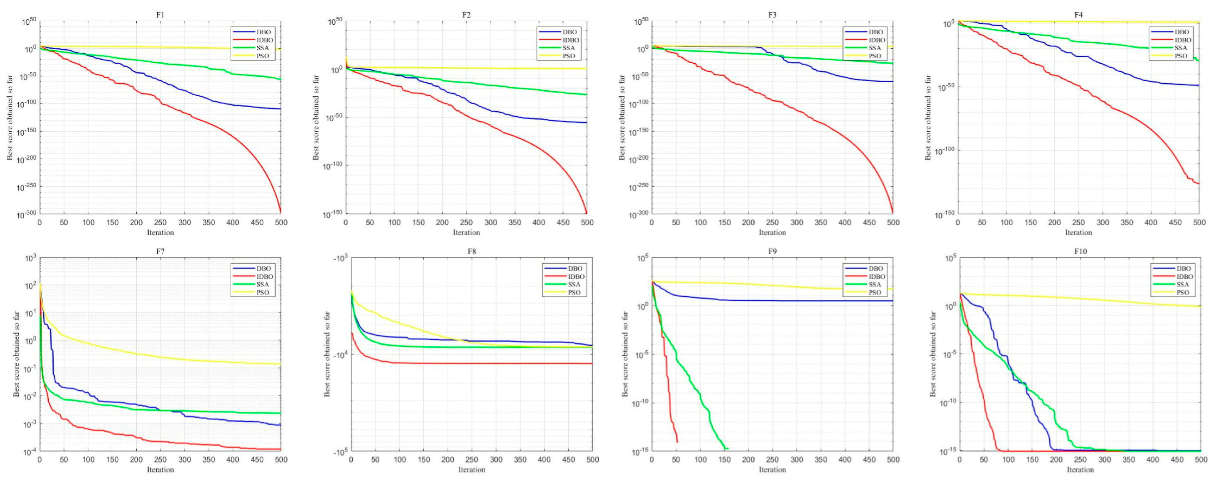
3.1. Performance Testing of the IDBO Algorithm

3.1.1. Performance Comparison Testing of the Improved DBO Algorithm

In this study, the CEC2022 multimodal optimization benchmark function set was used as the primary dataset to evaluate the performance of the model. The CEC2022 benchmark function set is widely employed for assessing the performance of optimization algorithms, particularly in handling complex multimodal optimization problems. This benchmark includes multiple high-dimensional and complex test functions, each with distinct challenging characteristics such as multiple local optima, multimodal issues, and high nonlinearity, making it an ideal tool for evaluating the performance of optimization algorithms in solving complex optimization problems.

The test functions used include F1, F4, and F7 to F10. The characteristics and dimensions of each function are as follows: F1–F4: These functions represent basic single-objective optimization problems with varying dimensions and complexities. F1 and F2 are relatively simple functions, while F3 and F4 contain more local optima. F7–F10: The complexity of these functions is further increased, typically used to test the algorithm’s performance in multimodal optimization problems. These functions contain multiple local optima, challenging the algorithm’s global search capabilities. Specific details of the dataset, such as dimensions, boundary conditions, and the exact form of the objective functions, can be found in the official CEC2022 documentation. To simulate the diverse problems that may be encountered in real-world scenarios, various variants and initial condition settings of these functions were used in the experiments. The specific information concerning the simulation results is shown in

Table 3. Results of IDBO, DBO, SSA, and PSO on the CEC-2022 benchmark functions. The standard deviation is given in parentheses, and the best results are highlighted in bold.

Series of Functions	IDBO	DBO	SSA	PSO
F1 Series	0.00 (0.00)	9.78 × 10−164 (1.02 × 10−110)	9.95 × 10−265 (1.01 × 10−56)	0.00089212 (0.010301)
F2 Series	0.00 (0.00)	1.1507 × 10−88 (4.0265 × 10−48)	2.5063 × 10−109 (1.2556 × 10−31)	0.0015597 (4.4943)
F3 Series	0.00 (0.00)	5.3034 × 10−136 (4.0324 × 10−69)	7.6565 × 10−248 (1.0361 × 10−26)	533.0801 (2480.233)
F4 Series	0 (1.136 × 10−111)	3.1903 × 10−78 (1.9221 × 10−50)	5.1027 × 10−120 (6.4015 × 10−26)	4.769 (1.4015)
F7 Series	1.2809 × 10−5 (0.00011925)	0.00015714 (0.00058625)	6.8396 × 10−5 (0.0020532)	0.024236 (0.49055)
F8 Series	−12569.4865 (1.4191)	−12264.8404 (1948.4593)	−9903.0768 (587.3438)	−9506.6316 (579.1724)
F9 Series	0 (0.00)	0 (22.8855)	0 (0.00)	24.8947 (14.9611)
F10 Series	8.8818 × 10−16 (0)	8.8818 × 10−16 (0)	8.8818 × 10−16 (0)	0.004857 (0.76671)

. The standard deviation (Std Dev) and the mean fitness values are presented to measure the effectiveness of the algorithms in performing the search.

3.1.2. Comparative Analysis of Algorithm Iterative Convergence Curves

The horizontal axis represents the number of iterations of the algorithm, reflecting the convergence speed of each algorithm at different iteration stages. The vertical axis represents the value of the best solution at the current iteration, which typically corresponds to the optimal value of the objective function—the smaller the value, the better the performance of the algorithm.

In all selected test functions, the IDBO (represented by the red curve) demonstrates superior performance, particularly in terms of convergence speed and final convergence value. The IDBO curve descends the fastest and reaches the optimal solution by the final iteration. Whether considering early iteration convergence speed or the final optimal solution achieved, IDBO consistently outperforms the other algorithms. The performance iteration curve of the algorithm is shown in Figure 3.

3.2. IDBO-SVM Fault Diagnosis Model

The penalty factor $C$ in the model is a weight used to adjust the trade-off between classification accuracy and model complexity. As the value of $C$ increases, the training data classification accuracy improves, but it may also lead to smaller classification margins, increasing the likelihood of overfitting and reducing the model’s generalization ability. Conversely, if the $C$ value is too small, it will increase the error classification rate of the training data, resulting in too large a classification margin, which can also reduce the model’s generalization ability.

$g$ is the key hyperparameter that controls the width of the kernel function and directly affects the complexity and generalization ability of the model. Selecting an appropriate $g$ value is crucial for balancing overfitting and underfitting. A smaller $g$ value results in a smoother model, potentially causing underfitting, while a larger $g$ value leads to a more complex model that is prone to overfitting. Additionally, changes in the $g$ value affect the boundary shape between classes and the model’s decision boundary, so it is essential to adjust $g$ experimentally or through other methods to obtain the optimal value. In the training process, to further improve the classification accuracy of SVM, the parameters $C$ and $g$ are taken as the optimization targets, and the SVM classification accuracy is used as the target to find the optimal parameter combination through the foraging behavior of dung beetles. Finally, the optimized SVM model is applied to the test data for classification, and the classification accuracy is compared. The IDBO algorithm is used to search for these two parameters, and the search process is shown in Figure 4.

3.3. Model Performance Evaluation

Based on data standardization, 25,000 consecutive sensor data points were selected as experimental sample data, using four types of data—air temperature, air humidity, soil temperature, and soil moisture—as examples for the experiment. The sample data were split into a training set and a test set in an 8:2 ratio. Referring to the fault characteristics observed in historical sensor data, noise was added to the sample data to simulate fault data, where the fault data were uniformly distributed with a 20% fault ratio and labeled at irregular intervals. Numbers 1 to 5 were used to represent normal values, complete failure, precision degradation failure, drift failure, and constant bias failure, respectively. The labeled and classified dataset was trained and learned using the IDBO-SVM model.

It can be seen from the confusion matrix in Figure 5 that, in the air temperature test dataset, the classification accuracy for normal sample data and complete fault types was 100%. Out of 1000 precision degradation samples, 892 were correctly identified, 91 samples were incorrectly classified as drift faults, and 17 samples were incorrectly predicted as normal. In the drift fault sample data, 845 samples were correctly identified, 117 samples were misclassified as precision degradation faults, and 38 samples were misjudged as normal data. The prediction accuracy for constant bias faults reached 97.30%, with 11 samples incorrectly predicted as normal and 16 samples incorrectly classified as sensor drift faults. The classification accuracy of the model for the air temperature test sample data was 94.20%, 96.98% for the air humidity test samples, 94.46% for the soil temperature test samples, and 95.88% for the soil moisture test samples, demonstrating the effectiveness of the IDBO-SVM model in diagnosing sensor fault data.

3.4. Model Ablation Study

The generalization performance of a model is a key indicator, referring to the model’s ability to maintain good performance on unseen data. To ensure that the proposed IDBO-SVM model can still maintain efficient fault diagnosis capabilities under different sample sizes and fault conditions, it is necessary to rigorously test and validate the model. The ablation experiment aims to systematically alter experimental conditions, particularly the sample size and fault ratio, to analyze and verify the model’s stability and adaptability. By varying the proportion of fault data in the sample set, the model’s performance in handling different levels of fault severity was analyzed to ensure that the model can stably and effectively diagnose sensor faults in practical applications. The experiment was conducted using a newly selected set of 5000 unused sample data points, with a time series interval set to 15 min. Fault ratios of 20% and 30% were set for each group.

From

Table 4. Fault diagnosis model performance comparison.

Model Name	SVM	IDBO-SVM	SSA-SVM	ELMAN	BP
Average accuracy	89.60% (90.60%)	94.20% (95.62%)	91.16% (91.80%)	86.40% (85.26%)	87.66% (87.96%)
Running time	22.5S (21.2S)	18.2S (16.5S)	16.6S (18.7S)	26.6S (22.3S)	31.3S (26.1S)

The bold text indicates the best results.

and Figure 6, it is evident that the performance of the ELMAN and BP neural network models is relatively poor, particularly under the 30% fault ratio, where their accuracy is significantly lower than other models. This indicates that these two neural network models are more sensitive to noise and fault types in the data, lacking a sufficient generalization ability, and are easily disturbed, leading to a notable decline in classification accuracy.

In terms of runtime, the computational efficiency of the ELMAN and BP neural networks is also considerably lower, with the BP model’s runtime reaching as long as 31.3 s. This suggests that when dealing with high-dimensional, high-noise data, the computational overhead for these two models is quite large. The potential reasons could include complex network structures, a large number of iterations, or extra computational load caused by overfitting. This computational cost not only increases training expenses but also further limits the practical application of these models. In contrast, IDBO-SVM demonstrates a higher efficiency and generalization capability, performing more stably in complex environments. Under the 20% fault ratio, the model’s average accuracy is 94.20%, while at the 30% fault ratio, it further improves to 95.62%, the best among all models. Even under different fault ratios and noise conditions, IDBO-SVM is still able to maintain high accuracy, meaning that the model performs well not only on training data but also on test data with higher noise and more complex fault patterns.

In terms of runtime efficiency, IDBO-SVM’s runtime is 18.2 s (20% fault ratio) and 16.5 s (30% fault ratio), demonstrating high efficiency. Although the model has slightly higher computational complexity, its runtime remains relatively short, especially under the 30% fault ratio, where the runtime is even faster than under the 20% fault ratio. This is because, as the fault ratio increases, the IDBO algorithm can converge more quickly to the optimal solution, thus reducing the computation time. The strong adaptability and robustness of the IDBO-SVM model in handling high-noise and complex fault pattern data are attributed to the IDBO algorithm’s ability to effectively optimize the SVM hyperparameters, avoiding local optima and ultimately finding the optimal parameter configuration. This allows the model to maintain good classification performance even with a high noise ratio, further verifying its excellent generalization ability.

4. Conclusions

This study proposes a hybrid model, IDBO-SVM, which optimizes the hyperparameters of the SVM using the IDBO algorithm. It was evaluated for the problem of sensor fault classification under multiple fault types and high-noise conditions. The conclusions are as follows:

(1)

The IDBO algorithm significantly improves the performance of the SVM model by effectively tuning its hyperparameters, especially when handling multimodal data. Compared with other algorithms, IDBO demonstrates faster convergence speed and stronger global search capabilities, enabling it to maintain high classification accuracy even under a high fault ratio. It also shows better computational efficiency, indicating that this model is not only suitable for scenarios requiring high accuracy but also capable of handling real-time application scenarios with high demands on timeliness.

(2)

Ablation experiments show that the robustness and generalization performance of the IDBO-SVM model are outstanding under different fault ratios and sample sizes. Compared to other models, IDBO-SVM excels not only on small sample datasets but also in handling high-fault-ratio data. In practical applications, although sensor data were used in the experiments, it can be inferred that the model also has good adaptability and generalization capabilities in other multimodal fault detection tasks.

As the complexity of sensor networks and fault types increases, there is still room for further improvement. Future research may consider the following directions: Exploring the combination of other global optimization algorithms with machine learning models to further improve the accuracy and real-time performance of fault diagnosis systems. Additionally, investigating how to further optimize the model’s computational performance in scenarios with limited computational resources or higher real-time requirements to meet the demands of more complex industrial settings. Moreover, exploring more methods suitable for sensor fault diagnosis could enhance the accuracy of intelligent decision-making and control systems.

References

1. Goodrich, P.; Betancourt, O.; Arias, A.C.; Zohdi, T. Placement and drone flight path mapping of agricultural soil sensors using machine learning. Comput. Electron. Agric. 2023, 205, 107591. [Google Scholar] [CrossRef]
2. Muangprathub, J.; Boonnam, N.; Kajornkasirat, S.; Lekbangpong, N.; Wanichsombat, A.; Nillaor, P. IoT and agriculture data analysis for smart farm. Comput. Electron. Agric. 2019, 156, 467–474. [Google Scholar] [CrossRef]
3. Maheswararajah, S.; Halgamuge, S.K.; Dassanayake, K.B.; Chapman, D. Management of Orphaned-Nodes in Wireless Sensor Networks for Smart Irrigation Systems. IEEE Trans. Signal Process. 2011, 59, 4909–4922. [Google Scholar] [CrossRef]
4. Zhang, Y.F.; Thorburn, P.J.; Xiang, W.; Fitch, P. SSIM-A Deep Learning Approach for Recovering Missing Time Series Sensor Data. IEEE Internet Things J. 2019, 6, 6618–6628. [Google Scholar] [CrossRef]
5. Bae, J.; Lee, M.; Shin, C. A Data-Based Fault-Detection Model for Wireless Sensor Networks. Sustainability 2019, 11, 6171. [Google Scholar] [CrossRef]
6. Bhardwaj, A.; Kumar, M.; Alshehri, M.; Keshta, I.; Abugabah, A.; Sharma, S.K. Smart water management framework for irrigation in agriculture. Environ. Technol. 2024, 45, 2320–2334. [Google Scholar] [CrossRef]
7. Kaur, G.; Bhattacharya, M. Intelligent Fault Diagnosis for AIT-Based Smart Farming Applications. IEEE Sens. J. 2023, 23, 28261–28269. [Google Scholar] [CrossRef]
8. Rahaman, M.M.; Azharuddin, M. Wireless sensor networks in agriculture through machine learning: A survey. Comput. Electron. Agric. 2022, 197, 106928. [Google Scholar] [CrossRef]
9. Erhan, L.; Ndubuaku, M.; Di Mauro, M.; Song, W.; Chen, M.; Fortino, G.; Bagdasar, O.; Liotta, A. Smart anomaly detection in sensor systems: A multi-perspective review. Inf. Fusion 2021, 67, 64–79. [Google Scholar] [CrossRef]
10. Purbowaskito, W.; Lan, C.Y.; Fuh, K. The Potentiality of Integrating Model-Based Residuals and Machine-Learning Classifiers: An Induction Motor Fault Diagnosis Case. IEEE Trans. Ind. Inform. 2024, 20, 2822–2832. [Google Scholar] [CrossRef]
11. Saeed, U.; Lee, Y.D.; Jan, S.U.; Koo, I. CAFD: Context-Aware Fault Diagnostic Scheme towards Sensor Faults Utilizing Machine Learning. Sensors 2021, 21, 617. [Google Scholar] [CrossRef] [PubMed]
12. Li, C.; Shen, Q.; Wang, L.X.; Qin, W.W.; Xie, M.M. A New Adaptive Interpretable Fault Diagnosis Model for Complex System Based on Belief Rule Base. IEEE Trans. Instrum. Meas. 2022, 71, 3529111. [Google Scholar] [CrossRef]
13. Zou, X.G.; Liu, W.C.; Huo, Z.Q.; Wang, S.Y.; Chen, Z.L.; Xin, C.R.; Bai, Y.A.; Liang, Z.Y.; Gong, Y.; Qian, Y.; et al. Current Status and Prospects of Research on Sensor Fault Diagnosis of Agricultural Internet of Things. Sensors 2023, 23, 2528. [Google Scholar] [CrossRef] [PubMed]
14. Hao, H.Y.; Zhang, K.; Ding, S.X.; Chen, Z.W.; Lei, Y.G. A data-driven multiplicative fault diagnosis approach for automation processes. Isa Trans. 2014, 53, 1436–1445. [Google Scholar] [CrossRef]
15. Nor, N.M.; Hassan, C.R.C.; Hussain, M.A. A review of data-driven fault detection and diagnosis methods: Applications in chemical process systems. Rev. Chem. Eng. 2020, 36, 513–553. [Google Scholar] [CrossRef]
16. Liakos, K.G.; Busato, P.; Moshou, D.; Pearson, S.; Bochtis, D. Machine Learning in Agriculture: A Review. Sensors 2018, 18, 2674. [Google Scholar] [CrossRef]
17. Foo, L.K.; Chua, S.L.; Ibrahim, N. Attribute Weighted Naive Bayes Classifier. Cmc-Comput. Mater. Contin. 2022, 71, 1945–1957. [Google Scholar] [CrossRef]
18. Kamilaris, A.; Prenafeta-Boldú, F.X. Deep learning in agriculture: A survey. Comput. Electron. Agric. 2018, 147, 70–90. [Google Scholar] [CrossRef]
19. Kari, T.; Gao, W.S.; Zhao, D.B.; Abiderexiti, K.; Mo, W.X.; Wang, Y.; Luan, L. Hybrid feature selection approach for power transformer fault diagnosis based on support vector machine and genetic algorithm. Iet Gener. Transm. Distrib. 2018, 12, 5672–5680. [Google Scholar] [CrossRef]
20. Maincer, D.; Benmahamed, Y.; Mansour, M.; Alharthi, M.; Ghonein, S.S.M. Fault Diagnosis in Robot Manipulators Using SVM and KNN. Intell. Autom. Soft Comput. 2023, 35, 1957–1969. [Google Scholar] [CrossRef]
21. Ye, L.; Chen, Z.; Liu, J.; Lin, C.; Jian, Y. Research on Power Device Fault Prediction of Rod Control Power Cabinet Based on Improved Dung Beetle Optimization-Temporal Convolutional Network Transfer Learning Model. Energies 2024, 17, 447. [Google Scholar] [CrossRef]
22. Huang, H.; Yao, Z.; Wei, X.; Zhou, Y. Twin support vector machines based on chaotic mapping dung beetle optimization algorithm. J. Comput. Des. Eng. 2024, 11, 101–110. [Google Scholar] [CrossRef]
23. Sharifi, R.; Langari, R. Isolability of faults in sensor fault diagnosis. Mech. Syst. Signal Process. 2011, 25, 2733–2744. [Google Scholar] [CrossRef]
24. Xue, J.K.; Shen, B. Dung beetle optimizer: A new meta-heuristic algorithm for global optimization. J. Supercomput. 2023, 79, 7305–7336. [Google Scholar] [CrossRef]
Figure 1. IoT sensing device.
Sustainability 16 10001 g001
Figure 2. Sensor fault waveform characteristics diagram.
Sustainability 16 10001 g002
Figure 3. Performance comparison chart of optimization algorithms.
Sustainability 16 10001 g003
Figure 4. IDBO-SVM troubleshooting flow.
Sustainability 16 10001 g004
Figure 5. (a) Confusion matrix for classification of temperature sensor fault prediction. (b) Confusion matrix for classification of humidity sensor fault prediction. (c) Confusion matrix for classification of soil temperature sensor fault prediction. (d) Confusion matrix for classification of soil humidity sensor fault prediction.
Sustainability 16 10001 g005
Figure 6. Fault diagnosis model accuracy comparison.
Sustainability 16 10001 g006