Abstract
Traffic emissions pose a substantial challenge for contemporary societies, particularly at roundabouts, where high levels of vehicle interaction and the associated emission dynamics are prevalent. Building upon this, a cellular automata model was developed to simulate traffic characteristics, including fuel consumption, emissions (CO, HC, and NOx), and vehicle speed at a large roundabout. The model examines critical parameters, such as interaction, stop-and-go behavior, density, speed, and spacing, to identify the factors influencing fuel consumption and emissions in roundabout traffic. Numerical verification confirmed the model’s effectiveness in replicating complex traffic flows at large roundabouts, while also revealing that driving behavior, particularly during lane entry, is a critical factor influencing fuel consumption and emissions. Therefore, we proposed four optimization strategies—two space-based and two behavior-based—aimed at reducing emissions and enhancing traffic efficiency. Simulation results demonstrated that the behavior-based strategies achieved reductions of up to 18.40%, 43.20%, 28.98%, and 30.02% in fuel consumption and emissions, along with an 8.88% increase in traffic efficiency. In contrast, the space-based strategies improved traffic efficiency by 10.26%, while reducing fuel consumption and emissions by 8.25%, 32.64%, 18.48%, and 18.09%. While the space-based strategies enhanced traffic efficiency more, their overall optimization effects were relatively modest. Thus, integrating these strategies can enhance roundabout traffic efficiency across varying conditions, while reducing fuel consumption and emissions. These findings can enhance our understanding of the traffic parameters affecting vehicular emissions, offering crucial insights for urban planners and policymakers to optimize roundabout design and management toward greater sustainability and environmental benefits.
1. Introduction
Vehicular traffic is widely recognized as a major contributor to issues such as congestion, traffic accidents, and environmental pollution. In alignment with the United Nations Sustainable Development Goals (SDGs), reducing greenhouse gas concentrations is critical to achieving net-zero emissions. Recently, vehicular emissions have become a critical environmental issue [1,2]. Hoek et al. [3] studied the relationship between fine particulate matter (PM2.5) and cardiovascular and respiratory mortality among adults in 337 cities. They found that a 10 μg/m3 increase in monthly PM2.5 was associated with an increase of 1.3% in cardiovascular mortality and a 0.9% increase in respiratory mortality.
Vehicle emissions intensify at intersections, due to frequent deceleration, acceleration, and idling, resulting in significant variability in vehicle speeds. Intersections come in various forms, such as roundabouts, unsignalized intersections, and signalized intersections. Under light traffic conditions, roundabouts generally exhibit superior performance. Beyond improving traffic flow and safety, roundabouts serve as city landmarks, help structure urban landscapes, and provide a sense of subjective safety for drivers, pedestrians, and cyclists, as recent studies have indicated [4,5]. Nonetheless, roundabouts can still be substantial sources of urban traffic emissions [6]. Meneguzzer et al. [7,8] compared emissions from signalized intersections and roundabouts. They discovered that replacing traffic signals with roundabouts tends to reduce CO2 emissions, although the differences are not always statistically significant. Conversely, signalized intersections tend to perform better regarding NOx emissions. Additionally, they observed that driver behavior has a substantial impact on pollutant emissions, a finding corroborated by Hallmark et al. [9] in their study.
In this context, significant research has been dedicated to investigating fuel consumption and vehicular emissions [10,11,12]. Numerous traffic flow models have been developed to evaluate and predict traffic-related emissions in real life [13,14,15]. However, a significant limitation of these models is their failure to account for instantaneous speed fluctuations, which critically affect vehicular emissions in real traffic conditions. Similarly, individual vehicle interactions play a crucial role in determining overall traffic efficiency and emissions. Just as microstructural properties influence macroscopic performance in materials through causal emergence, the localized movement patterns of vehicles within a roundabout give rise to emergent behaviors that significantly impact the broader traffic dynamics [16,17,18,19]. To address these complexities, extensive research has focused on employing microscopic traffic flow models that account for instantaneous speed fluctuations to more accurately calculate vehicular emissions [20,21,22]. Therefore, understanding the patterns of vehicle movement within roundabouts and how these movements contribute to emissions is crucial for developing strategies to mitigate these effects.
Currently, researchers use two main approaches to study these issues: experiments, which capture real-world vehicle behavior and emissions data; and simulations, which can replicate a wide range of traffic scenarios to analyze emissions under different conditions. For example, empirical studies on the effect of vehicle behavior (e.g., gap-acceptance behavior, and aggressive driving behavior, etc.) on roundabout traffic flow have been conducted, aiming to establish a reliable experimental basis for proposing, validating, and evaluating corresponding traffic flow models [23,24,25,26]; the variations in vehicle behavior depending on different positions in a roundabout (e.g., entrance, exit, etc.), as well as across different types of roundabouts (e.g., multi-lane roundabouts, and turbo roundabouts, etc.), have also been explored [27,28,29,30]. Fernandes et al. [31], based on empirical research, developed a traffic flow model for roundabouts and compared the emissions of vehicles moving through turbo roundabouts with those through conventional multilane roundabouts. Their findings indicated that vehicles at turbo roundabouts generate more emissions (15–22%, depending on the pollutant) compared to multilane conventional roundabouts, particularly under medium to high congestion levels. Lakouari et al. [32] modeled roundabouts and found that CO2 emissions are closely related to both traffic signals and vehicle injection rates. Bahmankhah et al. [33,34] conducted empirical research and modeling on single-lane (SL), compact two-lane (CTL), and multi-lane (ML) roundabouts. They found a strong relationship between conflict frequency, emissions, and roundabout type, with ML roundabouts exhibiting the highest conflict frequency, which results in higher emissions. Wang et al. [35] conducted a study on the ML roundabout at Satellite Square in Changchun, focusing on congestion and emissions. They proposed optimization strategies based on traffic signal control, which led to reductions in emissions of CO by 10.20%, HC by 12.22%, and NOx by 7.44%. Małecki et al. [36] presented a realistic vehicle braking phase, tailored to the type of vehicle and weather conditions, and examined the capacity of multi-lane roundabouts under various road traffic rules.
Numerous models have been developed to address various traffic-related issues, incorporating nonlinear factors that characterize complex traffic systems [37,38,39,40,41,42,43,44,45,46,47]. Cellular automata (CA) models have been extensively utilized in microscopic traffic simulations to effectively replicate vehicle decision-making behavior. In such CA-based research, the road network, time, and vehicle velocities are discretized, with each cell’s state updated based on predefined rules, leading to dynamic evolution of the system.
CA models have been employed to investigate traffic emissions, offering insights into emission patterns and dynamics, Marzoug et al. [48] investigated traffic emissions at conventional traffic lights, double traffic lights, and self-organizing intersections. They proposed two strategies, which reduced traffic emissions by 13.6% and 3.6%, respectively. Wang et al. [45] studied traffic emissions using cellular automata models and a mixed NaSch traffic flow model. They found that the maximum speed of short vehicles has a significant impact on emissions when the mixing ratio and length of vehicles are fixed. Qiao et al. [49] studied particulate matter (PM) emissions from two typical cellular automata traffic models (VDR and TT models) with slow-to-start rules, under both periodic and open boundary conditions. For periodic boundary systems, the initial conditions significantly influenced the formation of traffic congestion and PM emissions. In contrast, for open boundary systems, the exit probability played a major role in both traffic congestion and particulate emissions. Lakouari et al. [32] proposed a cellular automaton model to describe driver behavior at a single-lane urban roundabout and investigated the differences in emissions between single-lane roundabouts and signalized intersections.
Many traffic flow models developed for roundabouts lack a focus on vehicular emissions, and the literature indicates limited applications of cellular automata (CA) to model such emissions [50]. In many studies, roundabouts are often simplified as four-way intersections. However, large real-world roundabouts, due to their extended travel distances and frequent vehicle interactions, are more prone to excessive fuel consumption and emissions. These characteristics significantly impact traffic dynamics and emissions, especially for large roundabouts. This paper presents several innovations that fill this research gap regarding fuel consumption and emissions in complex traffic systems at large roundabouts:
- A roundabout traffic flow model is proposed to replicate the complex interactions between vehicles at large roundabouts, by simulating three stages of entrance, following, and exit.
- A multi-lane vehicle motion model for large roundabouts was developed.
- A study was conducted on the fuel consumption and emissions of traffic flow of large roundabouts.
- Multiple optimization strategies for fuel consumption and emissions were proposed, based on the spatial and vehicular behavior characteristics of large roundabouts.
The objective of this study was to develop a model that accurately replicates the complex traffic flow dynamics of large roundabouts. It aimed to assess the influence of driving behavior on fuel consumption and emissions, focusing on how these behaviors affect overall traffic efficiency. Furthermore, the study sought to propose and evaluate optimization strategies to enhance traffic efficiency, while minimizing fuel consumption and emissions. This model is grounded in empirical research conducted at the Guanggu Roundabout in Wuhan.
The structure of this paper is as follows: Section 2 discusses the construction of the roundabout traffic flow model, including driving behavior, fuel consumption, and emission models. Section 3 covers the validation of the model’s effectiveness, proposing optimization strategies based on the issues identified. Section 4 presents and discusses the analysis results. Section 5 provides the conclusions.
2. Model
The model in this paper was constructed based on empirical observations of objective patterns and traffic rules. Therefore, this section includes the study of roundabouts, the development of movement models, and the formulation of fuel consumption and emission models.
2.1. Empirical Observation
To analyze the operational characteristics of traffic flow within a complex roundabout environment, we conducted a field study at the Guanggu Roundabout in Wuhan, China (see Figure 1a). This roundabout features four concentric lanes (R1 to R4, from the innermost to the outermost) and connects to the external traffic network via several radial roads. For ease of reference, we have labeled these radial roads A through F in a counterclockwise direction. Each road includes both entrance and exit branches. Based on Google Maps, we outlined the geometry of the roundabout, as illustrated in Figure 1b. The lanes, R1 through R4, each have a width of 3.6 m and circumferences of 514 m, 536 m, 559 m, and 581 m, respectively. Roads F and B each have one lane for both entrance and exit, while the other radial roads feature two lanes for their entrances and exits. To accurately depict the locations of the entrances and exits relative to the roundabout, we recorded the latitude and longitude of specific calibration points, characterized by distinct features such as the start and end points of channelizing islands and the intersection points of R4 with Roads A–F (Figure 1b). Our study focused on the inner area of the roundabout and the sections of the radial roads close to their entry and exit points.
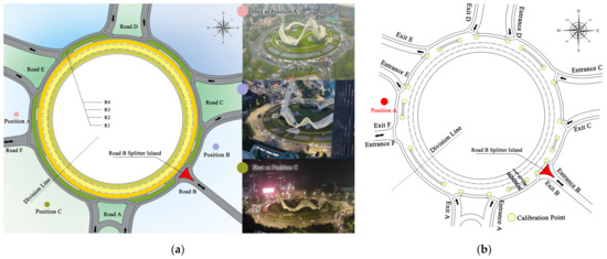
Figure 1.
(a) Snapshot and video recording positions of the Guanggu Roundabout: (b) schematic sketch providing spatial information based on (a).
We set up three monitors around the roundabout and selected Position A (monitor details: brand: Canon 6D Mark II; resolution: 1080P; fps: 25), which had the least obstruction and provided the clearest view. The observation period spanned from 2:12:32 p.m. to 2:32:32 p.m. on 11 November 2023, totaling 1200 s. During this period, 1507 vehicles traversed the roundabout, displaying regular driving behaviors that formed the basis of our empirical analysis:
- When vehicles enter the roundabout, their choice of lane (R1–R4) is closely correlated with their target exit. The lane selection probabilities are presented in Figure 2.
- Vehicle movement within the roundabout is divided into three stages: the entrance stage, the following stage, and the exit stage. The decision-making behavior of vehicles varies across these stages.
The Entrance Stage (Stage 1):
- 3.
- As vehicles prepare to enter the roundabout, they exhibit yielding behavior toward vehicles already circulating within it. The distance at which yielding occurs is related to the lane (R1–R4) in which the internal vehicles are located.
- 4.
- Vehicles in this stage aim to reach their target lane through continuous lane changes. When positioned in R2, completing lane changes requires longer distances due to the higher speeds of other vehicles.
- 5.
- When two vehicles are side by side at the entrance and share the same target position, the vehicle on the right has priority in proceeding first.
The Following Stage (Stage 2):
- 6.
- In this stage, vehicles tend to maintain their maximum speed and avoid changing lanes unless congestion occurs, in which case they may choose to move outward (farther from the center of the roundabout).
- 7.
- In the innermost lane (R1), if there is one radial road remaining to the target exit, the majority of vehicles (about 86%) will choose to move outward to lane (R2); otherwise, they continue forward until reaching the exit area.
The Exit Stage (Stage 3):
- 8.
- Vehicles in this stage aim to reach the exit through continuous lane changes, but lane-changing behavior is significantly influenced by other vehicles, especially when positioned in lanes R1 and R2, where the distance required for lane changes is greater.
- 9.
- Vehicles in the outer lanes can prioritize lane changes more effectively compared to those in the inner lanes, particularly when competing for the same position.
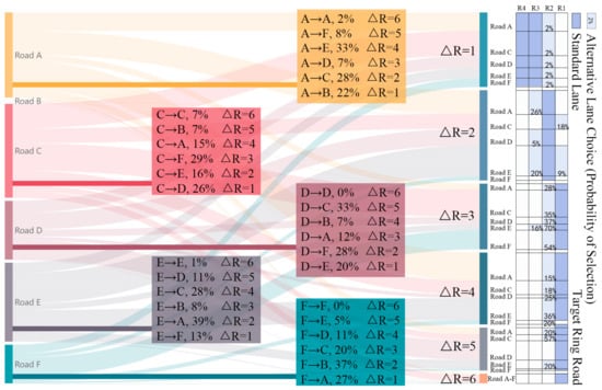
Figure 2.
Choice probability based on empirical observations. The left side of the figure illustrates the probability distribution of vehicles’ start and end roads, while the right side shows the probability of lane choices within the roundabout when entering from different entrances (A–F).
Although insightful, these observations alone cannot replicate the complex interactions in roundabouts or adequately support testing of flow-enhancing strategies and analysis of fuel consumption and emissions. Therefore, we focused on developing a more broadly applicable model based on these findings.
2.2. Vehicle Movement
To describe vehicle movement in the system, we adopted the Nagel–Schreckenberg (NaSch) model, a stochastic cellular automata model where space and time are discretized [51].
2.2.1. Conversion of the Roundabout into a Modeling Scenario
We transformed the roundabout into a rectangular grid, with cells uniformly distributed across each lane. Due to the varying perimeters of the lanes—shorter near the center—the cell lengths differed across road segments. To ensure consistency between the actual roundabout and the simulation, we used the cells from lane R3 (559 m) as the standard. This lane was divided into 155 cells, each 3.6 m long. Consequently, the cell lengths for lanes R1 (514 m), R2 (536 m), and R4 (581 m) were adjusted to 3.32 m, 3.46 m, and 3.75 m, respectively. The simulation base map was configured as a 5 × 155 matrix, with each lane represented by 155 cells, corresponding to matrix columns. The four lanes (R1–R4) corresponded directly to Rows 1 through 4 in the matrix, with the exit–entrance row represented as Row 5. Together, these five rows formed the base map matrix (Figure 3).
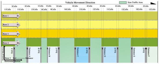
Figure 3.
Unfolding of the roundabout.
2.2.2. General Rule of Vehicle Motion
We developed a sequential update algorithm with a priority order, to manage the system and vehicle updates. In terms of priority, if vehicles are scheduled to occupy the same position at the same update time, those in the following stage take precedence. If both vehicles have the same priority, the order of their updates is determined randomly.
Here, we abstract the roundabout into a complex traffic system where vehicles discretely update and interact with each other. The specific rules are as follows:
- Vehicles cannot overlap in space.
- Vehicles are categorized into fast (3 cells/s) and slow (2 cells/s) types. In the map, vehicles occupying two cells. The injection rate at each entry matches actual observations (0.75 s per vehicle).
- Vehicle movement is categorized into three stages based on motion rules and position: entrance, following, and exit stages.
- Based on the range of influence of a vehicle’s lane change, the lane-changing maneuver involves both vertical and horizontal movements (Figure 4). Four adjacent cells will be impacted, and no other vehicles can occupy these cells while the lane-change process is being executed.
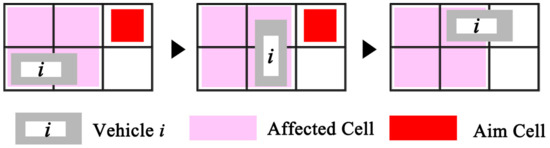 Figure 4. Lane-changing steps.
 - Each lattice represents a cell that is either vacant or occupied at any given moment. For vehicle movement, each time step is divided into two phases: the first phase involves applying the movement model to make decisions (i.e., updating the vehicle’s position), while the second phase calculates the vehicle’s subsequent update time.
- All vehicles move based on the sequential update algorithm. The simulation time step was set to 0.01 s, and the total steps were 120,000.
Due to the differing cell lengths of each lane, the traditional NaSch model was not effective in addressing this issue [52]. Based on the research by Gier et al. [53], we integrated driving decision-making behavior with the NaSch model. Vehicles are restricted to move a maximum of one cell per update. In this context, the vehicle’s speed (cell/s) is represented by the update frequency (δ, s): a higher update frequency corresponds to a higher speed. Therefore, once the i-th vehicle has completed its movement update at update time (t), the system calculates the time interval (i.e., the update frequency ) required for the next update based on the current speed vi(t). Simultaneously, the NaSch model is used to determine the speed for the next update time (t + ).
The update frequency formula is as follows:
where vi(t) is the speed of the i-th vehicle at time (t), and is the update frequency of the i-th vehicle for the next update. The values of k are 0.92 (vehicle in R1), 0.96 (vehicle in R2), 1.00 (vehicle in R3), and 1.04 (vehicle in R4), reflecting the ratio of the cell lengths in different lanes (e.g., a shorter cell length in R1, hence k = 0.92). In the case of vertical movement, the cell length is 3.6 m, with k = 1.
The speed of the next update time is calculated by the three rules of the NaSch model:
- Acceleration: .
- Deceleration: .
- Randomization: , with a braking probability p.
where and denote the maximum speed and the number of empty cells in front of the i-th vehicle, respectively (Figure 5). The determination of braking probability p was referenced from the study by Li et al. [23]. Subsequently, the i-th vehicle is updated at time (t + ).
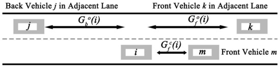
Figure 5.
Variable related to vehicle behavior.
and denote the number of empty cells in front of and behind the i-th vehicle in the adjacent lane, respectively.
2.2.3. Vehicle Motion in Three Stages
During the entrance stage (stage 1), vehicles prioritize lane-changing maneuvers until they enter the target lane, then they transition to the following stage. Before vehicles enter the roundabout from the entry cell, they need to assess the horizontal distance between the vehicle and those circulating normally within the roundabout. This distance varies depending on the lane, with lengths of 4 cells (in R3), 6 cells (in R2), and 7 cells (in R1), respectively, (case 1 in Figure 6) R4 is not considered in this case. If there are other vehicles within the distance in any lane between the vehicle and the target lane, the vehicle must wait. Vehicles entering from the entry cell proceed to lane R4 and navigate within the buffer zone (indicated by the yellow area in Figure 6) during the entrance stage. represents the length of the buffer zone across different lanes. In the case of a dual-lane entrance, is as follows: 7 cells (in R2), 4 cells (in R3), and 3 cells (in R4); for single-lane entrance, the number is decreased by 1. The buffer zone position is determined by the left boundary (shown as the red line in Figure 6). After a vehicle has completed a lane change into R2 with R1 as its target lane, it must move at least one cell horizontally before attempting another lane change at the next update time (as shown in case 2, Figure 6).
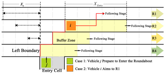
Figure 6.
Vehicle movement during the entrance stage.
Before processing a vertical movement for a lane change, the distances and must exceed (the maximum speed of the j-th vehicle, Figure 5) and 3 cells, respectively. Lane-changing will not be chosen if the adjacent cell in the other lane is occupied.
During the following stage (stage 2), the vehicle will primarily move horizontally. If a vehicle remains stationary for two consecutive updates (an indication of congestion) the probability of a lane change is determined as follows: for vehicles in R1, there is a 60% chance of changing lanes; for those in R2, there is a 45% chance, with a 5% likelihood of moving to R1 and a 40% likelihood of moving to R3. Vehicles in R3 or R4 will remain in their current lanes. Specifically, if a vehicle in R1 passes the advanced lane-changing cell (the green block in Figure 7), there is an 86% probability that it will switch to R2 in subsequent movements; otherwise, it will continue straight towards the exit area (Figure 7).
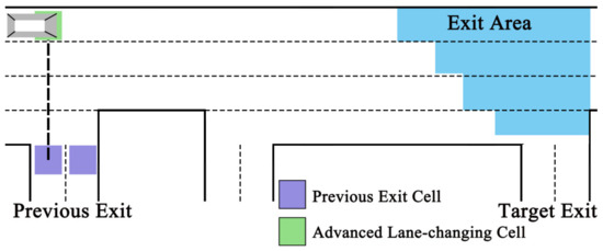
Figure 7.
Vehicle movement during the following stage.
During the exit stage (stage 3), vehicles prioritize lane-changing maneuvers until they enter the exit cell. When a vehicle enters the checkpoint, it then moves within the buffer zone (shown as the yellow area in Figure 8). Similarly, is the cell number of the buffer zone in different lanes, for a dual-lane exit, with values as follows: 10 cells (in R1), 7 cells (in R2), 5 cells (in R3), and 3 cells (in R4); for a single-lane exit, this number is decreased by 1. The position of the buffer zone is determined by the right boundary (shown as the red line in Figure 8). The checkpoint is the left boundary of the buffer zone in a different lane. When vehicles change lanes towards the exit from R1 or R2, they must move horizontally at least 2 cells after completing a lane change before they can change lanes again (shown as the i-th vehicle in Figure 8).
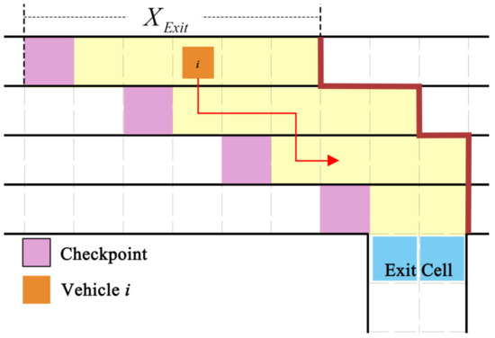
Figure 8.
Vehicle movement during the exit stage.
Once a vehicle reaches the exit cell, it is removed from the system.
2.3. Vehicle Emissions and Fuel Consumption
Over the past century, various models for fuel consumption and emissions in traffic systems have been developed [54,55,56,57]. Among these, the VT-Micro model [54,55,58] stands out for estimating fuel consumption and emissions based on a vehicle’s instantaneous speed and acceleration. However, this model presents limitations when incorporating electric vehicles (EVs) into modern urban traffic systems. Although EVs are becoming more prevalent in cities, a survey conducted in Wuhan revealed that EVs only account for 7% of the total vehicle population [59]. For simplicity and to facilitate effective feedback for optimization strategies, this study assumed all vehicles were fuel-powered. This assumption streamlined the calculations and analysis within the context of fuel consumption and emissions. Regarding parameter selection, this study referenced the work of Tang et al. [60], who employed a similar modeling approach to examine the impact of small traffic flow perturbations on fuel consumption and emissions. Their research provides a robust basis for parameterizing the VT-Micro model, ensuring that the optimization strategies yield accurate and validated results for fuel consumption and emissions. Therefore, this paper utilized the VT-Micro model to calculate fuel consumption and emissions within the traffic system. The model can be described as follows:
where is the fuel consumption and emission rate of each vehicle. i and j are the exponential coefficients of speed and acceleration , respectively. is the regression coefficient under the power i of speed and the power j of acceleration (Table 1). The algorithm retrieves the actual speed closest to the start and end of each second (speed from the movement model multiplied by the length of the cell the vehicle occupies, m/s) every second, with representing the difference in speed between the start and end of each second and set to 1.

Table 1.
The regression coefficient in Equation (2). Input: speed (m/s), acceleration (m/s²); output: fuel consumption (mL/s), emissions (CO, HC, NOx) (mg/s).
3. Validation of the Model and Optimization Strategies
We validated the effectiveness and identified factors affecting vehicle fuel consumption and emissions based on simulation results and real-world conditions. We proposed four targeted optimization strategies.
3.1. Validation
In this section, two indicators were adopted to compare the model output with the empirical study: (1) a fundamental diagram, which is one of the most characteristic features in roundabout traffic flow studies; and (2) the variation in the outflow number over time.
3.1.1. Fundamental Diagram
A ‘Fundamental Diagram’ is derived from the ratio of effective vehicle speed to density, reflecting roundabout efficiency. Due to the circular nature of the driving route, calculating speed and density is challenging. Therefore, we established a typical trajectory to quantify the vehicle trajectories. Specifically, the typical trajectory represented the vertical projection of a vehicle’s actual movement trajectory within the roundabout onto its target lane (Figure 9).
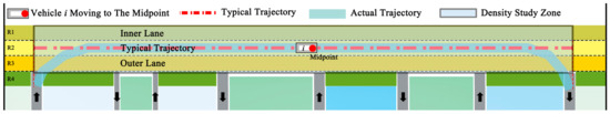
Figure 9.
Typical trajectory.
For each vehicle, the effective speed is defined by the length of the typical trajectory and the total duration of each vehicle within the system, that is
For density analysis, we focused on the density study zone, which consists of the inner lane, a typical trajectory, and the outer lane (Figure 9). The density D is defined as the ratio of the total vehicle area , to the total area of the zone , as follows:
where the total vehicle area represents the area occupied by all vehicles within the density study zone when the i-th vehicle reaches the midpoint of the typical trajectory.
The results are shown in Figure 10. It can be noted that the data values extracted from empirical research (gray line) closely approximate those in the simulation (red line). As density increased, the effective speed decreased in a similar manner. In high-density situations, the consistency between the two curves is more satisfactory. However, at lower densities, slight differences can be observed between the simulation data and empirical research, although the overall consistency remains strong. We found that sample sizes for densities between 0 and 0.06 and above 0.33 were too small to be statistically significant. Therefore, for the purpose of this study, we defined a density range of 0.06–0.33 as the focus of our analysis.
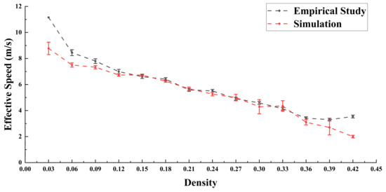
Figure 10.
Fundamental diagram (density is the ratio of the area occupied by vehicles to the area of the density study region (m2/m2)).
3.1.2. Relationship Between Traffic Flow and Time
We present the temporal evolution of the data on vehicles exiting the roundabout in both the empirical research and simulation, data were recorded at 10 s intervals (Figure 11a). It can be observed that the changes in the number of vehicles within the observation area were remarkably similar under the same input conditions. The peaks of both curves are identical and occurred at almost the same time. Anomalous fluctuations occurred at 530–550, 970, and 1150, but normal conditions were quickly restored. To assess the impact of these anomalies, we compiled and accumulated data on vehicle exits from the simulated roundabout every 10 s, as well as entry and exit data from the empirical study, for analysis (Figure 11b). A Pearson test was conducted to examine the statistical correlation between the cumulative traffic flow data from the empirical research and simulation, revealing a significant correlation (p < 0.05) with a strong positive relationship (Pearson correlation ≈ 1).
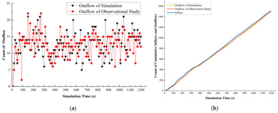
Figure 11.
Schemes of the number of outflows. (a) Count of vehicles exiting the roundabout at a fixed interval (10 s); (b) cumulative inflows and outflows.
Validation of the model’s effectiveness is now complete, based on both the fundamental diagram and the variation in outflow numbers over time. This indicates that the model can accurately replicate traffic conditions within the roundabout, providing a feasible foundation for subsequent research on fuel consumption and emissions.
3.2. Analysis of Influencing Factors
Significant research has focused on traffic emissions based on driving behavior, highlighting that stop-and-go behavior substantially impacts emissions [61,62,63]. For instance, Coelho et al. [64] modeled a single-lane roundabout based on empirical data and found that stop-and-go behavior significantly affects emissions, hypothesizing that this is related to traffic flow conflicts. Similarly, Lakouari et al. [32] focused their research on traffic behavior and emissions before entering a roundabout, as well as on the lanes leading out of the roundabout. However, their studies did not address the micro-level relationship between traffic behavior and emissions within a roundabout, which is the primary focus of this paper.
Therefore, we first examined the occurrence of vehicle interactions and stop-and-go behavior at three different stages (Figure 12). Interaction behavior is defined as recording an interaction whenever a vehicle changes lanes and there are other vehicles present within the neighboring five cells. For each vehicle, a stop-and-go behavior was recorded when it experienced a stop and then a restart. The final analysis considered the density levels of the occurrence of these events.
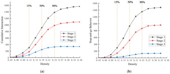
Figure 12.
Driving behavior statistics for the three stages. (a) Cumulative number of interactions; (b) cumulative number of stop-and-go behaviors.
Additionally, cumulative values for fuel consumption and traffic emissions (CO, HC, and NOx) are plotted across the different stages and density levels in Figure 13. The data show that fuel consumption and emissions exhibited a similar trend as density increased. For density, it was determined that the majority of vehicles in the roundabout operated within the density range of 0.12–0.24 (Figure 12 and Figure 13). At a density of around 0.12, a critical threshold for roundabout traffic efficiency and safety was observed. Effective speed exhibited a stable decline within the density range of 0.12–0.24, whereas after 0.24, it rapidly decreased. This indicates that the roundabout or specific local areas are approaching a bottleneck or gridlock. The focus of this study is precisely on reducing the frequency of such occurrences.
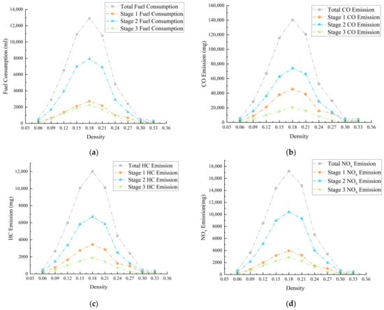
Figure 13.
Fuel consumption (a) and different traffic emissions (b–d) (for the density-based analysis, the statistically significant range was 0.06 and 0.33. Outside this range, the sample size was insufficient).
On the other hand, to more clearly illustrate the impact of stop-and-go behavior on fuel consumption and emissions, we calculated the average values for every ten seconds to represent the fuel consumption and emissions during that period, as shown in Figure 14. The results align with Tang et al.’s findings on traffic flow perturbations, where such disturbances significantly affected fuel consumption and emissions in the traffic system [60,65]. Specifically, stop-and-go behavior primarily occurred during the entrance stage, which is associated with higher fuel consumption and emissions, and the frequency of emission peaks remained consistent. Therefore, we concluded that
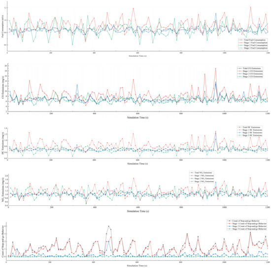
Figure 14.
Fuel consumption, emissions, and stop-and-go behavior statistics throughout the simulation.
- (1)
- The occurrences of interaction behavior and stop-and-go behavior are highly correlated.
- (2)
- The entrance stage is the most influential factor in roundabout traffic systems, where stop-and-go behavior predominantly occurs, leading to the highest average fuel consumption and emissions.
- (3)
- Seventy-five percent of these behaviors occur when the density ranges between 0.12 and 0.24.
Therefore, we propose the following assumptions and optimization strategies based on these observations: space-based strategies (strategy 1 and 2) and behavior-based strategies (strategy 3 and 4):
3.2.1. Implementing Dedicated Right-Turn Lanes (Strategy 1)
Due to the improper configuration of space for each lane entering the roundabout, the utilization rate of the outermost lane for right turns was very low. The low utilization of the outermost lane for right turns led most vehicles to interact within the inner three lanes. Therefore, we propose several methods:
- All vehicles aiming for the adjacent right road are prioritized to exit the roundabout in the outermost lane (R4).
- Vehicles traveling in R3 and aiming for R4 are allowed to change lanes outward at any time.
3.2.2. Road B Splitter Island Optimization (Strategy 2)
This strategy focus on a splitter island at Road B within the scope of this study. Due to changes in urban land use functions, the traffic flow at Road B, which originally had bidirectional access to the roundabout, now only has vehicles exiting the roundabout, as in the observation period. Additionally, the configuration of the splitter island does not align with the current traffic flow conditions, failing to effectively divert traffic and instead occupying traffic space within the roundabout that was originally meant for normal vehicle flow. Considering congestion and real-world conditions, we removed the splitter island (Red Area in Figure 1).
3.2.3. Threshold Control Strategy (Strategy 3)
To effectively control roundabout density and reduce fuel consumption and emissions, entry rules based on roundabout density were established:
- When the density exceeds 0.24, vehicle entry to the roundabout is restricted.
- When the density is between 0.18 and 0.24, the entry rate for each entrance is limited to 1.5 s per vehicle.
- When the density is below 0.18, vehicles enter the roundabout normally.
3.2.4. Path Selection Based on Density Recognition (Strategy 4)
Drivers will be prompted to make informed lane selection decisions before entering or navigating within the roundabout, thereby avoiding congestion and hazardous interactions. We optimized the decision-making algorithm in the original model, allowing drivers to choose the optimal path based on lane density when permitted by the algorithm. Based on the density in the density study zone (Figure 9), the probability of vehicles for the three lanes uses the following formula:
where is defined as the probability of choosing lane in the density study zone, represent the inner, typical, and outer lanes, respectively. is a calibration parameter that adjusts the vehicle’s sensitivity to lane density, with higher values giving more weight to lanes with lower density, in this study . is the attractiveness of the different ring lanes, defined by the max density and current density of the lane l. That is
where and are the current density and the maximum density (for ease of calculation, the maximum density is 0.24) of each lane, respectively. is calculated based on lane l (Equation (5)).
4. Result Analysis and Discussion
Here, we first analyzed the optimization effects of the different strategies on total fuel consumption and emissions. Subsequently, we evaluated the strategies based on the average values of fuel consumption and emissions, alongside their effects on improving the traffic efficiency at different stages.
4.1. Overall Results across Simulations
Here, we explored the impact of the various optimization strategies on the roundabout traffic flow from two perspectives: (1) overall fuel consumption and emissions; and (2) traffic efficiency.
4.1.1. Total Fuel Consumption and Emissions
We recorded the cumulative fuel consumption and emissions across different traffic densities for the four optimization strategies (Figure 15), while also calculating the optimization effectiveness at various stages under different densities (the reduction rates of fuel consumption and emissions) (Table A1, Table A2, Table A3 and Table A4). To further highlight the comparative optimization capabilities of the four strategies, we documented their emission reductions relative to the original model (Table 2). We observed an overall decrease in total fuel consumption and emissions for all four strategies, with peak emissions shifting towards lower density areas (0.09–0.15). Overall, the behavior-based optimization strategies outperformed the space-based ones, with Strategy 4 exhibiting the best optimization effects. Specifically, the total reductions in fuel consumption and traffic emissions (CO, HC, and NOx) were 9994.10 mL, 256,380.08 mg, 146,74.98 mg, and 21,935.50 mg, respectively.
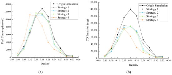
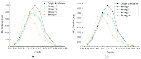
Figure 15.
Total fuel consumption (a) and emissions (b–d).
Table 2.
Total reduction in fuel consumption and emissions for the four strategies.
4.1.2. Traffic Efficiency
Here, we shift our focus to traffic efficiency. By plotting the fundamental diagram (Figure 16a) and a stop-and-go chart based on density (Figure 16b), we analyzed the impact of the four optimization strategies on improving the roundabout traffic flow. In Figure 16a, we can observe an interesting phenomenon: although the behavior-based optimization strategies demonstrated better overall performance in fuel consumption and emissions, they did not provide superior traffic speed. In contrast, the space-based optimization strategies exhibited significantly better traffic performance. Specifically, Strategy 1 exhibited the best optimization performance, increasing the global average speed by 10.26%. Although Strategy 4 did not provide the best traffic performance (increasing by 8.88%), it still achieved the greatest reduction in stop-and-go movements (Figure 16b). This outcome relates to its strategy of density-based driving behaviors that help avoid traffic congestion.
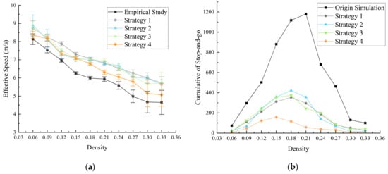
Figure 16.
Traffic flow characteristic indicators. (a) Fundamental diagram; (b) cumulative number of stop-and-go behavior.
Clearly, the different types of optimization strategies produced distinct effects on fuel consumption, emissions, and traffic efficiency. The behavior-based optimization strategies significantly reduced fuel consumption and emissions, improved the overall fluidity of roundabout traffic, and minimized the occurrence of stop-and-go behaviors. However, this came at the cost of spending more time within the roundabout, resulting in only modest increases in effective speed. In contrast, the space-based optimization strategies provided more interactive space, improving roundabout speed, though their impact on reducing congestion and emissions was limited.
4.2. Results Analysis in Different Stages
4.2.1. Results in the Entrance Stage
To further explore the underlying causes of the overall results, we focused on examining fuel consumption and emissions across the three stages, assessing the influence of the optimization strategies on vehicles in each stage. We analyzed the frequency of stop-and-go events produced by the four strategies across the different stages, observing that all strategies significantly reduced these occurrences compared to the original model, with the entrance stage exhibiting a notably higher frequency than the other stages (Table 3). Consequently, we calculated the reductions in fuel consumption and emissions for each strategy and plotted the trends of average emissions across varying densities (Figure 17). The results showed that Strategy 4 consistently delivered the most effective optimization, particularly in reducing emissions. Specifically, the reductions were 0.042 mL/s in fuel consumption, 0.839 mg/s for CO, 0.033 mg/s for HC, and 0.070 mg/s for NOx.
Table 3.
Number of stop-and-go behaviors for the four strategies.
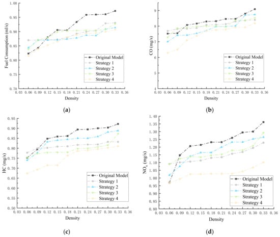
Figure 17.
Stage 1: fuel consumption (a) and different traffic emissions (b–d).
The optimization effects of these strategies were similar to the original model at low densities (0.06–0.12), with space-based optimization strategies performing relatively better. Under low traffic flow, most vehicles maintained free-flow movement, where additional space offered limited improvement. As the density increased, however, the advantage of space-based optimization diminished. In contrast, the behavior-based optimization strategies maximized the avoidance of stopping at entry points and reduced congestion, thereby decreasing fuel consumption and emissions. Specifically, Strategy 4, which achieved the best optimization results, enabling vehicles to pre-select lanes during the entrance stage. This not only avoided the potential congestion caused by human interference but also enhanced the utilization of available road space. In dynamic traffic systems, this approach can effectively increase interaction space, outperforming space-based optimization strategies. In particular, in the entrance stage, Strategy 1 achieved reductions of 8.25%, 32.64%, 18.48%, and 18.09% in fuel consumption and emissions, respectively—far below the performance of Strategy 4 (see Table 4 for details).
Table 4.
Stage 1 reduction in fuel consumption and emissions for the four strategies.
4.2.2. Results in the Following Stage and Exit Stage
To study the fuel consumption and emissions of vehicles traveling within the roundabout, we recorded and plotted the density-based average instantaneous emissions for the following stage and exit stage (Figure A1 and Figure A2). Overall, all four optimization strategies demonstrated a certain level of emission reductions, with their effects being almost identical. This was because these strategies primarily target traffic flow behavior and space optimization during the entry stage. Once fully integrated into the roundabout traffic flow, the effectiveness of the optimization strategies diminished.
In the following stage (stage 2), vehicle movement follows a multi-lane, unidirectional car-following model, where the fuel consumption and emissions are determined by the vehicle distribution and density across lanes, similarly to in the original model. However, Strategy 4, through pre-selection of lanes and density-based lane-changing decisions within the roundabout, enhanced the road utilization and reduced the frequency of stop-and-go occurrences. As a result, Strategy 4 also exhibited a certain degree of optimization capability in the following stage. In the exit stage (stage 3), benefiting from the optimization of interactions with incoming vehicles during the entrance stage, the exit area similarly gains a broader interaction range. As a result, fuel consumption and emissions were consistent with the original model at low densities. However, as the density increased, all optimization strategies exhibited comparable levels of optimization performance. In these two stages, Strategy 4’s congestion-avoidance approach reduced fuel consumption and emissions by 0.16 mL/s, 4.47 mg/s, 0.33 mg/s, and 1.30 mg/s in Stage 2, and 0.27 mL/s, 2.15 mg/s, 0.30 mg/s, and 0.70 mg/s in Stage 3.
All four optimization strategies were effective, with Strategy 4 achieving optimal fuel consumption and emissions, while Strategy 1 provided the highest traffic efficiency. For total fuel consumption and traffic emissions, Strategy 4 achieved reduction rates of 18.40%, 43.20%, 28.98%, and 30.02%, while Strategy 1 achieved reductions of 8.25%, 32.63%, 18.48%, and 18.09%, respectively.
In summary, at low densities, where the vehicle interaction frequency is low, strategies focused on spatial optimization offer limited improvements. As the density increases and interaction frequency rises, optimization strategies begin to impact traffic. Among these, strategies based on vehicle driving behavior achieve significant improvements. Nevertheless, they may still result in less than optimal traffic efficiency. Thus, optimizing fuel consumption and emissions in roundabout traffic flow requires considering multiple factors.
4.3. Discussion
Lakouari et al. [32] studied vehicle emissions at a single-lane roundabout using various injection and extraction rates. They found that traffic emissions are closely linked to vehicle speed.
However, in our study, a higher traffic speed did not necessarily indicate the optimal emissions efficiency. At lower densities, there is a certain synergistic relationship between speed and emissions. At medium to high densities, speed has less effect on emissions.
This difference arises because previous models simplified the roundabout to a single-lane, one-way configuration, representing density only through injection and extraction rates, without accounting for real-time variations in internal traffic density on vehicle emissions. Moreover, they calculated the vehicle emissions in only one road of the roundabout. However, we took into consideration various factors that could impact fuel consumption and emissions: vehicle trajectories, entry traffic space, vehicle entry decisions into the roundabout, traffic control, vehicle interaction behavior, and stop-and-go behavior, which provided a clearer understanding of traffic emission behaviors in relation to various traffic-related parameters.
The analysis of the simulation results revealed that it is very challenging to optimize traffic characteristics for all traffic states using a single strategy alone. The optimization of roundabout traffic flow must be adapted based on traffic-related parameters, particularly density and traffic flow decisions.
Overall, compared to strategies focusing on vehicle decisions and behavior optimization (Strategies 3 and 4), optimization strategies based on traffic space updates (Strategies 1 and 2) can effectively improve roundabout traffic flow efficiency, though they offer less favorable results in terms of fuel consumption and emissions. Most vehicular emissions are generated in the entrance stage (Stage 1), due to acceleration and deceleration from interaction behaviors.
The density at which vehicles operate also needs to be considered. At lower densities, space-based strategies (Strategies 1 and 2) offer the best reduction in emissions. As density increases, behavior-based strategies (Strategies 3 and 4) result in lower emissions. Nonetheless, both types of optimization strategies can reduce fuel consumption and emissions in roundabout traffic flow to a certain extent. Moreover, the study of vehicular traffic using autonomous vehicles has garnered significant attention from scholars, who view them as a promising solution to traffic-related issues. Zhao et al. [66] investigated the impact of autonomous vehicles on fuel consumption and traffic emissions in various traffic scenarios. They found that the advantages of connected and autonomous vehicles (CAVs) are most pronounced at signalized intersections, with fuel consumption and emissions potentially reduced by up to 32% when the penetration rate of CAVs reaches 100%. One of the advantages of this study is that it allows for the incorporation of autonomous vehicles into the proposed model, enabling an investigation of their impact on roundabout traffic flow characteristics.
5. Conclusions
As the depletion of non-renewable resources intensifies, the pursuit of sustainable development goals has emerged as a global priority. However, intricate traffic flows, exemplified by roundabouts, are often associated with elevated emissions and increased fuel consumption. To tackle this challenge, this study developed a sophisticated traffic flow model grounded in cellular automata, aimed at simulating the traffic dynamics that influence fuel consumption and emissions on large roundabouts. The model incorporates a vehicle movement framework (the NaSch model), a three-stage vehicle decision-making model, and a motor vehicle fuel consumption and emissions model (the VT-Micro model). Numerical validation confirmed the model’s efficacy in accurately replicating complex traffic behaviors within large roundabouts. The findings revealed a significant correlation between fuel consumption and emissions, particularly in relation to the entrance stage and the frequency of stop-and-go events occurring within the roundabout.
Building on these insights, we proposed four optimization strategies that focused on both spatial and behavioral factors, all of which effectively mitigated fuel consumption and emissions, while enhancing the overall efficiency of roundabout traffic. Furthermore, our analysis indicated that improved traffic efficiency does not inherently lead to reductions in fuel consumption and emissions. This underscores the importance of employing a synergistic approach that combines multiple optimization strategies to optimize urban traffic efficiency.
This paper aimed to address the following limitations and gaps in previous research, while also discovering several novel insights achieved during the study:
- This study addressed the lack of research on the impact of specific micro-level vehicle behaviors on fuel consumption and emissions in roundabout studies.
- This study developed a multi-lane roundabout model that included a large six-way intersection, effectively replicating the complex traffic behaviors within it.
- This study identified traffic factors that influence fuel consumption and emissions in roundabout traffic, such as the flow of traffic during the entrance stage and the frequency of stop-and-go events.
- The strategies proposed in this study effectively optimized roundabout traffic efficiency and reduced fuel consumption and emissions, achieving reductions of up to 18.40%, 43.20%, 28.98%, and 30.02%, along with a 10.26% increase in traffic efficiency.
In addition, based on the fuel consumption, emissions, and traffic characteristic indicators derived from the complex traffic flow model, we observed that, for roundabouts as complex systems, the entrance stage holds greater significance than other stages. On the one hand, optimizing the traffic flow in the entrance stage enhances downstream traffic efficiency and reduces emissions; on the other, promptly processing incoming traffic benefits vehicles exiting the roundabout. Additionally, as highlighted by the contrasting results for efficiency and emissions between Strategies 1 and 4, in traffic flow optimization research, it is crucial to address the inherent trade-offs between overall system efficiency and emission reduction. These findings provide valuable insights into how various traffic-related parameters influence vehicle emissions. By enhancing our understanding of these relationships, we can refine optimization strategies to reduce emissions and enhance traffic efficiency. This knowledge can contribute to the academic discourse on sustainable urban traffic management and can offer practical insights for policymakers and traffic engineers implementing effective measures in roundabouts and similar systems. Ultimately, applying these insights can foster environmentally friendly transportation solutions and advance broader sustainable development goals.
Author Contributions
Conceptualization, H.S. and X.L.; methodology, X.L.; software, G.W.; validation, X.L., Y.G. and G.W.; formal analysis, H.S.; investigation, Y.G.; resources, H.S. and S.Z.; data curation, X.L.; writing—original draft preparation, X.L.; writing—review and editing, X.L.; visualization, X.L. and S.Z.; supervision, H.S. and S.Z.; project administration, Y.G.; funding acquisition, H.S. and S.Z. All authors have read and agreed to the published version of the manuscript.
Funding
This research was funded by The 15th Graduate Education Innovation Fund of Wuhan Institute of Technology, grant number CX2023351; the 2023 Hubei Provincial Science and Technology Plan Project, grant number 2023006; the 2023 Hubei Provincial Social Science Fund, grant number 2023221.
Data Availability Statement
Data available on request due to privacy restrictions.
Acknowledgments
We appreciate the participation and tremendous support from all informants.
Conflicts of Interest
The authors declare no conflicts of interest.
Appendix A
Table A1.
Fuel consumption reduction rates (%) for different optimization strategies (S1–S4) at various densities and stages.
Table A1.
Fuel consumption reduction rates (%) for different optimization strategies (S1–S4) at various densities and stages.
| Stage 1 | Stage 2 | Stage 3 | ||||||||||
|---|---|---|---|---|---|---|---|---|---|---|---|---|
| Density | S 1 (%) | S 2 (%) | S 3 (%) | S 4 (%) | S 1 (%) | S 2 (%) | S 3 (%) | S 4 (%) | S 1 (%) | S 2 (%) | S 3 (%) | S 4 (%) |
| 0.06 | 20.59 | −5.13 | 14.43 | −49.50 | 40.40 | −10.11 | −6.46 | −50.94 | 50.50 | 2.05 | 5.88 | −79.08 |
| 0.09 | 34.37 | 33.89 | 13.07 | −35.21 | 37.80 | 32.36 | 6.80 | −11.94 | 21.94 | 30.04 | −6.80 | −55.06 |
| 0.12 | −9.49 | −33.14 | −13.24 | −48.56 | −6.06 | −22.85 | −13.13 | −21.04 | −21.73 | −56.34 | −29.27 | −71.03 |
| 0.15 | −17.85 | 3.98 | 10.03 | −47.67 | −15.50 | −12.26 | −7.90 | −24.16 | −9.33 | −13.22 | −1.09 | −25.58 |
| 0.18 | 2.85 | 14.74 | 11.31 | 15.98 | 3.44 | 2.90 | 9.27 | 31.57 | 10.08 | 6.03 | 16.04 | 22.65 |
| 0.21 | 15.54 | 20.87 | 32.57 | 54.86 | 17.88 | 15.23 | 23.24 | 57.40 | 12.99 | 21.01 | 16.06 | 54.73 |
| 0.24 | 9.91 | 39.63 | 20.95 | 57.37 | 8.36 | 38.41 | 24.84 | 60.06 | 10.55 | 47.71 | 16.98 | 56.38 |
| 0.27 | 12.91 | 52.11 | 27.85 | 71.79 | 27.68 | 62.70 | 59.30 | 70.59 | 26.48 | 66.92 | 50.49 | 76.18 |
| 0.3 | −25.61 | 13.84 | −81.78 | 60.04 | −15.07 | 34.93 | 23.53 | 34.95 | −31.93 | 53.35 | 6.51 | 35.44 |
| 0.33 | 26.37 | 58.74 | 10.58 | 73.45 | 54.03 | 57.53 | 56.91 | 79.51 | 29.59 | 58.90 | 28.03 | 82.90 |
Table A2.
CO emissions reduction rates (%) for different optimization strategies (S1–S4) at various densities and stages.
Table A2.
CO emissions reduction rates (%) for different optimization strategies (S1–S4) at various densities and stages.
| Stage 1 | Stage 2 | Stage 3 | ||||||||||
|---|---|---|---|---|---|---|---|---|---|---|---|---|
| Density | S 1 (%) | S 2 (%) | S 3 (%) | S 4 (%) | S 1 (%) | S 2 (%) | S 3 (%) | S 4 (%) | S 1 (%) | S 2 (%) | S 3 (%) | S 4 (%) |
| 0.06 | 53.27 | 39.06 | 49.33 | 13.02 | 20.20 | −4.94 | −6.65 | −39.45 | 29.08 | 5.98 | 6.51 | −77.90 |
| 0.09 | 57.81 | 65.87 | 51.36 | 35.79 | 37.56 | 41.87 | 21.33 | 11.73 | 37.26 | 41.03 | 8.78 | −30.42 |
| 0.12 | 29.29 | 24.10 | 35.26 | 22.76 | −10.18 | −7.19 | 2.22 | −1.82 | −43.76 | −43.64 | −19.69 | −63.37 |
| 0.15 | 52.77 | 44.72 | 47.70 | 26.08 | 14.99 | 8.32 | 9.21 | 3.47 | 21.21 | 6.61 | 13.24 | −4.01 |
| 0.18 | 45.39 | 48.30 | 47.43 | 50.98 | 12.37 | 16.44 | 22.69 | 45.00 | 18.74 | 19.06 | 27.09 | 31.10 |
| 0.21 | 67.75 | 57.51 | 65.74 | 79.41 | 41.67 | 29.12 | 37.43 | 67.96 | 39.07 | 37.77 | 33.84 | 63.87 |
| 0.24 | 64.29 | 71.04 | 59.87 | 77.74 | 46.68 | 55.08 | 42.89 | 72.15 | 45.97 | 58.08 | 32.53 | 62.74 |
| 0.27 | 47.54 | 75.96 | 64.82 | 86.24 | 50.12 | 71.17 | 66.32 | 79.08 | 33.55 | 73.96 | 63.14 | 82.82 |
| 0.3 | 38.83 | 54.30 | −1.53 | 76.55 | 31.54 | 53.74 | 43.48 | 45.41 | 8.30 | 62.49 | 23.19 | 42.77 |
| 0.33 | 61.50 | 75.94 | 46.28 | 85.23 | 77.24 | 57.63 | 60.91 | 85.06 | 68.83 | 69.26 | 47.85 | 86.19 |
Table A3.
HC emissions reduction rates (%) for different optimization strategies (S1–S4) at various densities and stages.
Table A3.
HC emissions reduction rates (%) for different optimization strategies (S1–S4) at various densities and stages.
| Stage 1 | Stage 2 | Stage 3 | ||||||||||
|---|---|---|---|---|---|---|---|---|---|---|---|---|
| Density | S 1 (%) | S 2 (%) | S 3 (%) | S 4 (%) | S 1 (%) | S 2 (%) | S 3 (%) | S 4 (%) | S 1 (%) | S 2 (%) | S 3 (%) | S 4 (%) |
| 0.06 | 29.50 | 20.19 | 36.03 | −13.34 | −11.97 | −7.35 | −5.44 | −46.09 | −25.74 | 2.45 | 7.43 | −76.06 |
| 0.09 | 23.31 | 51.94 | 35.71 | 8.06 | 2.62 | 34.48 | 10.49 | −8.11 | 0.17 | 35.32 | 1.26 | −44.73 |
| 0.12 | 20.13 | 3.16 | 17.53 | −0.48 | 7.43 | −18.72 | −10.89 | −16.05 | −17.47 | −56.43 | −29.71 | −69.56 |
| 0.15 | 34.26 | 30.60 | 35.36 | 2.56 | −8.70 | −7.85 | −4.14 | −18.59 | 4.84 | −9.21 | 2.97 | −21.25 |
| 0.18 | 43.36 | 35.62 | 34.83 | 39.79 | 14.80 | 6.37 | 13.20 | 34.92 | 17.12 | 9.29 | 18.79 | 24.62 |
| 0.21 | 55.19 | 44.85 | 54.76 | 71.12 | 29.16 | 17.85 | 26.12 | 59.39 | 34.27 | 24.49 | 20.27 | 57.14 |
| 0.24 | 45.79 | 58.66 | 44.46 | 71.57 | 19.11 | 41.76 | 29.21 | 62.94 | 11.92 | 50.25 | 21.06 | 58.95 |
| 0.27 | 62.62 | 66.60 | 50.61 | 81.65 | 43.48 | 64.36 | 60.55 | 72.12 | 43.53 | 68.60 | 52.92 | 76.79 |
| 0.3 | −66.90 | 32.52 | −45.91 | 70.95 | −79.76 | 36.69 | 24.75 | 33.20 | −79.08 | 54.62 | 9.12 | 34.75 |
| 0.33 | 66.05 | 69.08 | 35.59 | 82.33 | 50.36 | 56.45 | 58.12 | 80.93 | 25.42 | 60.01 | 30.54 | 83.52 |
Table A4.
NOx emissions reduction rates (%) for different optimization strategies (S1–S4) at various densities and stages.
Table A4.
NOx emissions reduction rates (%) for different optimization strategies (S1–S4) at various densities and stages.
| Stage 1 | Stage 2 | Stage 3 | ||||||||||
|---|---|---|---|---|---|---|---|---|---|---|---|---|
| Density | S 1 (%) | S 2 (%) | S 3 (%) | S 4 (%) | S 1 (%) | S 2 (%) | S 3 (%) | S 4 (%) | S 1 (%) | S 2 (%) | S 3 (%) | S 4 (%) |
| 0.06 | 23.01 | 8.52 | 20.69 | −22.74 | −9.30 | −6.11 | −3.88 | −43.65 | −16.39 | 8.98 | 10.11 | −78.67 |
| 0.09 | 11.08 | 44.47 | 20.53 | −9.94 | 8.21 | 38.76 | 14.06 | 3.91 | −1.36 | 33.79 | −3.72 | −47.43 |
| 0.12 | 3.16 | −17.30 | −0.54 | −21.92 | 13.28 | −13.94 | −2.42 | −9.44 | −10.25 | −42.89 | −17.78 | −61.22 |
| 0.15 | 17.86 | 12.85 | 14.84 | −22.93 | −0.87 | −2.27 | 1.03 | −8.98 | 10.74 | 0.13 | 7.83 | −10.99 |
| 0.18 | 29.13 | 23.25 | 17.61 | 26.06 | 19.78 | 12.40 | 18.19 | 40.39 | 21.17 | 13.82 | 23.17 | 28.56 |
| 0.21 | 42.89 | 29.05 | 41.20 | 63.65 | 34.74 | 24.78 | 33.09 | 64.52 | 39.11 | 31.21 | 26.24 | 59.66 |
| 0.24 | 31.83 | 47.58 | 29.61 | 61.49 | 26.88 | 49.74 | 36.38 | 68.08 | 14.58 | 53.41 | 25.23 | 58.22 |
| 0.27 | 50.82 | 60.09 | 39.94 | 75.85 | 49.61 | 68.38 | 63.50 | 76.92 | 50.16 | 70.02 | 57.69 | 80.42 |
| 0.3 | −66.57 | 41.95 | −26.02 | 70.99 | −33.14 | 51.67 | 40.76 | 52.63 | −48.10 | 60.36 | 19.10 | 41.06 |
| 0.33 | 61.03 | 64.69 | 10.80 | 75.42 | 53.86 | 63.21 | 60.55 | 83.89 | 35.17 | 63.67 | 35.21 | 82.60 |
Appendix B
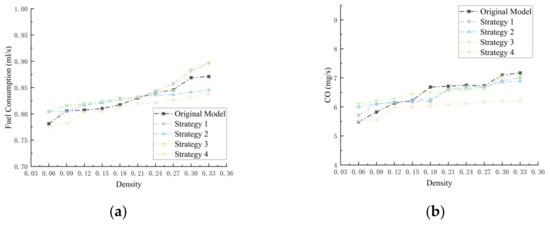
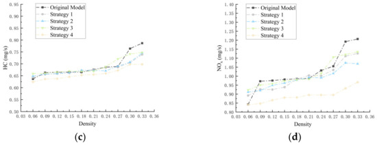
Figure A1.
Stage 2: fuel consumption (a) and different traffic emissions (b–d).
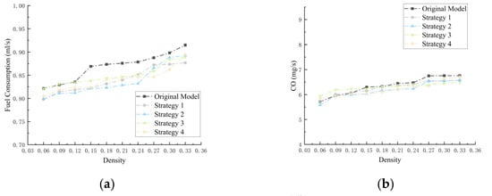
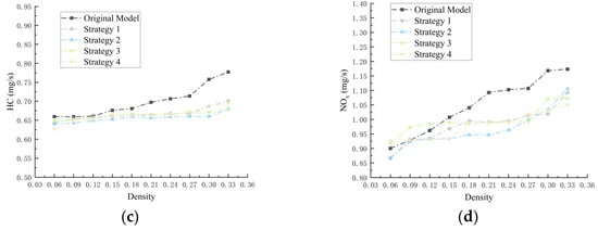
Figure A2.
Stage 3: fuel consumption (a) and different traffic emissions (b–d).
References
- Kumar, P.G.; Lekhana, P.; Tejaswi, M.; Chandrakala, S. Effects of vehicular emissions on the urban environment-a state of the art. Mater. Today Proc. 2021, 45, 6314–6320. [Google Scholar] [CrossRef]
- Ministry of Environmental Protection. Beijing Releases Latest PM2.5 Source Analysis: Three-Quarters of Local Pollutants Come from Vehicles. Available online: https://www.gov.cn/xinwen/2014-04/16/content_2660844.htm (accessed on 5 August 2024).
- Gouveia, N.; Rodriguez-Hernandez, J.L.; Kephart, J.L.; Ortigoza, A.; Betancourt, R.M.; Sangrador, J.L.T.; Rodriguez, D.A.; Roux, A.V.; Sanchez, B.; Yamada, G. Short-term associations between fine particulate air pollution and cardiovascular and respiratory mortality in 337 cities in Latin America. Sci. Total Environ. 2024, 920, 171073. [Google Scholar] [CrossRef] [PubMed]
- Macioszek, E.; Kurek, A. Roundabout users subjective safety—Case study from upper silesian and masovian voivodeships (Poland). Trans. Transp. Sci. 2020, 11, 39–50. [Google Scholar] [CrossRef]
- Macioszek, E. Roundabouts as aesthetic road solutions for organizing landscapes. Zesz. Nauk. Transp./Politech. Śląska 2022, 115, 53–62. [Google Scholar] [CrossRef]
- Madziel, M.; Campisi, T. Assessment of vehicle emissions at roundabouts: A comparative study of PEMS data and microscale emission model. Arch. Transp. 2022, 63, 35–51. [Google Scholar] [CrossRef]
- Meneguzzer, C.; Gastaldi, M.; Rossi, R.; Gecchele, G.; Prati, M.V. Comparison of exhaust emissions at intersections under traffic signal versus roundabout control using an instrumented vehicle. Transp. Res. Procedia 2017, 25, 1597–1609. [Google Scholar] [CrossRef]
- Meneguzzer, C.; Gastaldi, M.; Arboretti Giancristofaro, R. Before-and-After Field Investigation of the Effects on Pollutant Emissions of Replacing a Signal-Controlled Road Intersection with a Roundabout. J. Adv. Transp. 2018, 2018, 3940362. [Google Scholar] [CrossRef]
- Hallmark, S.L.; Wang, B.; Mudgal, A.; Isebrands, H. On-road evaluation of emission impacts of roundabouts. Transp. Res. Rec. 2011, 2265, 226–233. [Google Scholar] [CrossRef]
- Rosero, F.; Fonseca, N.; López, J.M.; Casanova, J. Effects of passenger load, road grade, and congestion level on real-world fuel consumption and emissions from compressed natural gas and diesel urban buses. Appl. Energy 2021, 282, 116195. [Google Scholar] [CrossRef]
- Krause, J.; Thiel, C.; Tsokolis, D.; Samaras, Z.; Rota, C.; Ward, A.; Prenninger, P.; Coosemans, T.; Neugebauer, S.; Verhoeve, W. EU road vehicle energy consumption and CO2 emissions by 2050–Expert-based scenarios. Energy Policy 2020, 138, 111224. [Google Scholar] [CrossRef]
- Wang, Q.; Xue, M.; Lin, B.L.; Lei, Z.F.; Zhang, Z.Y. Well-to-wheel analysis of energy consumption, greenhouse gas and air pollutants emissions of hydrogen fuel cell vehicle in China. J. Clean. Prod. 2020, 275, 123061. [Google Scholar] [CrossRef]
- Xue, H.; Jiang, S.; Liang, B. A study on the model of traffic flow and vehicle exhaust emission. Math. Probl. Eng. 2013, 2013, 736285. [Google Scholar] [CrossRef]
- Coelho, M.C.; Farias, T.L.; Rouphail, N.M. A methodology for modelling and measuring traffic and emission performance of speed control traffic signals. Atmos. Environ. 2005, 39, 2367–2376. [Google Scholar] [CrossRef]
- Zegeye, S.K.; De Schutter, B.; Hellendoorn, J.; Breunesse, E.A.; Hegyi, A. Integrated macroscopic traffic flow, emission, and fuel consumption model for control purposes. Transp. Res. Part C Emerg. Technol. 2013, 31, 158–171. [Google Scholar] [CrossRef]
- Anderson, P.W. More Is Different: Broken symmetry and the nature of the hierarchical structure of science. Science 1972, 177, 393–396. [Google Scholar] [CrossRef]
- Africa, D.D.; Dy Quiangco, R.B.; Go, C.K. Lag and duration of leader–follower relationships in mixed traffic using causal inference. Chaos Interdiscip. J. Nonlinear Sci. 2024, 34, 013130. [Google Scholar] [CrossRef]
- Gao, R.; Wang, W.; Xiong, X.; Li, J.J.; Xu, C. Effect of curing temperature on the mechanical properties and pore structure of cemented backfill materials with waste rock-tailings. Constr. Build. Mater. 2023, 409, 133850. [Google Scholar] [CrossRef]
- Gao, R.; Wang, W.; Zhou, K.; Zhao, Y.L.; Yang, C.; Ren, Q.F. Optimization of a Multiphase Mixed Flow Field in Backfill Slurry Preparation Based on Multiphase Flow Interaction. ACS Omega 2023, 8, 34698–34709. [Google Scholar] [CrossRef]
- Zhang, B.; Shang, L.; Chen, D. A study on the traffic intersection vehicle emission base on urban microscopic traffic simulation model. In Proceedings of the 2009 First International Workshop on Education Technology and Computer Science, Wuhan, China, 7–8 March 2009; IEEE: Piscataway, NJ, USA, 2009; Volume 2, pp. 789–794. [Google Scholar]
- Beza, A.D.; Maghrour Zefreh, M.; Torok, A. Impacts of different types of automated vehicles on traffic flow characteristics and emissions: A microscopic traffic simulation of different freeway segments. Energies 2022, 15, 6669. [Google Scholar] [CrossRef]
- Makridis, M.; Mattas, K.; Mogno, C.; Ciuffo, B.; Fontaras, G. The impact of automation and connectivity on traffic flow and CO2 emissions. A detailed microsimulation study. Atmos. Environ. 2020, 226, 117399. [Google Scholar] [CrossRef]
- Macioszek, E. Analysis of driver behaviour at roundabouts in Tokyo and the Tokyo surroundings. In Modern Traffic Engineering in the System Approach to the Development of Traffic Networks, Proceedings of the 16th Scientific and Technical Conference, “Transport Systems. Theory and Practice 2019”, Katowice, Poland, 16–18 September 2019; Selected Papers 16; Springer International Publishing: Cham, Switzerland, 2020; pp. 216–227. [Google Scholar]
- Ahmed, A.; Rizvi SF, A.; Ahmad, F. Modelling Merging Behaviour of Drivers in Heterogeneous Traffic at Roundabouts. Eur. Transp. Trasp. Eur. 2024. [Google Scholar] [CrossRef]
- Rossi, R.; Meneguzzer, C.; Orsini, F.; Gastaldi, M. Gap-acceptance behavior at roundabouts: Validation of a driving simulator environment using field observations. Transp. Res. Procedia 2020, 47, 27–34. [Google Scholar] [CrossRef]
- Silvano, A.P.; Ma, X.; Koutsopoulos, H.N. When do drivers yield to cyclists at unsignalized roundabouts? Empirical evidence and behavioral analysis. Transp. Res. Rec. 2015, 2520, 25–31. [Google Scholar] [CrossRef]
- Li, C.; Liu, S.; Xu, G.; Cen, X. Influence of driver’s yielding behavior on pedestrian-vehicle conflicts at a two-lane roundabout using fuzzy cellular automata. J. Cent. South Univ. 2022, 29, 346–358. [Google Scholar] [CrossRef]
- Patnaik, A.K.; Rao, S.; Krishna, Y.; Bhuyan, P.K. Empirical capacity model for roundabouts under heterogeneous traffic flow conditions. Transp. Lett. 2017, 9, 152–165. [Google Scholar] [CrossRef]
- Yoshioka, K.; Hnakamura, H.; Shimokawa, S.; Morita, H. An analysis on impact of roundabout geometric elements on driving behavior. J. East. Asia Soc. Transp. Stud. 2017, 12, 1783–1796. [Google Scholar]
- Guerrieri, M.; Mauro, R.; Parla, G.; Tollazzi, T. Analysis of kinematic parameters and driver behavior at turbo roundabouts. J. Transp. Eng. Part A Syst. 2018, 144, 04018020. [Google Scholar] [CrossRef]
- Fernandes, P.; Pereira, S.R.; Bandeira, J.M.; Vasconcelos, L.; Silva, A.B.; Coelho, M.C.; Driving around turbo-roundabouts, vs. conventional roundabouts: Are there advantages regarding pollutant emissions? Int. J. Sustain. Transp. 2016, 10, 847–860. [Google Scholar] [CrossRef]
- Lakouari, N.; Oubram, O.; Bassam, A.; Hernandez, S.E.P.; Marzoug, R.; Ez-Zahraouy, H. Modeling and simulation of CO2 emissions in roundabout intersection. J. Comput. Sci. 2020, 40, 101072. [Google Scholar] [CrossRef]
- Bahmankhah, B.; Macedo, E.; Fernandes, P.; Coelho, M. Micro driving behaviour in different roundabout layouts: Pollutant emissions, vehicular jerk, and traffic conflicts analysis. Transp. Res. Procedia 2022, 62, 501–508. [Google Scholar] [CrossRef]
- Fernandes, P.; Tomás, R.; Acuto, F.; Pascale, A.; Bahmankhah, B.; Guarnaccia, C.; Granà, A.; Coelho, M. Impacts of roundabouts in suburban areas on congestion-specific vehicle speed profiles, pollutant and noise emissions: An empirical analysis. Sustain. Cities Soc. 2020, 62, 102386. [Google Scholar] [CrossRef]
- Wang, H.; Wen, H.; You, F.; Xu, J.; Kui, H. Motor vehicle emission modeling and software simulation computing for roundabout in urban city. Math. Probl. Eng. 2013, 2013, 312396. [Google Scholar] [CrossRef]
- Małecki, K.; Wątróbski, J. Cellular automaton to study the impact of changes in traffic rules in a roundabout: A preliminary approach. Appl. Sci. 2017, 7, 742. [Google Scholar] [CrossRef]
- Hua, W.; Yue, Y.; Wei, Z.; Chen, J.; Wang, W. A cellular automata traffic flow model with spatial variation in the cell width. Phys. A Stat. Mech. Its Appl. 2020, 556, 124777. [Google Scholar] [CrossRef]
- Zhu, L.; Tang, Y.; Yang, D. Cellular automata-based modeling and simulation of the mixed traffic flow of vehicle platoon and normal vehicles. Phys. A Stat. Mech. Its Appl. 2021, 584, 126368. [Google Scholar] [CrossRef]
- Liu, K.; Feng, T. Heterogeneous traffic flow cellular automata model mixed with intelligent controlled vehicles. Phys. A Stat. Mech. Its Appl. 2023, 632, 129316. [Google Scholar] [CrossRef]
- Zhao, H.T.; Zhao, X.; Lu, J.C.; Xin, L.Y. Cellular automata model for Urban Road traffic flow Considering Internet of Vehicles and emergency vehicles. J. Comput. Sci. 2020, 47, 101221. [Google Scholar] [CrossRef]
- Feng, T.; Liu, K.; Liang, C. An improved cellular automata traffic flow model considering driving styles. Sustainability 2023, 15, 952. [Google Scholar] [CrossRef]
- Jiang, C.; Li, R.; Chen, T.; Xu, C.H.; Li, L.; Li, S.F. A two-lane mixed traffic flow model with drivers’ intention to change lane based on cellular automata. Int. J. Bio-Inspired Comput. 2020, 16, 229–240. [Google Scholar] [CrossRef]
- Shang, X.C.; Li, X.G.; Xie, D.F.; Jia, B.; Jiang, R.; Liu, F. A data-driven two-lane traffic flow model based on cellular automata. Phys. A Stat. Mech. Its Appl. 2022, 588, 126531. [Google Scholar] [CrossRef]
- Qiang, X.H.; Huang, L. Traffic flow modeling in fog with cellular automata model. Mod. Phys. Lett. B 2021, 35, 2150180. [Google Scholar] [CrossRef]
- Wang, X.; Xue, Y.; Cen, B.; Zhang, P.; He, H.D. Study on pollutant emissions of mixed traffic flow in cellular automaton. Phys. A Stat. Mech. Its Appl. 2020, 537, 122686. [Google Scholar] [CrossRef]
- Liu, X.; Li, M.; Zeng, N.; Li, T. Investigation on Nonlinear Flow Behavior through Rock Rough Fractures Based on Experiments and Proposed 3-Dimensional Numerical Simulation. Geofluids 2020, 2020, 8818749. [Google Scholar] [CrossRef]
- Gao, R.; Zhou, K.; Zhou, Y.; Yang, C. Research on the fluid characteristics of cemented backfill pipeline transportation of mineral processing tailings. Alex. Eng. J. 2020, 59, 4409–4426. [Google Scholar] [CrossRef]
- Marzoug, R.; Lakouari, N.; Pérez Cruz, J.R.; Vega Gómez, C.J. Cellular Automata Model for Analysis and Optimization of Traffic Emission at Signalized Intersection. Sustainability 2022, 14, 14048. [Google Scholar] [CrossRef]
- Qiao, Y.; Xue, Y.; Wang, X.; Cen, B.L.; Wang, Y.; Pan, W.; Zhang, Y.X. Investigation of PM emissions in cellular automata model with slow-to-start effect. Phys. A Stat. Mech. Its Appl. 2021, 574, 125996. [Google Scholar] [CrossRef]
- Tian, J.; Zhu, C.; Jiang, R.; Treiber, M. Review of the cellular automata models for reproducing synchronized traffic flow. Transp. A Transp. Sci. 2021, 17, 766–800. [Google Scholar] [CrossRef]
- Ez-zahar, A.; Lakouari, N.; Oubram, O.; Velásquez Aguilar, J.G.; Ez-zahraouy, H. Simulation Analysis of Traffic Management in Roundabout Systems. In Proceedings of the2024 4th International Conference on Innovative Research in Applied Science, Engineering and Technology (IRASET), Fez, Morocco, 16–17 May 2024; IEEE: Piscataway, NJ, USA, 2024; pp. 1–7. [Google Scholar]
- Nagel, K.; Schreckenberg, M. A cellular automaton model for freeway traffic. J. Phys. I 1992, 2, 2221–2229. [Google Scholar] [CrossRef]
- de Gier, J.; Schadschneider, A.; Schmidt, J. Kardar-parisi-zhang universality of the nagel-schreckenberg model. Phys. Rev. E 2019, 100, 052111. [Google Scholar] [CrossRef]
- Ahn, K. Microscopic Fuel Consumption and Emission Modeling. Ph.D. Thesis, Virginia Tech, Blacksburg, VA, USA, 1998. [Google Scholar]
- Ahn, K.; Rakha, H.; Trani, A.; ASCE, M.; Aerde, M.V. Estimating vehicle fuel consumption and emissions based on instantaneous speed and acceleration levels. J. Transp. Eng. 2002, 128, 182–190. [Google Scholar] [CrossRef]
- Akcelik, R. Efficiency and drag in the power-based model of fuel consumption. Transp. Res. Part B Methodol. 1989, 23, 376–385. [Google Scholar] [CrossRef]
- Hooker, J.N. Optimal driving for single-vehicle fuel economy. Transp. Res. Part A Gen. 1988, 22, 183–201. [Google Scholar] [CrossRef]
- Rakha, H.; Ahn, K. Closure to “estimating vehicle fuel consumption and emissions based on instantaneous speed and acceleration levels” by kyoung Ahn, hesham rakha, antonio trani, and michel van aerde. J. Transp. Eng. 2003, 129, 579–581. [Google Scholar] [CrossRef]
- Wuhan’s New Energy Passenger Vehicle Market in 2023. Available online: https://mp.weixin.qq.com/s?__biz=MzAxNTE1OTM4OQ==&mid=2650660447&idx=1&sn=66f1cd0ee8573273e7dcc4e3d7c57941&chksm=8381276db4f6ae7bfe596ff977425d8f3dd7130545091b62cb360e3808dceebd6f25694f1128&scene=27 (accessed on 21 October 2024).
- Tang, T.Q.; Huang, H.J.; Shang, H.Y. Influences of the driver’s bounded rationality on micro driving behavior, fuel consumption and emissions. Transp. Res. Part D Transp. Environ. 2015, 41, 423–432. [Google Scholar] [CrossRef]
- Oh, C.; Choi, J.; Jung, S. Proactive vehicle emissions quantification from crash potential under stop-and-go traffic conditions. Transp. Policy 2016, 49, 86–92. [Google Scholar] [CrossRef]
- Wang, P.; Ma, Y.; Yu, H.; Wang, L.; Zhang, W. An Improved Stop and Go Model Considering Exhaust Emissions for Connected Vehicles. In Proceedings of the 2018 IEEE 7th Data Driven Control and Learning Systems Conference (DDCLS), Enshi, China, 25–27 May 2018; IEEE: Piscataway, NJ, USA, 2018; pp. 887–892. [Google Scholar]
- Karrouchi, M.; Rhiat, M.; Nasri, I.; Atmane, I.; Hirech, K.; Messaoudi, A.; Melhaoui, M. Practical investigation and evaluation of the Start/Stop system’s impact on the engine’s fuel use, noise output, and pollutant emissions. e-Prime-Adv. Electr. Eng. Electron. Energy 2023, 6, 100310. [Google Scholar] [CrossRef]
- Coelho, M.C.; Farias, T.L.; Rouphail, N.M. Effect of roundabout operations on pollutant emissions. Transp. Res. Part D Transp. Environ. 2006, 11, 333–343. [Google Scholar] [CrossRef]
- Li, X.; Cui, J.; An, S.; Parsafard, M. Stop-and-go traffic analysis: Theoretical properties, environmental impacts and oscillation mitigation. Transp. Res. Part B Methodol. 2014, 70, 319–339. [Google Scholar] [CrossRef]
- Zhao, B.; Lin, Y.; Hao, H.; Yao, Z.H. Fuel consumption and traffic emissions evaluation of mixed traffic flow with connected automated vehicles at multiple traffic scenarios. J. Adv. Transp. 2022, 2022, 6345404. [Google Scholar] [CrossRef]
Disclaimer/Publisher’s Note: The statements, opinions and data contained in all publications are solely those of the individual author(s) and contributor(s) and not of MDPI and/or the editor(s). MDPI and/or the editor(s) disclaim responsibility for any injury to people or property resulting from any ideas, methods, instructions or products referred to in the content. |
© 2024 by the authors. Licensee MDPI, Basel, Switzerland. This article is an open access article distributed under the terms and conditions of the Creative Commons Attribution (CC BY) license (https://creativecommons.org/licenses/by/4.0/).