Abstract
In this study, a grid-based precipitation quantile was estimated using long-term reanalysis precipitation data, considering the homogeneity of the annual maximum series (AMS) for the Korean Peninsula. For regions where significant changes in homogeneity were observed, the precipitation quantile was estimated using only the AMS from after the change point, and these results were compared with those from the original AMS. The examination of homogeneity revealed a significant increasing trend in homogeneity variability in the southeastern region of Korea. This change was particularly pronounced in the location parameter of the Gumbel distribution, resulting in an improved model fit. The change in precipitation quantile was most noticeable for a 2-year return period with a 36 h duration, with an average increase of approximately 11.5%. The results obtained from this study are anticipated to offer crucial foundational data for the design of hydraulic structures in regions with insufficient long-term ground observation data.
1. Introduction
Hydraulic structures are typically designed in accordance with the design flood corresponding to a specific return period. In theory, the most appropriate method for estimating this design flood is to perform frequency analysis using observed flood data. However, due to limitations such as insufficient observed discharge data and concerns about data reliability, direct statistical analysis using discharge data presents many challenges. Furthermore, the point where a new hydraulic structure is planned is likely to have no records of discharge, so the same problem occurs. To address these challenges, the frequency analysis method using precipitation data is being proposed to estimate precipitation quantiles, followed by a rainfall-runoff model to derive the design flood [1,2,3,4]. Therefore, the primary approach to estimate the design flood, which continues to be used to this day worldwide, involves performing frequency analysis on precipitation data, which are relatively easier to obtain, to estimate the precipitation quantile [5].
For this reason, obtaining an accurate precipitation quantile for the design return period is ultimately important in terms of estimating the design flood. Generally, frequency analysis techniques for precipitation are categorized into at-site frequency analysis and regional frequency analysis. The precipitation quantile is estimated using only the data from a given site in an at-site frequency analysis. In contrast, regional frequency analysis estimates the precipitation quantile by including not only the data from the target site but also from surrounding sites that are judged to be hydrologically homogeneous [6]. In other words, regional frequency analysis is a method that spatially compensates for the temporal limitations of the data from the target site [7,8]. Wang et al. [2] conducted regional and at-site frequency analysis using gridded AMS data for mainland China. However, regional frequency analysis also has spatial and temporal limitations for the sites within a region. Particularly in areas like North Korea, where it is challenging to obtain long-term reliable data, the application of regional frequency analysis becomes difficult to consider.
One method to address the aforementioned limitations is the increasing potential for utilizing satellite-based reanalysis data in recent years [9,10]. By using such data, it is possible to fill the gaps in spatial resolution during at-site frequency analysis and to mitigate the uncertainties that can arise in regional frequency analysis. Some studies have shown this possibility. Lee et al. [5] used a Gumbel distribution to estimate probability precipitation based on a satellite-based gridded reanalyzed precipitation data source called PERSIANN-CCS-CDR for the Korean Peninsula. However, the data used in this study were rather short (38 years), and there was no prior review of the data or validation of the fit of the distribution. On the other hand, Courty et al. [9] attempted to estimate probability precipitation using ERA5 precipitation data for the entire globe. However, the data considered had a spatial resolution of 31 km, and one of the parameters of the probability distribution was fixed globally.
Precipitation characteristics, particularly extreme values, have significantly changed recently due to factors such as climate change [11]. Nonetheless, the previous studies mentioned above have performed frequency analysis without considering temporal variations in the data. Although it is widely known that a larger dataset is advantageous for frequency analysis, if homogeneity changes over time, the assumption of a constant probability distribution is broken, which means that a long dataset could, in fact, have a negative effect. To address this issue, many recent studies have performed frequency analysis to account for nonstationarity in time series [6,12,13]. However, these methods either remove trends in the data over time or add a time term to the probability distribution parameters. These methods are limited by the complexity of parameter estimation and the fact that uncertainty can increase if the nonstationarity depends on the time window [12].
An effective alternative would be to examine the homogeneity of the time series at a finer grid resolution and reconstruct the dataset accordingly. The most reliable method for identifying the change point (CP) in the homogeneity of data is the Pettitt test [14,15,16], which can be used to segment the time series for further analysis. This study focused on estimating the precipitation quantile on a grid scale across the Korean Peninsula, considering the homogeneity of the annual maximum series (AMS) using ERA5-Land reanalysis precipitation data spanning 73 years, from 1951 to 2023. The Mann–Kendall trend test (MK test) was conducted as an initial analysis. For the homogeneity analysis, the Pettitt test was used, and the AMS for different durations were utilized for the test. For regions where homogeneity was statistically significantly inconsistent, the precipitation quantile was recalculated using only the AMS after the CP, and these results were compared with those from the original AMS.
2. Methods
2.1. Overview
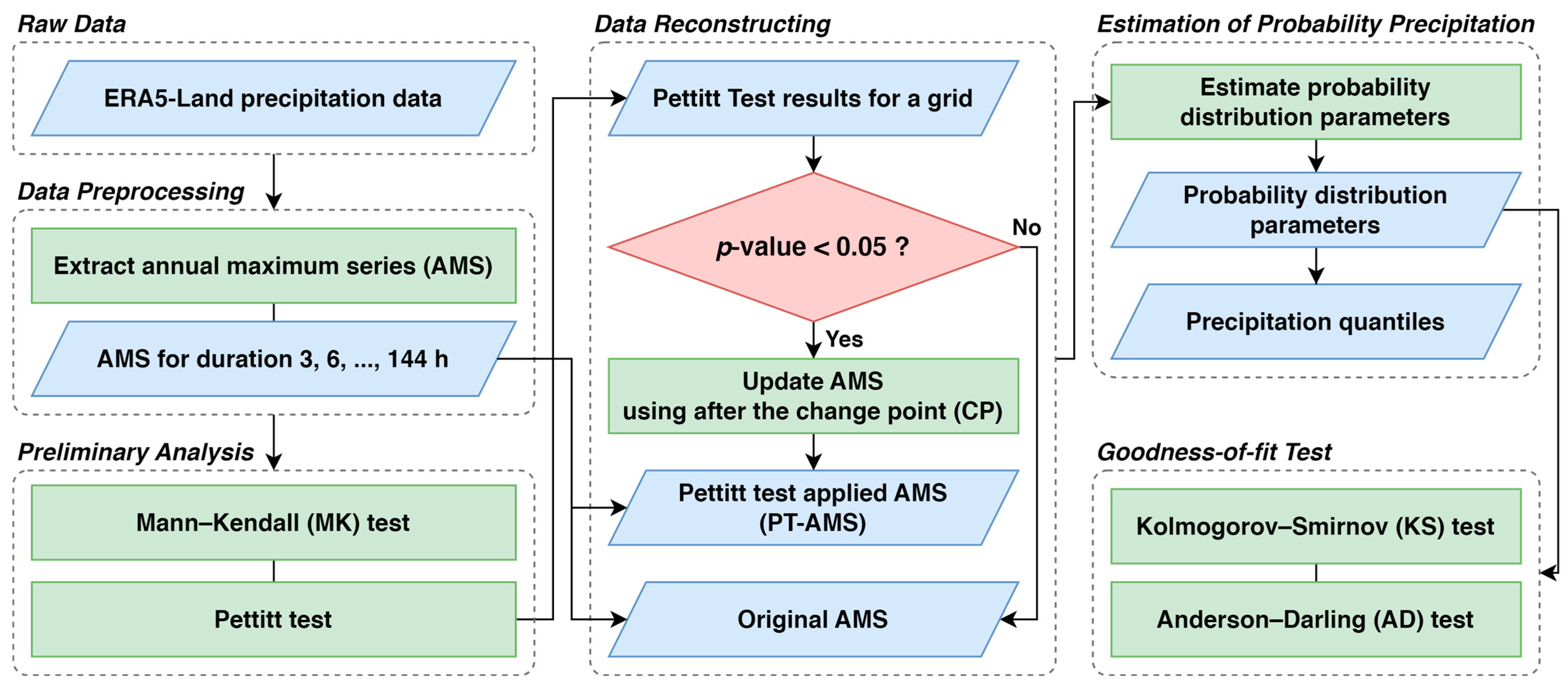
Figure 1 illustrates a flow chart of the analysis conducted in this study. A brief explanation of each part is as follows. First, the annual maximum series (AMS) is extracted for different durations from the ERA5-Land data. Using this, the MK test is performed to examine trends, followed by the Pettitt test. For significant results from the Pettitt test with a 5% significance level, the AMS is updated using only the data after the CP is identified by the Pettitt test (referred to as PT-AMS). For both datasets, probability distribution parameters are estimated, and the precipitation quantile is calculated. Finally, the goodness-of-fit is tested using two methods.
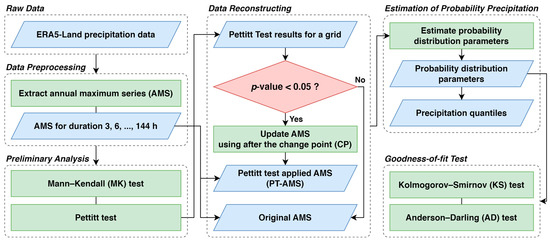
Figure 1.
Research framework for this study.
2.2. Mann–Kendall Test
Time series trend analysis techniques are generally divided into two categories: parametric and non-parametric approaches. Parametric methods involve assumptions about the distribution of the population, whereas non-parametric methods do not. Non-parametric methods are often more widely used compared to parametric methods because they can comprehensively analyze the relationships between all data points based on their ranks, allowing for flexibility in accounting for missing values and seasonality [17].
The MK test, one of the non-parametric methods, is a technique utilized to analyze whether there is an increasing or decreasing monotonic trend in time series data. The MK test, proposed by Mann [18] and Kendall [19], has a null hypothesis that no trend is present in the time series being analyzed. In this process, the statistic of the MK test () is defined as follows.
where is the -th value of the time series data, and is the -th value that comes after . The function is a sign function, which is defined as follows based on the difference between the two values.
In the MK test, represents the cumulative sum of positive rank differences (upward trend) and negative rank differences (downward trend) over time. Afterward, the -value is calculated, followed by the p-value, which is utilized to assess the significance. At a significance level of 0.05, if the p-value is greater than 0.05, the null hypothesis, indicating the absence of a trend, is accepted; otherwise, the alternative hypothesis is accepted. Typically, the MK test also calculates Sen’s slope [20], which quantifies the overall trend of the data by estimating the slope.
2.3. Pettitt Test
Among various methods, this study employs the non-parametric homogeneity test, the Pettitt test, which has been proven in previous studies to be one of the most reliable methods for detecting CPs or shifts in data [14,15,16]. The Pettitt test is an order-based non-parametric statistical test used to analyze deviations from homogeneity in time series data [21]. It can be seen as an extension of the Mann–Whitney U test [22]. Assuming that a sequence of variables has a CP at time and can be divided into two sets with different distribution functions ( and ), the hypotheses for the test are as follows.
where the null hypothesis () is that no CP is present, while the alternative hypothesis () is that a CP exists.
This method detects CPs in a time series as follows. First, assume there is a change at the -th point in the time series data . The data from to are considered the first segment, and the data from to are considered the second segment.
The rank-based Pettitt statistic is calculated as follows.
where is a rank-based statistic, which is defined as follows.
where is the sign function which is defined as follows depending on the value of .
Ultimately, through this series of steps, the point in time where the value of is maximized is determined as the final CP (). Based on asymptotic arguments regarding the test statistic, Pettitt [21] approximately defined the p-value for the Pettitt test as follows.
where is the total number of data, and is the test statistic at time . Typically, if the p-value is lower than a certain threshold (commonly 0.05), the null hypothesis is rejected, and the CP is considered statistically significant.
2.4. Estimation of Probability Precipitation Quantiles
Selecting an appropriate probability distribution is vital in precipitation frequency analysis. The generalized extreme value (GEV) distribution is one of the most widely utilized probability distributions for frequency analysis globally [23,24,25]. In addition to its role in hydrological studies, the GEV distribution is also widely applied in fields such as finance, climatology, the other branches of geosciences to model various extreme events [26,27,28,29]. GEV distribution comes in three types and has three parameters (location, scale, and shape). First, when the shape parameter is zero, extreme values have no upper and lower limit, and the distribution exhibits a relatively light tail. This is classified as type 1 and is referred to as GEV-I (also known as Gumbel distribution). When the shape parameter is positive, extreme values are bounded from below, and the distribution has a heavy tail. This is classified as type 2 and is called GEV-II (or the Fréchet distribution). Lastly, when the shape parameter is negative, extreme values are capped by an upper limit, and the distribution exhibits a short tail. This is classified as type 3, known as GEV-3 (or the Weibull distribution).
Among GEV models, the Gumbel distribution is among the most commonly used distributions for frequency analysis due to its simplicity, accuracy of estimated parameters, and practical reasons [30]. A recent report in Korea on estimating precipitation quantiles [31] also recognized the Gumbel distribution as the most suitable probability distribution for all observation stations managed by the Korea Meteorological Administration. In Korea, it was established to incorporate the Gumbel distribution for the precipitation frequency analysis in the Standard Guidelines for Flood Estimation [32]. Therefore, we used the Gumbel distribution for the precipitation frequency analysis in this study.
If refers to the precipitation quantiles (mm), the probability density function (PDF) and cumulative distribution function (CDF) of the Gumbel distribution can be expressed as follows:
where represents the location parameter, indicating where the maximum probability occurs, and denotes the scale parameter. Both and share the same units as .
The World Meteorological Organization (WMO) recommends the probability weighted moment (PWM) method as a suitable approach for parameter estimation in hydrological frequency analysis. This method is particularly noted for providing stable results when interpreting data series with shorter records, a common case in Korea [33]. Furthermore, the use of PWM is also advocated in Korea by many studies [32,34]. The detailed procedure for estimating Gumbel distribution parameters using PWM can be found in Lee et al. [5].
2.5. Goodness-of-Fit Test
2.5.1. Kolmogorov–Smirnov Test
The Kolmogorov–Smirnov test (KS test) measures the maximum difference between the empirical CDF (ECDF) of a given dataset and the cumulative distribution function (CDF) of an assumed distribution. It is suitable for continuous data and is often used for testing normality; however, it can be applied to other distributions as well. The KS test is non-parametric, meaning it can be used without prior assumptions about the distribution. Additionally, it is primarily sensitive to the central part of the distribution and less sensitive to extreme values (the tails).
where represents the KS statistic, which is the absolute maximum difference between the two distributions. refers to the CDF of the assumed distribution, and denotes the ECDF of the data. In the analysis, if the p-value exceeds 0.05, it is typically concluded that the data likely align with the assumed distribution.
2.5.2. Anderson–Darling Test
The Anderson–Darling test (AD test) is comparable to the KS test but is more sensitive to extreme values. It emphasizes the differences between the tails of the data and the assumed distribution. While it is primarily used for testing normality, it can also be applied to other distributions that are sensitive to extreme values. The test provides both test statistics and several critical values for different significance levels, allowing for flexible interpretation of the results.
where represents the CDF of the assumed distribution, and refers to the sample size of the data. Additionally, denotes the ordered data values. A smaller test statistic indicates that the data fit the assumed distribution better, and if the test statistic is less than the critical value at a specified significance level, the data are regarded as fitting the assumed distribution.
3. Data and Study Area
3.1. Precipitation Data
Satellite-based global reanalyzed precipitation data come in many forms, depending on the type of satellite and the algorithms that produce the data. They have different regional and spatial resolutions, periods, and temporal resolutions. Spatial resolutions range from as small as 0.04° to 2.5°, and temporal resolutions range from 1 h to 1 month. For spatial resolution, the coarsest possible resolution is required given the size of our country. In the case of temporal resolution, it seems necessary to consider the minimum resolution of 1 h, but there is a limitation that it is difficult to secure reanalysis data before 2000. Therefore, depending on the purpose of the analysis, it is necessary to consider a combination of these points to determine the appropriate reanalyzed precipitation data [5]. In this regard, Kim and Lee [35] compared three analyses, NCEP2, JRA55, CRU, and ERA5, with gridded data from CRU using correlation coefficients, difference statistics (Bias and RMSE), and Taylor diagrams for precipitation over East Asia, including the Korean Peninsula, and found that ERA5 performed the best. Furthermore, the ERA5-Land data have a finer resolution of 9 km than ERA5, which has a resolution of 31 km. This advantage makes ERA5-Land well suited for regions with complex topography and climate, such as the Korean Peninsula. In addition, ERA5-Land has a temporal resolution of 1 h and provides more than 70 years of data since 1950, making it the most suitable reanalyzed precipitation data for this study.
Thus, we utilized ERA5-Land data for our analysis. ERA5-Land is a global reanalysis dataset with high spatial resolution [36]. It provides detailed information on surface variables such as temperature, precipitation, relative humidity, and soil moisture. ERA5-Land has been validated for accuracy, offering a spatial resolution of 9 km and an hourly temporal resolution, and the data have been gridded again to a consistent latitude and longitude grid with a resolution of 0.1°. ERA5-Land offers comprehensive and consistent historical data from 1950 to the present, and this dataset is widely used across various applications worldwide [37,38,39]. Due to missing data in the early 1950s during the conversion to Korean time, we used hourly precipitation data from 1951 to 2023, covering a total of 73 years for this study.
3.2. Study Area
The study area is the Korean Peninsula, roughly located between latitudes 33° and 43° and longitudes 124° and 131°. Figure 2 shows the location of the study area and a digital elevation model of the Korean Peninsula. The region is mainly classified as a temperate climate zone with four distinct seasons. Spring and fall are characterized by clear and dry weather due to the influence of migratory high-pressure systems. In contrast, summer is marked by hot, humid weather due to the North Pacific high, while winter is generally cold and dry, influenced by continental high-pressure systems. Precipitation is concentrated in the summer, with monsoons and typhoons, while winter is marked by cold weather and relatively low precipitation. Additionally, approximately 70% of the Korean Peninsula is mountainous, with the terrain divided into eastern and western regions by mountain ranges.
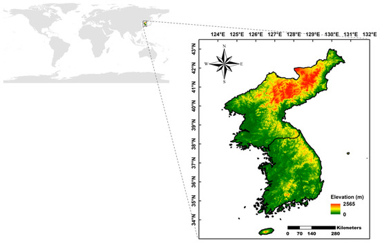
Figure 2.
Location and digital elevation model (m) of study area.
4. Results
4.1. Trend from Mann–Kendall Test
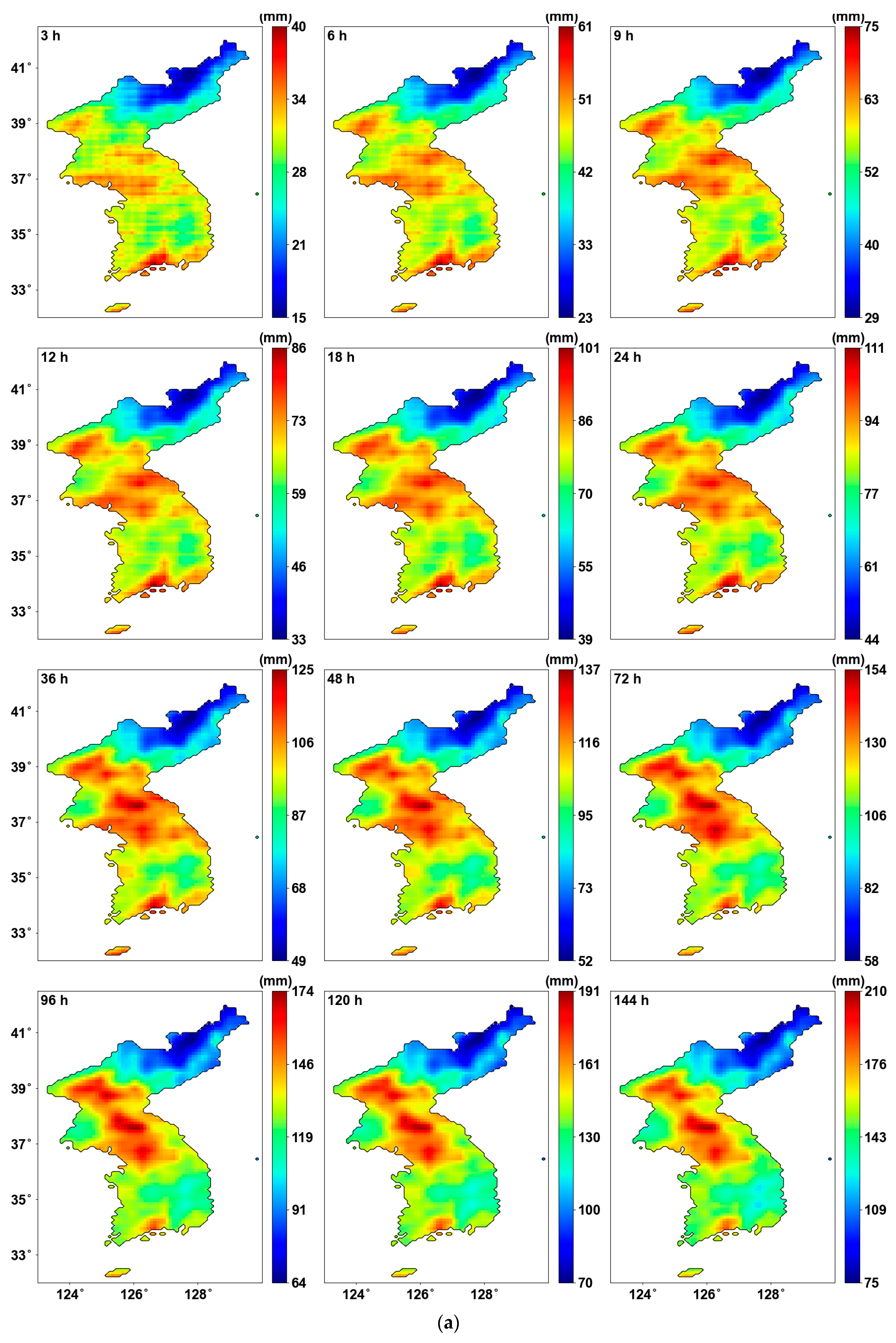
Figure 3 illustrates the average of AMS for all years and the results of the MK test for all durations. First, Figure 3a shows the average AMS. The central and southern regions of the Korean Peninsula show higher average AMS, whereas lower average AMS are noted in the northeastern areas. Figure 3b shows the results of the MK test for the entire region. In general, North Korea shows a decreasing trend, while South Korea shows an increasing trend. Additionally, as the duration increases, the changes in increase or decrease become more distinct. In the central region of the Korean Peninsula, an increasing trend begins to appear from the 48 h duration onwards. Figure 3c highlights only the areas where the p-value is below 0.05, using a new color bar. It can be observed that all significant areas exhibit an increasing trend. In most durations, the southeastern region of South Korea shows a significant increase. While regional differences are evident for most durations, the 72 and 96 h durations, representing 3- and 4-day AMS, show a consistent increase across the entire southeastern region. The southernmost region displays a continuous increasing pattern, with the rate of increase becoming larger as the duration extends. However, it is challenging to accurately determine the CP of the AMS based solely on this trend analysis.
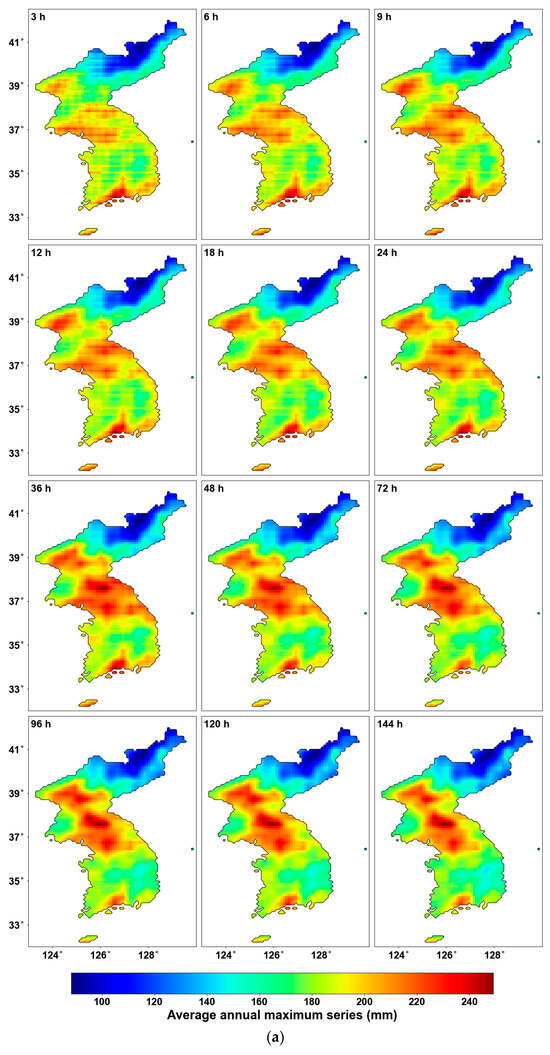

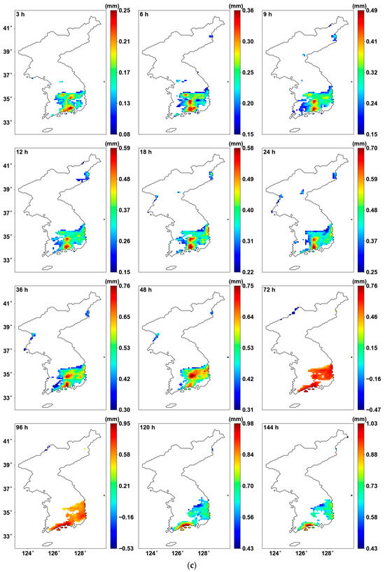
Figure 3.
Mean AMS and MK test results: (a) average AMS; (b) Sen’s slope for all grids; (c) Sen’s slope for the grid with p-value < 0.05.
4.2. Homogeneity from Pettitt Test
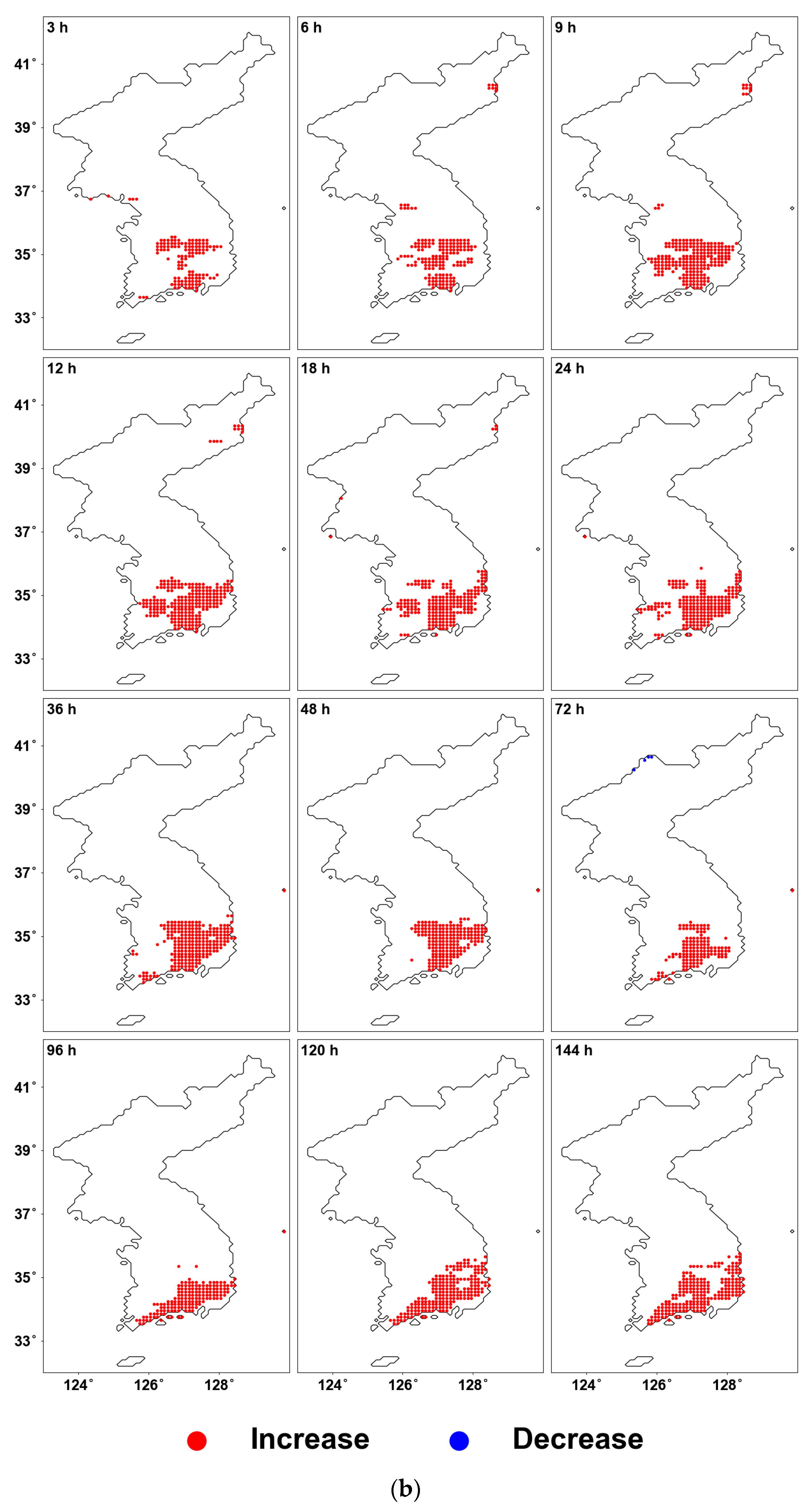
Figure 4 illustrates the results of the Pettitt test, highlighting only the significant areas (p-value < 0.05). As seen in Figure 4a, the grids with significant changes are mostly concentrated in the southeastern part of South Korea, similar to the previous results from the MK test, and the CPs are concentrated around the 1970s. There is a trend where the CP shifts more recently as the duration decreases. Figure 4b shows the increase and decrease based on the averages before and after the CP, and it can be observed that almost all regions exhibit an increasing trend.
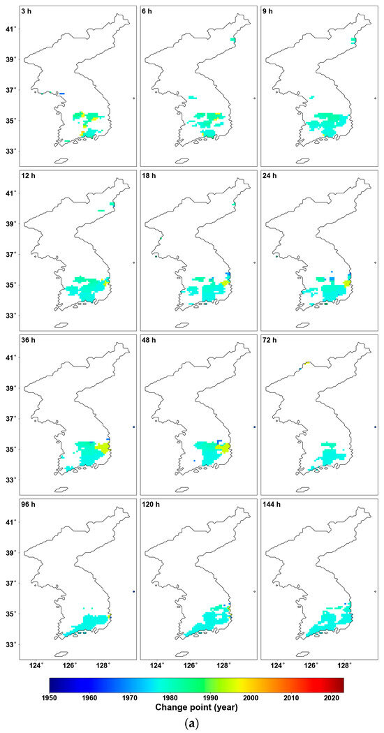
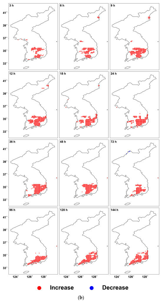
Figure 4.
Pettitt test results: (a) CP for the grid with p-value < 0.05; (b) shift in mean before and after CP for the grid with p-value < 0.05.
Table 1 shows the proportion of significant areas by duration. The proportion varies between a low of 5.8% and a high of 10.4%, with an average of about 8.6% of the areas experiencing changes in homogeneity. When the scope is limited to South Korea, approximately one-sixth of the region experienced such changes. This significant proportion further emphasizes the importance of assessing homogeneity.

Table 1.
Percentage of grids with significant homogeneity changes observed.
4.3. Estimation of Probability Distribution Parameters Considering Homogeneity from Pettitt Test
Figure 5 shows the results of estimating the probability distribution parameters using the original AMS. Overall, the patterns of the location parameter and scale parameter appear very similar, as seen in the average AMS. The central and southern parts of the Korean Peninsula exhibit stronger intensities, while weaker intensities are observed in the mountainous areas in the northeast. This suggests that the central and southern parts of the Korean Peninsula experience relatively higher precipitation, with greater variability in precipitation and a higher likelihood of extreme precipitation events.
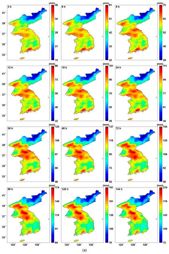
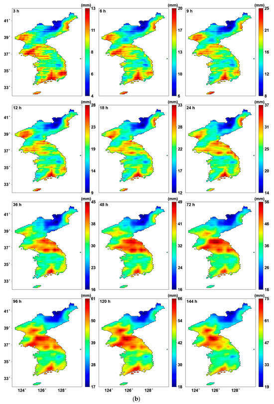
Figure 5.
Probability distribution parameters using original AMS: (a) location parameters (mm); (b) scale parameters (mm).
Figure 6 shows the results after applying PT-AMS. By reconstructing the data for the southern regions, the overall AMS increased, leading to changes in the parameters as well. The location parameter in Figure 6a generally shows an increase, while the scale parameter in Figure 6b shows no significant difference.

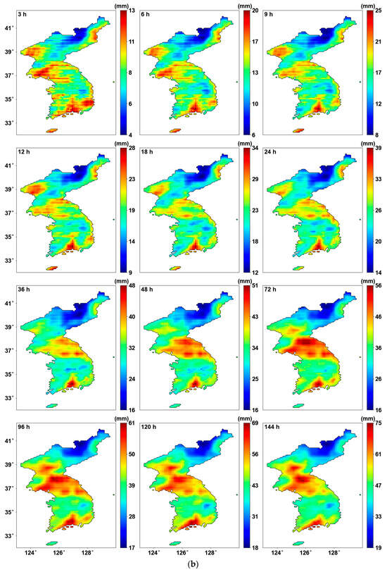
Figure 6.
Probability distribution parameters using PT-AMS: (a) location parameters (mm); (b) scale parameters (mm).
4.4. Precipitation Quantiles
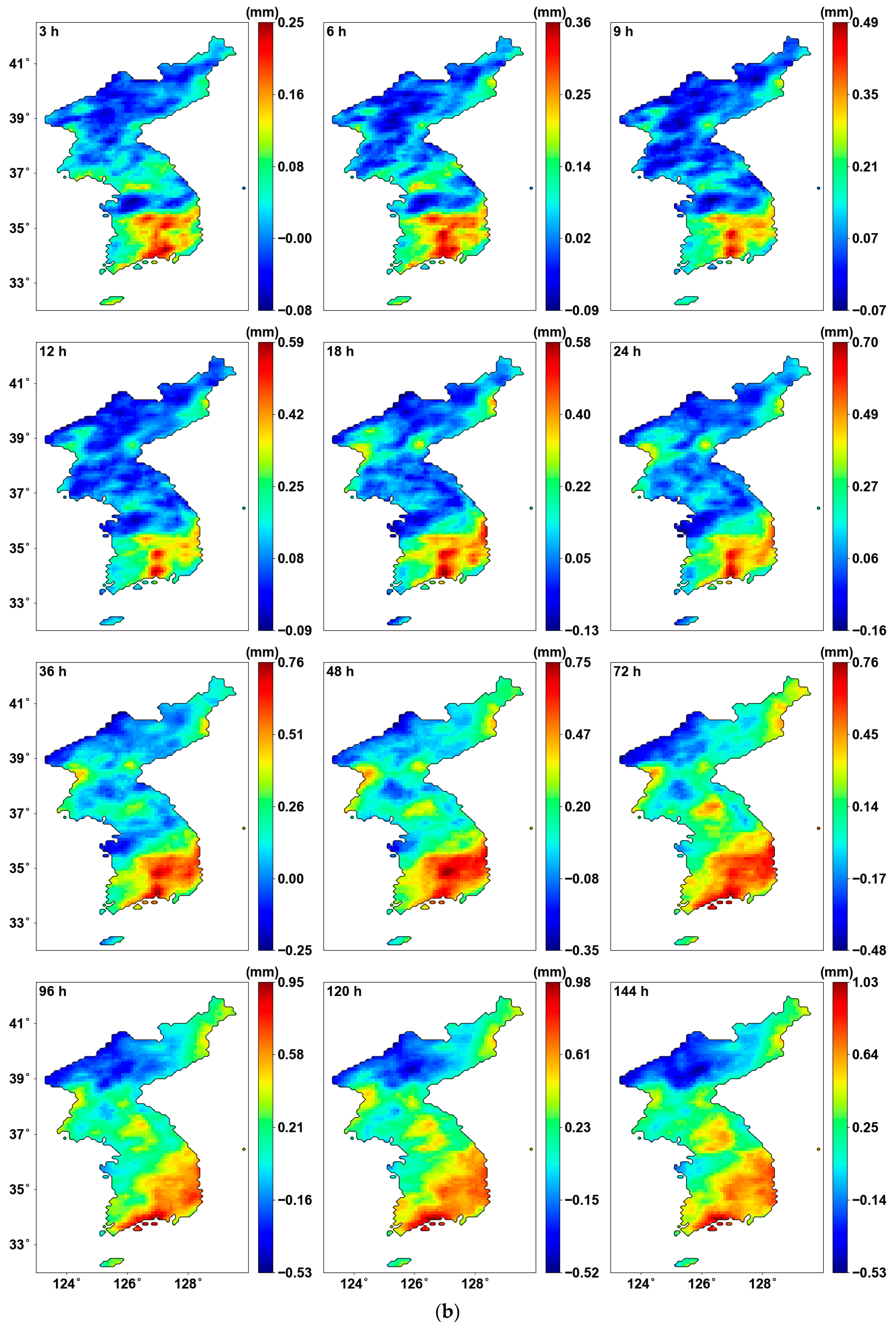
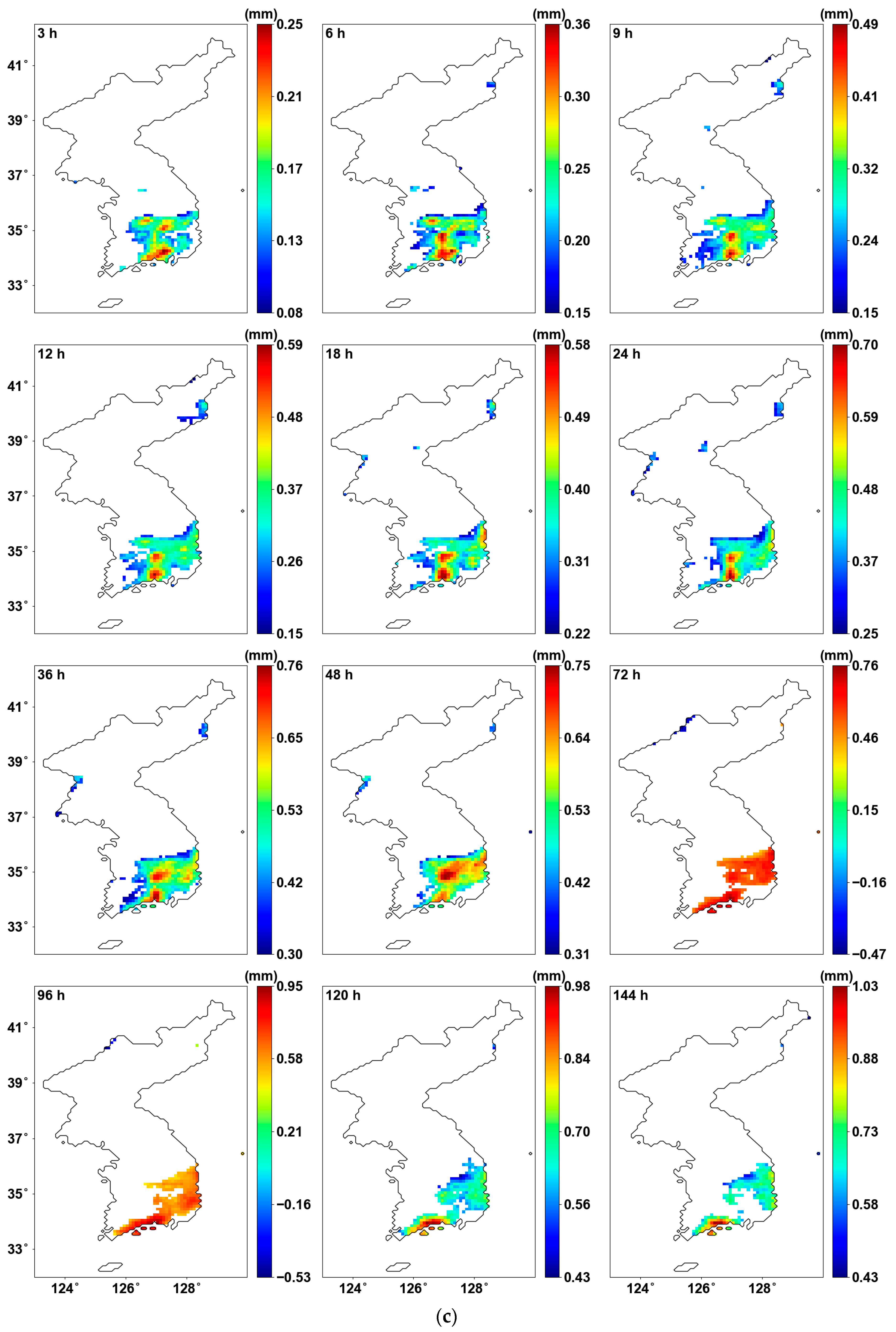
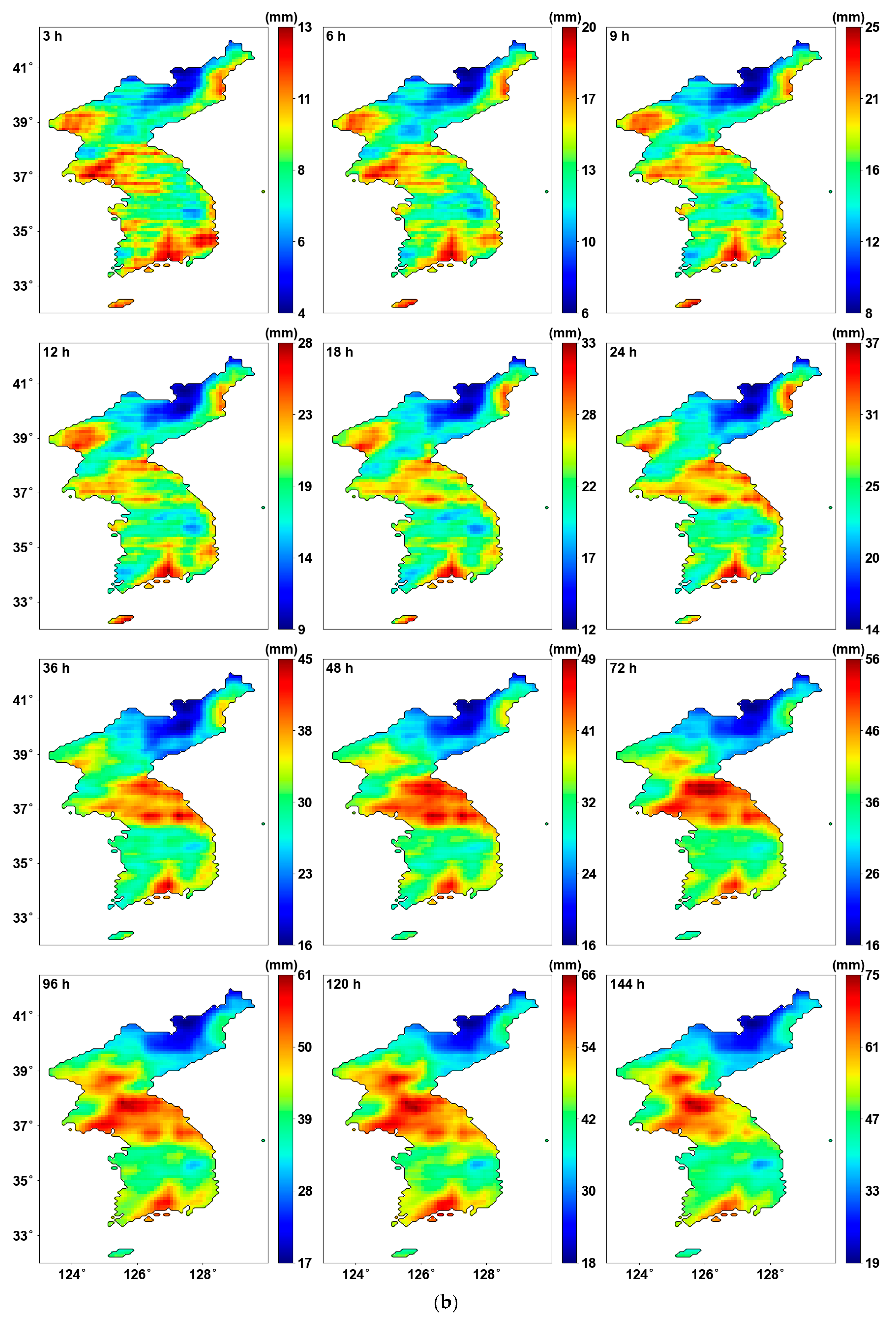
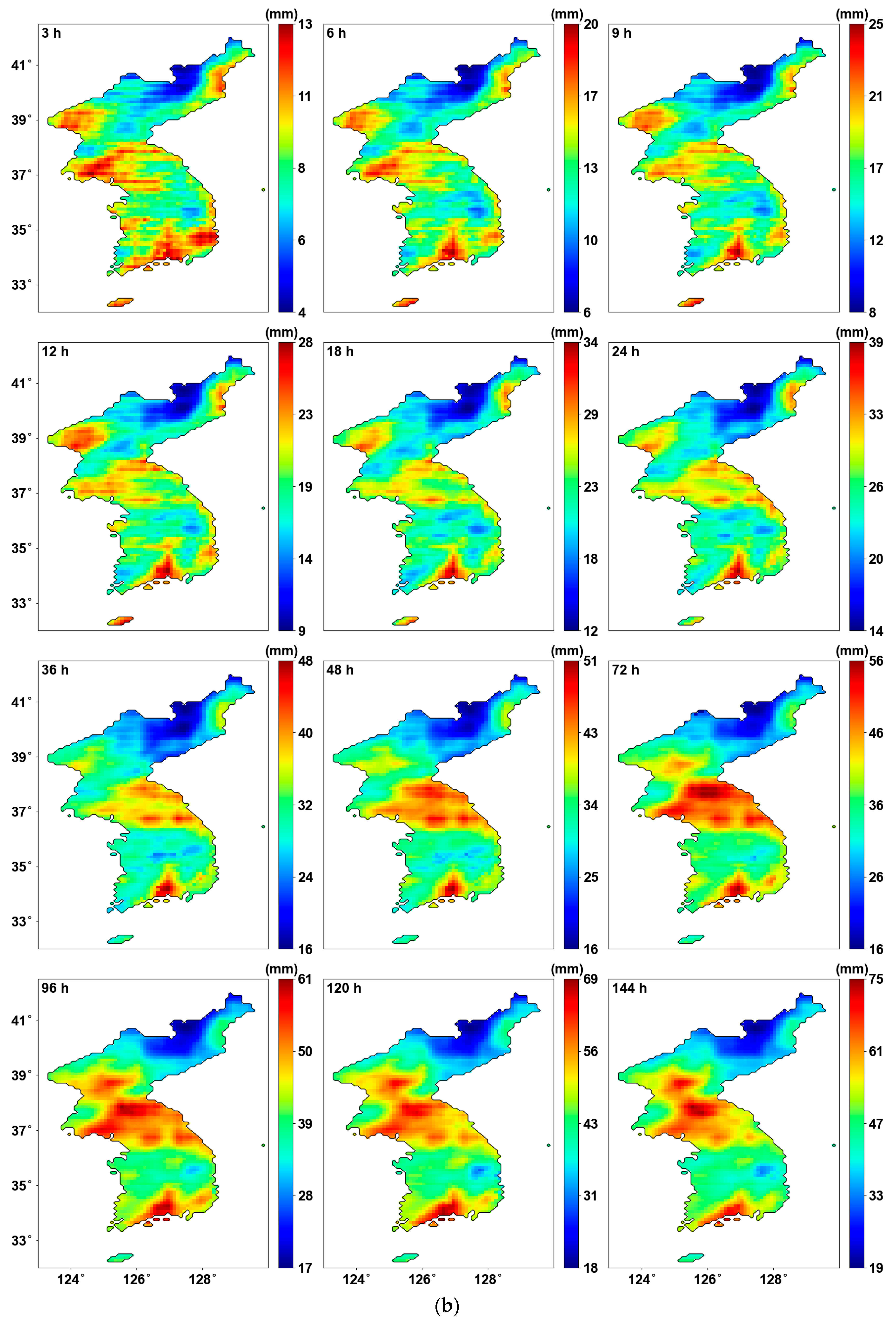
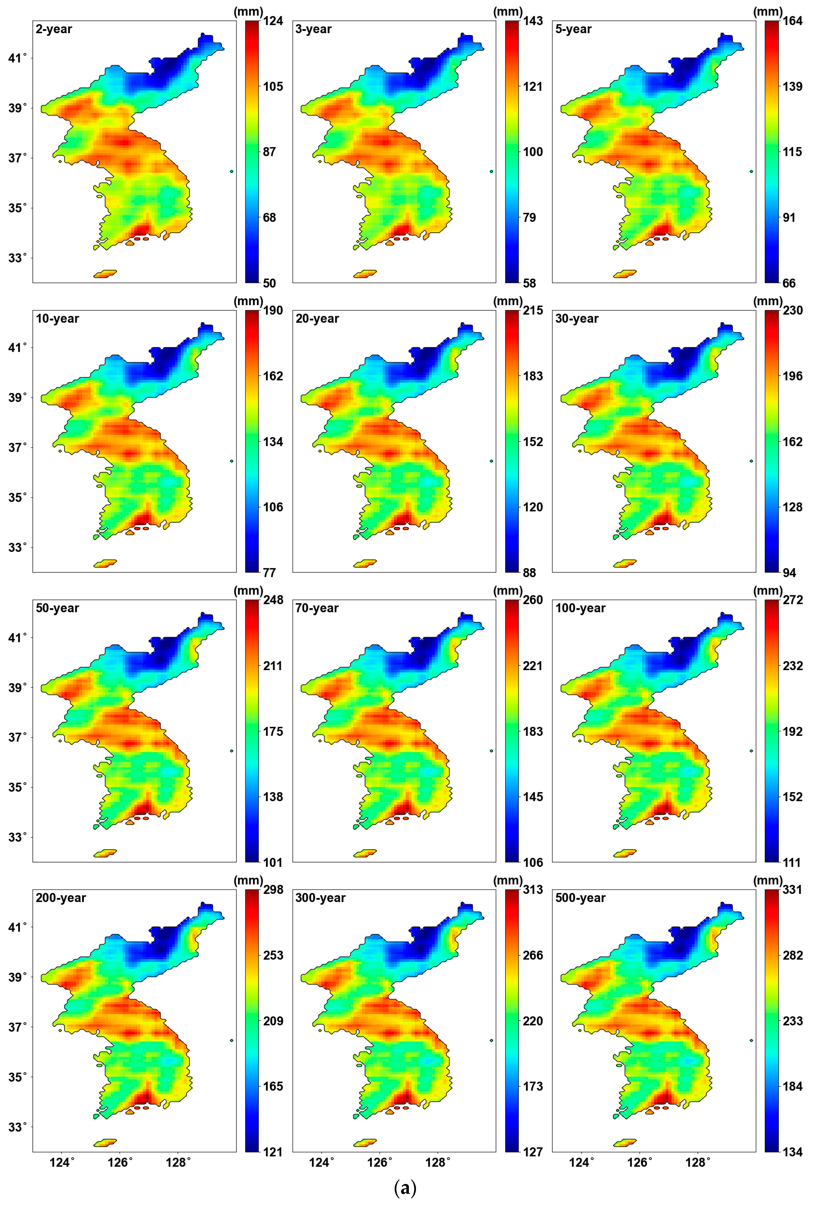
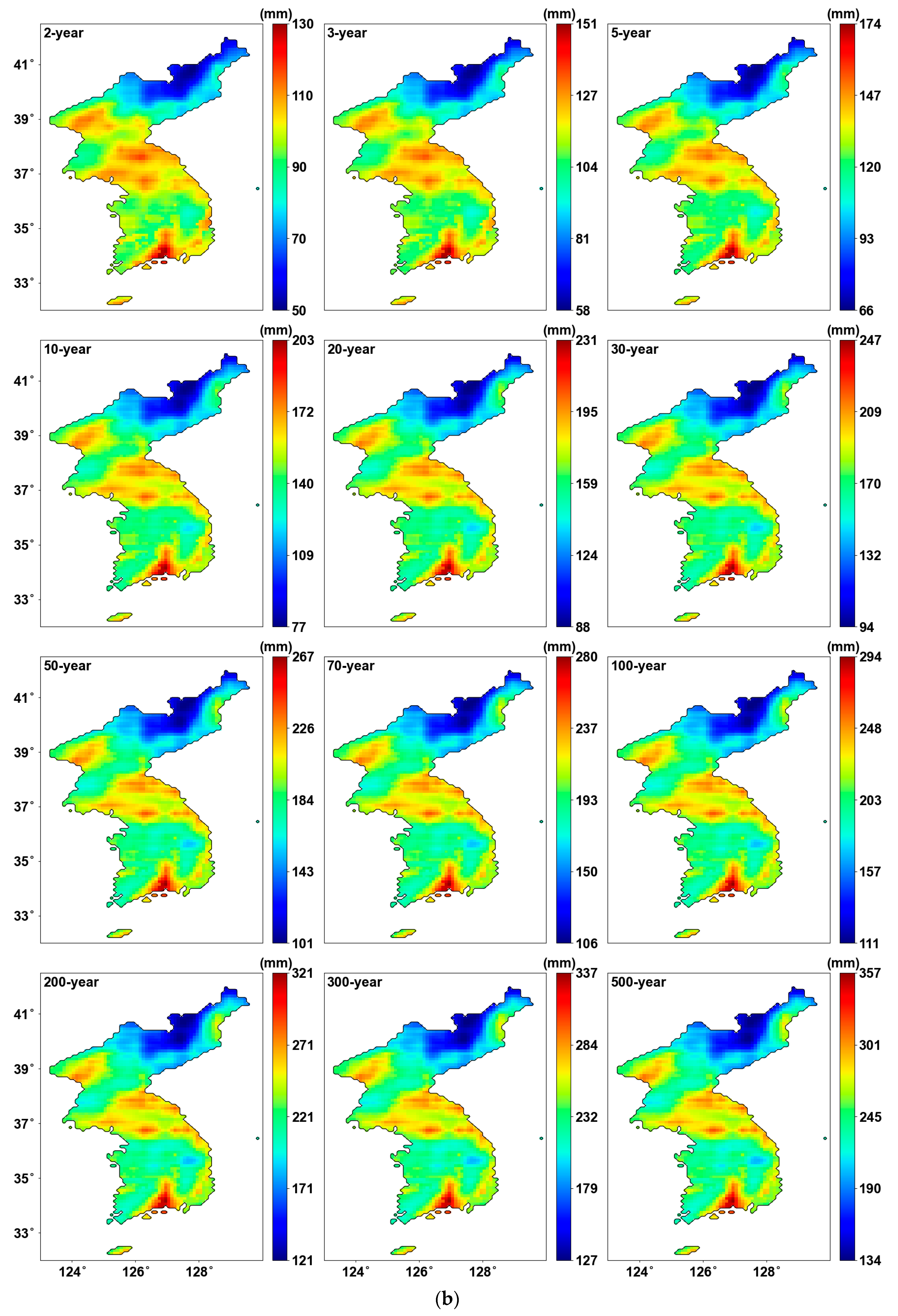
Figure 7 shows the precipitation quantile estimated using the probability distribution parameters. We can see that the maximum values are updated for each return period, leading to an expanded range in the color bar when using PT-AMS compared to the original AMS. In other words, the most extreme precipitation quantile was produced from the grids where the PT-AMS was used, as shown in Figure 7b. Consequently, the central region of the southernmost area becomes more prominent.
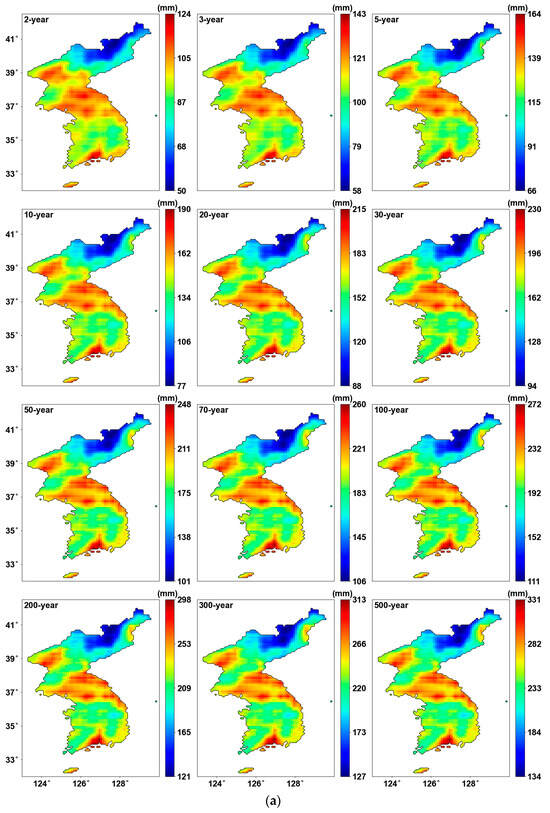
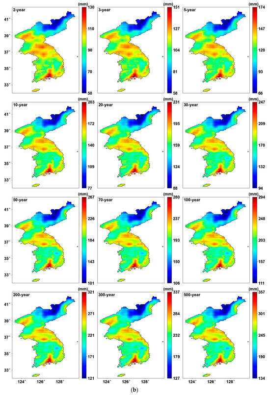
Figure 7.
Precipitation quantile (mm) for 24 h duration: (a) result from original AMS; (b) result from PT-AMS.
5. Discussions
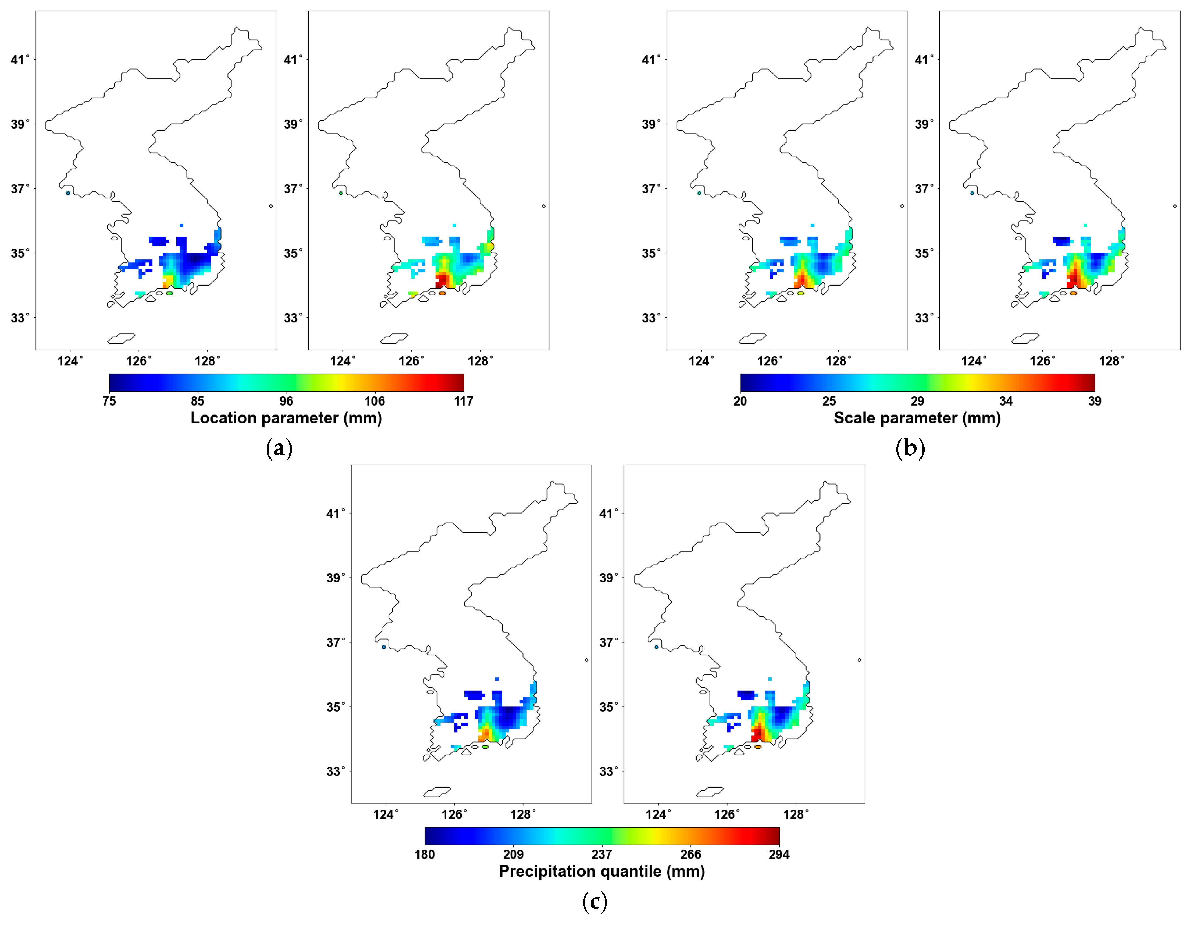
In the discussion section, we aim to focus on the regions where changes occurred and perform a comparison. We compared the basic parameters, the precipitation quantile, and additionally conducted a goodness-of-fit test for the parameters. First, Figure 8 illustrates the analysis results where the original AMS (left) and the PT-AMS (right) were used. The location parameter in Figure 8a shows a greater change compared to the scale parameter in Figure 8b. This indicates that the change in AMS is more related to an overall shift in the mean rather than a change in the variance. The 100-year 24 h precipitation quantile shown in Figure 8c reflects this influence of the location parameter, resulting in an overall increase in values. This implies that the increase in precipitation amounts has a greater impact on extreme precipitation events in the region than precipitation variability.

Figure 8.
Probability distribution parameters for 24 h duration and precipitation quantile using (left) original AMS and (right) PT-AMS: (a) location parameter (mm); (b) scale parameter (mm); (c) 100-year 24 h precipitation quantile (mm).
All analyses involving probability distribution parameters and precipitation quantiles, including the MK test, found that only the southernmost part of the peninsula experienced significant changes in precipitation characteristics. There are several possible explanations for this. First, the variability in the North Pacific High could be a major contributor. Since the AMS primarily occurs in the summer, the calculated probabilistic rainfall is also influenced by summer rainfall patterns. The southern part of the Korean Peninsula is most affected by the North Pacific High during summer. If the position or intensity of this high-pressure system changes, it can lead to altered rainfall patterns in the region. This phenomenon is closely related to the monsoon front. The monsoon front is the boundary between two air masses, typically characterized by a significant temperature difference, which can trigger intense rainfall. When the northward expansion of the North Pacific High is delayed, the monsoon tends to last longer. Additionally, while the southern region has relatively flat terrain, the coastline, especially around the southern coast, is complex and irregular. This topography allows for greater influence from moist air masses coming from the sea, which can lead to variations in rainfall characteristics. Besides these factors, it is also hypothesized that climate change, urbanization, and other interwoven influences may have contributed to the changes in rainfall patterns in the region.
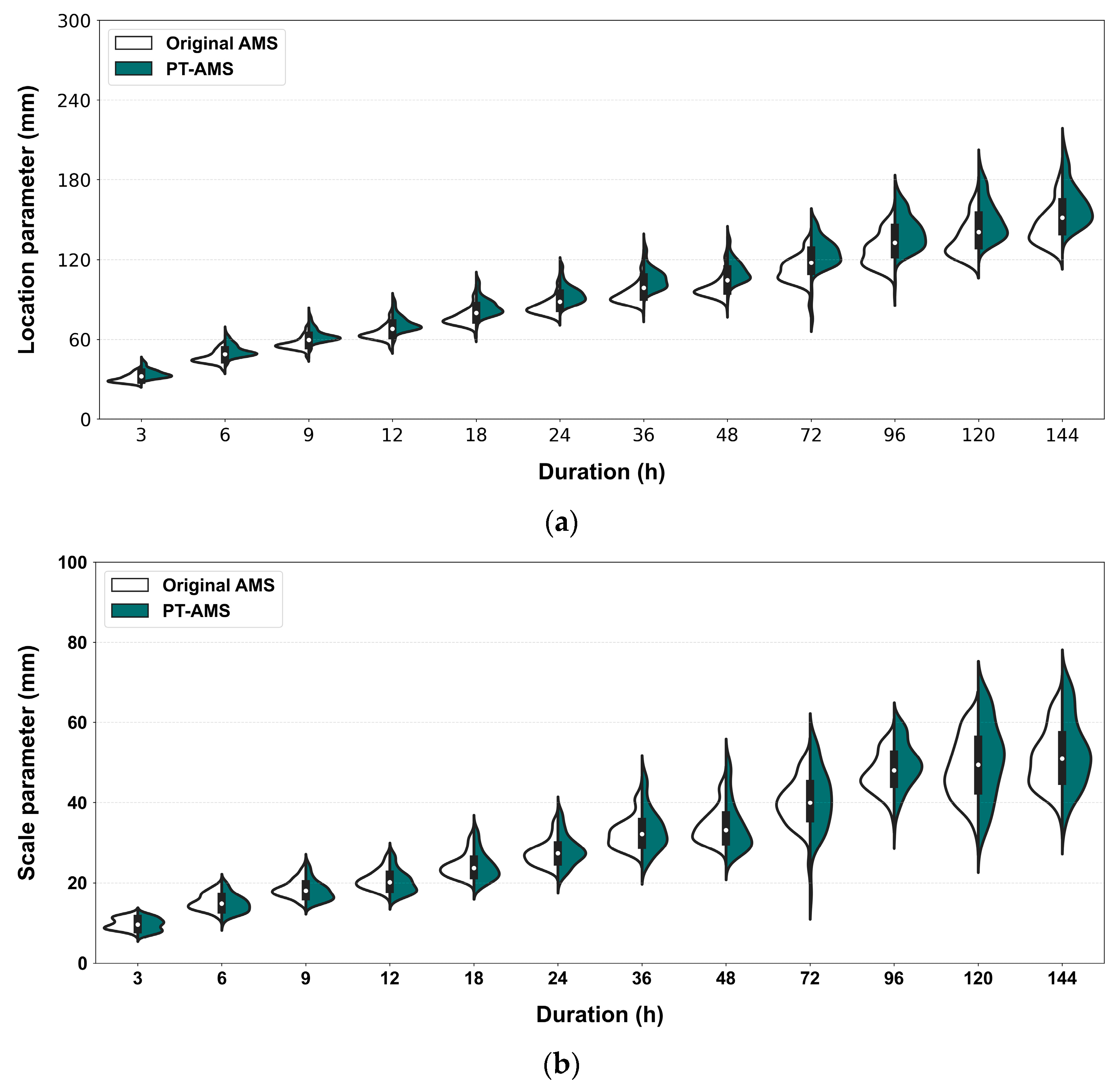
Figure 9 compares the original AMS results and PT-AMS results for regions with p < 0.05 using violin plots. A violin plot represents the distribution of continuous data by combining a box plot and a kernel density curve. The curves on either side illustrate the distribution of each dataset, while the box in the center can be interpreted like a regular box plot. As observed earlier, the increase in the location parameter is more pronounced in Figure 9a, while no significant difference is seen in the scale parameter in Figure 9b. When looking at the distribution, the PT-AMS results show a somewhat simplified distribution compared to the original AMS. Considering that most of these regions are similar, it can be argued that the latter result is more reasonable; however, quantifying this is difficult.
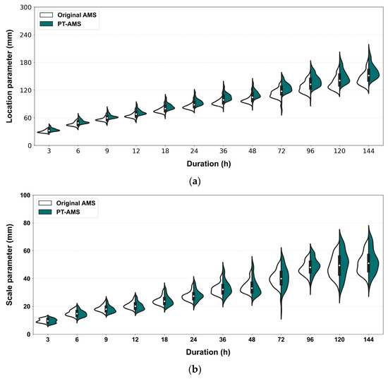
Figure 9.
Probability distribution parameters using original AMS and PT-AMS: (a) location parameter (mm); (b) scale parameter (mm).
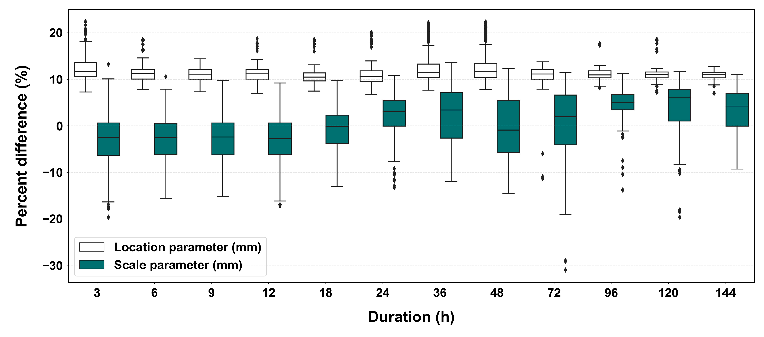
Figure 10 is a graph comparing the differences between the two cases. It shows the percentage change in the parameters when PT-AMS is applied compared to the results from the original AMS. The location parameter shows an increase of about 10%, while the scale parameter tends to slightly decrease for shorter durations and slightly increase for longer durations. This indicates that while the average of the AMS changes, the variance does not fluctuate significantly.
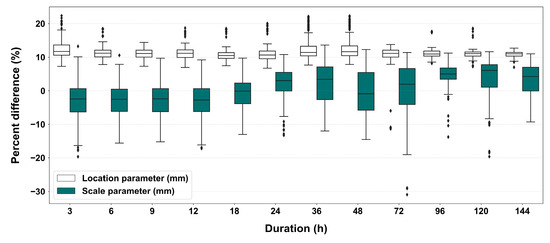
Figure 10.
Box plots representing the percent difference of the probability distribution parameters using the PT- AMS to the probability distribution parameters using the original AMS. The diamond shapes indicate outliers.
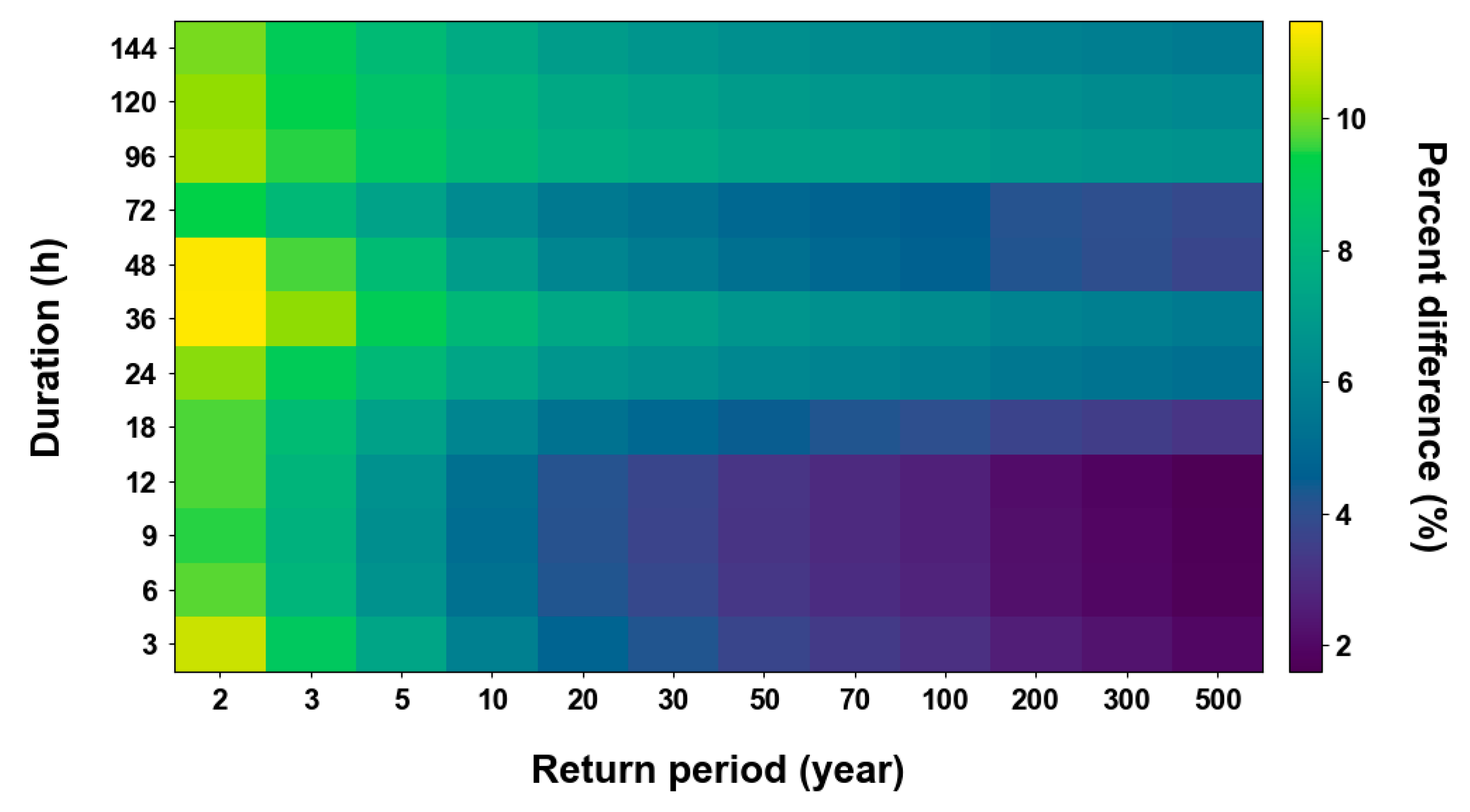
Figure 11 shows the average relative percentage difference for all grids with a significant change in the precipitation quantile calculated by utilizing the parameters. The differences tend to be larger for shorter return periods. The largest difference occurs for a 2-year return period and a 36 h duration, with a difference of approximately +11.5%.
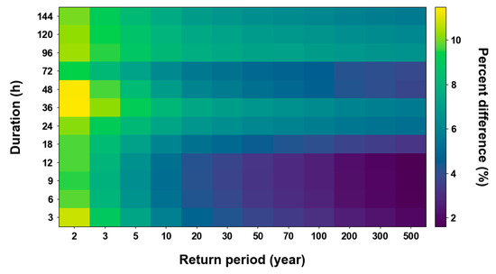
Figure 11.
Percent difference of the precipitation quantile using PT-AMS to the precipitation quantile using original AMS.
Figure 12 shows the results of examining the goodness-of-fit of these distributions using the KS test and AD test. Based on the KS test results in Figure 12a, there are slight differences depending on the duration. However, in both the case of using the original data and the Pettitt test results, all cases have p > 0.05, indicating that the data fit the assumed distribution.
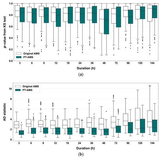
Figure 12.
Goodness-of-fit test results for the probability distribution: (a) p-value obtained from the KS test; (b) statistic from the AD test. The diamond shapes indicate outliers.
Figure 12b compares the AD test statistics using a box plot. When the significance level is set at 5%, the critical values are 0.740 for the original AMS and 0.735 for PT-AMS. Only a few cases when the PT-AMS was applied passed the threshold. However, as seen in the overall distribution, using only recent homogeneous data through the Pettitt test yields much better statistical values than the cases using the original AMS. This implies that the updated Gumbel distribution’s location parameter and scale parameter were better estimated, indicating that the distribution more accurately captures the precipitation variability and mean precipitation for each region. Thus, the methodology proposed in this study provides more reasonable results compared to traditional methods.
It will be necessary to examine aspects related to spatial resolution in more detail. The ERA5-Land data provide a grid average with a resolution of 9 km by 9 km. As a result, it may not capture the fine-scale variability of precipitation occurring in small areas, leading to a spatial smoothing effect on precipitation [40]. Consequently, extreme values may be diluted, causing the precipitation quantile to be smaller than what would be obtained through at-site frequency analysis. This is the opposite concept of the areal reduction factor needed when expanding point results to an area [41]. Since the size of the grid used in ERA5-Land data may differ from the actual area of interest for estimating precipitation quantiles, it will be necessary to consider a series of conversion factors when applying the results of this study to larger or smaller areas.
Another important aspect in estimating precipitation quantiles is that the distribution should effectively capture skewed events in order to accurately interpret extreme hydrological phenomena. In other words, it must appropriately represent the skewness of the given sample data, and the shape parameter, which is related to skewness, plays a crucial role. In this study, the Gumbel distribution was solely used for estimating precipitation quantiles in the region. However, the Gumbel distribution lacks a shape parameter, limiting its ability to account for various types of precipitation events. Therefore, by considering the GEV distribution, which is widely used for extreme events due to its shape parameter, a more diverse approach can be taken, allowing for more reasonable estimates of precipitation extremes.
6. Conclusions
In this study, grid-based precipitation quantiles for the Korean Peninsula were estimated, considering the homogeneity of the annual maximum series using long-term gridded reanalysis precipitation data. For regions where statistically significant changes in homogeneity were observed, precipitation quantiles were recalculated using only the data after the CP, and the results were compared with those from regions without such changes. The key conclusions of this study are summarized as follows.
- (1)
- The trend analysis conducted as a preliminary step using the MK test showed a significant increasing trend in the southeastern region of Korea. Homogeneity analysis through the Pettitt test also revealed changes in homogeneity with increasing trends in similar areas. The proportion of affected grid cells was approximately 8.6% of the total.
- (2)
- The parameters of the Gumbel distribution estimated using the original AMS, and the resulting precipitation quantiles generally showed stronger values in the central and southern parts of the Korean Peninsula, while weaker values were observed in the northeastern region.
- (3)
- The frequency analysis performed using PT-AMS showed significant changes in the location parameter, with all values increasing. For the scale parameter, there was a slight decrease for shorter durations, but as the duration increased, a slight upward trend was observed. The resulting precipitation quantiles were largest for a return period of 2 years and a duration of 36 h, with an average increase of approximately +11.5%.
- (4)
- The goodness-of-fit test results showed no significant differences before and after, with all p-values exceeding 0.05 in the KS test. However, the AD test statistics indicated an improvement in fit.
We proposed a method to estimate precipitation quantiles more reasonably through the examination of homogeneity, and this was applied to the Korean Peninsula. The results obtained from this study are anticipated to function as meaningful foundational data for the design of hydraulic structures in areas where acquiring long-term ground observation data is challenging. Recently, research utilizing non-stationary frequency analysis, which incorporates a time component in the distribution to account for climate change, has been widely used. Future research could build on the results of this study by conducting non-stationary frequency analysis that considers the statistically significant CPs in the long-term annual maximum series, thereby providing a more reasonable estimation of precipitation quantiles.
Author Contributions
Conceptualization, S.O. and E.H.L.; data curation, J.B.; formal analysis, J.L.; investigation, C.J.; writing—original draft preparation, S.O.; writing—review and editing, E.H.L., J.S. and J.L. All authors have read and agreed to the published version of the manuscript.
Funding
This work was supported by the National Research Foundation of Korea (NRF) grant funded by the Korea government (MSIT) (No. NRF-2022R1A4A3032838) and under the KICT Research Program (project no. 20240166-001, Development of IWRM-Korea Technical Convergence Platform Based on Digital New Deal (3/3)) funded by the Ministry of Science and ICT.
Institutional Review Board Statement
Not applicable.
Informed Consent Statement
Not applicable.
Data Availability Statement
The raw data supporting the conclusions of this article will be made available by the authors on request.
Conflicts of Interest
The authors declare no conflicts of interest.
References
- Hosking, J.R.M.; Wallis, J.R. Regional Frequency Analysis: An Approach Based on L-Moments; Cambridge University Press: Cambridge, UK, 1997; ISBN 978-0-521-43045-6. [Google Scholar]
- Wang, Z.; Zeng, Z.; Lai, C.; Lin, W.; Wu, X.; Chen, X. A regional frequency analysis of precipitation extremes in Mainland China with fuzzy C-means and L-moments approaches. Int. J. Climatol. 2017, 37, 429–444. [Google Scholar] [CrossRef]
- Darwish, M.M.; Fowler, H.J.; Blenkinsop, S.; Tye, M.R. A regional frequency analysis of UK sub-daily extreme precipitation and assessment of their seasonality. Int. J. Climatol. 2018, 38, 4758–4776. [Google Scholar] [CrossRef]
- Forestieri, A.; Lo Conti, F.; Blenkinsop, S.; Cannarozzo, M.; Fowler, H.J.; Noto, L.V. Regional frequency analysis of extreme rainfall in Sicily (Italy). Int. J. Climatol. 2018, 38, e698–e716. [Google Scholar] [CrossRef]
- Lee, J.; Jun, C.; Kim, H.-J.; Byun, J.; Baik, J. Estimation of grid-type precipitation quantile using satellite based re-analysis precipitation data in Korean peninsula. J. Korea Water Resour. Assoc. 2022, 55, 447–459. [Google Scholar] [CrossRef]
- Heo, J.-H.; Kim, H. Regional frequency analysis for stationary and nonstationary hydrological data. J. Korea Water Resour. Assoc. 2019, 52, 657–669. [Google Scholar] [CrossRef]
- Nandakumar, N. Estimation of Extreme Rainfalls for Victoria: Application of the Forge Method; Cooperative Research Centre for Catchment Hydrology: Melbourne, VIC, Australia, 1995. [Google Scholar]
- Schaefer, M.G. Regional analyses of precipitation annual maxima in Washington State. Water Resour. Res. 1990, 26, 119–131. [Google Scholar] [CrossRef]
- Courty, L.G.; Wilby, R.L.; Hillier, J.K.; Slater, L.J. Intensity-duration-frequency curves at the global scale. Environ. Res. Lett. 2019, 14, 084045. [Google Scholar] [CrossRef]
- Gado, T.A.; Hsu, K.; Sorooshian, S. Rainfall frequency analysis for ungauged sites using satellite precipitation products. J. Hydrol. 2017, 554, 646–655. [Google Scholar] [CrossRef]
- Yoo, C.; Lee, J.; Ro, Y. Markov Chain Decomposition of Monthly Rainfall into Daily Rainfall: Evaluation of Climate Change Impact. Adv. Meteorol. 2016, 1, 7957490. [Google Scholar] [CrossRef]
- Sung, J.H.; Kim, Y.-O.; Jeon, J.-J. Application of distribution-free nonstationary regional frequency analysis based on L-moments. Theor. Appl. Climatol. 2017, 133, 1219–1233. [Google Scholar] [CrossRef]
- Kim, H.; Shin, J.-Y.; Kim, T.; Kim, S.; Heo, J.-H. Regional frequency analysis of extreme precipitation based on a nonstationary population index flood method. Adv. Water Resour. 2020, 146, 103757. [Google Scholar] [CrossRef]
- Wijngaard, J.B.; Klein Tank, A.M.G.; Können, G.P. Homogeneity of 20th century European daily temperature and precipitation series. Int. J. Climatol. 2003, 23, 679–692. [Google Scholar] [CrossRef]
- Costa, A.C.; Soares, A. Homogenization of Climate Data: Review and New Perspectives Using Geostatistics. Math. Geosci. 2008, 41, 291–305. [Google Scholar] [CrossRef]
- Hurtado, S.I.; Zaninelli, P.G.; Agosta, E.A. A multi-breakpoint methodology to detect changes in climatic time series. An application to wet season precipitation in subtropical Argentina. Atmos. Res. 2020, 241, 104955. [Google Scholar] [CrossRef]
- Hirsch, R.M.; Slack, J.R.; Smith, R.A. Techniques of trend analysis for monthly water quality data. Water Resour. Res. 1982, 18, 107–121. [Google Scholar] [CrossRef]
- Mann, H.B. Nonparametric tests against trend. Econom. J. Econom. Soc. 1945, 13, 245–259. [Google Scholar] [CrossRef]
- Kendall, M.G. Rank Correlation Methods; Charles Griffin: London, UK, 1975. [Google Scholar]
- Sen, P.K. Estimates of the Regression Coefficient Based on Kendall’s Tau. J. Am. Stat. Assoc. 1968, 63, 1379–1389. [Google Scholar] [CrossRef]
- Pettitt, A.N. A Non-Parametric Approach to the Change-Point Problem. J. R. Stat. Soc. C Appl. Stat. 1979, 28, 126–135. [Google Scholar] [CrossRef]
- Mann, H.B.; Whitney, D.R. On a test of whether one of two random variables is stochastically larger than the other. Ann. Math. Stat. 1947, 18, 50–60. [Google Scholar] [CrossRef]
- Fowler, H.J.; Kilsby, C.G. A regional frequency analysis of United Kingdom extreme rainfall from 1961 to 2000. Int. J. Climatol. 2003, 23, 1313–1334. [Google Scholar] [CrossRef]
- Overeem, A.; Buishand, A.; Holleman, I. Rainfall depth-duration-frequency curves and their uncertainties. J. Hydrol. 2008, 348, 124–134. [Google Scholar] [CrossRef]
- Papalexiou, S.M.; Koutsoyiannis, D. Battle of extreme value distributions: A global survey on extreme daily rainfall. Water Resour. Res. 2013, 49, 187–201. [Google Scholar] [CrossRef]
- Schiavo, M. The role of different sources of uncertainty on the stochastic quantification of subsurface discharges in heterogeneous aquifers. J. Hydrol. 2023, 617, 128930. [Google Scholar] [CrossRef]
- Park, H.W.; Sohn, H. Parameter estimation of the generalized extreme value distribution for structural health monitoring. Probabilistic Eng. Mech. 2006, 21, 366–376. [Google Scholar] [CrossRef]
- Bali, T.G. A Generalized Extreme Value Approach to Financial Risk Measurement. J. Money Credit Bank. 2007, 39, 1613–1649. [Google Scholar] [CrossRef]
- Martins, E.S.; Stedinger, J.R. Generalized maximum-likelihood generalized extreme-value quantile estimators for hydrologic data. Water Resour. Res. 2000, 36, 737–744. [Google Scholar] [CrossRef]
- Koutsoyiannis, D. Statistics of extremes and estimation of extreme rainfall: I. Theoretical investigation/Statistiques de valeurs extrêmes et estimation de précipitations extrêmes: I. Recherche théorique. Hydrol. Sci. J. 2004, 49, 590. [Google Scholar] [CrossRef]
- MLTM (Ministry of Land, Transport and Maritime Affairs). Improvement and Supplement of Probability Rainfall; Ministry of Land, Transport and Maritime Affairs: Seoul, Republic of Korea, 2011.
- ME (Ministry of Environment). Standard Guidelines for Flood Estimation; Ministry of Environment: Sejong, Republic of Korea, 2019.
- Cunnane, C. Statistical Distribution for Flood Frequency Analysis; WMO Operational Hydrology; World Meteorological Organization: Geneva, Switzerland, 1989. [Google Scholar]
- MLTM (Ministry of Land, Transport and Maritime Affairs). Design Flood Estimation Guidelines; Ministry of Land, Transport and Maritime Affairs: Seoul, Republic of Korea, 2012.
- Kim, M.; Lee, E. Validation and Comparison of Climate Reanalysis Data in the East Asian Monsoon Region. Atmosphere 2022, 13, 1589. [Google Scholar] [CrossRef]
- Muñoz-Sabater, J.; Dutra, E.; Agustí-Panareda, A.; Albergel, C.; Arduini, G.; Balsamo, G.; Boussetta, S.; Choulga, M.; Harrigan, S.; Hersbach, H. ERA5-Land: A state-of-the-art global reanalysis dataset for land applications. Earth Syst. Sci. Data. 2021, 13, 4349–4383. [Google Scholar] [CrossRef]
- Park, H.; Lee, J.; Yoo, C.; Sim, S.; Im, J. Estimation of Spatially Continuous Near-Surface Relative Humidity Over Japan and South Korea. IEEE J. Sel. Top. Appl. Earth Obs. Remote Sens. 2021, 14, 8614–8626. [Google Scholar] [CrossRef]
- Wang, Y.-R.; Hessen, D.O.; Samset, B.H.; Stordal, F. Evaluating global and regional land warming trends in the past decades with both MODIS and ERA5-Land land surface temperature data. Remote Sens. Environ. 2022, 280, 113181. [Google Scholar] [CrossRef]
- Zou, J.; Lu, N.; Jiang, H.; Qin, J.; Yao, L.; Xin, Y.; Su, F. Performance of air temperature from ERA5-Land reanalysis in coastal urban agglomeration of Southeast China. Sci. Total Environ. 2022, 828, 154459. [Google Scholar] [CrossRef] [PubMed]
- Ensor, L.A.; Robeson, S.M. Statistical characteristics of daily precipitation: Comparisons of gridded and point datasets. J. Appl. Meteorol. Climatol. 2008, 47, 2468–2476. [Google Scholar] [CrossRef]
- Lee, J.; Park, K.; Yoo, C. Bias from Rainfall Spatial Distribution in the Application of Areal Reduction Factor. KSCE J. Civ. Eng. 2018, 22, 5229–5241. [Google Scholar] [CrossRef]


Disclaimer/Publisher’s Note: The statements, opinions and data contained in all publications are solely those of the individual author(s) and contributor(s) and not of MDPI and/or the editor(s). MDPI and/or the editor(s) disclaim responsibility for any injury to people or property resulting from any ideas, methods, instructions or products referred to in the content. |
© 2024 by the authors. Licensee MDPI, Basel, Switzerland. This article is an open access article distributed under the terms and conditions of the Creative Commons Attribution (CC BY) license (https://creativecommons.org/licenses/by/4.0/).