An Investigation into the Susceptibility to Landslides Using Integrated Learning and Bayesian Optimization: A Case Study of Xichang City

Abstract

In the middle southern section of the Freshwater River–Small River Fault system, Xichang City, Daliang Prefecture, Sichuan Province, is situated in the junction between the Anning River Fault and the Zemu River Fault. There has been a risk of increased activity in the fault zone in recent years, and landslide susceptibility evaluation for the area can effectively reduce the risk of disaster occurrence. Using integrated learning and Bayesian hyperparameter optimization, 265 landslides in Xichang City were used as samples in this study. Thirteen influencing factors were chosen to assess landslide susceptibility, and the BO-XGBoost, BO-LightGBM, and BO-RF models were evaluated using precision, recall, F1, accuracy, and AUC curves. The findings indicated that after removing the terrain relief evaluation factor, the four most significant factors associated with landslide susceptibility were NDVI, distance from faults, slope, and distance from rivers. The study demonstrates that the AUC value of the BO-XGBoost model in the study area is 0.8677, demonstrating a better generalization ability and higher prediction accuracy than the BO-LightGBM and BO-RF models. After Bayesian optimization of hyperparameters, the model offers a significant improvement in prediction accuracy.

1. Introduction

Sichuan Province’s Xichang City is situated where the Anning River and Zemu River fracture zones converge. Along with its neighboring fracture zones, the Anning River–Zemu River fracture zone forms a large left-handed slip fracture zone system spanning more than a thousand kilometers. It is an important active fracture zone that forms the eastern boundary of the Sichuan–Yunnan rhombic block. Among them, the Zemu River fracture zone is NNW trending, connecting the Anning river fracture in the north and ending at the southern end near Qiaogia in Yunnan Province. The Anning river fracture zone is NS trending, beginning at the end of the Freshwater River fracture zone in the north, traveling through Asbestos-Coronation in the south, and ending at Xichang. The most seismically active regions in southwest China are the Anning River–Zemu River, Xiaojiang River, and Xianshui River fault zones, which together form the eastern boundary of the Sichuan–Yunnan rhombic block [1]. A number of M ≥ 7.0 large earthquakes have been recorded in the region, with the most recent being the Xichang M7 earthquake that occurred in 1850 [2]. This earthquake caused many houses in Xichang City to collapse, along with landslides and other disasters, such as Qionghai Lake rising and washing away the villages. Approximately 24,000 people died as a result of these events. After examining the early historical seismic records of the area, we discovered that the two Xichang M6 earthquakes that occurred in AD 624 and 814 had relatively simple seismic damage records. Given that the region has not recorded many significant earthquakes in the nearly 1400 years since 624 AD, this period of time is either greater than or equal to the known palaeo-earthquake recurrence intervals in the northern Zemu River–Siaogang fracture zone, indicating the need for additional focus on the potential of the area for powerful earthquakes [3]. Secondary seismic hazards, like landslides, are extremely dangerous to human society because of their extensive effects and capacity for destruction. Faults provided the boundaries for two landslides that happened at the North Quarry of the Xichang Taihe Mine in 2018 and 2019. The landslides had a significant negative impact on mining as well as the safety of workers and equipment, resulting in an estimated CNY 30 million in economic losses [4]. As a result, a landslide susceptibility assessment is necessary to identify high-risk areas where landslides may occur because of Xichang’s unique geology and climate. This emphasizes how crucial it is to promptly identify landslide hazards and implement efficient preventive and control measures in the wake of an earthquake. This will assist the relevant authorities in creating policies for disaster prevention and mitigation that safeguard people and their property while minimizing harm to ecosystems, infrastructure, and natural resources.

Machine learning, which includes neural networks [5,6,7], logistic regression [8,9,10], random forests (RFs) [11,12], and support vector machines (SVMs) [13,14], has become a widely used tool for assessing landslide susceptibility in recent years owing to the development of artificial intelligence. A single machine learning algorithm might not be able to accurately capture the best-fit function of the sample set in the hypothesis space or the true distribution because of the sparse and complex training data for landslide prediction problems, which could have an impact on prediction accuracy [15]. Therefore, many current studies only predict from a single model or combine multiple models to achieve more accurate prediction results [6,14,16,17,18] despite the fact that machine learning offers new explorations for landslide susceptibility zoning. In order to assess landslide susceptibility, integrated techniques based on bagging and boosting methods are currently being researched more [19,20,21]. Few studies have been conducted on the selection of hyperparameters. Determining the optimal model parameters is becoming more difficult in the field of landslide susceptibility research, as the selection of hyperparameters during the machine learning model building process directly affects the accuracy and credibility of the model [22,23]. The optimal parameters found using a grid search are heavily influenced by human subjective factors, which lower algorithmic efficiency and credibility [24]. Traditional population optimization algorithms, such as particle swarm optimization and sparrow search, are more efficient, but are more likely to accidentally enter the local optimal solution [25]. With its high sample efficiency, global search capability, and independence from the form of the objective function, Bayesian optimization (BO) is the method of choice for solving complex optimization problems, despite the possibility of local optimality. It is possible to further improve the global search capability and optimization effect of Bayesian optimization by implementing strategies like random initialization and multiple starts in order to circumvent this issue [26,27,28].

This study uses Xichang City as the study area, integrates the potential conditions and triggering factors of landslide disasters, and determines the evaluation characteristic factors through correlation analysis to better understand the mechanism and law of landslide disaster occurrence. The goal was to improve the accuracy of the susceptibility evaluation model and formulate reasonable policies for disaster prevention and mitigation. The landslide susceptibility model of Xichang City was established based on three mainstream integration algorithms, and a Bayesian optimization algorithm was used to complete the hyperparameter optimization during the model training process. Several evaluation indices were used to assess the model’s ability to generalize. Finally, an importance analysis was carried out on the input features to assess the significance of the influence of each feature on the generalization performance of the model. The identification of Xichang landslide hazard-prone areas through comparative analysis served as the foundation for risk assessment and geological hazard prevention.

2. Overview of the Study Area

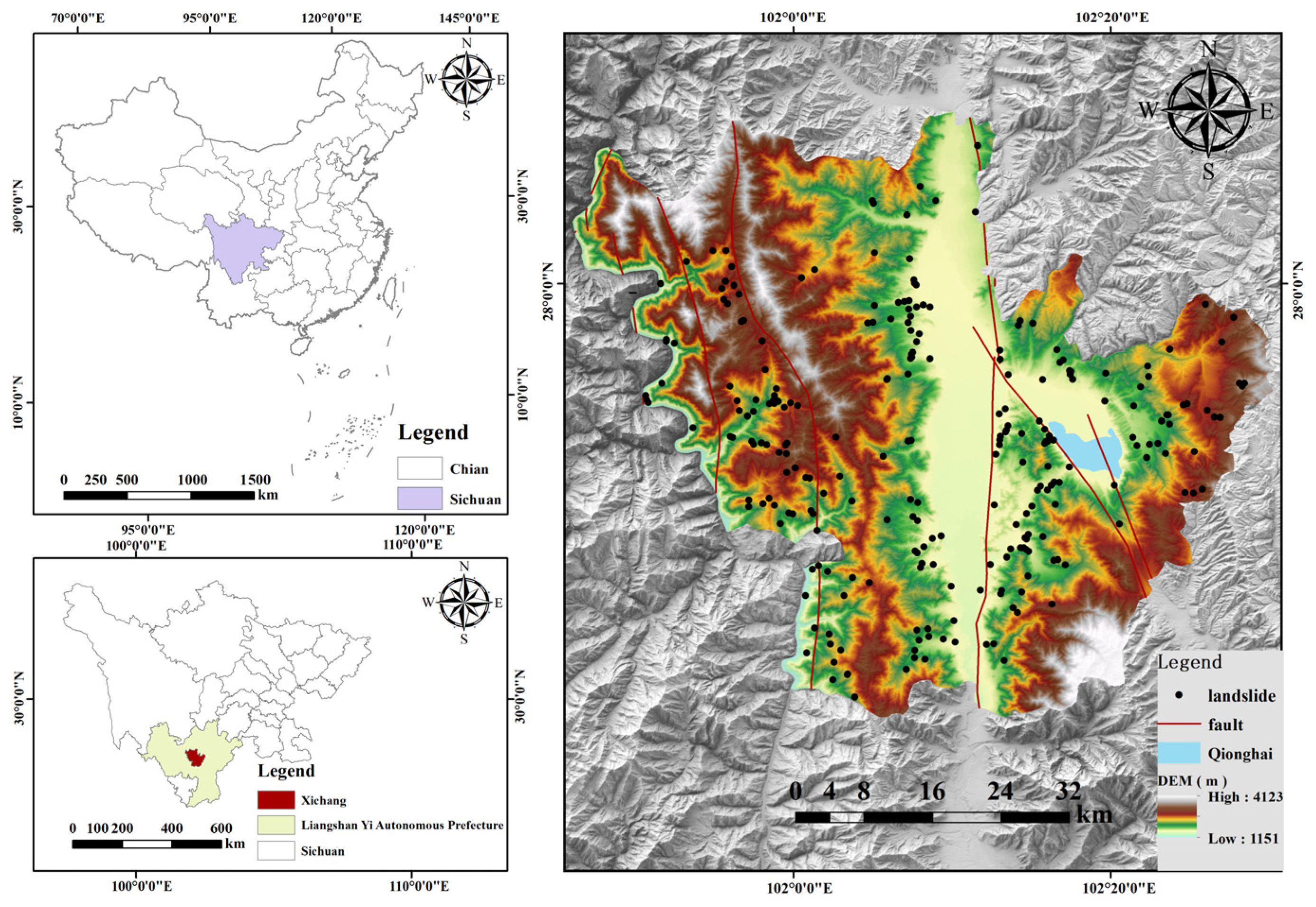
Situated in the southwest region of Sichuan Province, Xichang City spans a total area of approximately 2889.8 km², measuring approximately 20 km from north to south and 43 km from east to west. Its coordinates are longitude 101°46′ E to 102°25′ E and latitude 27°32′ N to 28°10′ N. The Zhongshan Mountains, located on both the east and west banks of the Anning River, dominate the landscape, and the city itself is situated at an elevation of more than 1500 m. The Yak Mountains, which form the watershed between the Anning and Yalong Rivers, are located in the west and span the entire region from north to south. The east side of the Anning River is part of the Luzhun Mountain Range, with the main ridge line located in Xide County in the north and the demarcation line between Xichang and Pugue in the south. The Yak Mountains contain numerous peaks that rise to elevations of over 3500 m, and these peaks gradually descend towards the south. There are many geological hazards in the region, but mudslides and landslides are the most common. Of all geological hazards in the city, 265 incidents account for 50.1% of the total. Figure 1 shows the geographic location of the study area.

3. Data Sources and Research Methods

3.1. Data Sources

Landslide distribution data with a resolution of 5 m were provided by the Geological Survey Bureau of Xichang City, Sichuan Province. A digital elevation model with a resolution of 12.5 m was provided by the Sichuan Provincial Bureau of Surveying, Mapping and Geoinformation for extracting hydrological data, such as topographic humidity indices, and recording topographic and geomorphological details, such as elevation, slope, and curvature. The road and river data of Xichang City were obtained from GF1 high-resolution remote sensing images. Land use type vector data were extracted from the Chinese annual land cover dataset with a resolution of 30 m using GIS tools. The normalized vegetation index (NDVI) was calculated using Landsat8 OL1 near- and far-infrared bands at 30 m resolution in May 2024 when the vegetation in the study area was at its densest, and the images can be downloaded from the US Geological Survey (https://earthexplorer.usgs.gov/, accessed on 18 February 2024). Fracture zone and stratigraphic rock data of the study area were obtained from the Centre for Resource and Environmental Science and Data of the Chinese Academy of Sciences (http://www.resdc.cn/, accessed on 16 May 2023), and the distance to the fracture zone and stratigraphic rock data were obtained by coordinate conversion. The extracted data were resampled using ArcGIS resampling at a resolution of 12.5 m using the same geospatial attributes. The data are presented in

Table 1. Source of data for Xichang landslide vulnerability assessment.

No.	Data	Scale
1	High-precision remote sensing image of GF1	1 m
2	Xichang County digital elevation model	12.5 m
3	Basic geological data of Wenchuan County	5 m × 5 m
4	Peak acceleration distribution map of Xichang County	5 m × 5 m
5	Annual land cover dataset for China, 1985–2022	30 m × 30 m
6	The Landsat 8 OLI image on 16 May 2024	30 m × 30 m
7	Landslide distribution data for Xichang	\

.

3.2. Research Methods

3.2.1. Integrated Learning Principles

Several base learners are used in integration learning, and their results are combined using an integration strategy for tasks involving regression or classification. The generalization performance of integrated learning is better than that of a single learner. Generally, there are two types of integrated learning: parallel methods, where there are no strong dependencies between base learners, and serial sequence methods, where there are strong dependencies between base learners. Boosting and Bagging are representatives in that order [29]. Additionally, the complexity of the overall model can be controlled by adjusting the model’s hyperparameters, such as the tree’s depth, the number of leaf nodes, and so forth, to limit the complexity of each base model. This helps address the issue of boost and bagging methods, which increase model complexity and consume large amounts of computational resources. This can keep prediction accuracy high while lowering the computational load. When working with large-scale data, XGBoost and LightGBM introduce more sophisticated techniques like tree weighting, column sampling, and histogram-based splitting, which make them more effective and computationally faster than other integrated learning algorithms like AdaBoost and regular gradient boosting. Furthermore, compared to the standard grow-by-layer approach, LightGBM’s leaf growth strategy is more flexible when dealing with large datasets and unbalanced data [30,31]. Thus, the RF algorithm based on bagging theory and the XGBoost and LightGBM algorithms based on boosting theory are used in this paper for modelling purposes, and the result is a landslide susceptibility prediction model with improved generalization performance.

3.2.2. Random Forest (RF)

An integrated learning algorithm called random forest (RF) builds several decision trees and combines their predictions to increase overall prediction accuracy. A decision tree is built for each training set using a random subset of features that were randomly selected from the original dataset. This process helps minimize overfitting by selecting a subset at random from the available features during the construction of each decision tree. The training set is used to train each decision tree until the stopping condition is met. Voting or averaging is used to determine the classification or regression results of the final predicted values when predictions are made for new data. The training results of each decision tree are combined based on the bagging integration concept [32]. The schematic diagram of the random forest model is shown in Figure 2.

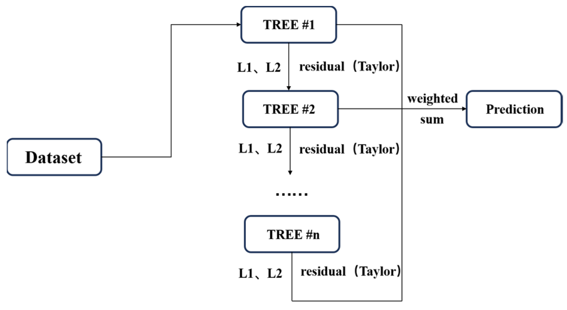
3.2.3. Extreme Gradient Boosting Tree (XGBoost)

The Extreme Gradient Boosting Tree (XGBoost) is an improved optimization algorithm based on the GBDT. Like traditional GBDT, both are serial serialization algorithms based on boosting integration that focus on the residuals between the prediction result of the previous decision tree and the measured value. The training stops after reaching a set value or number of iterations to fit the residuals and approximate the measured value. The weighted sum of the prediction results from each tree is the final prediction of this sample in the whole integrated model. The difference is that when solving the loss function, XGBoost uses Taylor’s second-order expansion to simplify the computation and introduces regular terms such as L1 and L2 in the objective value to control the complexity of the model and prevent overfitting. Compared with the traditional GBDT algorithm, the XGBoost algorithm has a higher computational efficiency and the ability to prevent overfitting [33]. The schematic diagram of the XGBoost model is shown in Figure 3

3.2.4. Light Gradient Boosting Machine (LightGBM)

Similar to XGBoost, Light Gradient Boosting Machine (LightGBM) is an enhanced optimization algorithm built on the GBDT algorithm. The distinction is that LightGBM uses a histogram algorithm to discretize the continuous feature values into multiple bins. Based on the bins where the features are located, it accumulates the gradient, counts the number of features, and finally iterates through all features and data to find the optimal splitting point. This solves the problem of an excessive number of splitting points, improves the training efficiency of the decision tree, and reduces memory consumption [33]. Additionally, the leaf growth (leaf-wise) algorithm with depth restriction, which is based on the histogram algorithm, is used to split only the leaf node with the largest splitting gain each time, thereby reducing the complexity of the model and simultaneously improving the overfitting resistance [34]. The schematic diagram of the LightGBM model is shown in Figure 4.

3.2.5. Bayesian Optimization Algorithm (BO)

The global behavior of the objective function is first established a priori using the Bayesian optimization algorithm (BO), which then updates this prior knowledge by observing the output of the objective function at various input points to form a posterior distribution [23]. The next sampling point is chosen based on the a posteriori distribution, and this selection considers both globally unexplored regions and previously observed optimal values. This allows for a more effective search during the hyperparameter tuning. The formula is as follows:

$${\rm P}\left(f|D_{1:t}\right)={\displaystyle \frac{P\left(D_{1:t}|f\right)P\left(f\right)}{P\left(D\right)}}$$

(1)

where: f denotes the defined objective function; $D_{1:t}$ = $\{\left(x_1,y_1\right),\left(x_2,y_2\right),\dots ,\left(x_t,y_t\right)\}$ denotes the set of observations, and $x_t$ denotes the decision vector; $y_t=f\left(x_t\right)+{\epsilon }_t$ denotes the observation value, and ${\epsilon }_t$ denotes the observation error; ${\rm P}\left(f|D_{1:t}\right)$ denotes the likelihood distribution of $f$; $P\left(f\right)$ denotes the prior probability distribution, which is an assumption based on the black-box objective function; $P\left(D_{1:t}\right)$ denotes the marginal likelihood distribution of $f$; $P\left(D\right)$ acts as a coefficient; and ${\rm P}\left(f|D_{1:t}\right)$ denotes the posterior probability distribution of $f$.

3.2.6. Performance Evaluation of the Models

1.

Accuracy, Precision, Recall, and F1 score

An essential part of the landslide susceptibility assessment process is the model validation and performance assessment. Typically, the performance of a binary classification model is assessed using a confusion matrix. Four parameters make up the confusion matrix. True positive (TP) is the number of landslide points predicted by the model that are actual landslide points. False negative (FN) is the number of non-landslide points predicted by the model that are landslide points. The number of landslide points that the model predicts, but which are in fact non-landslide points, is known as false positive (FP). The number of non-landslide points that the model predicts that are in fact non-landslide points is known as true negative (TN). Based on this, the performance of each model was assessed using four statistical metrics: accuracy, precision, recall, and F1 score [35].

Table 2. Characteristics of statistical indices described using a confusion matrix.

Index	Formulas	Description
Accuracy	${\displaystyle \frac{TP+TN}{TP+FP+TN+FN}}$	Calculates the percentage of samples that were accurately predicted.
Precision	${\displaystyle \frac{TP}{TP+FP}}$	Calculates the TP sample percentage in each predicted positive sample.
Recall	${\displaystyle \frac{TP}{TP+FN}}$	Calculates the TP sample’s percentage in each true positive sample.
F1	${\displaystyle \frac{2\times Precision\times Recall}{Precision+Recall}}$	Represents the accuracy and recall harmonic mean, with a range of values from −1 to 1.

displays descriptions of each index.

2.

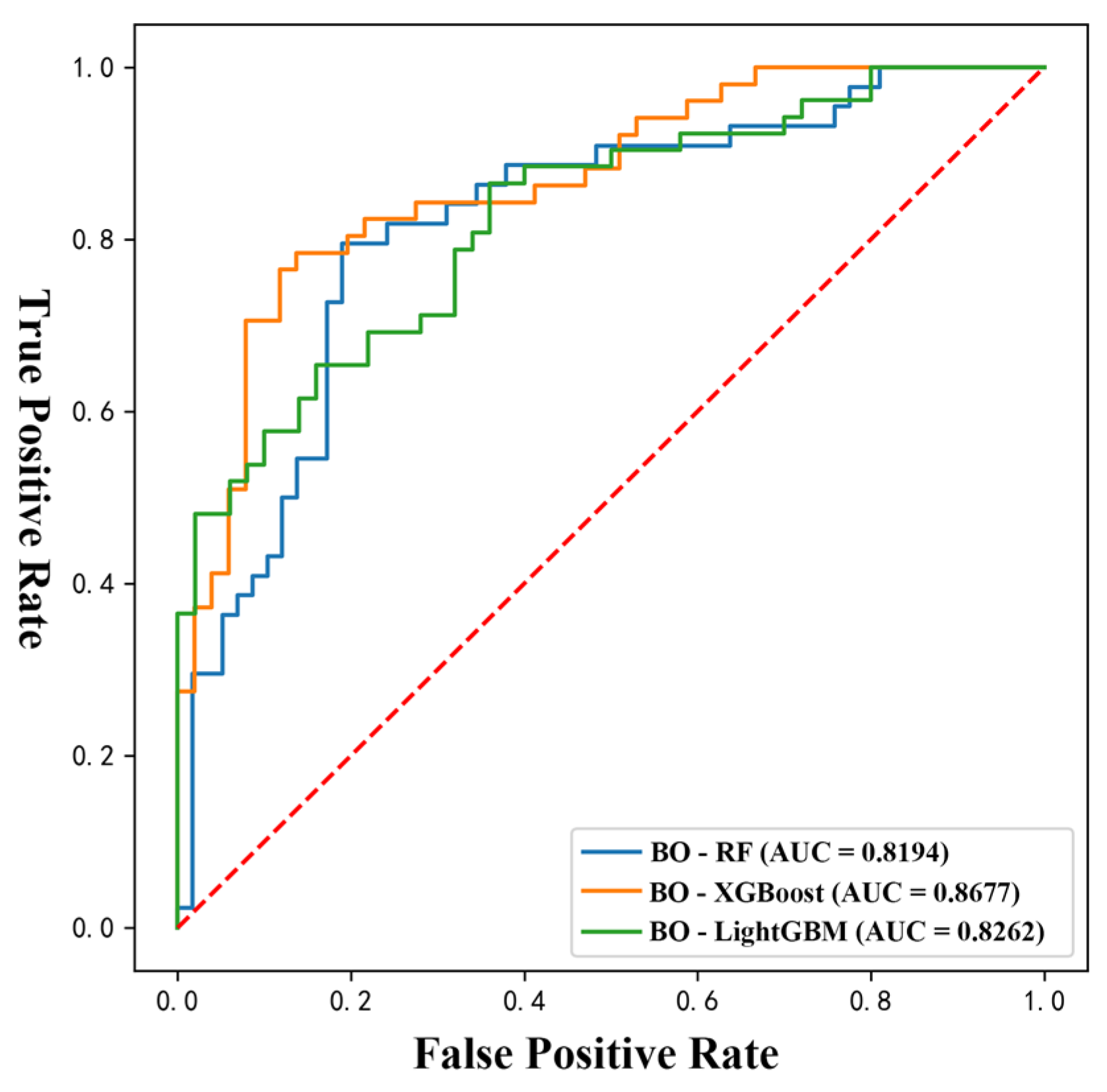
ROC curve and AUC value

The true positive rate (TPR) on the vertical axis and the false positive rate (FPR) on the horizontal axis represent the true positive rate (ROC) curve, which illustrates the performance of the model at various classification thresholds. Whereas FPR shows the percentage of samples that are incorrectly predicted as negative cases, TPR shows the percentage of samples that are accurately predicted as positive cases. The performance of the model is indicated by how close the ROC curve is to the upper left corner. The area under the ROC curve, which offers a thorough evaluation of the model performance, is known as the area under the curve (AUC) value [36]. The model’s predictive performance is comparable to random guessing when the AUC value is 0 (no discrimination between positive and negative cases) and 1 (perfect discrimination). The model performs better; therefore, the AUC value is closer to 1.

4. Results

4.1. Selection and Identification of Evaluation Indicators

After sorting and screening the Xichang City landslide disaster site data, 265 landslide sites were selected as statistical indicators for the analysis. Based on the ground survey data and the historical incidence of geological disasters, 13 influencing factors were chosen as indicators to assess the influence of landslide disaster susceptibility in the study area. An explanation for the selection of influencing factors is provided in

Table 3. Rationale for selecting evaluation factors.

Factors	Fundamental Principle
Normalized difference vegetation index (NDVI)	The NDVI is a crucial metric for measuring the amount and cover of vegetation and helps to lower the frequency of landslides. Xichang City’s Landsat 8 image data were processed to create an NDVI.
Topographic wetness index (TWI)	Considering factors like surface runoff patterns, buried groundwater depth, and topographic relief, the topographic wetness index (TWI) is a helpful tool for determining an area’s topographic wetness. The hydrological processing of Xichang City’s 12.5 m DEM data was utilized to determine its TWI.
Stream power index (SPI)	Using the stream power index (SPI), one can measure the impact of water flow intensity on landslide stability by looking at how it appears on the surface of the landslide body. Hydrological processing of Xichang City’s 12.5 m DEM data produced the SPI.
Peak ground acceleration (PGA)	Peak seismic acceleration is one of the most important features for determining the intensity of an earthquake.
Distance from the road	Landslides generally pose a greater risk to roads when they occur near to them than when they occur far from them. Xichang City traffic road vector data’s multi-ring buffer was analyzed to determine the distribution of landslides with respect to road distance.
Distance from water system	Because of their complex geological structures and steeper topography, areas near water systems are more prone to landslides. The distribution of the distance between the disaster sites and the water system was found by analyzing the vector data of the water system in the multi-ring buffer zone of Xichang City.
Distance from faults	Landslides are more common in areas close to faults. The fault vector data in the multi-ring buffer zone of Xichang City was analyzed in order to determine the distribution of hazard points with respect to the distance from faults.
Slope	Slope is a significant contributing factor to slope instability and influences the direction of water flow and soil development. To ascertain the distribution of slope and disaster points, the Xichang City 12.5 m DEM data were processed.
Relief intensity	The height differential between the surface’s highest and lowest points divided by the horizontal distance represents the degree of topographic relief. From the focal statistics of the 12.5 m DEM data in Xichang City, the distribution of disaster points and their relative height difference was obtained.
Aspect	Landslides typically occur more frequently on sunny, windward slopes than on leeward or backward slopes. From the slope orientation analysis of its 12.5 m DEM data, the distribution of hazard points on Xichang City’s slopes was determined.
Curvature	Landslide occurrence and development are significantly impacted by the degree of terrain curvature, which can be reflected in curvature. From the focal statistics of its 12.5 m DEM data, the curvature of Xichang City is obtained.
Lithology	Lithology is a significant source of material detriment to landslides. Landslides can originate and progress in different ways depending on the lithological strata beneath them. Xichang City’s lithology and disaster points are distributed based on cropping in accordance with the current geological map.
Land use type	Apart from soil moisture and surface runoff, land use type also indirectly influences the evolution of landslides.

. Using ArcGIS 10.8 software, the DEM data with a resolution of 12.5 m × 12.5 m were transformed to display the relationship between each graded influence factor and hazard, as shown in Figure 5.

Table 4. Impact factor and landslide point classification statistics table for Xichang City.

Name of Indicator	Grading	Area/(km2)	Number of Disaster Points/(pcs)	Percentage of Region (%)	Density of Disaster Sites/(km2)
NDVI	0.200	426.439	49	14.76	0.017
	0.400	784.165	135	27.14	0.047
	0.600	559.252	56	19.35	0.019
	0.800	476.220	15	16.48	0.005
	1.000	643.724	10	22.28	0.003
TWI	0.200	2225.405	214	77.01	0.074
	0.400	470.698	47	16.29	0.016
	0.600	158.892	3	5.50	0.001
	0.800	31.943	1	1.11	0.000
	1.000	1.962	0	0.07	0.000
PGA	<0.2	390.072	39	13.50	0.013
	0.2–0.4	1007.420	105	34.86	0.036
	>0.4	1491.409	121	51.61	0.042
SPI	0.200	140.927	1	4.88	0.000
	0.400	439.454	39	15.21	0.013
	0.600	2171.420	215	75.14	0.074
	0.800	132.601	10	4.59	0.003
	1.000	4.498	0	0.16	0.000
Distance from road	<100	236.905	35	8.20	0.012
	100–200	182.917	21	6.33	0.007
	200–300	155.496	20	5.38	0.007
	300–500	257.148	31	8.90	0.011
	>500	2056.433	158	71.16	0.055
Distance from fault	<1000	452.449	42	15.66	0.015
	1000–2000	410.124	20	14.19	0.007
	2000–3000	673.569	76	23.31	0.026
	3000–5000	474.898	42	16.43	0.015
	>5000	877.860	85	30.38	0.029
Distance from river	200.000	910.283	92	31.50	0.032
	200–400	649.345	65	22.47	0.022
	400–600	443.853	49	15.36	0.017
	600–800	298.829	29	10.34	0.010
	>800	586.590	30	20.30	0.010
Slope	<10	693.657	42	24.00	0.015
	10–20	592.384	96	20.50	0.033
	20–30	813.586	85	28.15	0.029
	30–40	579.051	36	20.04	0.012
	>40	211.122	6	7.31	0.002
Relief intensity	<10	1144.384	115	39.60	0.040
	10–20	1104.339	113	38.22	0.039
	20–30	492.241	33	17.03	0.011
	30–40	108.288	4	3.75	0.001
	>40	39.647	0	1.37	0.000
Aspect	North	459.655	31	15.91	0.011
	Northeast	293.037	24	10.14	0.008
	East	324.511	22	11.23	0.008
	Southeast	345.276	24	11.95	0.008
	South	392.865	39	13.59	0.013
	Southwest	392.814	40	13.59	0.014
	West	358.308	52	12.40	0.018
	Northwest	322.434	33	11.16	0.011
Curvature	<−2.56	144.535	10	5.00	0.003
	−2.56–−0.64	978.953	100	33.88	0.035
	−0.64–0.64	1108.982	102	38.38	0.035
	0.64–2.66	589.239	51	20.39	0.018
	>2.66	67.192	2	2.33	0.001
Land use type	Cultivated	722.412	96	25.00	0.033
	Forest	1584.540	103	54.83	0.036
	Grass	300.467	45	10.40	0.016
	Brushland	18.887	2	0.65	0.001
	Wetland	1.132	1	0.04	0.000
	Tundra	63.069	3	2.18	0.001
	Manmade	164.110	0	5.68	0.000
	Bare soil	34.035	10	1.18	0.003
	Glacier	0.248	5	0.01	0.002
Lithology	Basalt	1290.207	122	44.65	0.042
	Shale	184.387	43	6.38	0.015
	Sandstone	795.655	78	27.53	0.027
	Limestone	341.046	9	11.80	0.003
	Slate	141.239	0	4.89	0.000
	Streams	11.607	0	0.40	0.000
	Gravel	97.829	13	3.39	0.004
	Lochs	26.931	0	0.93	0.000

presents comprehensive ranked statistical data on risk locations and influencing variables.

4.2. Correlation Analysis of the Factors

Correlation analyses were carried out on the 13 factors that were initially chosen to determine which evaluation factors had the best predictive power and to increase the precision of the model prediction. The matrix of correlation coefficients between the 13 influencing factors can be obtained and visualized to create Figure 6 using the Correlation Plot plug-in of the Origin 2022 plotting software. In the graph, negative correlations are displayed in blue, and positive correlations are shown in red. The size of the image directly affects the magnitude of the correlation coefficient. The figure illustrates that the correlation coefficient between the slope and terrain relief is 0.91, signifying a large factor interaction. Consequently, the evaluation factor for terrain relief is excluded. The remaining factors have correlation coefficients less than 0.38, indicating weaker factor interactions and more reasonable evaluation factors.

4.3. Multi-Collinearity Test

The tolerance (TOL) and variance inflation factor (VIF) values of the landslide susceptibility evaluation factors were calculated using analysis of covariance (ANCOVA) and SPSS 27.0.1 software, as indicated in

Table 5. Collinearity diagnostic results of influence factors.

Factors	TOL	VIF
NDVI	0.719	1.392
TWI	0.671	1.490
SPI	0.734	1.363
PGA	0.845	1.184
Distance from road	0.868	1.152
Distance from water	0.905	1.105
Distance from fault	0.802	1.247
Slope	0.493	2.027
Aspect	0.952	1.051
Curvature	0.976	1.025
Lithology	0.881	1.135
Land use type	0.839	1.192

. The VIF value is less than 2.5, which is significantly lower than the threshold values of 5 or 10, indicating that there is no multicollinearity between the selected factors. This again confirms the rationality of the evaluation factors. The TOL values of the evaluation factors are all greater than 0.4, which is significantly higher than the threshold value of 0.1.

4.4. Evaluation of Susceptibility and Accuracy Analysis

4.4.1. Bayesian Hyperparametric Optimization Analysis

In Xichang City, there have been 265 landslides in total. Using the ArcGIS random generation tool, 265 non-landslide points were created in the non-landslide areas so that the number of positive samples (landslide points) equaled the number of negative samples (non-landslide points) in order to create the dataset for the model. Within the dataset, landslide points were assigned a target value of 1, while non-landslide points were assigned a target value of 0. To increase the model’s validation accuracy and training effect, the entire dataset was split into a 20% test set and an 80% training set. The model in this paper is not normalized or standardized on the input features because landslides are classified as classification problems, and the integrated learning algorithm with a decision tree-based learner is insensitive to feature scaling. Instead, the categorical values of the 12 evaluation factors are extracted into the dataset using the ArcGIS reclassification and multi-value extraction tools. These values were then fed into the machine learning package through Scikit-learn to build the susceptibility model based on the three integrated algorithms: RF, XGBoost, and LightGBM.

In this paper, a Bayesian optimization algorithm is chosen to optimize the established models by searching in the selected hyperparameter space to find the best combination of hyperparameters. For optimizing the XGBoost, RF, and LightGBM models, a threshold of 200 iterations is set. In each iteration, the dataset is divided into 10 subsets, of which 9 are used to train the model and 1 is used to validate the model [37]. Through this 10-fold cross-validation method, the average of the model accuracy is calculated as the performance assessment metric of the model. Finally, the optimal hyperparameters of the three models were obtained using Bayesian algorithm optimization as shown in

Table 6. Hyperparametric optimal combinations of XGBoost, LightGBM, and random forest.

Model	Parameterization	Definition	Search Scope	Optimum Value
XGBoost	n_estimators	Number of decision trees	(100, 1500)	1288
	random_state	Random tree seed	(10, 50)	25
	max_depth	Maximum depth of the tree	(3, 10)	8
	min_child_weight	Decide the minimum leaf node sample weights	(1, 10)	3
	Learning_rate	The step size when iterating the decision tree	(0.01, 0.2)	0.06
	Gamma	Minimum loss function drop value	(0, 1)	0.91
	Subsample	Random sampling with put-back	(0.5, 1)	0.98
	colsample_bytree	Control the percentage of columns sampled randomly in each tree	(0.5, 1)	0.92
LightGBM	n_estimators	Number of decision trees	(100, 1500)	1304
	max_depth	Maximum depth of the tree	(3, 10)	3
	num_leaves	Specify the number of leaves	(3, 50)	15
	min_child_samples	Minimum number of leaf node samples	(3, 50)	21
	Subsample	Random sampling with put-back	(0.5, 1)	0.71
	colsample_bytree	Control the percentage of columns sampled randomly in each tree	(0.5, 1)	0.89
	learning_rate	The step size when iterating the decision tree	(0.01, 0.2)	0.06
RF	n_estimators	Number of decision trees	(100, 1500)	1273
	min_samples_split	Minimum number of samples required to perform a split	(3, 15)	5
	min_samples_leaf	Minimum number of samples for leaf nodes	(3, 15)	4
	max_features	Maximum number of features considered in constructing the decision tree	(0.1, 0.99)	0.5
	max_depth	Maximum depth of the tree	(3, 15)	6

. Figure 7 shows the iterative process of the Bayesian algorithm in optimizing these three models.

To verify the efficacy of Bayesian hyperparameter optimization, three models with default parameters were also developed for comparison in the study.

Table 7. The accuracy of the three models is compared before and after Bayesian optimization.

Model	Unhyperparameterized Optimization	After Hyperparameter Optimization	Average Accuracy Improvement (%)
XGBoost	0.746	0.794	6.4
LightGBM	0.701	0.735	4.9
RF	0.653	0.692	6.0

As can be seen from the table, the average accuracy of XGBoost, LightGBM, and RF models were improved by 5.4%, 3.4%, and 6.0%, respectively. The prediction accuracy of the models after Bayesian optimization is significantly improved.

presents the findings from a comparison of the mean precision of the 10-fold cross-validation conducted prior to and following Bayesian hyperparameter optimization.

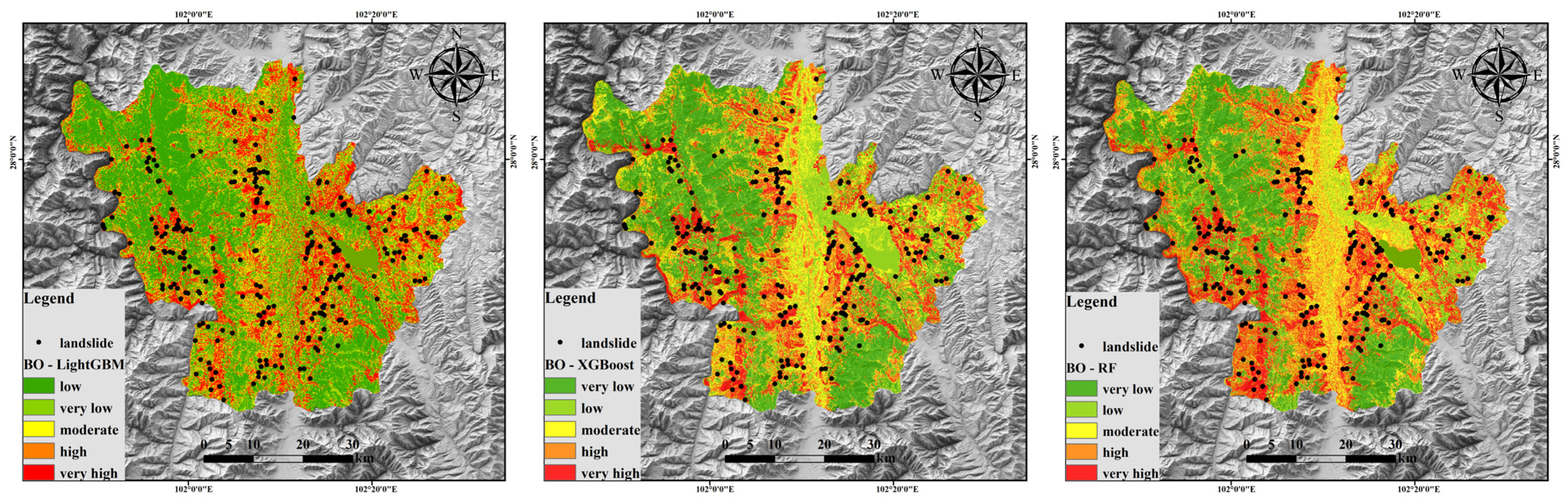
4.4.2. Landslides Based on BO-RF, BO-XGBoost, and BO-LightGBM Model Vulnerability Mapping

The study area consists of 381,275 raster cells, which are converted to point elements in ArcGIS 10.8. The trained integrated learning model is used to calculate the landslide susceptibility index for each point, and the classification values are extracted by the selected 12 evaluation feature factors. Using the natural breakpoint method, the landslide hazard risk was categorized into five classes: very high, high, moderate, low, and very low susceptibility zones. Lastly, the landslide hazard susceptibility zoning map (Figure 8) was created using the BO-RF, BO-XGBoost, and BO-LightGBM models. The distribution number of landslide sites for each grade and the results of the susceptibility zoning were counted (

Table 8. BO-XGBoost, BO-LightGBM, and BO-RF susceptibility statistic table.

Model	Statistical Data	Very Low	Low	Moderate	High	Very High
BO-LightGBM	Area (km2)	1293.94	654.74	441.44	274.19	225.49
	Number of disaster points	24	43	55	65	78
	Area ratio	44.78	22.66	15.28	9.49	7.80
	Disaster points density (ind/km2)	0.019	0.066	0.125	0.237	0.346
BO-XGBoost	Area (km2)	1099.91	664.38	569.39	381.31	174.82
	Number of disaster points	19	31	71	73	71
	Area ratio	38.06	22.99	19.70	13.20	6.05
	Disaster points density (ind/km2)	0.017	0.047	0.125	0.191	0.406
BO-RF	Area (km2)	971.52	797.08	572.52	353.32	195.36
	Number of disaster points	27	40	72	73	53
	Area ratio	33.62	27.58	19.81	12.23	6.3376
	Disaster points density (ind/km2)	0.028	0.050	0.126	0.207	0.271

). The areas of very high susceptibility zones for the BO-XGBoost, BO-LightGBM, and BO-RF models were 174.82 km², 225.49 km², and 195.36 km², respectively; the density of the hazard sites in the very high susceptibility zones was 0.406/km², 0.346/km², and 0.271/km², respectively. The susceptibility statistics for the BO-XGBoost, BO-LightGBM, and BO-RF model are shown in Figure 9. The three models successfully predicted the likelihood of landslides in Xichang City in accordance with the actual situation, as evidenced by the fact that the density of disaster sites increased with the degree of susceptibility. The hazard point density of the BO-XGBoost model is higher in the very high susceptibility area and lower in the very low susceptibility area when compared to the BO-LightGBM and BO-RF models in different susceptibility areas. Thus, it can be said that in Xichang City, the BO-XGBoost model is better suited for use as a landslide susceptibility assessment model.

4.4.3. Evaluation of Model Accuracy

By importing the metrics library in sklearn in Python 3.10, the accuracy, precision, recall, F1 score, ROC curve, and AUC values of the BO-XGBoost, BO-LightGBM, and BO-RF models were determined, as indicated in

Table 9. Accuracy of each integrated learning model.

Metrics	BO-XGBoost	BO-LightGBM	BO-RF
Accuracy	0.794	0.706	0.716
Precision	0.788	0.720	0.619
Recall	0.804	0.692	0.886
F1 score	0.796	0.706	0.729

, and visualized in Matplotlib to produce Figure 10 and Figure 11.

Table 9 and Figure 10 demonstrate that, in terms of performance metrics, the integrated learning models of BO-XGBoost and BO-LightGBM based on boosting are more stable than BO-RF based on bagging. Additionally, the performance metrics of the BO-XGBoost model are higher than those of BO-LightGBM overall, suggesting that the XGBoost model outperforms the LightGBM model with higher prediction accuracy and better generalization ability in finite classification problems.

Figure 11 shows that, following Bayesian parameter optimization, the BO-XGBoost model is closer to the upper left corner, with an AUC value of 0.8677, which is higher than that of the BO-RF and BO-LightGBM models. When compared to RF, XGBoost and LightGBM enhance the model’s loss function and introduce a regular term to account for complexity, which enhances the model to some degree. LightGBM is derived from XGBoost, which maximizes the model’s training speed; however, XGBoost exhibits superior generalization capabilities and high reliability in susceptibility zoning.

4.5. Importance of Evaluation Factors

This study performed an importance analysis of 12 landslide evaluation feature factors based on the BO-XGBoost model to determine the most significant features for the prediction results. Weight, gain, and cover are the three types of metrics that the XGBoost model offers to determine the feature importance. The weight of a feature indicates how many times it has been used across all trees. Gain indicates the average gain of a feature to the prediction result in all trees. This parameter represents the importance of the feature because a feature contributes more to the final prediction result if it is used in more trees. Cover indicates the average coverage of samples by a feature across all trees. This parameter indicates the feature’s ability to split at each node since a feature that splits more at each node contributes more to the final prediction result. This parameter indicates how well a feature covers the model since a feature affects more samples overall, which increases its contribution to the final prediction. Figure 12 displays the findings regarding the significance of the influencing factors.

5. Discussion

Despite substantial research dedicated to landslide susceptibility assessment, many gaps and deficiencies remain. First, most existing studies employ a single machine learning model, which struggles to capture the landslide-triggering mechanisms under complex geological conditions [38,39]. Additionally, there is limited research on parameter optimization in landslide susceptibility assessments, with traditional optimization algorithms being inefficient and prone to local optima [22,40,41,42]. Addressing these issues, this paper presents a context focusing on the landslide risk in Xichang under potential future strong earthquakes [43], introducing ensemble learning algorithms and Bayesian optimization to enhance model generalization and prediction accuracy.

From Figure 12, it is evident that the significance of the influencing factors derived from the three indicators is largely consistent. The four most important influencing factors are NDVI, slope, distance to rivers, and distance to faults. NDVI is the most significant influencing factor in Xichang, with areas of low vegetation coverage accounting for 41.89% of the total area. Exposed ground or sparsely vegetated soil creates space for landslides to develop, potentially increasing regional landslide activity. Xichang is located in the articulated section of the Xianshuihe Fault system, situated between the Anning River and Zemu River faults. The activity, direction, and dip of these faults directly impact landslide formation. Most landslide disasters in Xichang occur in areas with slopes between 10° and 30°, where the terrain is relatively steep and variable, significantly increasing the risk of landslides. As part of the Anning River Basin, Xichang has many tributaries on both sides of the main rivers. River erosion causes steep banks, which is where most landslides in the region occur. The significance of evaluation factors derived from the BO-XGBoost model aligns with the actual conditions of the study area and the results of earlier research [44,45,46,47], providing substantial evidence for the validity of the study’s findings.

The boosting model employed in this work has major advantages over other studies. For instance, while many researchers have employed a variety of machine learning techniques to assess the susceptibility of landslides and have produced some results, they have typically been unable to resolve the issue of model parameter optimization [48,49,50]. In this study, Bayesian optimization effectively solves this issue, enhancing the model’s accuracy and dependability. More specifically, by enhancing the loss function and adding regularization terms, BO-XGBoost and BO-LightGBM both increase training speed and successfully avoid overfitting. In contrast, the boosting algorithm outperforms the bagging algorithm in handling complex geological conditions, even though it integrates multiple decision trees to increase the stability of the model. In this study, the BO-RF model outperforms the BO-XGBoost model in terms of accuracy, precision, and F1 score, but it has a higher recall. Since landslide-prone areas are more likely to be identified as positive classes when using RF, the recall rate is higher but the precision rate is lower as a result of the rise in false positives. Furthermore, the RF model may be more sensitive to the minority class (landslide events) if there are fewer positive class samples in the landslide dataset. This would result in a higher recall.

Although this study has achieved significant results, there are certain limitations. First, the geological environment of the study area is complex and variable, with different regions potentially having distinct landslide-triggering mechanisms, which limits the model’s applicability to other areas. Additionally, landslide susceptibility is typically influenced by multiple environmental factors. If these variables are not adequately considered, the model may struggle to accurately capture the complex mechanisms underlying landslide occurrences. For instance, over time, climate change could alter rainfall patterns, thereby affecting the frequency and distribution of landslides. If the model does not dynamically update to account for these changing factors, it may either overestimate or underestimate future landslide susceptibility.

This study considered only 12 feature factors; future research could incorporate a broader range of geological and meteorological data to improve the model’s accuracy. For example, future studies should integrate real-time monitoring data, such as rainfall and seismic activity, particularly in conjunction with InSAR technology, to enhance the predictive capability and timeliness of the model. Furthermore, the application of ensemble learning and Bayesian optimization algorithms in landslide susceptibility assessment should be further explored, particularly in optimizing model parameters under varying geological conditions. Lastly, the reliability and applicability of the model should be further validated using geological surveys and field verification.

6. Conclusions

The number of landslides within each evaluation factor’s grading range was counted. The NDVI was 0.2–0.4, TWI was less than 0.2, PGA was greater than 0.4, and SPI was 0.4–0.6. The area with basalt lithology and located 500 m from the road had the highest number of landslides.

The accuracy of the BO-XGBoost, BO-LightGBM, and BO-RF models increased by 6%, 4%, and 9%, respectively, after 10-fold cross-validation and Bayesian optimization of hyperparameters. The BO-XGBoost model performed the best, with an AUC value of 0.8677 and higher accuracy, F1-score, generalization ability, and fit than the other two models.

Weight, gain, and cover indicators were used to conduct an importance analysis of the 12 landslide evaluation factors on the BO-XGBoost-based model. The findings indicated that the most significant characteristic factors to be considered when developing disaster prevention and mitigation related measures were NDVI, distance from the fault, slope, and distance from the river.

References

- Fan, X.; Gong, X.; Cai, F.; Huang, D. Dynamic Changes of Locking and Slip Distribution in the Anninghe-Zemuhe Fault Zone. Chin. J. Geophys. 2023, 43, 914–918. [Google Scholar]
- Ren, J.; Li, P. Characteristics of surface rupture of the Xichang 1850 earthquake, Sichuan, China. Seismol. Geol. 1993, 2, 97–106+193–194. [Google Scholar]
- Qin, S.; Li, P.; Xue, L.; Li, G.; Abbas, F. Definition of strong-seismic gestation cycles in selected seismic zones in southwestern China. Prog. Geophys. 2014, 29, 1526–1540. [Google Scholar]
- Xu, W.; Zheng, X.; Ou, W.; Tie, Y. Characteristics of losses of geological disasters and major disaster types in Liangshan Prefecture, Sichuan province. Chin. J. Geol. Hazard. Control 2023, 35, 1–12. [Google Scholar]
- Wang, H.J.; Zhang, L.M.; Luo, H.Y.; He, J.; Cheung, R.W.M. AI-powered landslide susceptibility assessment in Hong Kong. Eng. Geol. 2021, 288, 106103. [Google Scholar] [CrossRef]
- Wang, Y.; Fang, Z.C.; Hong, H.Y. Comparison of convolutional neural networks for landslide susceptibility mapping in Yanshan County, China. Sci. Total Environ. 2019, 666, 975–993. [Google Scholar] [CrossRef]
- Phuong, T.T.N.; Panahi, M.; Khosravi, K.; Ghorbanzadeh, O.; Kariminejad, N.; Cerda, A.; Lee, S. Evaluation of deep learning algorithms for national scale landslide susceptibility mapping of Iran. Geosci. Front. 2021, 12, 505–519. [Google Scholar]
- Jiang, W.; Li, Y.; Yang, X.; Deng, X.; Abbas, F. Study on Landslide Susceptibility in Nujiang Prefecture Based on Slope Unit. J. Soil. Water Conserv. 2023, 37, 160–167. [Google Scholar]
- Li, Z.; Wang, T.; Zhou, Y.; Liu, J.; Abbas, F. Landslide Susceptibility Assessment Based on Information Value Model Logistic Regression Model and Their Integrated Model: A Case in Shatang River Basin, Qinghai Province. Geoscience 2019, 33, 235–245. [Google Scholar]
- Zhang, Z.; Deng, M.; Xu, S.; Zhang, Y.; Abbas, F. Comparison of landslide susceptibility assessment models in Zhenkang County, Yunnan Province, China. Chin. J. Rock. Mech. Eng. 2022, 41, 157–171. [Google Scholar]
- Zhang, X.; Jiang, Y.; Wang, Y.; Qi, Z.; Abbas, F. Evaluation of landslide susceptibility based on multi-objective optimization method. J. Soil. Water Conserv. 2024, 38, 104–112. [Google Scholar]
- Wang, Q.; Xiong, J.; Cheng, W.; Cui, X.; Abbas, F. Landslide susceptibility mapping methods coupling with statistical methods, machine learning models and clustering algorithms. Int. J. Geogr. Inf. Sci. 2024, 26, 620–637. [Google Scholar]
- Huang, Y.; Zhao, L. Review on landslide susceptibility mapping using support vector machines. Catena 2018, 165, 520–529. [Google Scholar] [CrossRef]
- Huang, F.M.; Xiong, H.W.; Yao, C.; Catani, F.; Zhou, C.; Huang, J. Uncertainties of landslide susceptibility prediction considering different landslide types. J. Rock. Mech. Geotech. 2023, 15, 2954–2972. [Google Scholar] [CrossRef]
- Merghadi, A.; Yunus, A.P.; Dou, J.; Whiteley, J.; Binh, T.; Dieu, T.B.; Avtar, R.; Abderrahmane, B. Machine learning methods for landslide susceptibility studies: A comparative overview of algorithm performance. Earth-Sci. Rev. 2020, 207, 103225. [Google Scholar] [CrossRef]
- Sun, D.L.; Gu, Q.Y.; Wen, H.J.; Xu, J.H.; Zhang, Y.; Shi, S.; Xue, M.; Zhou, X. Assessment of landslide susceptibility along mountain highways based on different machine learning algorithms and mapping units by hybrid factors screening and sample optimization. Gondwana Res. 2023, 123, 89–106. [Google Scholar] [CrossRef]
- Yang, C.; Liu, L.L.; Huang, F.M.; Huang, L.; Wang, X. Machine learning-based landslide susceptibility assessment with optimized ratio of landslide to non-landslide samples. Gondwana Res. 2023, 123, 198–216. [Google Scholar] [CrossRef]
- Chen, Y.; Li, N.; Zhao, B.; Xing, F.; Xiang, H. Comparison of informative modelling and machine learning methods in landslide vulnerability evaluation—A case study of Wenchuan County, China. Geocarto Int. 2024, 39, 2361714. [Google Scholar] [CrossRef]
- Wu, Y.L.; Ke, Y.T.; Chen, Z.; Liang, S.Y.; Zhao, H.; Hong, H. Application of alternating decision tree with AdaBoost and bagging ensembles for landslide susceptibility mapping. Catena 2020, 187, 104396. [Google Scholar] [CrossRef]
- Zeng, T.R.; Wu, L.Y.; Peduto, D.; Glade, T.; Hayakawa, Y.S.; Yin, K. Ensemble learning framework for landslide susceptibility mapping: Different basic classifier and ensemble strategy. Geosci. Front. 2023, 14, 101645. [Google Scholar] [CrossRef]
- Dou, J.; Yunus, A.P.; Dieu, T.B.; Merghadi, A.; Sahana, M.; Zhu, Z.; Chen, C.; Han, Z.; Binh, T.P. Improved landslide assessment using support vector machine with bagging, boosting, and stacking ensemble machine learning framework in a mountainous watershed, Japan. Landslides 2020, 17, 641–658. [Google Scholar] [CrossRef]
- Kavzoglu, T.; Teke, A. Advanced hyperparameter optimization for improved spatial prediction of shallow landslides using extreme gradient boosting (XGBoost). Bull. Eng. Geol. Environ. 2022, 81, 201. [Google Scholar] [CrossRef]
- Sun, D.L.; Xu, J.H.; Wen, H.J.; Wang, D.Z. Assessment of landslide susceptibility mapping based on Bayesian hyperparameter optimization: A comparison between logistic regression and random forest. Eng. Geol. 2021, 281, 105972. [Google Scholar] [CrossRef]
- Xia, D.; Tang, H.M.; Sun, S.X.; Tang, C.Y.; Zhang, B. Landslide Susceptibility Mapping Based on the Germinal Center Optimization Algorithm and Support Vector Classification. Remote Sens. 2022, 14, 2707. [Google Scholar] [CrossRef]
- Zheng, B.B.; Wang, J.H.; Feng, S.H.; Yang, H.; Wang, W.; Feng, T.; Hu, T. A new, fast, and accurate algorithm for predicting soil slope stability based on sparrow search algorithm-back propagation. Nat. Hazards 2024, 120, 297–319. [Google Scholar] [CrossRef]
- Sameen, M.I.; Pradhan, B.; Lee, S. Application of convolutional neural networks featuring Bayesian optimization for landslide susceptibility assessment. Catena 2020, 186, 104249. [Google Scholar] [CrossRef]
- Abbas, F.; Zhang, F.; Abbas, F.; Ismail, M. Landslide Susceptibility Mapping: Analysis of Different Feature Selection Techniques with Artificial Neural Network Tuned by Bayesian and Metaheuristic Algorithms. Remote Sens. 2023, 15, 4330. [Google Scholar] [CrossRef]
- Abbas, F.; Zhang, F.; Ismail, M.; Khan, G.; Iqbal, J.; Alrefaei, A.F.; Albeshr, M.F. Optimizing Machine Learning Algorithms for Landslide Susceptibility Mapping along the Karakoram Highway, Gilgit Baltistan, Pakistan: A Comparative Study of Baseline, Bayesian, and Metaheuristic Hyperparameter Optimization Techniques. Sensers 2023, 23, 6843. [Google Scholar] [CrossRef]
- Hong, H.Y. Assessing landslide susceptibility based on hybrid multilayer perception with ensemble learning. Bull. Eng. Geol. Environ. 2023, 82, 382. [Google Scholar] [CrossRef]
- Lee, S.; Lee, S. Landslide susceptibility assessment of South Korea using stacking ensemble machine learning. Geoenviron. Dis. 2024, 11, 7. [Google Scholar] [CrossRef]
- Sahin, E.K. Comparative analysis of gradient boosting algorithms for landslide susceptibility mapping. Geocarto Int. 2022, 37, 2441–2465. [Google Scholar] [CrossRef]
- Lu, M.; Tay, L.T.; Mohamad-Saleh, J. Landslide susceptibility analysis using random forest model with SMOTE-ENN resampling algorithm. Geomat. Nat. Haz Risk 2024, 15, 2314565. [Google Scholar] [CrossRef]
- Zhang, J.Y.; Ma, X.L.; Zhang, J.L.; Sun, D.L.; Zhou, X.; Mi, C.; Wen, H. Insights into geospatial heterogeneity of landslide susceptibility based on the SHAP-XGBoost model. J. Environ. Manag. 2023, 332, 117357. [Google Scholar] [CrossRef]
- Sun, D.L.; Wu, X.Q.; Wen, H.J.; Gu, Q.Y. A LightGBM-based landslide susceptibility model considering the uncertainty of non-landslide samples. Geomat. Nat. Hazards Risk 2023, 14, 2213807. [Google Scholar] [CrossRef]
- Yuan, X.; Liu, C.; Nie, R.; Yang, Z.; Li, W.; Dai, X.; Cheng, J.; Zhang, J.; Ma, L.; Fu, X.; et al. A Comparative Analysis of Certainty Factor-Based Machine Learning Methods for Collapse and Landslide Susceptibility Mapping in Wenchuan County, China. Remote Sens. 2022, 14, 3259. [Google Scholar] [CrossRef]
- Wang, H.; Xu, J.; Tan, S.; Zhou, J. Landslide Susceptibility Evaluation Based on a Coupled Informative—Logistic Regression Model—Shuangbai County as an Example. Sustainability 2023, 15, 12449. [Google Scholar] [CrossRef]
- Abraham, M.T.; Satyam, N.; Jain, P.; Pradhan, B.; Alamri, A. Effect of spatial resolution and data splitting on landslide susceptibility mapping using different machine learning algorithms. Geomat. Nat. Hazards Risk 2021, 12, 3381–3408. [Google Scholar] [CrossRef]
- Wu, X.; Song, Y.; Chen, W.; Kang, G.; Qu, R.; Wang, Z.; Wang, J.; Lv, P.; Chen, H. Analysis of Geological Hazard Susceptibility of Landslides in Muli County Based on Random Forest Algorithm. Sustainability 2023, 15, 4328. [Google Scholar] [CrossRef]
- Kumar, D.; Thakur, M.; Dubey, C.S.; Shukla, D.P. Landslide susceptibility mapping & prediction using Support Vector Machine for Mandakini River Basin, Garhwal Himalaya, India. Geomorphology 2017, 295, 115–125. [Google Scholar]
- Meng, S.; Shi, Z.; Li, G.; Peng, M.; Liu, L.; Zheng, H.; Zhou, C. A novel deep learning framework for landslide susceptibility assessment using improved deep belief networks with the intelligent optimization algorithm. Comput. Geotech. 2024, 167, 106106. [Google Scholar] [CrossRef]
- Chen, W.; Chen, Y.; Tsangaratos, P.; Ilia, I.; Wang, X. Combining Evolutionary Algorithms and Machine Learning Models in Landslide Susceptibility Assessments. Remote Sens. 2020, 12, 3854. [Google Scholar] [CrossRef]
- Fadhillah, M.F.; Hakim, W.L.; Panahi, M.; Rezaie, F.; Lee, C.; Lee, S. Mapping of landslide potential in Pyeongchang-gun, South Korea, using machine learning meta-based optimization algorithms. Egypt. J. Remote Sens. 2022, 25, 463–472. [Google Scholar] [CrossRef]
- Bai, M.; Marie-luce; Chevalier; Li, H.; Abbas, F. Late Quaternary slip rate and earthquake hazard along the Qianning segment, Xianshuihe fault. Acta Geol. Sin. 2022, 96, 2312–2332. [Google Scholar]
- Weide, W.; Huayong, N.; Yongjian, B.; Bin, L. Analysis on Developed Characteristics and Disaster Laws of Large-Medium Landslides in the Haihe River Basin. J. Eng. Geol. 2016, 24, 1003–1009. [Google Scholar]
- Dai, X.; Zhu, Y.; Sun, K.; Zou, Q.; Zhao, S.; Li, W.; Hu, L.; Wang, S. Examining the Spatially Varying Relationships between Landslide Susceptibility and Conditioning Factors Using a Geographical Random Forest Approach: A Case Study in Liangshan, China. Remote Sens. 2023, 15, 1513. [Google Scholar] [CrossRef]
- Li, M.; Li, L.; Lai, Y.; He, L.; He, Z.; Wang, Z. Geological Hazard Susceptibility Analysis Based on RF, SVM, and NB Models, Using the Puge Section of the Zemu River Valley as an Example. Sustainability 2023, 15, 11228. [Google Scholar] [CrossRef]
- Xu, W.; Cui, Y.; Wang, J.; Gong, L.; Zhu, L. Landslide susceptibility zoning with five data models and performance comparison in Liangshan Prefecture, China. Front. Earth Sci. 2024, 12, 1417671. [Google Scholar] [CrossRef]
- Orhan, O.; Bilgilioglu, S.S.; Kaya, Z.; Ozcan, A.K.; Bilgilioglu, H. Assessing and mapping landslide susceptibility using different machine learning methods. Geocarto Int. 2022, 37, 2795–2820. [Google Scholar] [CrossRef]
- Gu, T.; Duan, P.; Wang, M.; Li, J.; Zhang, Y. Effects of non-landslide sampling strategies on machine learning models in landslide susceptibility mapping. Sci. Rep. 2024, 14, 7201. [Google Scholar] [CrossRef]
- Liu, Y.; Meng, Z.; Zhu, L.; Hu, D.; He, H. Optimizing the Sample Selection of Machine Learning Models for Landslide Susceptibility Prediction Using Information Value Models in the Dabie Mountain Area of Anhui, China. Sustainability 2023, 15, 1971. [Google Scholar] [CrossRef]
Figure 1.
Position and geographic location of landslide hazards around Xichang City.
Figure 2.
Random forest model schematic diagram.
Figure 3.
XGBoost model schematic diagram.
Figure 4.
LightGBM model schematic diagram.
Figure 5.
Xichang impact factor and map of classified landslide sites: (a) NDVI; (b) TWI; (c) PGA; (d) SPI; (e) distance from road; (f) distance from fault; (g) distance from water system; (h) slope; (i) relief intensity; (j) aspect; (k) curvature; (l) land use type; (m) lithology.
Figure 6.
Evaluation factor correlation chart.
Figure 7.
Three integrated learning model iterations using Bayesian optimization.
Figure 8.
BO-LightGBM, BO-XGBoost, and BO-RF model susceptibility mapping.
Figure 9.
BO-XGBoost, BO-LightGBM, and BO-RF susceptibility statistics.
Figure 10.
Performance metrics charts for each integrated learning.
Figure 11.
ROC curves for each integrated learning.
Figure 12.
Relevance ratings of landslide assessment variables under various BO-XGBoost model indicators.