
Land Use, Travel Patterns and Gender in Barcelona: A Sequence Analysis Approach


Abstract
1. Introduction
2. Literature Review
2.1. Sequence Analysis
2.2. Cluster Analysis
3. Research Data and Methods
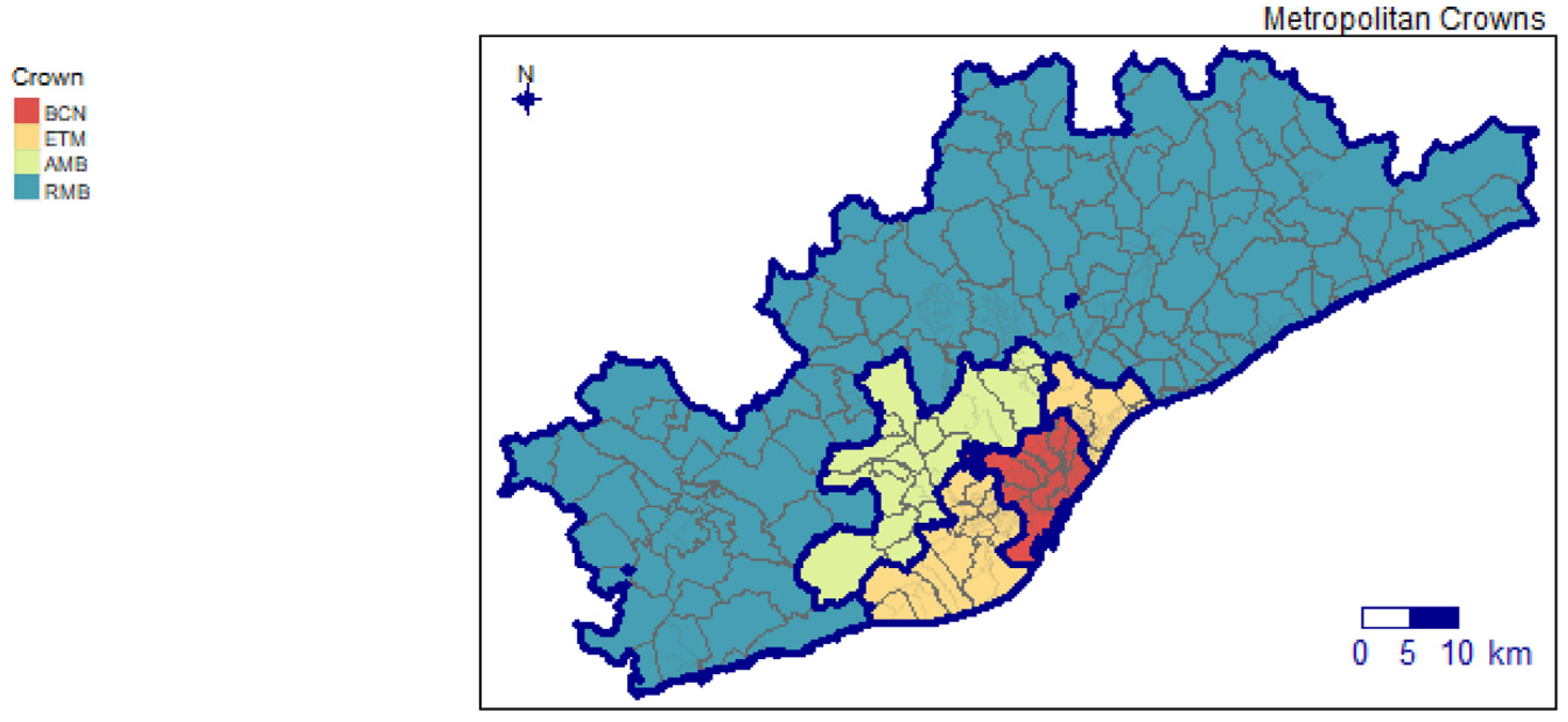
- The Municipality of Barcelona is divided into 10 macrozones, “TAZ-EMEF”, each corresponding to a district, as highlighted in Figure 1;
- In the RMB, each macrozone accounts for one municipality.
3.1. Study Data
- Data directly associated with each TAZ-EMO and data available from the local transportation authorities (Autoritat del Transport Metropolità, ATM, Barcelona, Spain), land registry system and Catalan Institute of Statistics (population census), as well as transport-related data available in GTFS documents. The land-use variables included were residential, commercial, industrial and other areas with services, using the roof area (m2) measured for each TAZ-EMO. Moreover, residential areas were divided into the following four types according to the terminology used in Barcelona for the different districts: old quarter, urban block (for example, Eixample neighbourhood), isolated blocks (found in suburban areas, such as l’Hospitalet de Llobregat), and individual detached and semidetached houses (for example, in Sant Cugat del Vallès). The sources of land use, transportation and socioeconomic data are provided in Table A2.
- Individual-level data from the Regional Transport Authority (AMB) (EMEF travel surveys) for the years 2018 to 2021, including age, gender (men and women only in the collected data) and education level.
3.2. Data Processing
3.3. Methodological Approach
- Afterward, the identified principal components were interpreted in terms of the contributions of the original variables.
- Hierarchical clustering analysis [56,58,59] was conducted in the space of the principal components to cluster the zones in terms of the similarities based on Ward linkages [60], as defined by the corresponding variables from the cluster profile analysis. The clusters were profiled according to the statistically most significant numeric variables and factors of the zones included in the analysis, which was based on the catdes() profiling method of the FactoMineR [55] library in R/RStudio [54,57].
- The optimal number of clusters was selected either retaining at least 50% of the data variability or according to the silhouette plot [61].
- To increase understanding and facilitate the interpretation of the results, clusters were mapped in the RMB.
- The EMEF survey respondents, together with their TAZ macrozone details, were identified in correspondence with their spatial cluster information, according to land use and the built environment. Afterward, we conducted a second clustering refinement within each spatial cluster for EMEF survey respondents based on their daily sequences to analyse their mobility behaviours, leading to subclusters based on the SA.
- The base analysis, defined in terms of the variables that were considered as neither gender nor fragmentation variables and located in blocks V1 to V14.
- The full analysis, including both the base analysis variables plus the modal uses according to gender (blocks V15 and V16) and gender fragmentation (blocks V17 to V20). The fragmentation indicators (see Appendix A for further details) were computed from the analysis of minute-by-minute sequences using the TraMinerR package [43,62] in RStudio [57].
4. Results
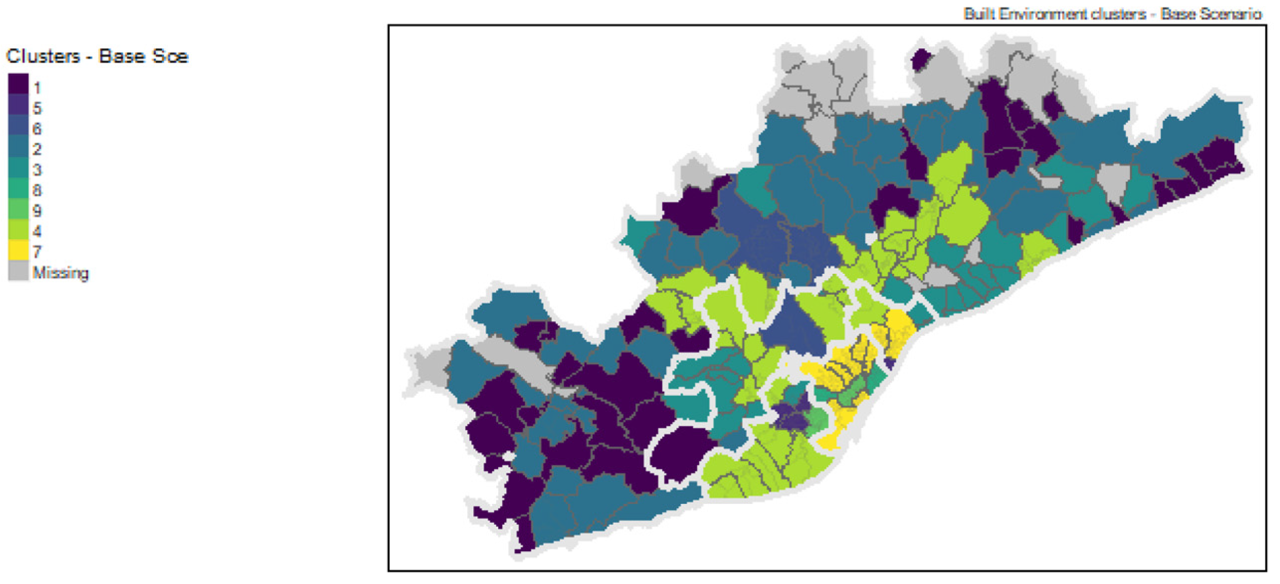
4.1. Base Analysis Results
- Axis 1. The first axis was positively related to population levels, jobs numbers, mixed land use/land use diversity and the number of bus, metro and commuter rail stops within each TAZ. This axis was negatively related to the mean travel time, at either the CBD or regional levels.
- Axis 2. The second axis was related to increasing travel times, for either any part of the metropolitan region or the CBD and the number of train stations.
- Axis 3. Percentage of dwelling areas in the zone.
- Axis 4. This axis was positively related to increases in the distance to access public transport facilities and increases in per capita income.
- Cluster 1. Municipalities in the rest of the RMB with low population densities and low land-use mix. Travel times to the CBD were above the mean in the RMB, either by private or public transportation, but access to public transport facilities was good. Public transport use was lower than the overall mean in the RMB.
- Cluster 2. The share of public transportation was less than the overall mean in the RMB. Although access to public transportation facilities was lower than the mean, bus stops were scarce.
- Cluster 3. Municipalities characterised by high residential use, a mean per capita income above the mean, short access times to public transportation facilities and good commutes to the CBD by car.
- Cluster 4. High incidence of detached houses, extensive use of nonmotorised transport modes and good access to the CBD via public transport.
- Cluster 5. A high share of public transportation, good access to the CBD via car or public transport and containing municipalities in the first crown (ETM).
- Cluster 6. Well-served by trains, with a high incidence of tertiary sector land use (e.g., businesses and restaurants) and higher mixed land use/land use diversity than the overall mean.
- Cluster 7. Municipalities with high population densities and land use diversity. They are well-served by buses and the metro. The number of bus stops is greater than the mean and the travel time to the city centre of Barcelona is less than the mean, either by private or public transportation. It is characterised by the traditional old city building type and contains municipalities in the first crown (ETM) and seven districts in Barcelona city.
- Cluster 8. Represented by many suburban neighbourhoods, with high-population and high land use diversity areas. It includes many schools/kindergartens and restaurants. The share of public transport was above the mean. This cluster also includes the “Sant Martí” and “les Corts” Districts located in Barcelona city.
- Cluster 9. Characterised by higher population and job densities and high land use diversity. It is well served by the metro, and the share of private transport is very low. It contains the “l’Eixample” District of Barcelona city and “l’Hospitalet de Llobregat”.
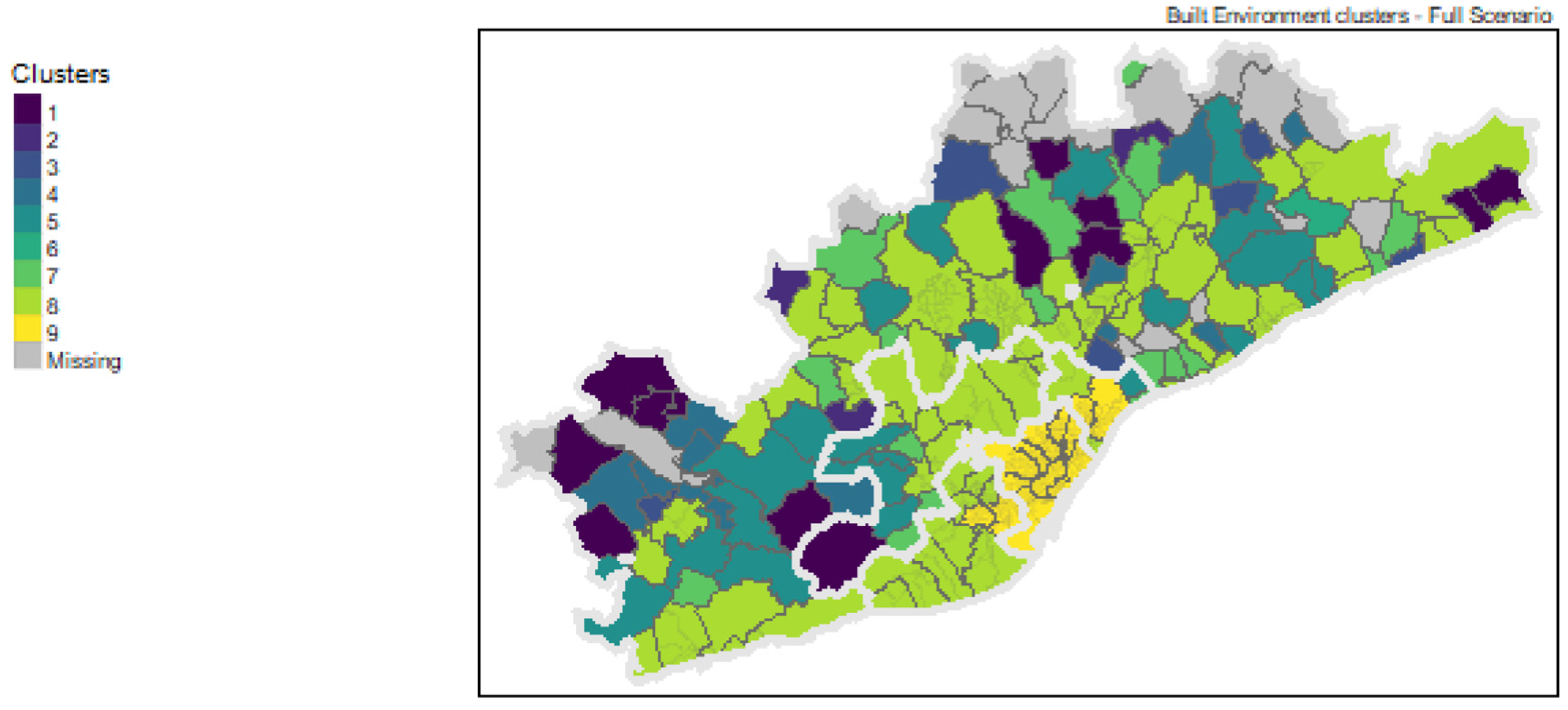
4.2. Full Analysis Results
- Axis 1. The first axis is positively related to population level, job numbers and high land use diversity, as well as the number of bus, metro and public train transport stops, with a high percentage of public transport use. This axis is negatively related to mean travel time to the CBD, either by private or public transport. This axis contraposes the density of activities inside and around Barcelona’s urban area to the travel time to the city centre. Municipalities, Barcelona city zones and the primary crown are located (ETM) on the positive part of this axis;
- Axis 2. This axis is related to the increasing turbulence and complexity experienced in 2018 to 2021 on the positive part of the axis;
- Axis 3. The third axis is related to the increasing turbulence and complexity experienced in 2018–2020 at opposite ends of the axes, being positive for men in 2019 and negative for women in 2018 and men in 2020;
- Axis 4. The fourth axis is related to increasing fragmentation indicators related to 2019 and 2021 on opposite ends of the axes, being positive for women in 2019 and negative for men in 2021 and women in 2020.
- Cluster 1. Travel time, by private or public transport, over the mean. Public transport use and male fragmentation indicators above the means in 2020.
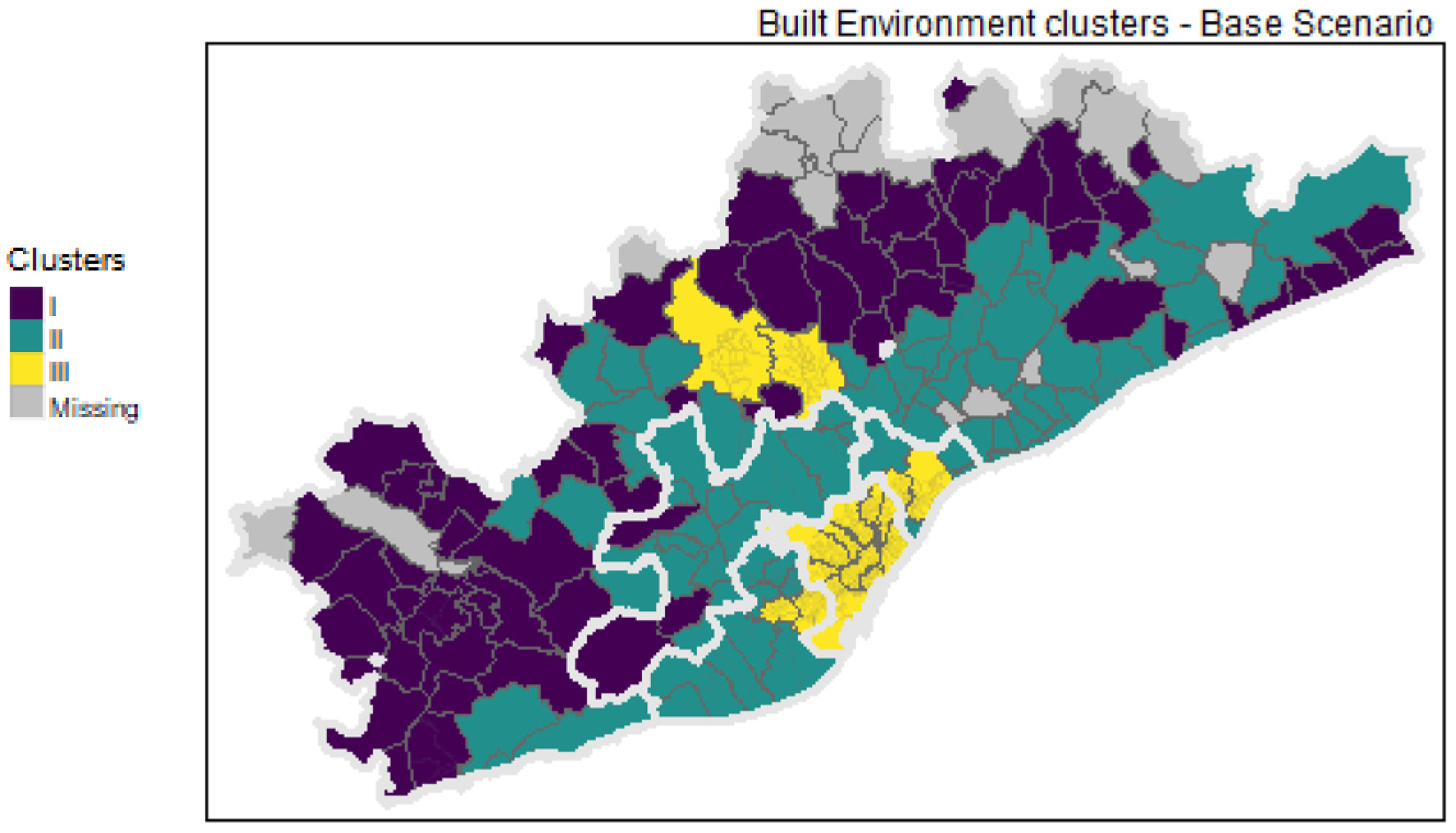
- Cluster 2. Entropy and travel times above the means for both men and women in 2021. Very low incidence of nonmotorised travel modes. Here, only one cluster was found, including small villages on the outskirts of the RMB, represented by the second-darkest blue in Figure 5.
- Cluster 3. Fully characterised by fragmentation indicators in different years.
- Cluster 4. Travel time by public transport and the share of private transport were very high. Turbulence and complexity were below the means in 2020.
- Cluster 5. Very high share of private vehicle use. Turbulence and complexity were below the means for women in 2020.
- Cluster 6. Turbulence and complexity considerably above the means in 2020, for both men and women. It only includes Vallgorguina, a municipality in the Montseny Natural Park area, north of the metropolitan area (third crown). During the strict COVID-19 lockdown measures in Spain, many residents in Barcelona temporarily moved to their holiday residences in this area (dark green in Figure 5).
- Cluster 7. Fragmentation indicators in 2019 and 2021 were above the means, and the private transport shares were also above the mean.
- Cluster 8. A per capita income below the mean and nonmotorised vehicle use above the mean. The cluster includes 63 municipalities, with medium-sized cities such as Sabadell, Terrassa, and Vilanova i la Geltrú (Figure 5 in light green).
- Cluster 9. Population level, job density and land use diversity above the means, including a high number of bus stops and services in general. It includes all districts in Barcelona city and the densely populated city of l’Hospitalet.
4.3. Full Analysis: Results Per Year
- 2018: 36.8% (Dim 1); 10.7% (Dim2); 8.6% (Dim3); 7.0% (Dim4); 63.2% (Total);
- 2019: 36.8% (Dim 1); 11.3% (Dim2); 8.7% (Dim3); 7.1% (Dim4); 63.9% (Total);
- 2020: 36.9% (Dim 1); 10.6% (Dim2); 8.6% (Dim3); 7.1% (Dim4); 63.1% (Total);
- 2021: 36.8% (Dim 1); 12.1% (Dim2); 7:4% (Dim3); 7.2% (Dim4); 63.5% (Total).
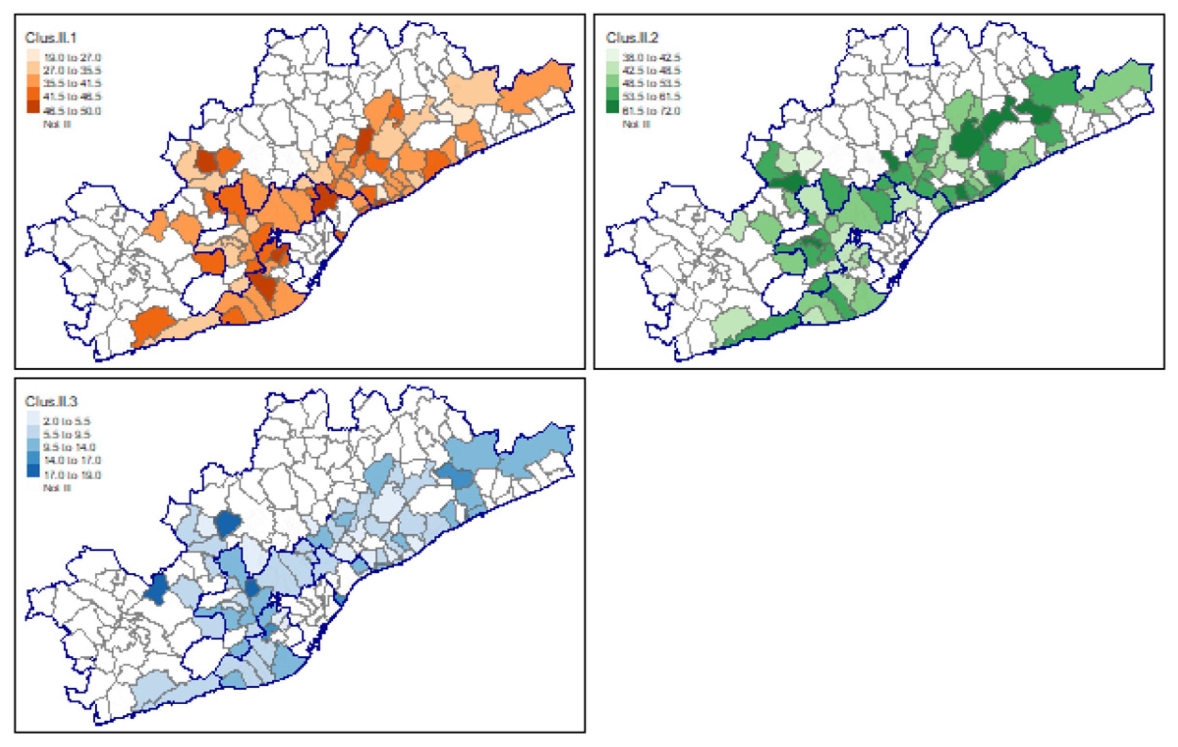
4.4. Full Analysis: Revisited
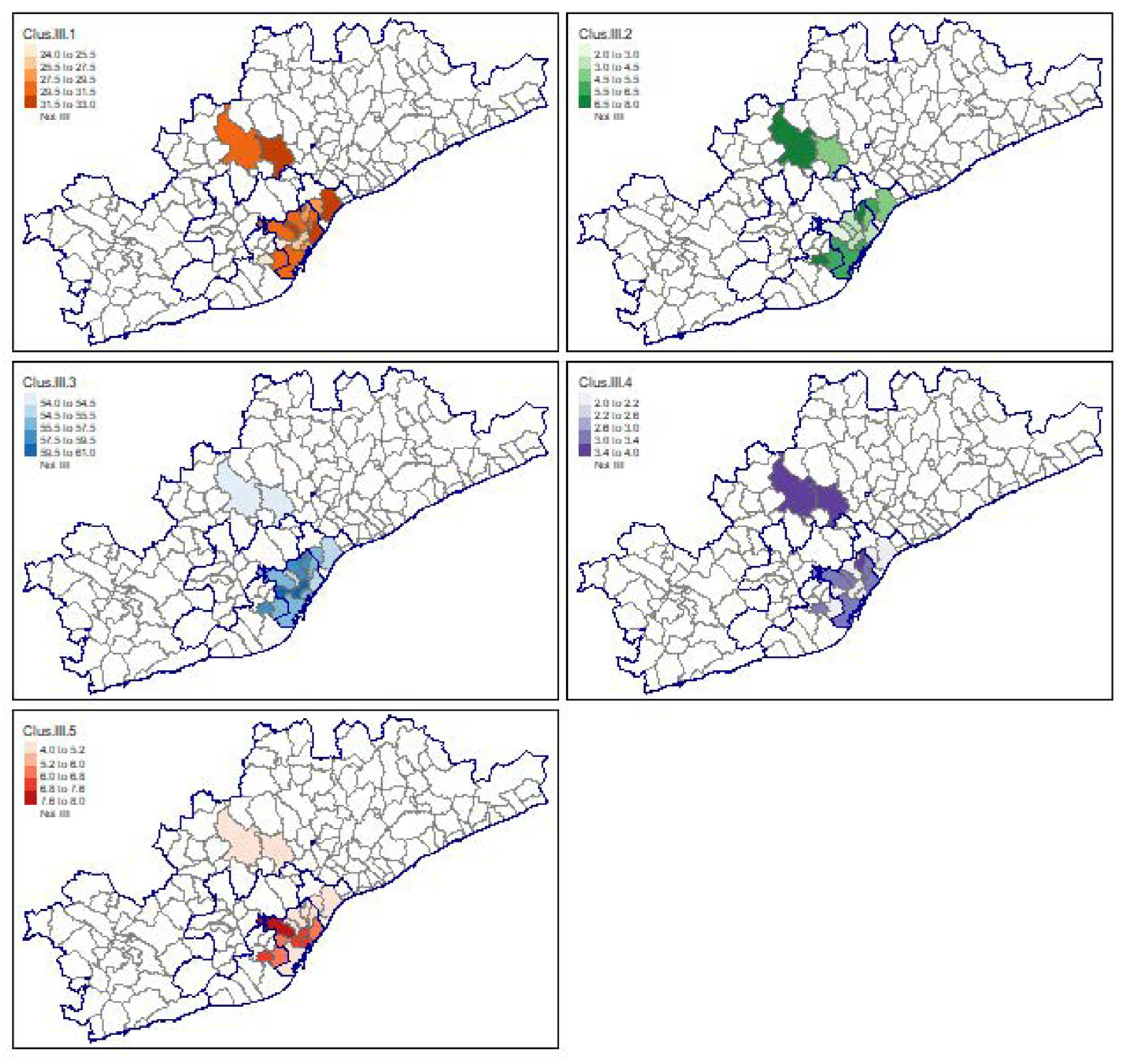
4.5. Optimal Spatial Clustering and Sequence Analysis (SA)
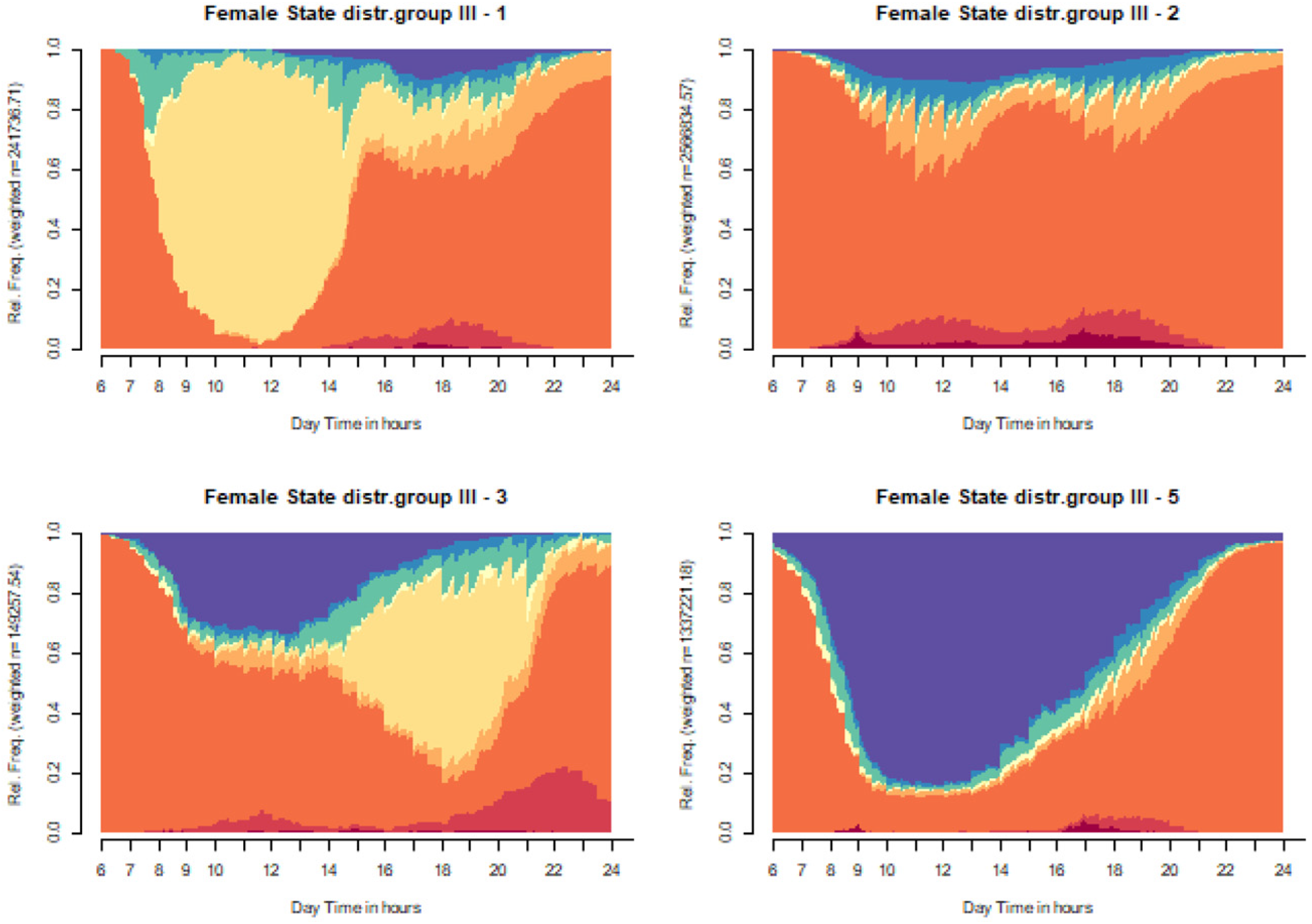
- Cluster III. 1—morning-shift workers, some of whom extend their shift throughout the day;
- Cluster III. 2—afternoon-shift workers;
- Cluster III. 3—a low incidence of work activity is highlighted, and the incidence of home-based activities is notable, but escorting and other recurrent (not work) activities occur during the day;
- Cluster III. 4—partial morning work and afternoon educational activities via public transport;
- Cluster III. 5—morning educational activities that, in some cases, extend into the afternoon, with almost no incidence of work activity or other recurrent late-afternoon activities.
5. Conclusions
Author Contributions
Funding
Institutional Review Board Statement
Informed Consent Statement
Data Availability Statement
Acknowledgments
Conflicts of Interest
Correction Statement
Appendix A

| Index | Description | Formula | No. |
|---|---|---|---|
| Entropy [43,44] | Provides a measure of variety in daily schedules and represents the proportion of total time spent in each state. is the proportion of occurrences of the ith state in the specific sequence, S is the number of potential states, is the sequence of daily activities defined from minute to minute and function log() refers to natural logarithm. Calculated based on the proportion of minutes allocated to each state during a day. This measure disregards the number of state changes and the specific ordering of states in the sequence. Visiting several states increases their entropy value whereas no state changes during the entire day is equal to a zero-entropy value. The potential value ranges depend on the number of states, with the maximum value achieved when the sequence evenly distributes time among all states. Therefore, a normalised entropy score is commonly used, dividing the entropy by the maximum entropy value, thus obtaining a range of 0 to 1. | (A1) | |
| Turbulence [42,44] | Measures the number of state recurrences and the variability in durations of daily activities. Based on sequence permanence and employs two components: the number of distinct subsequences that can be derived from the distinct state sequence; and the variance of consecutive time points spent in a distinct state. For a given sequence the turbulence considers is the number of distinct subsequences that can be extracted from the distinct state sequence, considering time precedence; is the variance for the state duration; and is the maximum variance, based on the sequence duration, computed as where n-1 is the number of transitions in the sequence and is the sequence duration divided by the number of distinct states in the sequence. | (A2) | |
| Complexity [42,43] | A normalised score [0, 1] based on the entropy and considers both the order of successive states, measured by transitions, and the distribution of different states. is the number of distinct transitions within a sequence, is the length of the sequence, is the entropy indicator, and is the maximum entropy in the sample. This index has a [0, 1] value, with 0 corresponding to no transitions (e.g., staying at home the entire day). A more sensitive indicator than entropy. | (A3) | |
| Travel time ratio [44] | Trade-offs that people make between travel time and activity time. Herein, TTR is calculated as total time spent on daily activities divided by the sum of the total time at home and the total time spent on daily activities ). TTR ranges from 0.5 (no trips made) to 1.0 (entire day spent away from home). | (A4) |
| Variable | Type | Source | Original Zoning System | Year | TAZ Data |
|---|---|---|---|---|---|
| Total roof area | Area | Land registry https://www.sedecatastro.gob.es/ (accessed on 11 November 2023) | Ground plots | 2019 | Roof area in m2 according to 16 types |
| Inhabitants by age group | Population | Population census IDESCAT | Census tracts | 2019 | Number of inhabitants by age group (four groups) |
| Inhabitants by education level | Population | Population census IDESCAT | Census tracts | 2011 | Number of inhabitants by education (four groups) |
| Income per Capita (Mean) | Population | IDESCAT (Catalan Institute of Statistics) | Census tracts | 2016 | Mean per capita income |
| Dwelling and dwelling size | Dwelling units | Population census AMB | Census tracts | 2011 | Number of dwelling units and dwelling size in four groups |
| Dwelling surface | Dwelling units | Population census AMB | Census tracts | 2011 | Number of dwelling units by dwelling surface group (four groups) |
| Parking areas | Parking | AMB | Ground plots | 2019 | m2 of ceiling |
| Residential type | Type of residential area | AMB | Ground plots | 2017 | m2 used by old city, blocks, urban blocks and isolated dwelling units |
| Services | Services | AMB | POIs | 2019 | Number of services according to 16 types |
| Educational buildings | Services | AMB | POIs | 2019 | Number of students |
| Urban bus stops | Transport data | GTFS | Dots | 2019 | Urban bus stops |
| Metropolitan bus stops | Transport data | GTFS | Dots | 2019 | Metropolitan bus stops |
| International bus stops | Transport data | AMB | Dots | 2019 | International bus stops |
| Metro stops | Transport data | GTFS | Dots | 2019 | Metro stops |
| Tram stops | Transport data | GTFS | Dots | 2019 | Tram stops |
| Taxi stops | Transport data | AMB | Dots | 2019 | Taxi stations |
| Train stations | Transport data | GTFS | Dots | 2019 | Number of train stations in each TAZ |
| Metropolitan train stations | Transport data | GTFS | Dots | 2019 | Number of metropolitan train stations in each TAZ |
References
- Lefebvre, H.; Hess, R.; Deulceux, S.; Weigand, G. Le Droit À La Ville; Economica-Anthropos: Paris, France, 2009; ISBN 9782717857085. [Google Scholar]
- Zieleniec, A. Lefebvre’s Politics of Space: Planning the Urban as Oeuvre. Urban. Plan. 2018, 3, 5–15. [Google Scholar] [CrossRef]
- Satterthwaite, D. A New Urban Agenda? Environ. Urban. 2016, 28, 3–12. [Google Scholar] [CrossRef]
- Vacchelli, E.; Kofman, E. Towards an Inclusive and Gendered Right to the City. Cities 2018, 76, 1–3. [Google Scholar] [CrossRef]
- UN-Habitat (Ed.) The New Urban Agenda|Urban Agenda Platform; UN-Habitat: Nairobi, Kenya, 2020; ISBN 978-92-1-132869-1. [Google Scholar]
- Rodrigue, J.P. The Geography of Transport Systems, 6th ed.; Taylor and Francis: London, UK, 2024; ISBN 9781003860327. [Google Scholar]
- Krauss, K.; Reck, D.J.; Axhausen, K.W. How Does Transport Supply and Mobility Behaviour Impact Preferences for MaaS Bundles? A Multi-City Approach. Transp. Res. Part. C Emerg. Technol. 2023, 147, 104013. [Google Scholar] [CrossRef]
- Abduljabbar, R.L.; Liyanage, S.; Dia, H. The Role of Micro-Mobility in Shaping Sustainable Cities: A Systematic Literature Review. Transp. Res. D Transp. Environ. 2021, 92, 102734. [Google Scholar] [CrossRef]
- Levy, C. Travel Choice Reframed: “Deep Distribution” and Gender in Urban Transport. Environ. Urban. 2013, 25, 47–63. [Google Scholar] [CrossRef]
- Kadi, J.; Matznetter, W. The Long History of Gentrification in Vienna, 1890–2020. City 2022, 26, 450–472. [Google Scholar] [CrossRef]
- Cooper, A.; Kurzer, P. Similar Origins – Divergent Paths: The Politics of German and Dutch Housing Markets. Ger. Polit. 2023, 32, 341–360. [Google Scholar] [CrossRef]
- Loomans, D. Long-Term Housing Challenges: The Tenure Trajectories of EU Migrant Workers in the Netherlands. Hous. Stud. 2023, 1–28. [Google Scholar] [CrossRef]
- Mejía-Dorantes, L.; Murauskaite-Bull, I. Transport Poverty—A Systematic Literature Review in Europe; EUR 31267 EN.; Publication Office of the European Union: Luxembourg, 2022; ISBN 978-92-76-58571-8. JRC129559. [Google Scholar]
- Ferrer-Ortiz, C.; Marquet, O.; Mojica, L.; Vich, G. Barcelona under the 15-Minute City Lens: Mapping the Accessibility and Proximity Potential Based on Pedestrian Travel Times. Smart Cities 2022, 5, 146–161. [Google Scholar] [CrossRef]
- Gil-Alonso, F.; López-Villanueva, C.; Thiers-Quintana, J. Transition towards a Sustainable Mobility in a Suburbanising Urban Area: The Case of Barcelona. Sustainability 2022, 14, 2560. [Google Scholar] [CrossRef]
- Montero, L.; Mejía-Dorantes, L.; Barceló, J. The Role of Life Course and Gender in Mobility Patterns: A Spatiotemporalsequence Analysis in Barcelona. Eur. Transp. Res. Rev. 2023, 15, 44. [Google Scholar] [CrossRef]
- Cubells, J.; Marquet, O.; Miralles-Guasch, C. Gender and Age Differences in Metropolitan Car Use. Recent Gender Gap Trends in Private Transport. Sustainability 2020, 12, 7286. [Google Scholar] [CrossRef]
- Rasouli, S.; Timmermans, H. Activity-Based Models of Travel Demand: Promises, Progress and Prospects. Int. J. Urban. Sci. 2014, 18, 31–60. [Google Scholar] [CrossRef]
- Alexander, B.; Ettema, D.; Dijst, M. Fragmentation of Work Activity as a Multi-Dimensional Construct and Its Association with ICT, Employment and Sociodemographic Characteristics. J. Transp. Geogr. 2010, 18, 55–64. [Google Scholar] [CrossRef]
- Couclelis, H. Pizza over the Internet: E-Commerce, the Fragmentation of Activity and the Tyranny of the Region. Entrep. Reg. Dev. 2006, 16, 41–54. [Google Scholar] [CrossRef]
- Alexander, B.; Hubers, C.; Schwanen, T.; Dijst, M.; Ettema, D. Anything, Anywhere, Anytime? Developing Indicators to Assess the Spatial and Temporal Fragmentation of Activities. Environ. Plan. B Urban. Anal. City Sci. 2011, 38, 678–705. [Google Scholar] [CrossRef]
- Little, J.; Peake, L.; Richardson, P. Introduction: Geography and Gender in the Urban Environment. In Women in Cities; Palgrave Macmillan: Basingstoke, UK, 1988; pp. 1–20. ISBN 978-1-349-19576-3. [Google Scholar]
- Law, R. Beyond ‘Women and Transport’: Towards New Geographies of Gender and Daily Mobility. Prog. Hum. Geogr. 1999, 23, 567–588. [Google Scholar] [CrossRef]
- Pratt, G.; Hanson, S. On the Links between Home and Work: Family-Household Strategies in a Buoyant Labour Market. Int. J. Urban. Reg. Res. 1991, 241–250. [Google Scholar] [CrossRef]
- Cresswell, T.; Uteng, T.P. Gendered Mobilities: Towards an Holistic Understanding. In Gendered Mobilities; Routledge: London, UK, 2016; pp. 1–12. ISBN 9781315584201. [Google Scholar]
- Gordon, P.; Kumar, A.; Richardson, H.W. Gender Differences in Metropolitan Travel Behaviour. Reg. Stud. 1989, 23, 499–510. [Google Scholar] [CrossRef]
- Ritschard, G. Measuring the Nature of Individual Sequences. Sociol. Methods Res. 2023, 52, 2016–2049. [Google Scholar] [CrossRef]
- Studer, M.; Ritschard, G. What Matters in Differences between Life Trajectories: A Comparative Review of Sequence Dissimilarity Measures on JSTOR. J. R. Stat. Soc. A 2016, 179, 481–511. [Google Scholar] [CrossRef]
- Hubers, C.; Dijst, M.; Schwanen, T. The Fragmented Worker? ICTs, Coping Strategies and Gender Differences in the Temporal and Spatial Fragmentation of Paid Labour. Time Soc. 2015, 27, 92–130. [Google Scholar] [CrossRef]
- Shi, H.; Goulias, K.G. Long-Term Effects of COVID-19 on Time Allocation, Travel Behavior, and Shopping Habits in the United States. J. Transp. Health 2024, 34, 101730. [Google Scholar] [CrossRef]
- Cheng, Y.T.; Lavieri, P.S.; Luiza Santos de Sá, A.; Astroza, S. Investigating the Effects of ICT Evolution and the COVID-19 Pandemic on the Spatio-Temporal Fragmentation of Work Activities. Transp. Res. Part. A Policy Pract. 2024, 187, 104192. [Google Scholar] [CrossRef]
- Abbott, A. Sequences of Social Events: Concepts and Methods for the Analysis of Order in Social Processes. Hist. Methods: A J. Quant. Interdiscip. Hist. 1983, 16, 129–147. [Google Scholar] [CrossRef]
- Abbott, A. Event Sequence and Event Duration: Colligation and Measurement. Hist. Methods: A J. Quant. Interdiscip. Hist. 1984, 17, 192–204. [Google Scholar] [CrossRef]
- Abbott, A.; Forrest, J. Optimal Matching Methods for Historical Sequences. J. Interdiscip. Hist. 1986, 16, 471. [Google Scholar] [CrossRef]
- Abbott, A.; Tsay, A. Sequence Analysis and Optimal Matching Methods in Sociology: Review and Prospect. Sociol. Methods Res. 2000, 29, 3–33. [Google Scholar] [CrossRef]
- Leszczyc, P.T.L.P.; Timmermans, H. Unconditional and Conditional Competing Risk Models of Activity Duration and Activity Sequencing Decisions: An Empirical Comparison. J. Geogr. Syst. 2002, 4, 157–170. [Google Scholar] [CrossRef]
- McBride, E.C.; Davis, A.W.; Goulias, K.G. Sequence Analysis of Place-Travel Fragmentation in California. In Mapping the Travel Behavior Genome; Elsevier: Amsterdam, The Netherlands, 2020; pp. 371–398. ISBN 9780128173404. [Google Scholar]
- Shi, H.; Su, R.; Xiao, J.; Goulias, K.G. Spatiotemporal Analysis of Activity-Travel Fragmentation Based on Spatial Clustering and Sequence Analysis. J. Transp. Geogr. 2022, 102, 103382. [Google Scholar] [CrossRef]
- Su, R.; McBride, E.C.; Goulias, K.G. Pattern Recognition of Daily Activity Patterns Using Human Mobility Motifs and Sequence Analysis. Transp. Res. Part. C Emerg. Technol. 2020, 120, 102796. [Google Scholar] [CrossRef]
- Goulias, K.G.; McBride, E.C.; Su, R. Life Cycle Stages, Daily Contacts, and Activity-Travel Time Allocation for the Benefit of Self and Others. In Mobility and Travel Behaviour Across the Life Course; Scheiner, J., Rau, H., Eds.; Edward Elgar Publishing: Cheltenham, UK, 2020; pp. 206–220. ISBN 9781789907803. [Google Scholar]
- McBride, E.; Davis, A.; Goulias, K. Exploration of Statewide Fragmentation of Activity and Travel and a Taxonomy of Daily Time Use Patterns Using Sequence Analysis in California. Transp. Res. Rec. 2020, 2674, 38–51. [Google Scholar] [CrossRef]
- Elzinga, C.H.; Liefbroer, A.C. De-Standardization of Family-Life Trajectories of Young Adults: A Cross-National Comparison Using Sequence Analysis. Eur. J. Popul. 2007, 23, 225–250. [Google Scholar] [CrossRef]
- Gabadinho, A.; Ritschard, G.; Studer, M.; Müller, N.S. Mining Sequence Data in R with the TraMineR Package: A User s Guide; Department of Econometrics and Laboratory of Geograpghy (University of Geneve): Geneve, Switzerland, 2011. [Google Scholar]
- McBride, E.; Davis, A.; Goulias, K. Fragmentation in Daily Schedule of Activities Using Activity Sequences. Transp. Res. Rec. 2019, 2673, 844–854. [Google Scholar] [CrossRef]
- Liao, T.F.; Bolano, D.; Brzinsky-Fay, C.; Cornwell, B.; Fasang, A.E.; Helske, S.; Piccarreta, R.; Raab, M.; Ritschard, G.; Struffolino, E.; et al. Sequence Analysis: Its Past, Present, and Future. Soc. Sci. Res. 2022, 107, 102772. [Google Scholar] [CrossRef]
- Rokach, L.; Maimon, O. Clustering Methods. In Data Mining and Knowledge Discovery Handbook; Springer: Berlin/Heidelberg, Germany, 2005; pp. 321–352. ISBN 978-0-387-25465-4. [Google Scholar]
- Grubesic, T.H.; Wei, R.; Murray, A.T. Spatial Clustering Overview and Comparison: Accuracy, Sensitivity, and Computational Expense. Ann. Assoc. Am. Geogr. 2014, 104, 1134–1156. [Google Scholar] [CrossRef]
- Lenz, B.; Nobis, C. The Changing Allocation of Activities in Space and Time by the Use of ICT—“Fragmentation” as a New Concept and Empirical Results. Transp. Res. Part. A Policy Pract. 2007, 41, 190–204. [Google Scholar] [CrossRef]
- Von Behren, S.; Hilgert, T.; Kirchner, S.; Chlond, B.; Vortisch, P. Image-Based Activity Pattern Segmentation Using Longitudinal Data of the German Mobility Panel. Transp. Res. Interdiscip. Perspect. 2020, 8, 100264. [Google Scholar] [CrossRef]
- Sidharthan, R.; Bhat, C.; Pendyala, R.; Goulias, K. Model for Children’s School Travel Mode Choice. Transp. Res. Rec. J. Transp. Res. Board 2011, 2213, 78–86. [Google Scholar] [CrossRef]
- Institut-Metropoli Working Day Mobility Surveys (EMEF)—Mobility Observatory in Catalonia (OMC)—ATM. Available online: https://omc.cat/en/w/surveys-emef (accessed on 8 September 2023).
- Montero, L.; Mejía-Dorantes, L.; Barceló, J. Applying Data Analytics to Analyze Activity Sequences for an Assessment of Fragmentation in Daily Travel Patterns: A Case Study of the Metropolitan Region of Barcelona. Sustainability 2023, 15, 14213. [Google Scholar] [CrossRef]
- PTV AG Germany VISUM 2020. Available online: https://ptvpartner.ro/sites/default/files/inline-files/Overview_Visum2020.pdf (accessed on 8 September 2023).
- R Development Core Team R: The R Project for Statistical Computing 2021. Available online: https://www.r-project.org/ (accessed on 8 September 2023).
- Husson, F.; Josse, J.; Lê, S.; Mazet, J. FactoMineR: An R Package for Multivariate Analysis. J. Stat. Softw. 2008, 25, 1–18. [Google Scholar]
- Husson, F.; Lê, S.; Pages, J. Exploratory Multivariate Analysis by Example Using R, 2nd ed.; CRC Press: Boca Raton, FL, USA, 2017; ISBN 9780367658021. [Google Scholar]
- RStudio-Team RStudio: Integrated Development for R. 2022. Available online: https://www.r-project.org/conferences/useR-2011/abstracts/180111-allairejj.pdf (accessed on 8 September 2023).
- Nielsen, F. Introduction to HPC with MPI for Data Science; Undergraduate Topics in Computer Science; Springer: Berlin/Heidelberg, Germany, 2016; ISBN 978-3-319-21902-8. [Google Scholar]
- Kaufman, L.; Rousseeuw, P.J. Finding Groups in Data; Wiley Series in Probability and Statistics; Wiley: Hoboken, NJ, USA, 1990; ISBN 9780471878766. [Google Scholar]
- Ward, J.H. Hierarchical Grouping to Optimize an Objective Function. J. Am. Stat. Assoc. 1963, 58, 236. [Google Scholar] [CrossRef]
- Rousseeuw, P.J. Silhouettes: A Graphical Aid to the Interpretation and Validation of Cluster Analysis. J. Comput. Appl. Math. 1987, 20, 53–65. [Google Scholar] [CrossRef]
- Gabadinho, A.; Ritschard, G.; Müller, N.S.; Studer, M. Analyzing and Visualizing State Sequences in R with TraMineR. J. Stat. Softw. 2011, 40, 1–37. [Google Scholar] [CrossRef]
- Lorente, E.; Codina, E.; Barceló, J.; Nökel, K. An Approach Based on Simulation and Optimisation for the Intermodal Dispatching of Public Transport and Ride-Pooling Services. Appl. Sci. 2023, 13, 3803. [Google Scholar] [CrossRef]
- UITP. Mobility as a Service; International Association of Public Transport: Brussels, Belgium, 2019. [Google Scholar]
- ITF Shared Mobility Simulations for Auckland. International Transport Forum Policy Papers; OECD Publishing: Paris, France, 2017; p. 114. [Google Scholar] [CrossRef]
- ITF Shared Mobility Simulations for Dublin. International Transport Forum Policy Papers; OECD Publishing: Paris, France, 2018; p. 95. [Google Scholar] [CrossRef]
- ITF Shared Mobility Simulations for Helsinki. International Transport Forum Policy Papers; OECD Publishing: Paris, France, 2017; p. 95. [Google Scholar] [CrossRef]
- Lorente, E.; Codina, E.; Barceló, J.; Nökel, K. Enhancing Sustainable Urban Intermodal Systems: Simulating the Effects of Key Parameters in Integrated Ride-Pooling and Public Transport. Sustainability 2024, 16, 5013. [Google Scholar] [CrossRef]
- Axhausen, K.W.; Gärling, T. Activity-based Approaches to Travel Analysis: Conceptual Frameworks, Models, and Research Problems. Transp. Rev. 1992, 12, 323–341. [Google Scholar] [CrossRef]
- Bhat, C.R.; Goulias, K.G.; Pendyala, R.M.; Paleti, R.; Sidharthan, R.; Schmitt, L.; Hu, H.H. A Household-Level Activity Pattern Generation Model with an Application for Southern California. Transportation 2013, 40, 1063–1086. [Google Scholar] [CrossRef]
- Kitamura, R.; Chen, C.; Pendyala, R.M. Generation of Synthetic Daily Activity-Travel Patterns. Transp. Res. Rec. 1997, 1607, 154–162. [Google Scholar] [CrossRef]
- Horni, A.; Charypar, D.; Axhausen, K.W. Variability in Transport Microsimulations Investigated with the Multi-Agent Transport Simulation MATSim. Arbeitsberichte Verk. Raumplan. 2011, 692. [Google Scholar] [CrossRef]
- Miller, E.J.; Roorda, M.J. Prototype Model of Household Activity-Travel Scheduling. Transp. Res. Rec. 2003, 1831, 114–121. [Google Scholar] [CrossRef]


| Concept | Definition and Calculation | Variable Name and Description |
|---|---|---|
| Residential density (V1) | The number of inhabitants per km2 and TAZ, calculated as a weighted mean for the TAZ-EMO data included in each TAZ macrozone. | densitypopm: mean population density. |
| Employment density (V2) | Defined in terms of roof surface, in m2, dedicated for the following categories: commercial, cultural, public use, primary and secondary education, industrial, warehouses, entertainment, restaurants and hotels and offices, calculated as weighted means and standard deviations based on the mean total m2 of roofs for each activity, considering the TAZ aggregation. | densityjobm: mean job density. |
| Mixed land use or land use diversity (V3) | Defined as the land-use mix (LUM) indicator, as follows: | diversity: weighted mean diversity. |
| (1) | ||
| where Pij is the proportion of land-use type j in transportation zone I, and n is the number of land-use types (residential, commercial, services, etc.) considered in this study (17), calculated as weighted means by population for each TAZ-EMO, in the combination process, included in each TAZ. | ||
| Residential type (V4) | Defined as the percentage of m2 in each of the four considered categories (old quarter, urban block, isolated block and detached dwelling unit) divided into the total m2 of residential use. | per_dwelling: percentage of residential use. Variables include typeblock, typeeix, typeold and typeaishh. |
| Accessibility of public transport (V5) | Accessibility of public transport by foot from the origin, calculated as the walking travel time (in minutes) from the centroid of the transportation zones in the Visum model [54] to transit stops in the zone, weighted by the total number of trips alighted at each stop. The aggregation of the Visum zones to the TAZs accounts for the mean weighted by population. | access2tpu |
| Access to destinations (V6) | Accessibility with public and private transport, obtained from transport assignments using a Visum model of the RMB [54] and skim matrices, omitting destinations that take longer than 150 min at which to arrive. | Wtt: mean travel time from origin to destination using any motorised mode. wttPu: mean travel time from origin to destination by public transport. wttPr: mean travel time from origin to destination by private transport. |
| CBD accessibility (V7) | Accessibility of CBDs (Districts 1/2) via public and private transportation. Data obtained from transport assignments from a Visum model of the RMB [54] and skim matrices, omitting destinations that take longer than 150 min at which to arrive. | wttD1.2: mean travel time from origin to CBD using any motorised mode. wttPuD1.2: mean travel time from origin to CBD using public transport. wttPrD1.2: mean travel time from origin to CBD using private transport. |
| Education (V8) | Number of kindergartens and primary and secondary educational centres within each TAZ. | school_places |
| Services (V9) | Commercial, leisure (including restaurants) and health services, calculated as the roof area, m2. | ser_comm, ser_horeca and ser_health |
| Average IPC (V10) | Average income per capita (IPC) at the TAZ level. The aggregation from Visum zones to the TAZs accounts for the mean IPCs weighted by population for each zone. | av_rent |
| No. of bus stops in each TAZ (V11) | Number of bus stops in each TAZ. | pbus |
| No. of metro stops (V12) | Number of metro stops in each TAZ. | pmetro |
| No. of commuter train stops (V13) | Number of commuter rail stops in each TAZ. | ptrain |
| No. of tramway stops (V14) | Number of tramway stops in each TAZ. | ptram |
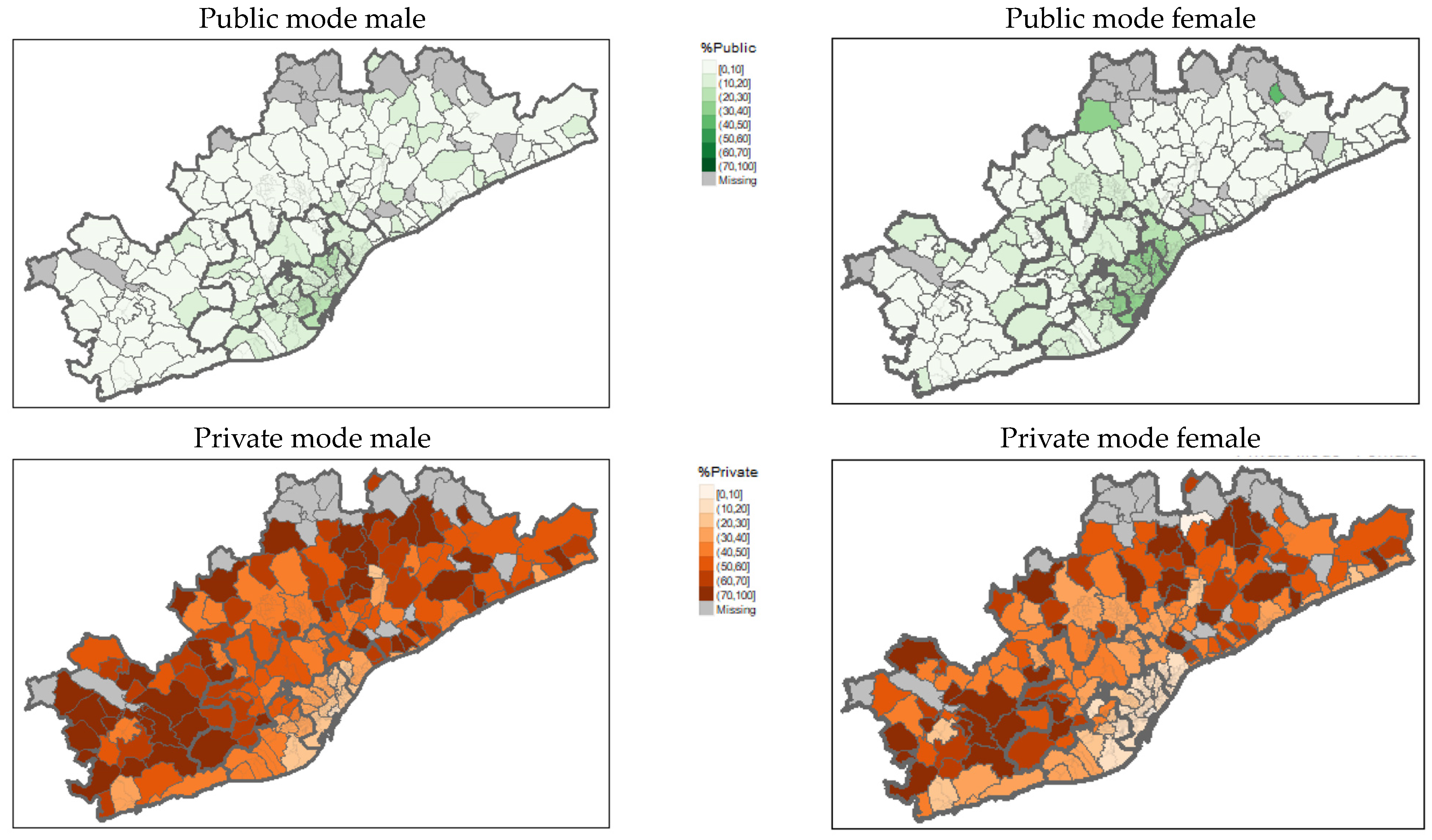
| Daily transport modes (V15) | Daily transport modes (in percentage) using private, public and other (bike, scooters, etc.) modes. Percentages were obtained from the totals at the TAZ level per year, with and without gender differentiation. | perprivate, perpublic and perother (without gender segregation); mperprivate, mperpublic and mperother (men); and fperprivate, fperpublic and fperother (women) |
| Percentages of the principal daily modes of transport by private, public and other modes (V16) | Percentages of the principal daily transportation modes of individuals using private, public and other modes, per year (2018, 2019, 2020 and 2021), with and without gender (women/men only) differentiation. | perdpprivate, perdppublic and perdprother (without gender segretation); mperdpprivate, mperdppublic and mperdpother (men); and fperdpprivate, fperdppublic and fperdpother (women) |
| Mean entropy (V17) | Per year (2018 to 2021) and by gender (women/men only) at the TAZ level. | entropy_year and entropy_year_gender |
| Mean turbulence (V18) | Per year (2018 to 2021) and by gender (women/men only) at the TAZ level. | turbulence_year and turbulence_year_gender |
| Mean complexity (V19) | Per year (2018 to 2021) and by gender (women/men only) at the TAZ level. | complexity_year and complexity_year_gender |
| Mean travel–time ratio (TTR) (V20) | Per year (2018 to 2021) and by gender (women/men only) at the TAZ level. | ttr_year and ttr_year_gender |
| Contribution to PCA Axes (%) | |||||||
|---|---|---|---|---|---|---|---|
| Variable | Dim.1 | Variable | Dim.2 | Variable | Dim.3 | Variable | Dim.4 |
| diversitym | 9.58 | wttPr | 18.15 | per_dwelling | 58.39 | access2tpu | 29.31 |
| school_places | 9.00 | ttPrD1.2 | 13.78 | av_rent | 9.62 | ptram | 22.94 |
| densitypopm | 8.87 | wttPu | 12.20 | wttPu | 7.92 | av_rent | 19.43 |
| pmetro | 8.73 | access2tpu | 8.79 | ttPuD1.2 | 6.42 | wttPu | 6.37 |
| densityjobm | 8.39 | av_rent | 8.52 | ptram | 4.55 | ptrain | 5.79 |
| ser_comm | 8.29 | ttPuD1.2 | 7.24 | ser_health | 3.84 | ttPuD1.2 | 4.99 |
| pbus | 7.91 | ser_comm | 5.70 | ptrain | 3.22 | per_dwelling | 4.10 |
| ser_health | 6.44 | ser_horeca | 5.16 | pmetro | 1.89 | wttPr | 1.81 |
| ttPrD1.2 | 6.27 | ptrain | 4.10 | densitypopm | 1.17 | school_places | 1.24 |
| ttPuD1.2 | 5.67 | diversitym | 3.10 | access2tpu | 1.05 | ttPrD1.2 | 1.15 |
| Contribution to PCA Axes (%) | |||||||
|---|---|---|---|---|---|---|---|
| Variable | Dim.1 | Variable | Dim.2 | Variable | Dim. 3 | Variable | Dim.4 |
| diversitym | 9.58 | wttPr | 18.15 | per_dwelling | 58.39 | access2tpu | 29.31 |
| school_places | 9.00 | ttPrD1.2 | 13.78 | av_rent | 9.62 | ptram | 22.94 |
| densitypopm | 8.87 | wttPu | 12.20 | wttPu | 7.92 | av_rent | 19.43 |
| pmetro | 8.73 | access2tpu | 8.79 | ttPuD1.2 | 6.42 | wttPu | 6.37 |
| densityjobm | 8.39 | av_rent | 8.52 | ptram | 4.55 | ptrain | 5.79 |
| ser_comm | 8.29 | ttPuD1.2 | 7.24 | ser_health | 3.84 | ttPuD1.2 | 4.99 |
| pbus | 7.91 | ser_comm | 5.70 | ptrain | 3.22 | per_dwelling | 4.10 |
| ser_health | 6.44 | ser_horeca | 5.16 | pmetro | 1.89 | wttPr | 1.81 |
| ttPrD1.2 | 6.27 | ptrain | 4.10 | densitypopm | 1.17 | school_places | 1.24 |
| ttPuD1.2 | 5.67 | diversitym | 3.10 | access2tpu | 1.05 | ttPrD1.2 | 1.15 |
| Contributions 2018 | Contributions 2019 | ||||||
|---|---|---|---|---|---|---|---|
| Dim.1 | Dim.2 | Dim.3 | Dim.4 | Dim.1 | Dim.2 | Dim.3 | Dim.4 |
| diversitym | entropy18m | complexity18f | fperother | diversitym | entropy19m | complexity19f | mperother |
| school_places | complexity18m | entropy18f | mperother | school_places | complexity19m | entropy19f | fperother |
| densitypopm | complexity18f | ttr18f | per_dwelling | densitypopm | ttr19m | ttr19f | mperprivate |
| pmetro | entropy18f | complexity18m | mperprivate | pmetro | complexity19f | complexity19m | wttPu |
| ser_comm | ttr18f | entropy18m | fperprivate | ser_comm | entropy19f | ttr19m | pmetro |
| pbus | ttr18m | turbulence18m | av_rent | pbus | turbulence19m | entropy19m | ttPuD1.2 |
| densityjobm | turbulence18m | turbulence18f | pmetro | densityjobm | ttr19f | turbulence19f | densitypopm |
| mperprivate | turbulence18f | ttr18m | ttPuD1.2 | mperprivate | turbulence19f | turbulence19m | densityjobm |
| ttPrD1.2 | av_rent | fperother | densitypopm | ttPuD1.2 | av_rent | access2tpu | fperprivate |
| ttPuD1.2 | wttPr | mperother | densityjobm | ttPrD1.2 | fperother | ttPrD1.2 | turbulence19f |
| Contributions 2020 | Contributions 2021 | ||||||
| Dim.1 | Dim.2 | Dim.3 | Dim.4 | Dim.1 | Dim.2 | Dim.3 | Dim.4 |
| diversitym | complexity20m | entropy20f | fperother | diversitym | entropy21f | mperother | complexity21m |
| school_places | complexity20f | complexity20m | mperother | school_places | ttr21f | fperother | entropy21m |
| densitypopm | entropy20m | ttr20f | mperprivate | densitypopm | complexity21f | turbulence21f | complexity21f |
| pmetro | entropy20f | entropy20m | fperprivate | pmetro | complexity21m | mperprivate | ttr21m |
| ser_comm | ttr20m | complexity20f | per_dwelling | ser_comm | entropy21m | complexity21f | entropy21f |
| pbus | ttr20f | ttr20m | turbulence20f | pbus | ttr21m | ttr21m | turbulence21m |
| densityjobm | turbulence20f | turbulence20m | pmetro | densityjobm | turbulence21f | entropy21m | ttr21f |
| mperprivate | turbulence20m | turbulence20f | av_rent | mperprivate | turbulence21m | fperprivate | turbulence21f |
| ttPrD1.2 | wttPu | access2tpu | densitypopm | ttPrD1.2 | av_rent | pmetro | fperother |
| ttPuD1.2 | per_dwelling | wttPu | densityjobm | ttPuD1.2 | per_dwelling | per_dwelling | access2tpu |
Disclaimer/Publisher’s Note: The statements, opinions and data contained in all publications are solely those of the individual author(s) and contributor(s) and not of MDPI and/or the editor(s). MDPI and/or the editor(s) disclaim responsibility for any injury to people or property resulting from any ideas, methods, instructions or products referred to in the content. |
© 2024 by the authors. Licensee MDPI, Basel, Switzerland. This article is an open access article distributed under the terms and conditions of the Creative Commons Attribution (CC BY) license (https://creativecommons.org/licenses/by/4.0/).
Share and Cite
Montero, L.; Mejía-Dorantes, L.; Barceló, J. Land Use, Travel Patterns and Gender in Barcelona: A Sequence Analysis Approach. Sustainability 2024, 16, 9004. https://doi.org/10.3390/su16209004
Montero L, Mejía-Dorantes L, Barceló J. Land Use, Travel Patterns and Gender in Barcelona: A Sequence Analysis Approach. Sustainability. 2024; 16(20):9004. https://doi.org/10.3390/su16209004
Chicago/Turabian StyleMontero, Lídia, Lucía Mejía-Dorantes, and Jaume Barceló. 2024. "Land Use, Travel Patterns and Gender in Barcelona: A Sequence Analysis Approach" Sustainability 16, no. 20: 9004. https://doi.org/10.3390/su16209004
APA StyleMontero, L., Mejía-Dorantes, L., & Barceló, J. (2024). Land Use, Travel Patterns and Gender in Barcelona: A Sequence Analysis Approach. Sustainability, 16(20), 9004. https://doi.org/10.3390/su16209004