Assessing the Scale Effects of Dynamics and Socio-Ecological Drivers of Ecosystem Service Interactions in the Lishui River Basin, China

Abstract

Grasping how scale influences the interactions among ecosystem services (ESs) is vital for the sustainable management of multiple ESs at the regional level. However, it is currently unclear whether the actual ES interactions and their driving mechanisms are consistent across different spatial and temporal scales. Therefore, using the Lishui River Basin of China as a case study, we analyzed the spatial and temporal distribution of five key ESs across three scales (grid, sub-watershed, and county) from 2010 to 2020. We also innovatively used Pearson correlation analysis, Self-organizing Mapping (SOM), and random forest analysis to assess the dynamic trends of trade-offs/synergies among ESs, ecosystem service bundles (ESBs), and their main socio-ecological drivers across different spatiotemporal scales. The findings showed that (1) the spatial distribution of ESs varied with land use types, with high-value areas mainly in the western and northern mountainous regions and lower values in the eastern part. Temporally, significant improvements were observed in soil conservation (SC, 3028.23–5023.75 t/hm²) and water yield (WY, 558.79–969.56 mm), while carbon sequestration (CS) and habitat quality (HQ) declined from 2010 to 2020. (2) The trade-offs and synergies among ESs exhibited enhanced at larger scales, with synergies being the predominant relationship. These relationships remained relatively stable over time, with trade-offs mainly observed in ES pairs related to nitrogen export (NE). (3) ESBs and their socio-ecological drivers varied with scales. At the grid scale, frequent ESB flows and transformations were observed, with land use/land cover (LULC) being the main drivers. At other scales, climate (especially temperature) and topography were dominant. Ecosystem management focused on city bundles or downstream city bundles in the east of the basin, aligning with urban expansion trends. These insights will offer valuable guidance for decision-making regarding hierarchical management strategies and resource allocation for regional ESs.

1. Introduction

In the last fifty years, a troubling decrease in two-thirds of ecosystem functions has occurred, resulting in significant negative effects on human well-being [1]. This situation highlights the urgent necessity for management interventions to ensure the sustainable utilization of natural resources. Ecosystem services (ESs) refer to the various benefits and functions that natural ecosystems provide to humanity, which can support human life and well-being both directly and indirectly [2]. Nonetheless, the implementation of mismatched ecological strategies can inadvertently harm ecosystems. For instance, managers often prioritize the optimization of a single ecosystem service (ES) without considering the interplay among different ESs, potentially causing a significant drop in the availability of other services [3]. Moreover, the complex interactions of ecological processes across different scales and times are frequently ignored when evaluating the dynamics of ESs at just one scale [4]. Thus, adopting a multi-scale approach to closely study ES interactions, pinpoint the driving factors, and elucidate the scale-dependent effects shaping these dynamics is essential. This approach is crucial for assisting decision-makers in developing scientific management strategies suited to local natural conditions.

Clarifying the ESs relationship is the primary task of formulating scientific ecological environment management strategies to effectively improve the living environment and enhance human well-being [5,6]. The complex interaction between ESs is mainly influenced by ES types, ES distribution patterns, and ecological management strategies [7], which typically encompass trade-offs, synergies, and ESBs [8]. The trade-off effect describes a scenario where enhancing one ES results in the deterioration of another. Conversely, synergy occurs when the supply of one ES changes—either increasing or decreasing—alongside a similar change in another service [9,10]. An ES bundle (ESB) is the spatiotemporal co-occurrence of multiple ESs [6,8], offering a novel approach to uncovering the relationships between them. It not only represents a specific level of ES supply but also reflects the relationships among ESs. Existing research has explored many methods to resolve complex ES interaction, e.g., Pearson or Spearman correlation analysis [11,12] and Bayesian Belief Networks [13,14] were primarily employed to evaluate the overall trade-offs and synergies among ESs. Meanwhile, bivariate spatial autocorrelation analysis [15] and geographically weighted regression [12] were commonly used to examine the spatial patterns of these interactions. The typical methods for identifying ESBs include principal component analysis [16,17], spatial autocorrelation analysis [18], K-means cluster analysis [13,19], and Self-organizing Mapping (SOM) [20]. For example, Shen et al. [21] used SOM to explore the interaction between various ESs in the Xiong’an New Area, which found that the spatial patterns of four ESBs were potentially related to land use cover. Existing studies found that SOM was an ideal analytical method for identifying ESBs [8] because it is characterized by high fault tolerance and strong inclusiveness at multiple spatial scales [22,23]. Apart from the in-depth exploration of ES interactions, revealing the main socio-ecological drivers behind the spatio-temporal variability of ESs or ESBs is also an important basis for formulating sustainable development strategies [24,25]. Therefore, analyzing the spatiotemporal pattern of ES interaction and its drivers from ecological and socioeconomic perspectives can offer valuable insights for developing tailored ecosystem management strategies for basins or regions [26,27].

Current research primarily addresses the spatial pattern and interaction of ESs at individual scales, such as grid, sub-watershed, and administrative regions [11,28,29,30]. However, scholars have gradually recognized that ES interactions have scale effects [8,31], and existing studies have begun to focus on conducting research from multi-time and multi-scale perspectives [8,12]. In terms of time scale, firstly, the tradeoff/synergy relationship of ES may strengthen, weaken, or shift direction over time [24,32]. Secondly, due to the change in natural resource endowment and socio-economic factors over time, various ESs have high dynamic changes, and the spatial distribution pattern of ESBs will also change over time [33,34]. Third, the process and feedback of ecosystem change have a time lag, such as the long cycle of support services and regulation services, and the factors affecting the supply of ES change with time [35,36]. Fourthly, identifying the temporal variation trends in ES interactions can help managers gain a deeper understanding of priority targets for future management strategies in ecosystems and land use planning [37]. Spatially, current research on ES interactions is primarily large and single-scale [17,38]. Research on the impact of different scales on ES interactions primarily focuses on comparing multiple spatial scales to reveal the spatial heterogeneity and scale effects of ES interactions [4,10,33]. However, there is a lack of studies that combine fine-scale analysis, such as grids, with large-scale analysis to identify ESBs [39]. Furthermore, the most critical aspect of sustainable ES management is exploring the trade-offs and synergies of ESs across multiple spatial scales [40]. This is because ES trade-offs and synergies exhibit scale-dependency [10,15]. For instance, Hou et al. [33] identified a tradeoff between habitat quality (HQ) and water yield (WY) at the pixel scale, with the direction of this interaction changing at the county scale. Therefore, to address the disconnect between ecological process scales and management practices, it is crucial to deeply investigate the dynamic changes in ES interactions across multiple spatiotemporal scales, which can enhance the understanding of ES dynamics and the optimization of management and decision-making [24].

The Lishui River Basin is an important tributary of the middle reaches of the Yangtze River in China and one of the four main tributaries that flow into Dongting Lake. As a typical representative of medium-scale watersheds, this region faces multiple socio-ecological development challenges, including water quality degradation, soil erosion, and ecological imbalance, due to intensified industrial and agricultural activities as well as steep terrain [41,42]. Given its typicality, this area has garnered attention as a focal point for research on fragile ecological environments, yielding a wealth of research outcomes [43,44], while few studies have considered the spatio-temporal evolution of ESs at multiple scales. Moreover, in quantitative studies of drivers, the fact that the response of ESs or ESBs to influencing factors may have a scaling effect is often overlooked [45]. The shortcomings of these studies hinder a thorough grasp of the intricate relationships within ecosystems and the spatial–temporal patterns of ecological function zoning. Therefore, this study explores the dynamic trends of ES interactions and their driving mechanisms across multiple spatiotemporal scales, integrating fine-scale analysis with large-scale perspectives. This study will provide a supplementary perspective on scale effects research, enhancing the understanding of the complexity and dynamics of ESs. Our objectives were to (1) reveal the spatio-temporal heterogeneity of ESs and the tradeoff/synergistic of ESs pairs at three scales, (2) identify ESBs and their spatio-temporal variation trends, and (3) determine the dominant drivers affecting the spatio-temporal distribution of ESBs. This endeavor aimed to furnish valuable insights for regional land use policy regulation, ecological compensation strategies, and the hierarchical management of ecological assets.

2. Materials and Methods

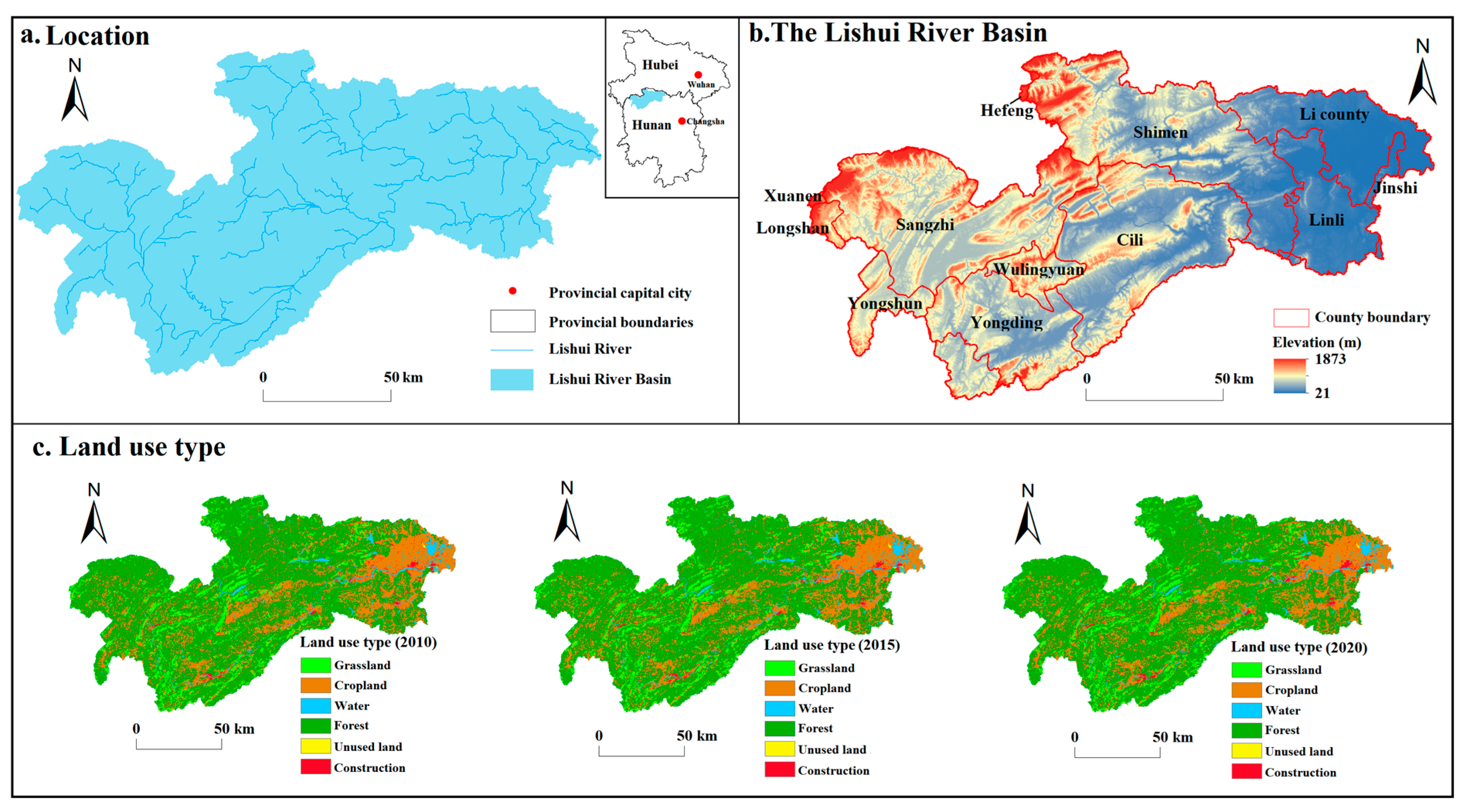
2.1. Study Area

The Lishui River Basin (29°30′ N–30°12′ N, 109°30′ E–112°0′ E) is located in the northwest of Hunan Province, China, and is an important tributary of the Yangtze River Basin. This basin originates from the Wuling Mountain Range in Hunan Province and flows through areas such as Zhangjiajie and Changde, eventually emptying into Dongting Lake (Figure 1). The main stream is 390 km long, covering a watershed area of 1.85 × 10⁴ km². The annual average water resources of the basin amount to 1.68 × 10¹⁰ m³, accounting for 9.9% of the total water storage in Hunan Province [42]. In the subtropical humid seasonal climate zone, the basin has an average annual temperature of about 16.5 °C and receives between 1254 and 1396.9 mm of precipitation annually. Vegetation within the basin predominantly comprises evergreen broad-leaved forests, which are concentrated in the headwaters of the upstream tributaries. However, the vegetation is relatively sparse in the midstream and downstream areas, leading to lower ecological benefits [41]. It is noteworthy that the construction land in the downstream regions of the basin has gradually expanded over time (Figure 1c and Figure S1). Steep slopes are relatively common within the basin, and the terrain gradually decreases in elevation from the northwest to the southeast. The extensive cultivation of sloping lands has led to severe soil erosion within the region [42].

2.2. Data Source and Processing

Spatial assessment of ESs and driving factors using multiple datasets in the Lishui River Basin. The study incorporated a variety of datasets, including satellite imagery, digital elevation model (DEM), land use/land cover (LULC), meteorological data, and socio-economic data pertaining to 2010, 2015, and 2020 (

Table 1. Data sources.

Data	Data Source	Spatial Resolution	Year	Related Model
Rain (annual average precipitation, annual total precipitation)	China Meteorological Data Network (https://data.cma.cn) and Global Climate Database (http://www.worldclimate.com/), accessed on 13 June 2023	1000 m	2010, 2015, 2020	WY, NDR
Root restricting layer depth	Defined from land use types and InVEST user’s guide	30 m	2020	WY
Digital elevation model	Geospatial Data Cloud (http://www.gscloud.cn/), accessed on 9 January 2024	30 m	2020	NDR, SDR
Plants’ available water content	Defined from land use types and InVEST user’s guide	30 m	2020	WY
Rainfall erosivity	https://gda.bnu.edu.cn/sypt/sjgx/tdlytdfgsjj/index.html, accessed on 7 May 2024	1000 m	2010, 2015, 2020	SDR
Evapotranspiration	The National Tibetan Plateau Data Center (https://data.tpdc.ac.cn/zh-hans/data/8b11da09-1a40-4014-bd3d-2b86e6dccad4), accessed on 13 June 2023	1000 m	2010, 2015, 2020	WY
Soil erodibility	https://gda.bnu.edu.cn/sypt/sjgx/tdlytdfgsjj/index.html, accessed on 23 May 2024	30 m	2020	SDR
Watersheds	https://www.resdc.cn/DOI/DOI.aspx?DOIID=44, accessed on 29 June 2023	1	2019	NDR, SDR, WY
LULC	Data Center for Resources and Environmental Sciences, Chinese Academy of Sciences (https://www.resdc.cn/), accessed on 6 February 2024	30 m	2010, 2015, 2020	CSS, HQ, NDR, SDR, WY,
Soil data	The National Tibetan Plateau Data Center (https://data.tpdc.ac.cn/), accessed on 16 June 2023	1000 m	2010	NDR, SDR, WY
Carbon density data	Derived from Chinese scientific data (http://csdata.org/), accessed on 5 June 2024	1000 m	2020	CSS
Biophysical Table	Based on literature and field studies, including LULC_veg, root_depth, Kc (the plant evapotranspiration coefficient), load of nutrients, and efficiency of nutrient retention, etc.	1	2010, 2015, 2020	NDR, SDR, WY
Mean annual temperature	China Meteorological Data Network (https://data.cma.cn), accessed on 18 October 2023	1000 m	2010, 2015, 2020	Some driving factors
Population density (POP)	WorldPop (https://www.worldpop.org/), accessed on 24 October 2023	1000 m	2010, 2015, 2020
Gross Domestic Product (GDP)	National Earth System Science Data Center (http://www.geodata.cn/data/datadetails.html?dataguid=844414&docid=6666), accessed on 24 October 2023	1000 m	2010, 2015, 2020

CSS, Carbon Storage and Sequestration; HQ, habitat quality; SDR, Sediment Delivery Ratio; NDR, Nutrient Delivery Ratio; WY, water yield, the same below; LULC, land use/land cover.

). Specifically, the extraction of the watershed and sub-watershed layers primarily referenced the research by Xu et al., mainly based on the DEM of the basin [46]. Moreover, to maintain data consistency, we unified raster data with different spatial resolutions by projecting them to the Asia_North_Albers_Equal_Area_Conic_China coordinate system. ArcGIS 10.7 was then used to resample the data to a resolution of 30 m for quantifying ESs and socio-ecological drivers.

2.3. Methods

In our study, we analyzed the spatiotemporal heterogeneity and socio-ecological drivers of ESBs in the Lishui River Basin from the following aspects (Figure 2). Initially, we quantified the spatiotemporal heterogeneity of ESs across various times and scales. Subsequently, we elucidated the ES trade-offs/synergies and their scale effects. Then, the ESBs at different spatiotemporal scales were analyzed. Finally, the main socio-ecological drivers leading to the spatio-temporal distribution of ESBs were identified.

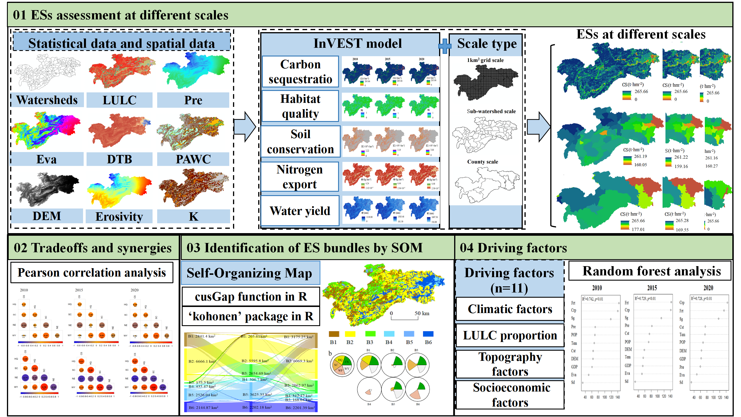
2.3.1. Quantification of ESs

In this study, five ESs were identified using specific criteria: (1) the classification of these ESs was consistent with the Millennium Ecosystem Assessment (MEA) [47]; (2) ability to represent both natural and socio-economic conditions of the study area, which is primarily dominated by forest and severely affected by soil erosion; (3) key ESs listed in the ecological functional areas of Dongting Lake Basin and Hunan Province; and (4) data availability and feasibility. Ultimately, five ESs were selected (

Table 2. Methodology used to quantify ESs in InVEST model [12,49,50].

Categories.	Ecosystem Services	Methods	Main Equation	Remarks	References
Provisioning  services	Water yield	WY	Equation (1)	Yx: annual water on grid x; AET: evapotranspiration; P: annual precipitation.	[12,51,52]
Regulating services	Nitrogen export	NDR	Equation (2)	${\mathrm{X}}_{{\mathrm{e}\mathrm{x}\mathrm{p}\mathrm{o}\mathrm{r}\mathrm{t}}_{\mathrm{t}\mathrm{o}\mathrm{t}}}$: total nutrient export; loadsurf,i and loadsubs,i: local runoff potential. NDRsurf,i and NDRsubs,i: nutrient delivery factors of surface and subsurface runoff.	[11,53]
	Soil conservation	SDR	Equation (3)	SCr: actual soil erosion; SCp: potential soil erosion; R: rainfall erosivity; K: soil erodibility. LS: slope length; P: conservation of soil and water; C: vegetation cover.	[54,55,56]
	Carbon sequestration	CSS	Equation (4)	${\mathrm{C}}_{\mathrm{t}\mathrm{o}\mathrm{t}}$: total CS; ${\mathrm{C}}_{\mathrm{a}\mathrm{b}\mathrm{o}\mathrm{v}\mathrm{e}}$: carbon in aboveground biomass; ${\mathrm{C}}_{\mathrm{b}\mathrm{e}\mathrm{l}\mathrm{o}\mathrm{w}}$: carbon in belowground biomass; ${\mathrm{C}}_{\mathrm{s}\mathrm{o}\mathrm{i}\mathrm{l}}$: soil carbon; ${\mathrm{C}}_{\mathrm{d}\mathrm{e}\mathrm{a}\mathrm{d}}$: carbon in dead matter.	[19,22,57,58,59,60]
Supporting service	Habitat quality	HQ	Equation (5)	${\mathrm{Q}}_{\mathrm{x}\mathrm{j}}$: HQ value of grid x; ${\mathrm{H}}_{\mathrm{j}}$: habitat suitability of LULC type j; ${\mathrm{D}}_{\mathrm{x}\mathrm{j}}$: habitat degradation degree; z: scaling parameter; k: the half-saturation constant.	[37,61]

The biophysical tables and parameters (Supplementary Materials, Tables S1–S6) necessary for the model were sourced from the InVEST User Guide [62] and relevant research findings from similar regions [50,63].

), including regulating services (carbon sequestration, CS; soil conservation, SC; nitrogen export, NE), supporting services (HQ), and provisioning services (WY). The evaluation of those ESs primarily entailed quantitative simulation using sub-modules within the Integrated Valuation of Ecosystem Services and Trade-offs (InVEST) model. Notably, NE can reflect water purification (WP) capacity, where higher nitrogen output indicates lower WP capacity [48]. Details of the primary algorithms used in each module can be found in Supplementary Materials.

$${\mathrm{Y}}_{\mathrm{x}}=(1-{\displaystyle \frac{{\mathrm{A}\mathrm{E}\mathrm{T}}_{\mathrm{x}}}{{\mathrm{P}}_{\mathrm{x}}}})\times {\mathrm{P}}_{\mathrm{x}}$$

(1)

$${\mathrm{X}}_{{\mathrm{e}\mathrm{x}\mathrm{p}\mathrm{o}\mathrm{r}\mathrm{t}}_{\mathrm{t}\mathrm{o}\mathrm{t}}}={\sum }_{\mathrm{i}}\left({\mathrm{l}\mathrm{o}\mathrm{a}\mathrm{d}}_{\mathrm{s}\mathrm{u}\mathrm{r}\mathrm{f},\mathrm{i}}\times {\mathrm{N}\mathrm{D}\mathrm{R}}_{\mathrm{s}\mathrm{u}\mathrm{r}\mathrm{f},\mathrm{i}}+{\mathrm{l}\mathrm{o}\mathrm{a}\mathrm{d}}_{\mathrm{s}\mathrm{u}\mathrm{b}\mathrm{s},\mathrm{i}}\times {\mathrm{N}\mathrm{D}\mathrm{R}}_{\mathrm{s}\mathrm{u}\mathrm{b}\mathrm{s},\mathrm{i}}\right)$$

(2)

$$\begin{array}{ll}\mathrm{S}\mathrm{C}& =\mathrm{R}\mathrm{K}\mathrm{L}\mathrm{S}\mathrm{x}-\mathrm{U}\mathrm{S}\mathrm{L}\mathrm{E}\mathrm{x}\\ & =\mathrm{R}\times \mathrm{K}\times \mathrm{L}\mathrm{S}\times (1-\mathrm{C}\times \mathrm{P})\end{array}$$

(3)

$${\mathrm{C}}_{\mathrm{t}\mathrm{o}\mathrm{t}}={\mathrm{C}}_{\mathrm{a}\mathrm{b}\mathrm{o}\mathrm{v}\mathrm{e}}+{\mathrm{C}}_{\mathrm{b}\mathrm{e}\mathrm{l}\mathrm{o}\mathrm{w}}+{\mathrm{C}}_{\mathrm{s}\mathrm{o}\mathrm{i}\mathrm{l}}+{\mathrm{C}}_{\mathrm{d}\mathrm{e}\mathrm{a}\mathrm{d}}$$

(4)

$${\mathrm{Q}}_{\mathrm{x}\mathrm{j}}={\mathrm{H}}_{\mathrm{j}}\times \left(1-{\displaystyle \frac{{\mathrm{D}}_{\mathrm{x}\mathrm{j}}^{\mathrm{z}}}{{\mathrm{D}}_{\mathrm{x}\mathrm{j}}^{\mathrm{z}}+{\mathrm{k}}^{\mathrm{z}}}}\right)$$

(5)

2.3.2. Unit Scale Division

The three spatial scales (grid scale, small watershed scale, and county scale) were delineated using ArcGIS 10.7. The specific steps are as follows: First, the grid scale was created by using the “Create Fishnet” function in the Sampling Tool of ArcGIS 10.7 to generate grids with a side length of 1 km. Subsequently, based on the DEM layer and the county administrative boundaries, the small-watershed and county scales were delineated, respectively. To quantify ESs at varying spatial scales, the “Zonal Statistics” tool in ArcGIS 10.7 was utilized to determine the average values.

2.3.3. Data Calculation and Sampling

All the data at the grid scale could be used for statistical analysis; however, sub-watershed and county boundaries were not regular squares like the grid. Simply averaging all the raster data within each cell, as performed in previous studies, may lead to bias in the “Zonal Statistics” results at the sub-watershed and county scales. Therefore, we adopted the random sampling technique in ArcGIS 10.7 to collect samples of ESs and driving factors at the sub-watershed and county scales. Random sampling can minimize sample bias and error, making the samples more representative of the overall characteristics, thus improving the accuracy and precision of the data [64]. First, “Create random points” in ArcGIS 10.7 was used to randomly create sample points at the raster layer, creating 5000 sample points in each county and 1000 sample points in each sub-watershed, each sample point containing 16 variables (5 ESs, 11 driver factors). Secondly, by using the “Extract Multiple Values to Points” tool in ArcGIS 10.7 and excluding samples with null values, the sample size for each variable was 60,000 at the county scale and 68,000 at the sub-watershed scale. Finally, the trade-offs/synergies of ESs, SOM, and driving mechanisms were analyzed using sample point data.

2.3.4. Quantification of Trade-Offs/Synergies Among ESs

To clarify the trade-offs and synergies between the five ESs at different scales, we first conducted a statistical analysis of the data obtained from the sample point data of the ESs. Then, we quantified the correlations between the ESs at different scales. The Pearson correlation analysis in R 4.3.3 was utilized to assess the overall tradeoff and synergy among ESs, which was a commonly used quantitative method for determining the direction and strength of ES interaction [65,66]. The correlation coefficients between two ESs can be positive or negative, indicating synergistic and trade-off relationships, respectively.

2.3.5. Identification of ES Bundles

We used SOM to identify ESBs at all scales. Different from traditional mathematical methods, this approach employs an unsupervised neural network approach that integrates principal component analysis with K-means clustering. The topological structure of the input space is retained by the nearest neighbor relation function, and spatial information is added to the analysis. The network is gradually optimized by using competitive learning strategies and relying on the competition among neurons to realize classification processing. Each grid, sub-watershed, and county can be assigned to the different or same ESB according to their spatial ES similarity [23,67]. In implementing SOM, first of all, we used standardized ES values of the same scale to make the ESBs of the three depicted times that are consistent and comparable. Secondly, five kinds of ES data were processed without dimension. Then, the optimal number of bundles was identified using the cusGap function in R 4.3.3. Finally, we performed the SOM analysis utilizing the “kohonen” package in the same version of R 4.3.3 software and mapped ESBs spatial distribution, time dynamic transition, and ES rose wind direction.

2.3.6. Analysis of Socio-Ecological Drivers

Driving Factors Selection

We synthesized representative socio-ecological drivers selected from previous relevant studies [41,44], combined with the regional environment and non-collinearity of the Lishui River Basin, and established an index system affecting the spatial differentiation of ESBs. Herein, there are 11 influencing factors, including four types: climate, LULC, topography, and socio-economic factors (

Table 3. The abbreviation of social–ecological factors.

Category	Indicator	Abbreviation
Proportion of land use types	Forest proportion	Frt
	Cropland proportion	Crp
	Construction proportion	Cst
Climatic	Annual average temperature	Tem
	Mean annual precipitation	Pre
	Evapotranspiration	Eva
Topographic factors	Elevation	DEM
	Slope gradient	Sg
	Slope direction	Sd
socio-economic factors	Population density	POP
	Gross domestic product	GDP

). The climatic factors included evapotranspiration, mean annual precipitation, and annual average temperature. Topographic factors consist of elevation, slope direction, and slope gradient. Additionally, with reference to previous studies, socio-economic factors were selected [68], including gross domestic product and population density. The land cover included the forest proportion, cropland proportion, and construction proportion.

Random Forest Analysis

As far as we know, this study was one of the few that utilized the random forest model to investigate the significance of drivers affecting the spatiotemporal distribution of ESBs. Specifically, we first performed a statistical analysis on the samples of 11 drivers, along with the spatial distribution types of ESBs that were previously obtained. Subsequently, we used the spatial distribution of drivers as a predictor and the spatial distribution types of ESBs as a classification result. Compared to methods such as neural networks and geostatistics, the random forest model provides a more stable and accurate evaluation of each predictor’s relative importance in ESB classification across various scales [69,70,71,72]. Additionally, we used the random forest model to evaluate how these drivers affect ESB classification over time. All analyses were conducted with the ‘randomForest’ package in R 4.3.3.

2.3.7. Other Statistic Analysis

The SPSS software (IBM SPSS Statistics 23) was used to conduct one-way ANOVA (Analysis of Variance), Fisher LSD (Least Significant Difference) test, and mean ± standard deviation, aiming at the significant differences in ESs between different spatial scales and different temporal scales.

3. Results

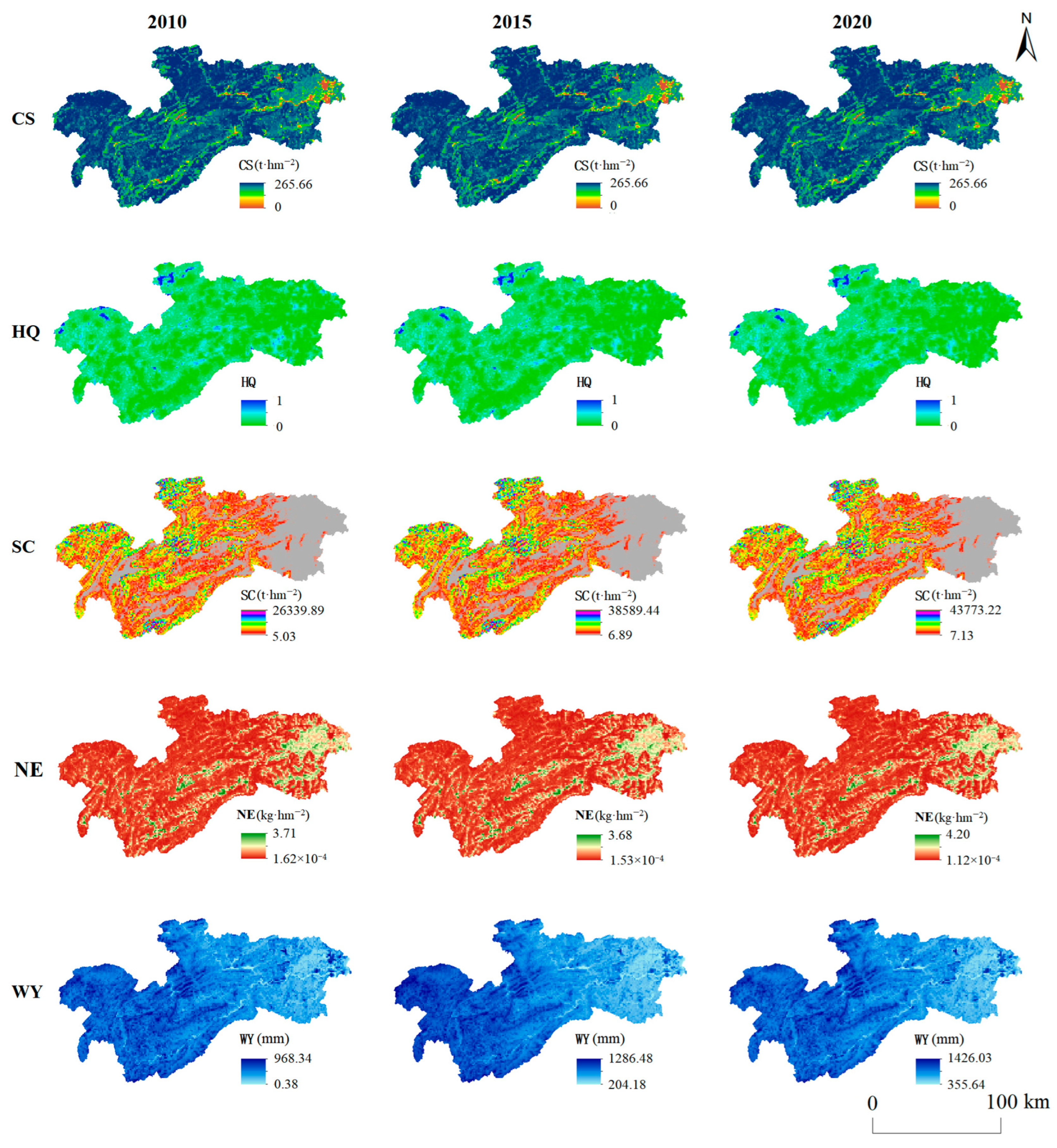
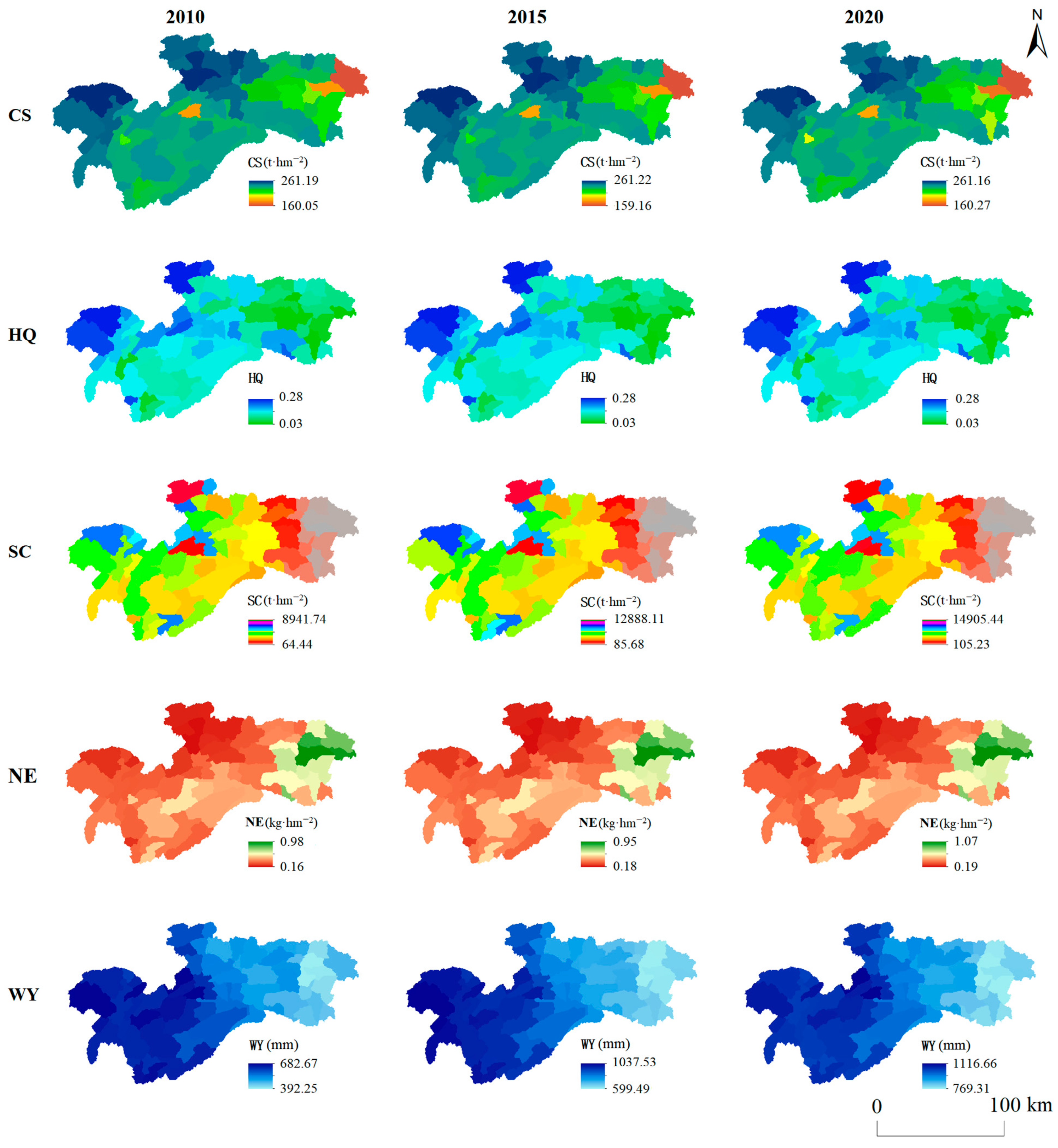
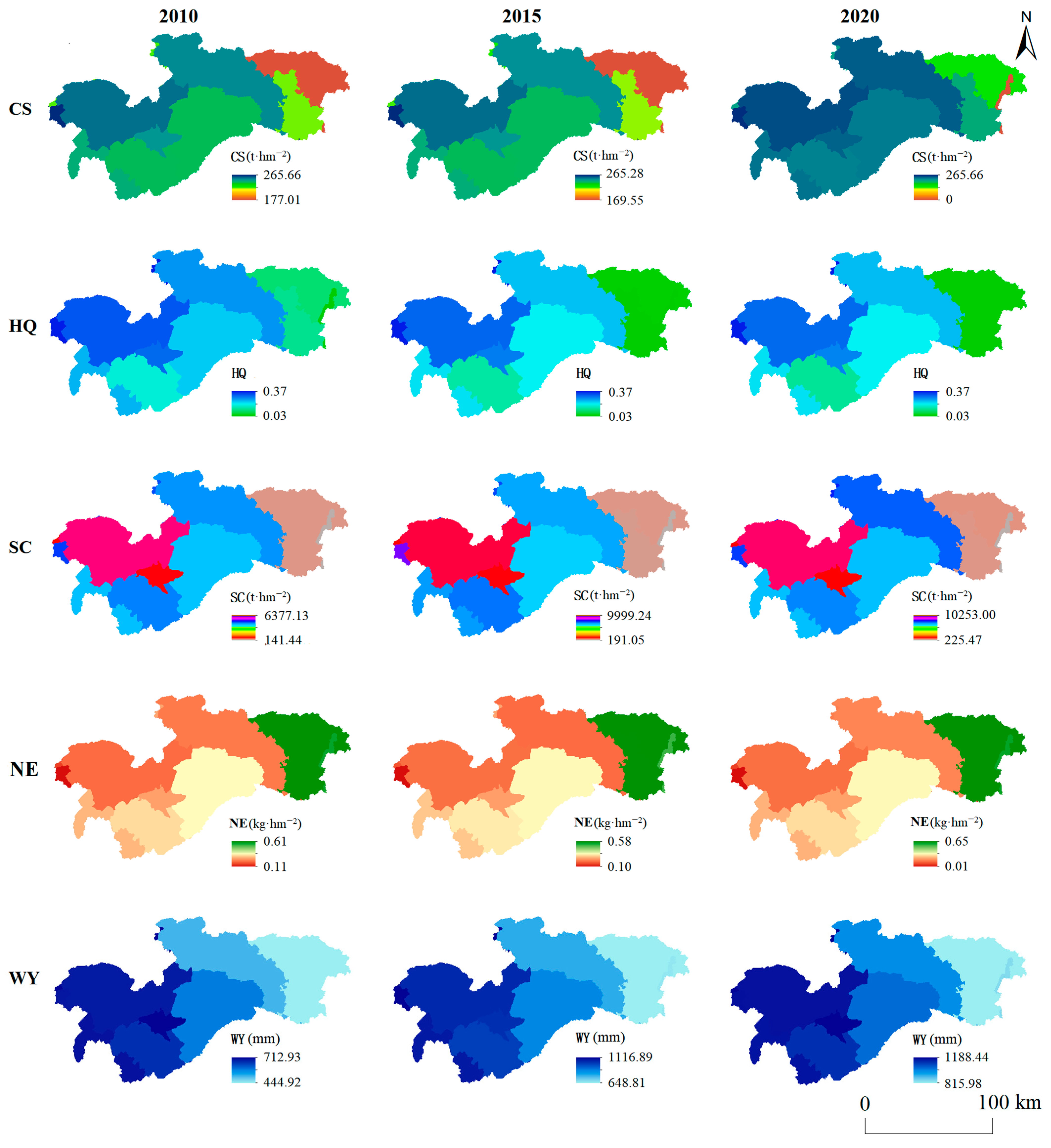
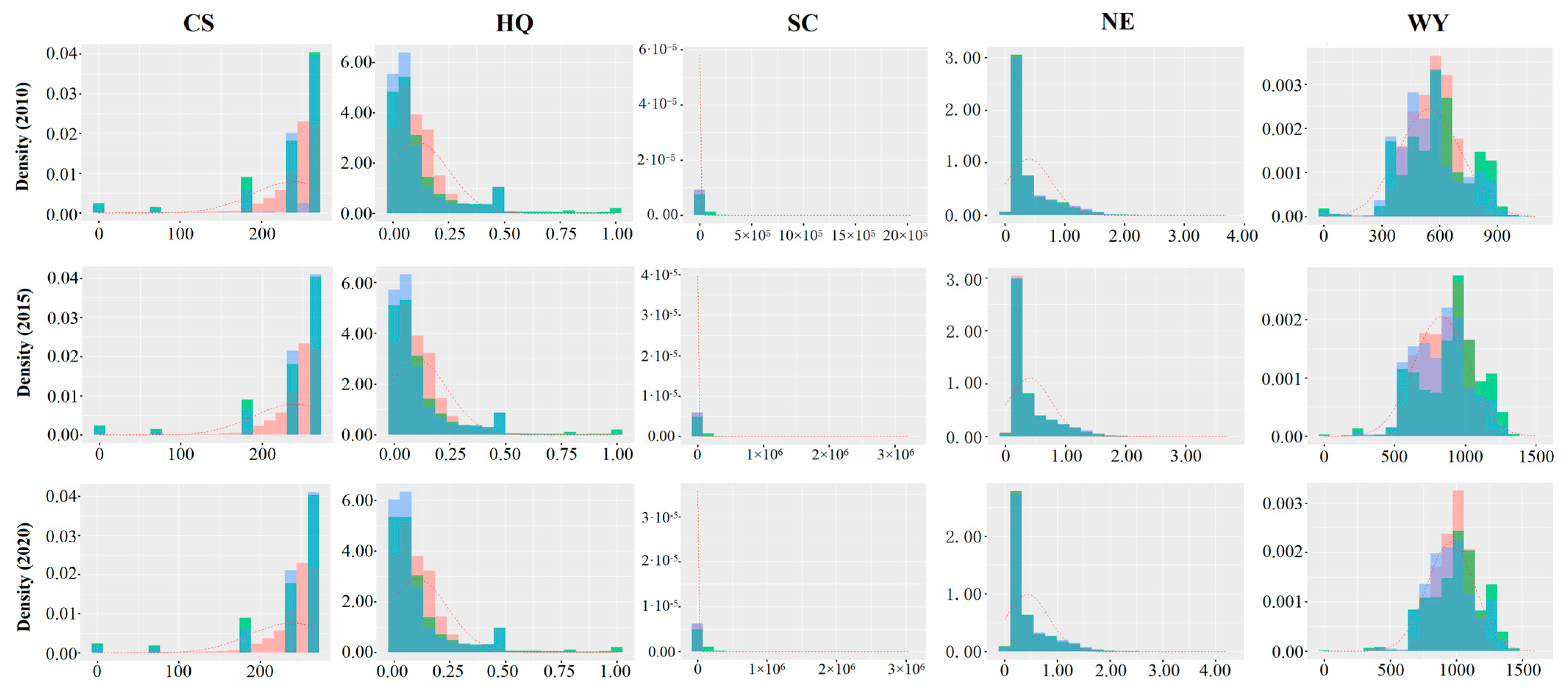
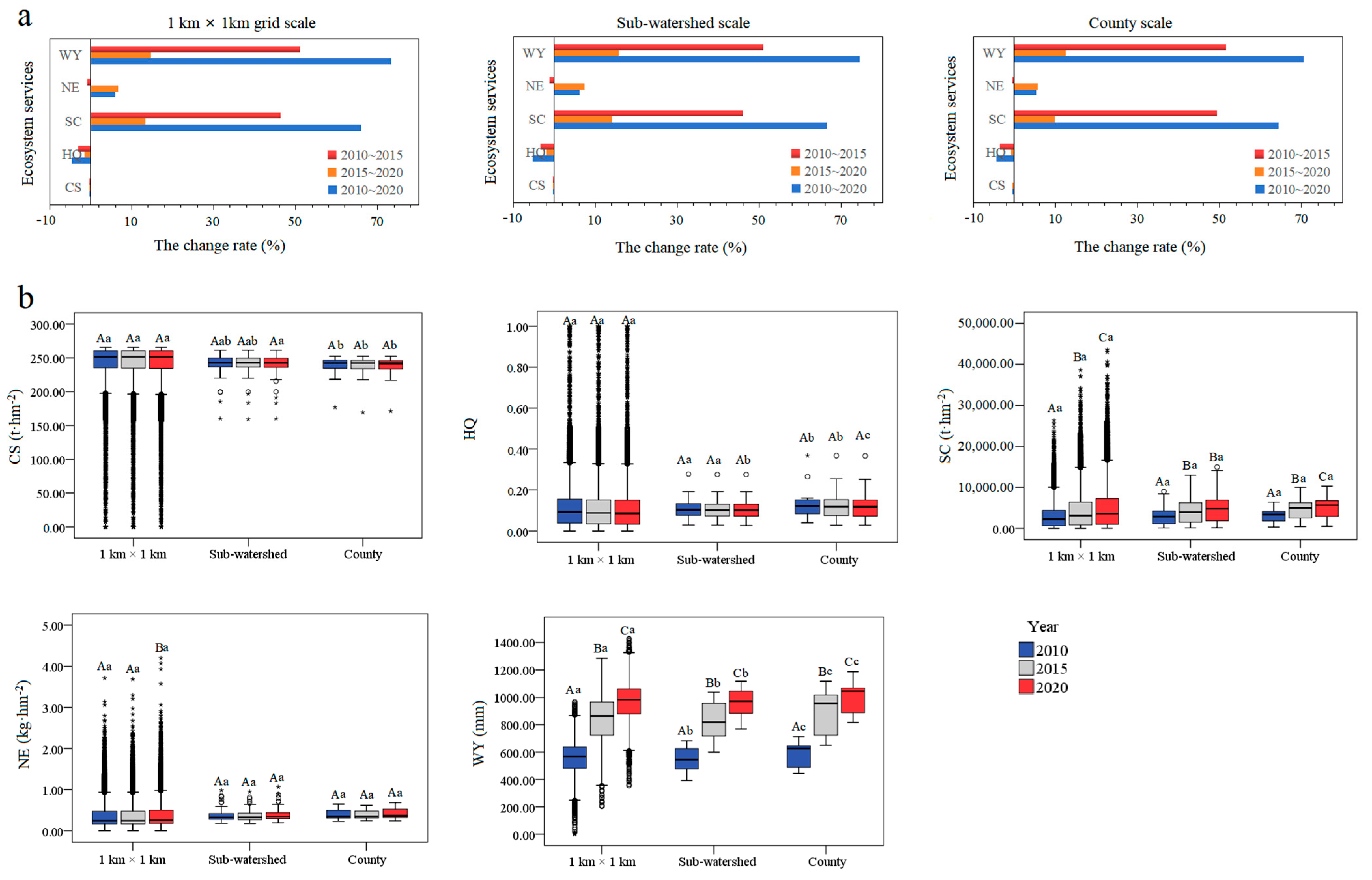
3.1. Spatiotemporal Distribution Characteristics of ESs

The provision of ESs in the Lishui River Basin exhibited evident spatial heterogeneity, while spatial distribution remained stable across different spatial (grid scale, sub-watershed scale, and county scale) and temporal scales (2010, 2015, and 2020) (Figure 3, Figure 4 and Figure 5). The overall values of ESs were to increase over time and with larger spatial scales, although there were certain variations in the temporal and spatial changes of individual ESs (Figure 6 and Figure 7).

From a temporal perspective, the change rate of ESs was consistent at three spatial scales (Figure 7a). Specifically, at the same spatial scale, average CS and HQ values saw a decline during the period of 2010–2020. In contrast, the supplies of SC, NE, and WY were enhanced. Initially, the average value of NE saw a slight dip from 2010 (0.37 kg/hm²) to 2015 (0.36 kg/hm²), followed by an increase up to 2020 (0.39 kg/hm²). Conversely, SC (3028.23–5023.75 t/hm²) and WY (558.79–969.56 mm) exhibited more significant change, with significant increases in their average values from 2010 to 2020, at an average change rate of 65.80%, 73.24%, respectively (p < 0.05, Figure 7b).

From a spatial perspective, comparing the spatial patterns of LULC (Figure 1) revealed that the spatial distribution of ESs across three scales (Figure 3, Figure 4 and Figure 5) was closely linked to LULC. Among them, the high-value areas of CS, HQ, and SC were predominantly found in the mountainous and hilly regions of the north and west. In contrast, the low-value areas were primarily located in the construction and cultivated lands of the east. Conversely, in NE, the high-value area was situated in the east and near water bodies of the basin, while the low-value area primarily extended across the northern and western regions. The WY exhibited a declining trend, moving from west to east. Moreover, the average ESs increased with increases in scale, reaching their highest values at the county level, with the exception of CS (Figure 7b). Among them, there were significant differences in CS between the county scale (234.51 t/hm²) and grid-scale (240.98 t/hm²). The HQ values were significantly larger at the county scale (0.14) than at other scales (0.11). WY exhibited significant differences across different scales, at an average of 792.54 mm, 779.13 mm, and 825.13 mm, respectively (p < 0.05).

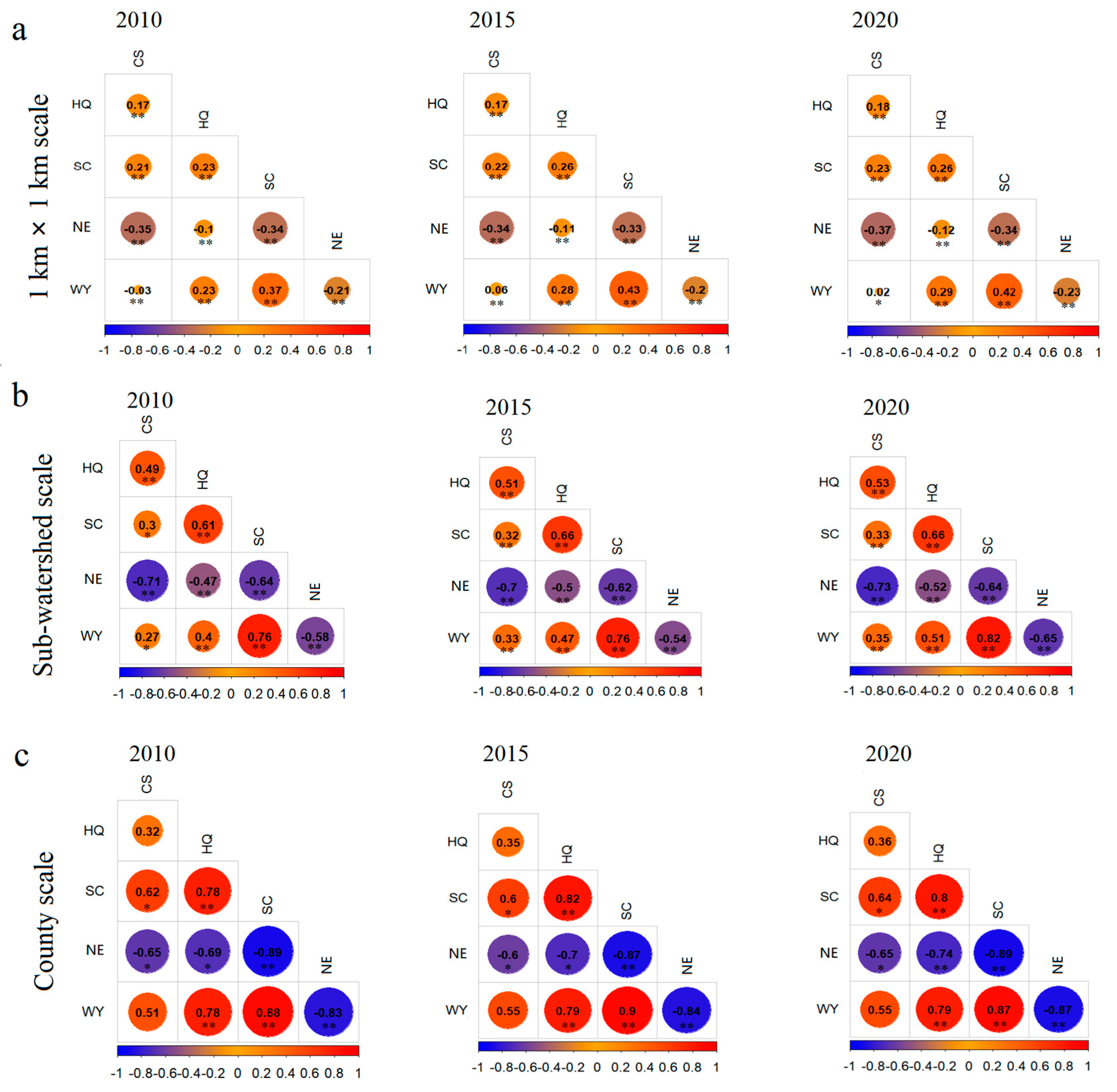
3.2. The Trade-Offs/Synergies Between ES Pairs

As depicted in Figure 8, ten ES pairings were identified among five ESs at three spatial scales within the Lishui River Basin, with the majority of these correlations proving statistically significant (p < 0.05). The dynamics between the same ES pair were consistent over the three years (except the CS-WY in 2010), and trade-offs/synergies of most ES pairs intensified as spatial scale increased. Spatially, there were six positive correlations involving CS, HQ, SC, and WY at most scales. In contrast, four NE-related ES pairs exhibited negative correlations, and these correlations increased as the scale expanded. Furthermore, the SC-WY pair demonstrated the greatest synergy across the three spatial scales, while the most significant trade-offs varied by scale: at the grid and sub-watershed scales, the CS-NE pair exhibited the largest trade-off; at the county scale, the SC-NE pair exhibited the largest trade-off.

From the perspective of temporal scale, the correlations of ESs pair presented similarly at the same scale from 2010 to 2020. Firstly, from 2010 to 2020, the absolute values of the correlation coefficients were the highest and lowest at the county scale and grid scale, respectively. Secondly, the tradeoffs and synergies among ESs remained consistent across different years. The absolute values of the correlation coefficients of most ES pairs were increased slightly from 2010 to 2020, with only the interaction direction between CS and WY changed.

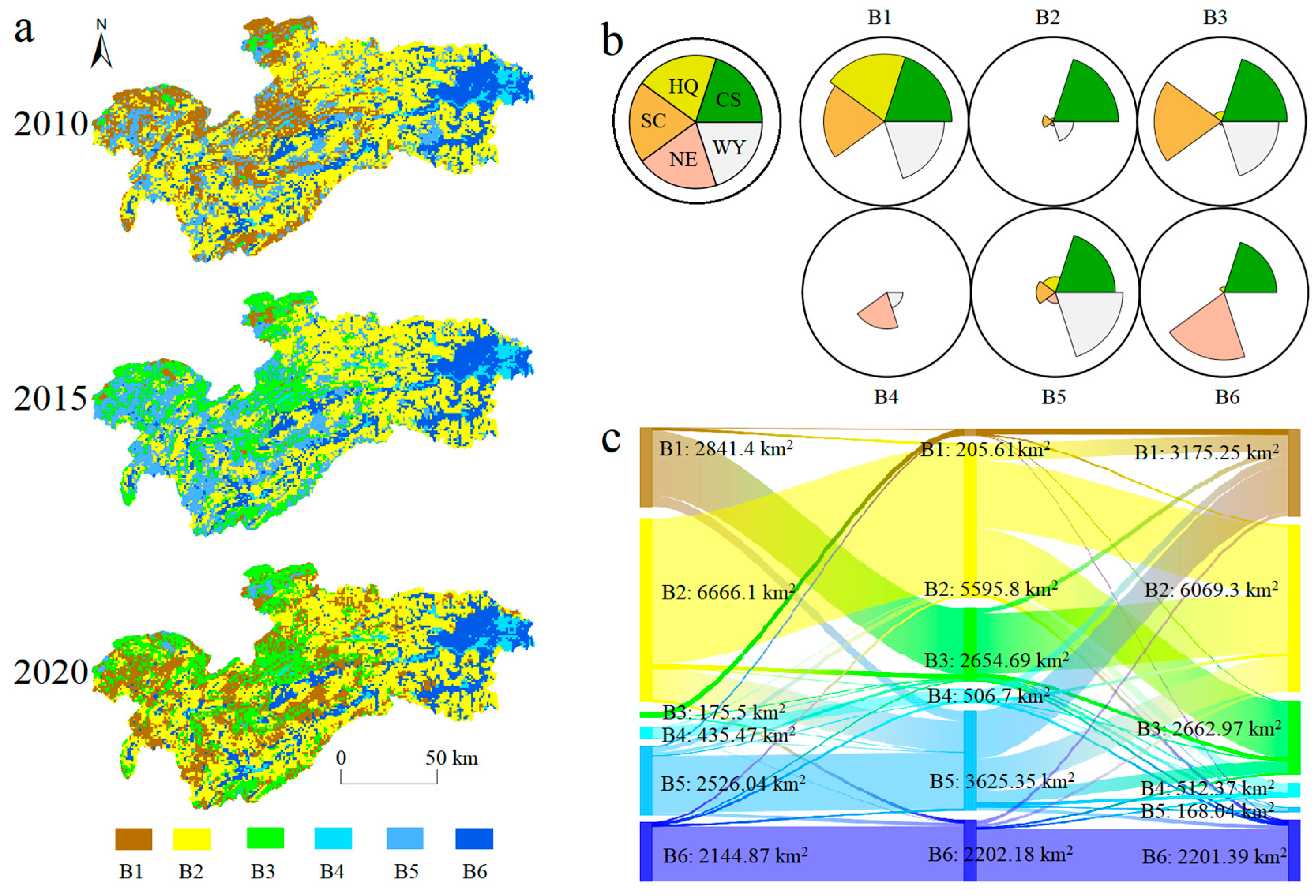
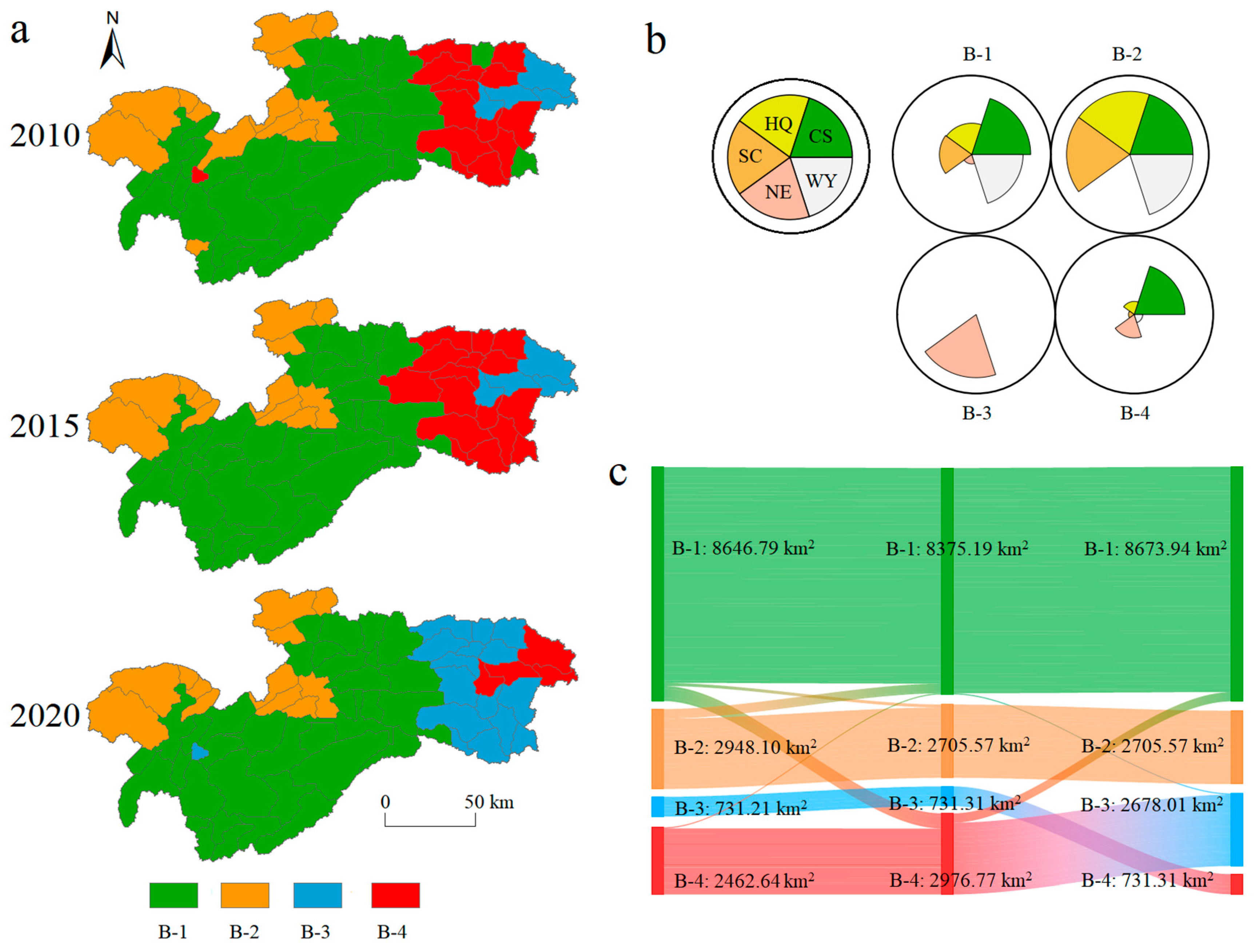
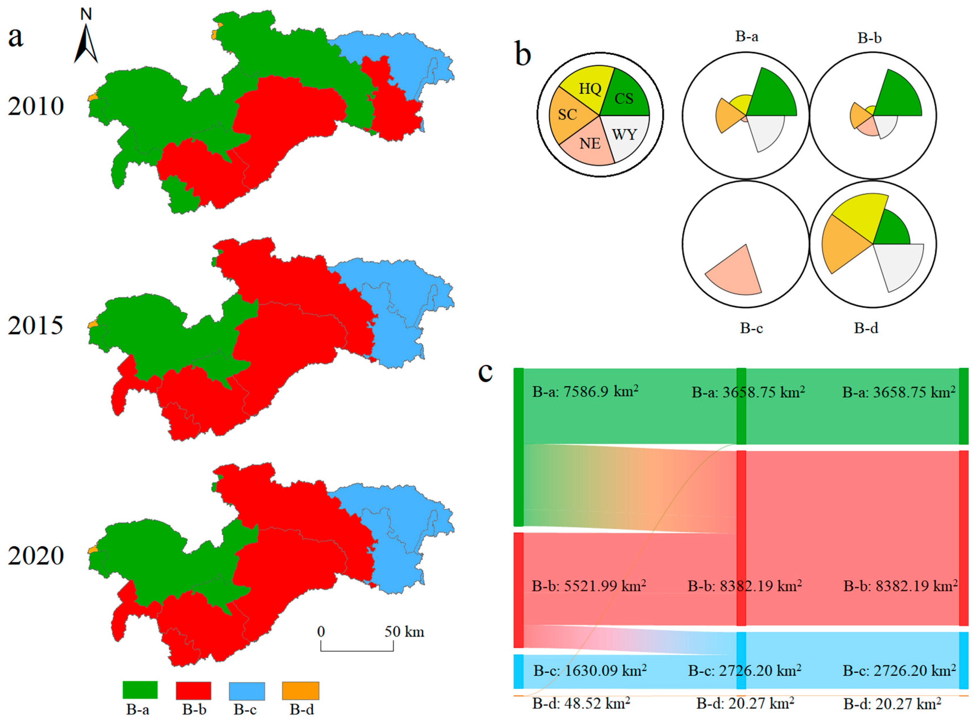
3.3. Spatial–Temporal Patterns of ES Bundles at Different Scales

The SOM analysis identified six ES bundles at the grid scale, four at the sub-watershed scale, and four at the county scale, as depicted in Figure 9, Figure 10 and Figure 11, respectively. The spatial distribution of ESBs showed variation over time. The patterns were relatively similar at two small scales, while the spatial pattern and internal structure of ESBs showed significant differentiation at the county scale. From 2010 to 2020, the transitions among different ESBs were most frequent at the grid scale, while it was relatively stable at other scales. Detailed characteristics of these ESBs are provided in the Supplementary Materials.

As shown in Figure 9, at the grid scale, the transitions of ESBs were frequent every 5 years, and B2 always dominates in different periods. Between 2010 and 2015, the areas of B3, B4, B5, and B6 exhibited an expansion, whereas the areas of B1 and B2 experienced a decline. In this stage, the transition from B1 to B3 was the most prominent, and the transition area between the two ESBs was the largest. From 2015 to 2020, the ESBs with expanded spatial distribution areas were B1, B2, B3, and B4, while the opposite was true for B5 and B6. The transformations of B5 to B1 and B5 to B2 were the most prominent during this period.

Figure 10 shows the transitions and spatio-temporal patterns of different bundles at the sub-watershed scale, where B-2 consistently dominates. From 2010 to 2015, there was an expansion in the area of B-4, whereas B-1 and B-2 declined, with B-3 maintaining stability. The most significant changes during this period included transitions from B-1 to B-4 and from B-2 to B-1. From 2015 to 2020, B-3 expanded while B-1 and B-4 contracted, with the most notable transitions occurring between B-3 and B-4.

As shown in Figure 11, at the county scale, B-a was dominant in spatial distribution in 2010, while B-b was dominant in other periods. Compared with the above two scales, there was less transformation between different ESBs from 2010 to 2020. From 2010 to 2015, the areas of bundles B-b and B-c expanded, whereas those of B-a and B-d contracted. During this time, notable transitions included the shift from B-a to B-b and from B-b to B-c. In contrast, the period from 2015 to 2020 saw no significant changes; the areas of all bundles remained relatively stable.

We observed that certain ES bundles exhibited similar spatial patterns across different scales. For instance, the key synergetic bundle and city bundle were consistent at two smaller scales, while the CS bundle was found at the grid and county scales. At the same time, the downstream city bundle was common to both the sub-watershed and county scales. Additionally, some ESBs were unique to specific scales: the CS-SC-WY synergy bundle was exclusive to the grid scale, and the HQ-SC-WY synergy bundle was specific to the county scale. The spatio-temporal differentiation of ESBs meant that differentiated approaches to ecosystem management need to be developed for target scales.

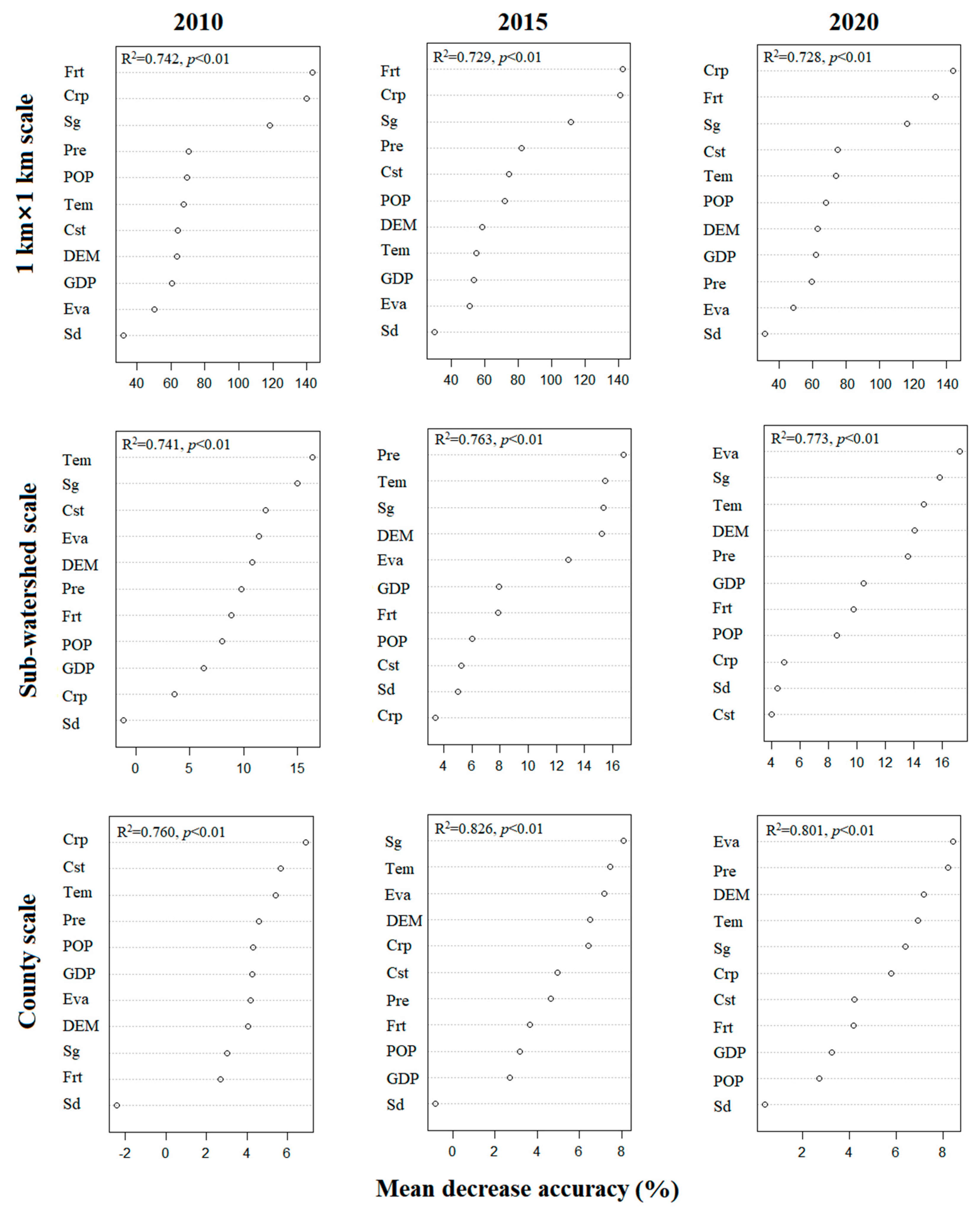
3.4. Social–Ecological Influences of ESs Bundles Distribution Across Different Times and Scales

As depicted in Figure 12, our results showed that Frt, Crp, and Sg were the most important factors influencing the spatial distribution of ESBs at the grid scale from 2010 to 2020, while the dominant factors changed with time at other scales. At the sub-watershed scale, Tem, Sg, and Cst were the primary drivers of ESB distribution in 2010. By 2015, Pre, Tem, and Sg had become the most significant drivers, while in 2020, Eva, Sg, and Tem took precedence. Overall, at the sub-watershed scale, ES bundles were consistently influenced by climatic factors (especially Tem) and Sg across all time periods. Similarly, at the county scale, Crp, Cst, and Tem were the key drivers of ESB distribution in 2010. By 2015, Sg, Tem, and Eva were most important, and in 2020, Eva, Pre, and DEM were the primary drivers. In general, the spatiotemporal distribution of ESBs at the county scale was driven by climate factors, land use factors, and topographic factors.

In summary, our analysis indicated that the main factors affecting the distribution of ESBs changed over time. At the grid scale, certain drivers consistently played a dominant role through the years. In contrast, key drivers at larger scales, such as sub-watersheds and counties, varied with time. Additionally, the mean decrease in accuracy in predicting the impact of these drivers tended to diminish as the scale increased. There were also variances in the ranking of dominant factors across different scales within the same year.

4. Discussion

4.1. Spatio-Temporal Characteristics of the Five ESs

The distribution of ESs demonstrates spatial heterogeneity and scale dependence, primarily depending on the varied spatial distribution of land use types, along with social and ecological factors, as noted in studies by Xu et al. [73] and Chen et al. [11]. Our research identified the areas with high values for CS, HQ, and SC were predominantly in the northern and western mountainous and hilly regions, which is similar to the findings of Wang et al. [74], mainly because the wide distribution of natural and semi-natural woodlands within the basin provides high carbon sinks, soil and water conservation capabilities, and intact habitats [75]. Our study found that WY showed a decreasing trend from west to east; this result was supported by Yang et al. [76] and Liao et al. [63]. This phenomenon can be attributed to the complex terrain, abundant rainfall, rich water resources, and effective vegetation protection measures in the area [42]. For example, the high and steep topographic features of mountain slopes can raise moist air currents, resulting in abundant precipitation and lower evapotranspiration, thus contributing to higher water supply capacity and ecological conservation potential in these areas [12]. Moreover, our study also investigated how ESs change over scales and time. ESs basically increased with the increase in scale (except CS), and the mean ESs were the largest at the county scale, which is similar to the existing studies [11]. These phenomena may be due to the variation in the composition of LULC types with spatial scale, thereby affecting the spatial pattern and mean values of ESs. However, CS and HQ were found to decrease over time at all three scales, suggesting that these ES types, which are highly correlated with biodiversity, tend to decline, which is easily overlooked in the study of a single time gradient. Therefore, it is necessary to analyze ESs at different time stages and spatial scales to find ESs with functional degradation and make them a priority type for ES management.

4.2. The Scale Effect of Trade-Offs and Synergies Among ESs

Existing studies highlight the importance of understanding the complex interactions of ESs for improving ecosystem management [5]. We observed that the interactions of ESs were predominantly synergistic across three scales, which is consistent with previous research [12,15,16]. Nonetheless, the scale of observation has a significant impact on the intensity of trade-offs and synergies among ESs, as indicated in studies by Han et al. [30], Sun et al. [49], and Pei et al. [77]. First, we discovered that the trade-offs and synergies strengthen among ESs with increasing scale. Our finding is similar to previous studies [12,15,49,77,78]. These variations in interaction intensity across scales highlight the complexity of ES interactions. As previous studies have pointed out, the observed results can be attributed to multiple reasons. One explanation involves the multi-scale effects of ecological processes, where the biophysical connections underlying ESs play different roles at different scales [79]. Another factor is that, at finer scales, there is less variation in the composition and configuration of LULC. However, when it is aggregated from grid to county scale, the composition of LULC increases, potentially transforming or intensifying the interaction between certain ESs [80]. Additionally, the larger the scale of the study, the richer the biodiversity, which may lead to improved resource use efficiency and, ultimately, an increased supply of ESs. This phenomenon is based on the niche complementarity effect and helps explain the scale effects observed in ES relationships [81]. Second, shifting scales did not alter the direction of interactions among ES pairs. This observation is consistent with the results of Qiao et al. [82], which demonstrated that the direction of ES interactions remains robust across different scales. However, Han et al. [30] found the different directions of ES interactions identified at the grid, watershed, and township scales; this differs from the findings of our study, where the direction of the ES interactions remains consistent across different scales. This may be due to the significant role natural factors play in shaping ES tradeoffs and synergies. Additionally, the diversity of landform types across different counties and basins, along with factors like altitude, soil, and climate, may increase the complexity and variability of ES relationships. Therefore, studying ES interactions in various geographical regions must consider scale effects in relation to specific environmental contexts. This approach provides valuable guidance for managing ecosystems and for sustainable spatial planning across different scales [83].

4.3. Historical Patterns and Dynamics of ESBs Across Various Scales and Their Socio-Ecological Drivers

In order to effectively manage multiple ESs simultaneously, ESBs formed by the spatial aggregation of multiple ESs can be identified [10,19,75]. Unlike previous studies [12,17,84], our research did not limit bundle division to the fine grid scale. Instead, we also incorporated the sub-watershed and county scales. This approach revealed more pronounced spatial–temporal heterogeneity of ESBs and highlighted greater differences in their spatial distribution across various scales. Specifically, at the grid scale, B1 (key synergistic bundle) in the northern and western parts of the study area exhibited high ES diversity. This region is characterized by a high supply of most ESs, strong synergy among ESs, complex edge shapes, and a high degree of fragmentation in spatial distribution. This observation aligns with the findings of Dong et al. [84], which suggested that the significant differences in the natural environment between regions lead to variations in the degree of aggregation of ESBs. However, we found that the spatial distribution of ESBs at the county scale was more different than that at the other two scales, mainly because the distribution of ESBs at smaller scales is more robust [7]. It was worth noting that the eastern region of our study area was identified as a downstream city bundle or city bundle at three scales, and the proportion in the study area continues to expand. These findings are consistent with the research results of Xia et al. [12], Feng et al. [18], and Yan et al. [67]. They also described the evolution trajectory of the ESBs similar to the city bundle, which is mainly related to vegetation degradation caused by urban expansion [18]. Furthermore, those clusters are located in a flat area with frequent human activities and a considerable distribution of water bodies, farmlands, and construction land. The provision capacity of various services (except NE) within the cluster is generally low. However, because of the high proportion of built-up land, the nutrient retention efficiency is relatively low. The high runoff coefficient increases the transfer of water and nutrients, resulting in relatively high NE capabilities [85]. Nevertheless, the high nutrient output poses a pollution risk to the water quality downstream of the watershed. This indicated that the region where such bundles were located is mainly an ES demand area and also a priority management area, and it is necessary to comprehensively consider the enhancement of multiple ESs and their synergistic effects. In the future, it is essential to follow the principle of “prioritizing ecological protection while supporting urban development” to ensure clear separation between regional development zones and ecological protection red lines, avoiding any intersection or conflict.

Our research indicated that the factors influencing the spatial distribution of ESB vary with time and scale. Generally, in large-scale studies, climate characteristics, geomorphic features, and urbanization are the primary drivers of ES changes [68,86]. Conversely, at smaller scales, land use patterns and management practices [87] are the main influencing factors that align with our findings. For instance, at the grid scale, the spatial distribution of ESBs was predominantly influenced by LULC (Frt, Crp), consistent with numerous existing studies [84,88,89]. This is because different ESBs are associated with varying land use structures, and their spatial and temporal changes are closely linked to these land use types [84]. However, some studies [67] have found that natural factors such as DEM and normalized vegetation index have a decisive impact on the spatial distribution and evolution of ESBs. This contrasts with our findings, where drivers vary by scale, primarily due to the different methods used. Our study primarily combines Pearson correlation analysis, SOM, and random forest models to provide a new perspective on the cross-scale interactions of ES and their driving factors. Therefore, future research should consider how research methods affect the results. At the sub-watershed scale, Tem and Sg were the main factors influencing ESBs’ spatiotemporal distribution, while climate and topography were dominant at the county scale. Notably, Sg had a more significant impact on ESBs’ spatiotemporal heterogeneity than DEM and Sd. Similar conclusions are drawn by Dong et al. [84] and Wang et al. [90]. This may be because urban expansion extends human activities to higher altitudes, where steep slopes provide greater resistance to such activities [91], limiting their extent and promoting vegetation growth [92]. Additionally, topography factors influence distinct ecological patterns by modifying the spatial distribution of natural and human settlements [93], thereby affecting ESBs’ spatial distribution. Climatic factors significantly influence ES interactions and ecosystem functions by participating in various biogeochemical processes. In summary, the primary drivers of ESBs exhibited spatiotemporal scale effects, meaning socio-ecological drivers critical at one scale may not be as influential at another. Therefore, considering the scale-dependent nature of the dynamics distribution drivers of ESBs, it is essential to formulate distinct sustainable ecosystem management strategies that are specifically adapted to each scale.

4.4. Limitations and Prospects

This study provides scientific analytical methods and theoretical guidance for the sustainable and hierarchical management of ESs in medium-scale watersheds. However, there are limitations. First, the types of ESs investigated are limited. MEA categorizes ESs into four main types: provisioning, regulating, supporting, and cultural services. Our study only evaluated five Ess, namely CS, HQ, NE, SC, and WY, none of which involve cultural services. The limited types of ESs might not adequately reflect the spatial–temporal variation trends of ESs. Second, there are limitations to the study scale. Although this study has more scale categories (1 km × 1 km grid, sub-watershed, and county) compared to other studies, the limited scales might lead to inaccurate results when exploring the scale effects of interactions between ESs. Future studies should incorporate finer scales to accurately investigate the critical turning points of the “scale effect,” enhancing the applicability of ES management strategies. Third, the limitations of the model application: This study only uses the InVEST model to quantify the supply of ESs. Currently, numerous ecological models are emerging, and different models may yield significantly different assessment results for the same area. Future research should apply both the InVEST and SWAT ecological models to evaluate the same services for comparison. By comparing different assessment methods, the best ecological model can be selected, improving the accuracy of the study results.

5. Conclusions

To gain a more detailed understanding of the interactions among ESs and their spatiotemporal co-occurrence, we investigated the spatio-temporal characteristics, scale effects, and driving mechanisms of ES interactions in the Lishui River Basin across three scales. Several key findings emerged: (1) The spatial distribution of ESs exhibited heterogeneity; the ESs value was larger in the western mountainous and hilly areas. Moreover, SC and WY significantly improved, while CS and HQ showed a declining trend from 2010 to 2020. This indicates that forests are crucial for providing ESs in the basin, yet recent declines in CS and HQ underscore the need for better management and protection of natural resources. (2) The trade-off and synergistic relationships of ESs remain relatively stable over time. However, the intensity of these relationships increased with the expansion of spatial scales, indicating that the interaction of ESs exhibits scale heterogeneity. (3) Over time and spatial scales, the distribution of ESBs and their socio-ecological drivers changed, with a notable expansion of city and downstream city bundles. The ESB flows and transformations were most frequent at the grid scale, with spatial differences increasing with scale. The LULC was the key factor affecting ESB patterns at the grid scale, while at larger scales, climate and topography were dominant, indicating varying ES management priorities across scales. This knowledge offers crucial insights for regional hierarchical management and fostering the sustainable development of the social economy.

References

1. Jiang, C.; Zhang, H.; Zhang, Z. Spatially explicit assessment of ecosystem services in China’s Loess Plateau: Patterns, interactions, drivers, and implications. Glob. Planet. Change 2018, 161, 41–52. [Google Scholar]
2. Costanza, R.; d’Arge, R.; de Groot, R.; Farber, S.; Grasso, M.; Hannon, B.; Limburg, K.; Naeem, S.; O’Neill, R.V.; Paruelo, J.; et al. The value of the world’s ecosystem services and natural capital. Nature 1997, 387, 253–260. [Google Scholar]
3. Feng, Q.; Zhao, W.; Fu, B.; Ding, J.; Wang, S. Ecosystem service trade-offs and their influencing factors: A case study in the Loess Plateau of China. Sci. Total Environ. 2017, 607–608, 1250–1263. [Google Scholar]
4. Wu, J.G. Effects of changing scale on landscape pattern analysis: Scaling relations. Landsc. Ecol. 2004, 19, 125–138. [Google Scholar] [CrossRef]
5. Raudsepp-Hearne, C.; Peterson, G.D.; Bennett, E.M. Ecosystem service bundles for analyzing tradeoffs in diverse landscapes. Proc. Natl. Acad. Sci. USA 2010, 107, 5242–5247. [Google Scholar] [CrossRef]
6. Gao, J.; Zuo, L. Revealing ecosystem services relationships and their driving factors for five basins of Beijing. J. Geogr. Sci. 2021, 31, 111–129. [Google Scholar] [CrossRef]
7. Raudsepp-Hearne, C.; Peterson, G.D. Scale and ecosystem services: How do observation, management, and analysis shift with scale—Lessons from Québec. Ecol. Soc. 2016, 21, 16. [Google Scholar]
8. Cord, A.F.; Bartkowski, B.; Beckmann, M.; Dittrich, A.; Hermans-Neumann, K.; Kaim, A.; Lienhoop, N.; Locher-Krause, K.; Priess, J.; Schröter-Schlaack, C.; et al. Towards systematic analyses of ecosystem service trade-offs and synergies: Main concepts, methods and the road ahead. Ecosyst. Serv. 2017, 28, 264–272. [Google Scholar] [CrossRef]
9. Qiu, J.; Turner, M.G. Spatial interactions among ecosystem services in an urbanizing agricultural watershed. Proc. Natl. Acad. Sci. USA 2013, 110, 12149–12154. [Google Scholar]
10. Spake, R.; Lasseur, R.; Crouzat, E.; Bullock, J.M.; Lavorel, S.; Parks, K.E.; Schaafsma, M.; Bennett, E.M.; Maes, J.; Mulligan, M.; et al. Unpacking ecosystem service bundles: Towards predictive mapping of synergies and trade-offs between ecosystem services. Glob. Environ. Chang. 2017, 47, 37–50. [Google Scholar]
11. Chen, J.C.; He, S.Y.; Xue, J.; Zhang, H.Y.; Li, Z.H.; Wang, L.; Li, K. Exploring ecosystem service trade-offs and their response to landscape configuration at multi-scales: A case study of Hubei Province. Acta Ecol. Sin. 2023, 43, 4835–4846. (In Chinese) [Google Scholar]
12. Xia, G.; Yuan, S.F.; Alexander, V.; Prishchepov, A.V. Spatial-temporal heterogeneity of ecosystem service interactions and their social-ecological drivers: Implications for spatial planning and management. Resour. Conserv. Recycl. 2023, 189, 106767. [Google Scholar]
13. Karimi, J.D.; Corstanje, R.; Harris, J.A. Understanding the importance of landscape configuration on ecosystem service bundles at a high resolution in urban landscapes in the UK. Landsc. Ecol. 2021, 36, 2007–2024. [Google Scholar]
14. Li, T.; Liang, X.Y.; Zhang, J.; Geng, Y.; Geng, T.W.; Shi, J.X. Ecosystem service trade-off and synergy relationship and its driving factor analysis based on Bayesian belief network: A case study of the Loess Plateau in northern Shanxi Province. Acta Ecol. Sin. 2023, 43, 6758–6771. (In Chinese) [Google Scholar]
15. Zheng, D.; Wang, Y.; Hao, S.; Xu, W.; Lv, L.; Yu, S. Spatial-temporal variation and tradeoffs/synergies analysis on multiple ecosystem services: A case study in the Three-River Headwaters region of China. Ecol. Indic. 2020, 116, 106494. [Google Scholar]
16. Yang, G.; Ge, Y.; Xue, H.; Yang, W.; Shi, Y.; Peng, C.; Du, Y.; Fan, X.; Ren, Y.; Chang, J. Using ecosystem service bundles to detect tradeoffs and synergies across urban–rural complexes. Landsc. Urban Plan. 2015, 136, 110–121. [Google Scholar] [CrossRef]
17. Gou, M.M.; Li, L.; Ouyang, S.; Wang, N.; La, L.M.; Liu, C.F.; Xiao, W.F. Identifying and analyzing ecosystem service bundles and their socioecological drivers in the Three Gorges Reservoir Area. J. Clean. Prod. 2021, 307, 127208. [Google Scholar]
18. Feng, Z.; Peng, J.; Wu, J.S. Ecosystem service bundles based approach to exploring the trajectories of ecosystem service spatiotemporal change: A case study of Shenzhen City. Acta Ecol. Sin. 2020, 40, 2545–2554. (In Chinese) [Google Scholar]
19. Quintas-Soriano, C.; García-Llorente, M.; Norstrm, A.; Meacham, M.; Castro, A.J. Integrating supply and demand in ecosystem service bundles characterization across Mediterranean transformed landscapes. Landsc. Ecol. 2019, 34, 1619–1633. [Google Scholar]
20. Li, H.L.; Peng, J.; Hu, Y.N.; Wu, W.H. Ecological function zoning in Inner Mongolia Autonomous Region based on ecosystem service bundles. Chin. J. Appl. Ecol. 2017, 28, 2657–2666. (In Chinese) [Google Scholar]
21. Shen, J.S.; Liang, Z.; Liu, L.B.; Li, D.L.; Zhang, Y.T.; Li, S.C. Trade-offs and synergies of ecosystem service bundles in Xiong’an New Area. Geogr. Res. 2020, 39, 79–91. (In Chinese) [Google Scholar]
22. Dou, H.S.; Li, X.B.; Li, S.K.; Dang, D.L.; Li, X.; Liu, X.; Li, M.Y.; Liu, S.Y. Mapping ecosystem services bundles for analyzing spatial trade-offs in inner Mongolia. J. Clean. Prod. 2020, 256, 120444. [Google Scholar] [CrossRef]
23. Shen, J.; Li, S.; Liu, L.; Liang, Z.; Wang, Y.; Wang, H.; Wu, S. Uncovering the relationships between ecosystem services and social-ecological drivers at different spatial scales in the Beijing-Tianjin-Hebei region. J. Clean. Prod. 2021, 290, 125193. [Google Scholar]
24. Renard, D.; Rhemtulla, J.M.; Bennett, E.M. Historical dynamics in ecosystem service bundles. Proc. Natl. Acad. Sci. USA 2015, 112, 13411–13416. [Google Scholar] [CrossRef]
25. Meacham, M.; Queiroz, C.; Norström, A.V.; Peterson, G.D. Social-ecological drivers of multiple ecosystem services: What variables explain patterns of ecosystem services across the Norrström drainage basin? Ecol. Soc. 2016, 21, 14. [Google Scholar]
26. Dade, M.C.; Mitchell, M.G.; McAlpine, C.A.; Rhodes, J.R. Assessing ecosystem service trade-offs and synergies: The need for a more mechanistic approach. Ambio 2019, 48, 1116–1128. [Google Scholar]
27. Sun, X.; Tang, H.; Yang, P.; Hu, G.; Liu, Z.; Wu, J. Spatiotemporal patterns and drivers of ecosystem service supply and demand across the conterminous United States: A multiscale analysis. Sci. Total Environ. 2020, 703, 135005. [Google Scholar]
28. Goldstein, J.H.; Caldarone, G.; Duarte, T.K.; Ennaanay, D. Integrating ecosystem-service tradeoffs into land-use decisions. Proc. Natl. Acad. Sci. USA 2012, 109, 7565–7570. [Google Scholar]
29. Vallet, A.; Locatelli, B.; Levrel, H.; Wunder, S.; Seppelt, R.; Scholes, R.J.; Oszwald, J. Relationships between ecosystem services: Comparing methods for assessing tradeoffs and synergies. Ecol. Econ. 2018, 150, 96–106. [Google Scholar]
30. Han, X.J.; Wang, J.J.; Wen, X. The scale effect and differentiation mechanism of the relationship between ecosystem services in the grain for green area: A case study of Ansai District. Acta Ecol. Sin. 2024, 44, 1791–1807. (In Chinese) [Google Scholar]
31. Tomscha, S.A.; Sutherland, I.J.; Renard, D.; Gergel, S.E.; Rhemtulla, J.M.; Bennett, E.M.; Daniels, L.D.; Eddy, I.M.; Clark, E.E. A guide to historical data sets for reconstructing ecosystem service change over time. BioScience 2016, 66, 747–762. [Google Scholar] [CrossRef]
32. Zhu, C.; Dong, B.; Li, S.; Lin, Y.; Shahtahmassebi, A.; You, S.; Zhang, J.; Gan, M.; Yang, L.; Wang, K. Identifying the trade-offs and synergies among land use functions and their influencing factors from a geospatial perspective: A case study in Hangzhou. J. Clean. Prod. 2021, 314, 128026. [Google Scholar]
33. Hou, Y.; Lu, Y.H.; Chen, W.P.; Fu, B.J. Temporal variation and spatial scale dependency of ecosystem service interactions: A case study on the central Loess Plateau of China. Landsc. Ecol. 2017, 32, 1201–1217. [Google Scholar]
34. Schirpke, U.; Candiago, S.; Egarter Vigl, L.; Jäger, H.; Labadini, A.; Marsoner, T.; Meisch, C.; Tasser, E.; Tappeiner, U. Integrating supply, flow and demand to enhance the understanding of interactions among multiple ecosystem services. Sci. Total Environ. 2019, 651, 928–941. [Google Scholar] [CrossRef]
35. Lautenbach, S.; Kugel, C.; Lausch, A.; Seppelt, R. Analysis of historic changes in regional ecosystem service provisioning using land use data. Ecol. Indic. 2011, 11, 676–687. [Google Scholar]
36. Zhang, Z.; Liu, Y.; Wang, Y.; Liu, Y.; Zhang, Y.; Zhang, Y. What factors affect the synergy and tradeoff between ecosystem services, and how, from a geospatial perspective? J. Clean. Prod. 2020, 257, 120454. [Google Scholar]
37. Feng, Z.; Jin, X.; Chen, T.; Wu, J. Understanding trade-offs and synergies of ecosystem services to support the decision-making in the Beijing–Tianjin–Hebei region. Land Use Policy 2021, 106, 105446. [Google Scholar] [CrossRef]
38. Hamann, M.; Biggs, R.; Reyers, B. Mapping social-ecological systems: Identifying ‘green-loop’ and ‘red-loop’ dynamics based on characteristic bundles of ecosystem service use. Glob. Environ. Chang. 2015, 34, 218–226. [Google Scholar]
39. O’Higgins, T.; Nogueira, A.A.; LillebøA, I.; O’Higgins, T.; Nogueira, A.A.; Lillebøa, I. A simple spatial typology for assessment of complex coastal ecosystem services across multiple scales. Sci. Total Environ. 2019, 649, 1452–1466. [Google Scholar] [CrossRef]
40. Sun, X.; Wu, J.; Tang, H.; Yang, P. An urban hierarchy-based approach integrating ecosystem services into multiscale sustainable land use planning: The case of China. Resour. Conserv. Recycl. 2022, 178, 106097. [Google Scholar]
41. Liu, B.W.; Song, N.; Geng, S.H.; Chen, Q. Evolution characteristics and impacting factors of annual runoff and sediment in Lishui River during 1955–2009. Bull Soil Water Conserv. 2014, 34, 360–363. (In Chinese) [Google Scholar]
42. Guo, R.Z.; Shen, H.J.; Yang, M.H. Studies on ecosystem service value and ecological compensation strategy in Lishui River Basin. Res. Environ. Sci. 2016, 29, 774–782. [Google Scholar]
43. Sun, Z.; Lotz, T.; Chang, N.B. Assessing the long-term effects of land use changes on runoff patterns and food production in a large lake watershed with policy implications. J. Environ. Manag. 2017, 204, 92–101. [Google Scholar] [CrossRef]
44. Zeng, Z.W.; Yang, H.; Ning, Q.M.; Tang, H. Temporal and spatial evolution of land use intensity and its impact on ecosystem services in Dongting Lake Zone. Econ. Geogr. 2022, 42, 176–185. [Google Scholar]
45. Turner, M.G.; Donato, D.C.; Romme, W.H. Consequences of spatial heterogeneity for ecosystem services in changing forest landscapes: Priorities for future research. Landsc. Ecol. 2013, 28, 1081–1097. [Google Scholar] [CrossRef]
46. Xu, X.L.; Zhuang, D.F.; Jia, S.F.; Hu, Y.F. Automatic extraction of drainages in China based on DEM in GIS environment. Resour. Environ. Yangtze Basin 2004, 13, 343–348. (In Chinese) [Google Scholar]
47. Millennium Ecosystem Assessment (MEA). Ecosystems and Human Well-Being: Synthesis; Island Press: Washington, DC, USA, 2005. [Google Scholar]
48. Sun, X.Y.; Shan, R.F.; Liu, F. Spatio-temporal quantification of patterns trade-offs and synergies among multiple hydrological ecosystem services in different topographic basins. J. Clean Prod. 2020, 268, 122338. [Google Scholar] [CrossRef]
49. Sun, Z.X.; Liu, Z.F.; He, C.Y.; Wu, J.G. Multi-scale analysis of ecosystem service trade-offs in urbanizing drylands of China: A case study in the Hohhot-Baotou-Ordos-Yulin region. Acta Ecol. Sin. 2016, 36, 4881–4891. (In Chinese) [Google Scholar]
50. Yang, J.; Zhou, P.Q.; Yuan, S.J.; Tan, X.; Lou, Z.F. Land Ecosystem Service Functions for Dongting Lake Ecological Economic Zone Based on InVEST Model. Bull Soil Water Conserv. 2022, 42, 267–272, 282. (In Chinese) [Google Scholar]
51. Fu, B.; Xu, P.; Wang, Y.K.; Peng, Y.; Ren, J. Spatial pattern of water retention in Dujiangyan County. Geosciences 2013, 48, 856–866. (In Chinese) [Google Scholar]
52. Zhang, X.; Zhang, G.; Long, X.; Zhang, Q.; Liu, D.; Wu, H.; Li, S. Identifying the drivers of water yield ecosystem service: A case study in the Yangtze River Basin, China. Ecol. Indic. 2021, 132, 108304. [Google Scholar] [CrossRef]
53. Guo, Y.; Li, P.; Cheng, W.J.; Xiao, Z.Y.; Mu, Y.L.; Zhi, L.H.; Li, X.W. Evaluation and complex relations analysis of ecosystem services based on spatial-temporal change of land use in Dongting Lake. Acta Sci. Circumstant. 2022, 42, 121–130. (In Chinese) [Google Scholar]
54. Williams, J.R. The erosion-productivity impact calculator (EPIC) model: A case history. Philos. Trans. R. Soc. Lond. B Biol. Sci. 1990, 329, 421–428. [Google Scholar]
55. Ouyang, L.Y. The Research on the Effects of LUCC on Ecosystem Services in Dongting Lake Region Based on InVEST Model; Central South University of Forestry and Technology: Hunan, China, 2022. (In Chinese) [Google Scholar]
56. Li, T.; Liu, K.; Hu, S.; Bao, Y.B. Soil erosion and ecological benefits evaluation of Qinling Mountains based on the InVEST model. Resour. Environ. Yangtze Basin 2014, 23, 1242–1250. (In Chinese) [Google Scholar]
57. Ouyang, Z.; Hua, Z.; Yang, X.; Polasky, S.; Daily, G.C. Improvements in ecosystem services from investments in natural capital. Science 2016, 352, 1455–1459. [Google Scholar] [CrossRef]
58. Sharp, R.; Tallis, H.T.; Ricketts, T.; Nelson, E.; Ennaanay, D.; Wolny, S.; Olwero, N.; Vigerstol, K.; Aukema, J.; Diedenhoven, M.; et al. InVEST User’s Guide; The Natural Capital Project: Stanford, CA, USA, 2014. [Google Scholar]
59. Xu, L.; He, N.; Yu, G. A dataset of carbon density in Chinese terrestrial ecosystems (2010s). China Sci. Data 2018, 3, 26. [Google Scholar] [CrossRef]
60. Fang, L.L.; Wang, L.C.; Chen, W.X.; Sun, J.; Cao, Q.; Wang, S.Q.; Wang, L. Identifying the impacts of natural and human factors on ecosystem service in the Yangtze and Yellow River Basins. J. Clean. Prod. 2021, 314, 127995. [Google Scholar] [CrossRef]
61. Liu, Y.; Zhou, Y.; Du, Y.T. Study on the Spatio-Temporal Patterns of Habitat Quality and Its Terrain Gradient Effects of the Middle of the Yangtze River Economic Belt Based on InVEST Model. Resour. Environ. Yangtze Basin 2019, 28, 2429–2440. (In Chinese) [Google Scholar]
62. Sharp, R.; Douglass, J.; Wolny, S.; Arkema, K.; Bermhardt, J.; Bierbower, W.; Cchaumont, N.; Denu, D.; Fisher, D.; Glowinski, K.; et al. InVEST 3.7.0 User’s Guide; Stanford University: Stanford, CA, USA; University of Minnesota: Minneapolis, MN, USA; The Nature Conservancy: Arlington County, VA, USA; World Wildlife Fund: Gland, Switzerland, 2018. [Google Scholar]
63. Liao, J.B.; Mao, D.H.; Deng, M.R. Evaluation of typical ecosystem services and trade-offs/synergies in Dongting Lake Basin. Resour. Environ. Yangtze Basin 2024, 33, 310–321. (In Chinese) [Google Scholar]
64. Jiang, W.; Fu, B.J.; Shu, Z.G.; Lv, Y.H.; Gao, G.Y.; Feng, X.M.; Schüler, S.; Wu, X.; Wang, C. Spatiotemporal drivers of Nature’s contributions to people: A county level study. Environ. Sci. Ecotechnol. 2024, 20, 100430. [Google Scholar] [CrossRef]
65. Chen, T.Q.; Feng, Z.; Zhao, H.F.; Wu, K.N. Identification of ecosystem service bundles and driving factors in Beijing and its surrounding areas. Sci. Total Environ. 2019, 711, 134687. [Google Scholar] [CrossRef]
66. Yang, S.W.; Liu, J.F.; Kuang, Y.W.; Wang, Q.; Huang, R.Z.; Nie, W.; Sun, J.Y.; Zhao, Y.P. Spatiotemporal dynamics and driving forces of ecosystem service trade-offs and synergies in Jiangxi Province. Chin. J. Ecol. 2023, 42, 1234–1245. (In Chinese) [Google Scholar]
67. Yan, X.L.; Li, X.Y.; Liu, C.H.; Li, J.W.; Zhong, J.Q. Spatial evolution trajectory of ecosystem service bundles and its social-ecological driven by geographical exploration: A case study of Dalian. Acta Ecol. Sin. 2022, 42, 5734–5747. (In Chinese) [Google Scholar]
68. Peng, J.; Tian, L.; Liu, Y.X.; Zhao, M.Y.; Hu, Y.N.; Wu, J.S. Ecosystem services response to urbanization in metropolitan areas: Thresholds identification. Sci. Total Environ. 2017, 607–608, 706–714. [Google Scholar] [CrossRef]
69. Breiman, L. Random forest. Mach. Learn. 2001, 45, 5–32. [Google Scholar] [CrossRef]
70. Prasad, A.M.; Iverson, L.R.; Liaw, A. Newer classification and regression tree techniques: Bagging and random forests for ecological prediction. Ecosystem 2006, 9, 181–199. [Google Scholar] [CrossRef]
71. Wang, J.; Xu, C. Geodetector: Principle and prospective. Acta Geograph. Sinic. 2017, 72, 116–134. [Google Scholar]
72. Zhang, T.J.; Zhang, S.P.; Cao, Q.; Wang, H.Y.; Li, Y.L. The spatiotemporal dynamics of ecosystem services bundles and the social-economic-ecological drivers in the Yellow River Delta region. Ecol. Indic. 2022, 137, 108573. [Google Scholar] [CrossRef]
73. Xu, J.; Wang, S.; Xiao, Y.; Xie, G.; Lei, G. Mapping the spatiotemporal heterogeneity of ecosystem service relationships and bundles in Ningxia. J. Clean. Prod. 2021, 294, 126216. [Google Scholar] [CrossRef]
74. Wang, M.M.; Yang, K.; Li, L.X.; Zhu, Y.H.; Fan, X. Spatio-temporal heterogeneity and attribution analysis of hydrological ecosystem services tradeoffs and synergies in Dianchi Lake Basin. Acta Ecol. Sin. 2023, 43, 4876–4891. (In Chinese) [Google Scholar]
75. Shen, J.; Li, S.; Liang, Z.; Liu, L.; Wu, S. Exploring the heterogeneity and nonlinearity of trade-offs and synergies among ecosystem services bundles in the Beijing-Tianjin-Hebei urban agglomeration. Ecosyst. Serv. 2020, 43, 101103. [Google Scholar] [CrossRef]
76. Yang, J.; Tang, X.L.; Yuan, S.J.; Sun, Y.; Liu, C.; Wang, Y.B. Supply and demand of multi-scale ecosystem services and their influencing factors in Hu’nan Province. Bull Soil Water Conserv. 2023, 43, 272–281. (In Chinese) [Google Scholar]
77. Pei, Y.J.; Luo, M.Y.; Zhao, Y.H.; Han, L.; Yang, S.Y.; Zhang, L. Trade-offs and synergies among ecosystem services at multiple scales. A case study of Yan’an City. Chin. J. Ecol. 2022, 41, 1351–1360. (In Chinese) [Google Scholar]
78. Zhang, C.; Li, Z.J.; Zeng, H. Scale effects on ecosystem service trade-off and its influencing factors based on wavelet transform: A case study in the Pearl River Delta, China. Geogr. Res. 2022, 41, 1279–1297. (In Chinese) [Google Scholar]
79. de Groot, R.S.; Alkemade, R.; Braat, L.; Hein, L.; Willemen, L. Challenges in integrating the concept of ecosystem services and values in landscape planning, management and decision making. Ecol. Complex. 2010, 7, 260–272. [Google Scholar] [CrossRef]
80. Qiao, X.N.; Gu, Y.Y.; Zou, C.X.; Xu, D.L.; Wang, L.; Yang, Y.; Huang, X.F. Temporal variation and spatial scale dependency of the trade-offs and synergies among multiple ecosystem services in the Taihu lake Basin of China. Sci. Total Environ. 2019, 651, 218–229. [Google Scholar] [CrossRef]
81. Su, C.H.; Dong, M.; Fu, B.J.; Liu, G.H. Scale effects of sediment retention, water yield, and net primary production: A case-study of the Chinese Loess Plateau. Land Degrad Dev. 2020, 31, 1408–1421. [Google Scholar] [CrossRef]
82. Qiao, X.N.; Yang, Z.; Yang, Y.J. Trade-off and Synergy of Ecosystem Services and Their Scale Effects in the Huaihe River Basin from 1995 to 2020. Areal. Res. Dev. 2023, 42, 150–154+166. [Google Scholar]
83. Malinga, R.; Gordon, L.J.; Jewitt, G.; Lindborg, R. Mapping ecosystem services across scales and continents—A review. Ecosyst. Serv. 2015, 13, 57–63. [Google Scholar] [CrossRef]
84. Dong, W.; Wu, X.; Zhang, J.J.; Zhang, Y.L.; Dang, H.; Lü, Y.H.; Wang, C.; Guo, J.Y. Spatiotemporal heterogeneity and driving factors of ecosystem service relationships and bundles in a typical agropastoral ecotone. Ecol. Indic. 2023, 156, 111074. [Google Scholar] [CrossRef]
85. Chang, Y.W.; Wu, D.; Li, H.; Liu, X.; Wang, Y.P.; Guo, J.Y. Spatio-temporal variations of ecosystem service bundles in Huaihe River Basin based on SOFM. Acta Ecol. Sin. 2024, 44, 4544–4557. (In Chinese) [Google Scholar]
86. Pan, M.; Chen, T.W.; Huang, L.; Cao, W. Spatial and temporal variations in ecosystem services and its driving factors analysis in Jing-Jin-Ji region. Acta Ecol. Sin. 2020, 40, 5151–5167. (In Chinese) [Google Scholar]
87. Kragt, M.E.; Robertson, M.J. Quantifying ecosystem services trade-offs from agricultural practices. Ecol. Econ. 2014, 102, 147–157. [Google Scholar] [CrossRef]
88. Yang, S.; Zhao, W.; Liu, Y.; Wang, S.; Wang, J.; Zhai, R. Influence of land use change on the ecosystem service trade-offs in the ecological restoration area: Dynamics and scenarios in the Yanhe watershed. Sci. Total Environ. 2018, 644, 556–566. [Google Scholar] [CrossRef]
89. Wang, X.; Wu, J.; Liu, Y.; Hai, X.; Shanguan, Z.; Deng, L. Driving factors of ecosystem services and their spatiotemporal change assessment based on land use types in the Loess Plateau. J. Environ. Manag. 2022, 311, 114835. [Google Scholar]
90. Wang, S.J.; Liu, Z.T.; Chen, Y.X.; Fang, C.L. Factors influencing ecosystem services in the Pearl River Delta, China: Spatiotemporal differentiation and varying importance. Resour. Conserv. Recycl. 2021, 168, 105477. [Google Scholar]
91. Dubovyk, O.; Sliuzas, R.; Flacke, J. Spatio-temporal modelling of informal settlement development in Sancaktepe district, Istanbul, Turkey. ISPRS J. Photogramm. Remote Sens. 2011, 66, 235–246. [Google Scholar]
92. Gao, J.; Jiang, Y.; Wang, H.; Zuo, L. Identification of dominant factors affecting soil erosion and water yield within ecological red line areas. Remote Sens. 2020, 12, 399. [Google Scholar] [CrossRef]
93. Munoz, J.D.; Steibel, J.P.; Snapp, S.; Kravchenko, A.N. Cover crop effect on corn growth and yield as influenced by topography. Agric. Ecosyst. Environ. 2014, 189, 229–239. [Google Scholar] [CrossRef]
Figure 1. Location of the study area. (a) Geographical location, (b) elevation, and (c) land use type in 2010, 2015, and 2020 of the Lishui River Basin.
Sustainability 16 08990 g001
Figure 2. Analysis framework. ESs, ecosystem services; Pre, mean annual precipitation; Eva, evapotranspiration; DTB, root restricting layer depth; PAWC, plant effective water content; DEM, digital elevation model; K, soil erodibility; SOM, Self-organizing Map. * indicates a p < 0.05, ** indicates a p < 0.01.
Sustainability 16 08990 g002
Figure 3. Spatial–temporal distribution of ESs at the 1 km × 1 km grid scale.
Sustainability 16 08990 g003
Figure 4. Spatial–temporal dynamics of ESs at the sub-watershed scale.
Sustainability 16 08990 g004
Figure 5. The spatial–temporal patterns of ESs at the county scale.
Sustainability 16 08990 g005
Figure 6. Density and normal distribution of ESs values in different spatial and temporal scales in Lishui River Basin. The red, green, and blue bars represent the ES values of the grid scale, sub-watershed scale, and county scale, respectively. The red curve is the normal distribution curve of ES values.
Sustainability 16 08990 g006
Figure 7. Spatial–temporal variations of ESs include (a) the rate of change in ESs in 2010–2020; (b) notable disparities in ESs over various scales and periods, indicated by mean ± standard deviation. Here, distinct uppercase letters denote significant differences across different times, while distinct lowercase letters highlight variations among different scales.
Sustainability 16 08990 g007
Figure 8. Correlation between different ESs across varied scales [grid (1 km × 1 km), sub-watershed, and county]. (ac) represent the correlations of ESs at the grid, sub-watershed, and county scales, respectively. * indicates a p < 0.05, ** indicates a p < 0.01.
Sustainability 16 08990 g008
Figure 9. (a) Spatio-temporal distribution of ES bundles at the grid scale. (b) ES composition and magnitude within these bundles, where longer segments indicate higher ES supply. (c) Area transitions between different ES bundles from 2000 to 2010 (left to middle column) and from 2010 to 2020 (middle to right column) at the grid scale. Note: B1, key synergetic bundle; B2, CS bundle; B3, CS-SC-WY synergy bundle; B4, city bundle; B5, CS-WY synergy bundle; B6, CS-NE synergy bundle.
Sustainability 16 08990 g009
Figure 10. (a) Spatio-temporal dynamics of ES bundles at the sub-watershed scale from 2010 to 2020. (b) Composition and relative magnitude of ESs within these bundles, where longer segments indicate increased supply. (c) Areas of transformation among various ES bundles. Note: B-1, CS-WY synergy bundle; B-2, key synergetic bundle; B-3, downstream city bundle; B-4, CS bundle.
Sustainability 16 08990 g010
Figure 11. (a) Spatio-temporal distribution of ES bundles at the county scale. (b) Composition and scale of ESs within these bundles, where longer segments indicate a higher supply. (c) Transformation areas among different ES bundles. Note: B-a, CS-WY synergy bundle; B-b, CS bundle; B-c, downstream city bundle; B-d, HQ-SC-WY synergy bundle.
Sustainability 16 08990 g011
Figure 12. The relative significance of socio-ecological drivers on the distribution of ESBs over time. Here, “mean decrease accuracy” represents how much the accuracy of the random forest model declines when the value of a driver is randomized. A higher mean decrease in accuracy indicates greater importance of the driver. Detailed descriptions of the drivers, including full names for any abbreviations, are provided in Table 3.
Sustainability 16 08990 g012