Analysis of Green Transformation and Driving Factors of Household Consumption Patterns in China from the Perspective of Carbon Emissions

Abstract

Over the years, the household sector has become the main source of carbon emissions. Thus, it is crucial to study the green transformation of household consumption patterns (HCPs) and its driving factors from the perspective of carbon emissions (CEs). This study used the Tapio decoupling method to analyze the green transformation of HCPs, employed the logarithmic mean divisia index (LMDI) method to find the driving factors of green transformation of HCPs, and conducted marginal effect analysis to identify the marginal effects of the major driving factors of green transformation of HCPs, based on the China Family Panel Studies (CFPS) database from 2012 to 2018. It was found through statistical analysis that dominant types of direct HCPs included electricity and fuel, and dominant types of indirect HCPs included necessities, health, transportation, and education. The results of empirical analysis indicated that direct household consumption structure and the per capita residential area promoted the green transformation of HCPs, while direct household per square meter residential consumption and per capita net income inhibited it. Furthermore, other factors had varying positive or negative impacts on the green transformation of HCPs, depending on regions, income levels, and urban–rural areas. The results of marginal effect analysis suggested that the marginal effects of residential area on per capita household carbon emissions (HCEs) present a trend from increasing to decreasing, while the marginal effect of household income on per capita HCEs presents an increasing trend. However, the marginal effect of household size on per capita HCEs presents a decreasing trend only for the low-income group and the western region when household size increased from five to six persons. This paper enriches the research on the green transformation of HCPs, and provides references for the formulation of green transformation policies for HCPs in different regions, income levels, and urban–rural areas.

1. Introduction

China is confronted with a critical issue of CEs. According to data from the International Energy Agency (IEA), China has become the world’s largest energy consumer and CO₂ emitter since 2006. The CEs from fuel combustion have surged from 2088.9 Mt in 1990 to 10,881.3 Mt in 2020, reflecting an amazing growth rate of 420.9%. Furthermore, China’s share of global CEs has escalated from 10.18% to 31.84% during the same period. Simultaneously, China has embraced significant responsibilities for carbon emission reduction. Following the Paris Agreement [1], the Chinese government announced its goal of “carbon peak by 2030 and carbon neutral by 2060” at the 75th session of the United Nations General Assembly in 2020 (the “double carbon” target) [2].

Under the constraints of the “double carbon” target, it is essential to clarify the main sources of CEs generated by household consumption to guarantee the green transformation of HCPs. For a long time, scholars have mainly attributed CO₂ emissions to the industrial sector [3,4,5,6], ignoring those from household consumption [7,8]. In recent years, the proportion of CEs caused by household consumption has been increasing annually [9,10,11], and the household sector has become the second largest energy consumption and carbon emission sector, ranking only after the industrial sector [12]. According to data from the National Bureau of Statistics, HCEs in China accounted for 10.82%, 11.02%, 12.31%, and 12.81% of the total CEs in 2012, 2014, 2016, and 2018 respectively, while industrial CEs accounted for 72.79%, 69.68%, 66.96%, and 65.93% in the same period. Obviously, HCEs showed an increasing trend annually, while industrial CEs showed a decreasing trend. Therefore, as the basic unit of residential energy consumption, households are facing immense pressure in terms of carbon reduction.

The Chinese government attaches great importance to the strategic position of consumption. The 19th National Congress report emphasizes the need to improve the mechanisms that promote consumption and enhance its fundamental role in economic development. In the Suggestions of the Central Committee of the Communist Party of China on Formulating the Fourteenth Five-Year Plan for National Economic and Social Development and the Long-Range Goals for 2035, while emphasizing the fundamental role of consumption in economic development, it also proposes adapting to the trend of upgrading consumption, cultivating new forms of consumption, encouraging the development of new consumption models and formats, and expanding urban and rural consumer markets.

The rapid growth of the Chinese economy has led to an expansion of household consumption, with final consumption expenditure contributing 76.2% to economic growth in 2018 and becoming the primary driving force for economic growth in recent years [13]. At the same time, HCPs in China have undergone a transformation. The proportion of necessities such as food and other survival-oriented expenditures in household consumption expenditure (HCEX) has steadily declined, while the proportion of developmental, experiential, and service-oriented expenditures has increased [14]. According to data from the National Bureau of Statistics, the Engel coefficient in China, which measures the proportion of HCEX spent on food, decreased from 33.0% in 2012 to 28.4% in 2018, displaying a downward trend. These changes in HCPs have significant implications for climate change both in China and across the globe [15].

According to sociological theory, the household serves as the basic unit of social life, and residential consumption often occurs at the household level. When households directly consume various resources, energy, and raw materials, they generate significant amounts of liquid, solid, and gaseous waste, leading to environmental pollution. Additionally, the household sector indirectly contributes to CEs through the consumption of food, clothing, household appliances, daily necessities, transportation, cultural and recreational activities, healthcare, and other services. The theory of household lifecycle demonstrates that households in different stages have varying consumption demands, resulting in diverse consumption patterns among different households. Therefore, exploring the green transformation and driving factors of HCPs from the perspective of HCEs can effectively promote sustainable economic and environmental development in China.

Research on HCEs has mainly adopted methods such as the carbon emission coefficient method [16], input–output analysis [17], life-cycle assessment [18], and consumer lifestyle approach (CLA) [19]. Scholars had researched from national [20], regional [21], provincial [22], urban–rural [23,24], and income perspectives [25,26].

Regarding research on HCPs, some scholars studied the impact of HCPs on HCEs. Different HCPs were found to lead to varying HCEs [27]. Specifically, altering HCPs influenced HCEs [28,29,30]. It has been observed that households with greater dependency on high-carbon commodities [31] and biomass [32] tend to produce higher HCEs. Other scholars derived different dominant types of HCPs. For instance, based on the analysis of Korean households, Sim and Kim [33] and Kim and Chung-Sook [34] derived six and five dominant HCPs, respectively: transportation-dominated, basic-dominated, other-dominated, concern-oriented, self-transfer-dominated, and education-dominated; as well as education-dominated, other-dominated, food-dominated, housing-dominated, and health-dominated consumption patterns.

Most of the research on green transformation has been focused on agriculture [35], healthcare [36], paper-making [37], manufacturing [38], etc. However, there was only one relevant study on the green transformation of HCPs found through searching the literature. Mei et al. [39] measured and analyzed the green transformation of HCPs through the Tapio decoupling index and LMDI decomposition method. The results revealed that carbon intensity and consumption propensity inhibited HCEs, while consumption structure and per capita income promoted HCEs. Literature related to the application of decoupling theory and factor decomposition methods in HCEs can be referenced based on the definition of the green transformation of HCPs in Section 2.1. For example, Zhang and Bai [40] and Yang et al. [41] researched the influencing factors that affect household energy consumption in Shandong and Guangdong through the Tapio decoupling method and LMDI method. The findings indicated that energy intensity reduced HCEs in urban areas, while per capita income increased HCEs in urban–rural areas.

A review of previous research similar to this paper reveals contributions, limitations, and potential for future improvement. Mei et al. [39] primarily focused on exploring the driving factors of green transformation of indirect HCPs in urban areas from regional and income perspectives but lacked consideration of rural perspectives and neglected direct HCPs. Additionally, their research considered only the impact of household income, household size, and education level on HCEs through HCPs. Future research should focus on incorporating rural perspectives and investigate both direct and indirect HCPs. Furthermore, it would be valuable to explore the influence of household characteristics such as residential area and age structure on HCEs through HCPs. Zhang and Bai [40] focused only on the factors influencing residential energy consumption (REC) and the decoupling relationship between REC and income. The factors considered were limited to energy structure, energy intensity, household income, demographic structure, and population size. Future research should explore the impact of household size and building area on REC, as well as the peak efficiency of REC. Yang et al. [41] examined direct REC from an urban–rural perspective, without considering indirect REC. Moreover, the study explored only the relationship between REC and economic growth. Future research can investigate the relationship between urbanization and REC, with emphasis on indirect REC.

Compared with the existing literature, this paper makes the following contributions:

Firstly, this study references the relevant research of Sim and Kim [33] and Kim and Chung-Sook [34] to classify and analyze dominant types of HCPs based on the traditional definition of HCPs.

Secondly, HCEs and HCPs are different among regions, income levels, and urban–rural areas, but the existing literature has analyzed HCEs and HCPs from only one of these viewpoints, lacking comprehensive consideration.

Thirdly, factors like carbon intensity, household consumption structure, household size, and household number are introduced in this paper, based on the research results of scholars [42,43,44]. Simultaneously, the per square meter household residential consumption effect, per capita residential area effect, household consumption propensity effect, and per capita net income effect are supplemented as driving factors for the direct and indirect green transformation of HCPs according to the LMDI method.

Fourthly, in order to discern the changing trends of the marginal effects of major driving factors affecting HCEs, marginal effect analysis was employed to provide more scientific approaches for the green transformation of HCPs.

The rest of the paper is organized as follows. Section 2 introduces the methodology and data. Section 3 explains and analyzes the results. Section 4 provides conclusions and suggestions. Section 5 discusses research limitations and future directions.

2. Methods and Data Sources

2.1. Definition of HCPs and Green Transformation of HCPs

(1) Definition of HCPs

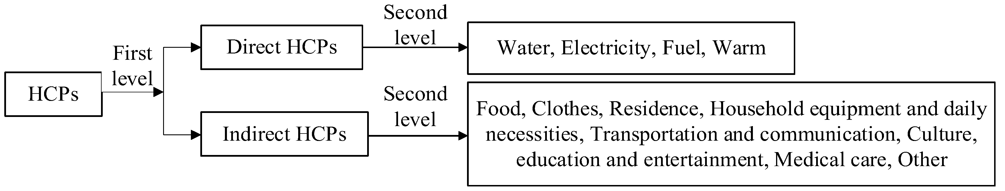
HCPs were expressed as the proportion of direct and indirect HCEX in total HCEX; the direct HCPs were divided into proportions of water, electricity, fuel and warm in direct HCEX, and the indirect HCPs were divided into proportions of eight categories in indirect HCEX. Considering the difference in income, different HCPs might account for different amounts of HCEX when the proportion is the same. If the proportion had been used for calculation, the error would be aggravated, giving it little meaning in reality. Therefore, in this paper, HCPs were defined as the amount of HCEX [45], as shown in Figure 1.

(2) Definition of green transformation HCPs

In this paper, the green transformation of HCPs is defined as HCEs no longer increasing with the growth of HCEX. The ideal scenario of green transformation is a reduction in HCEs despite an increase in HCEX. Therefore, the green transformation of HCPs could be evaluated by the decoupling relationship between HCEX and HCEs.

2.2. Methods for Calculating HCEs

HCEs include direct and indirect HCEs. Direct HCEs refer to CO₂ produced by direct use of energy, such as coal, coke, gasoline, kerosene, diesel, and natural gas consumed by heating, cooling, lighting, cooking, and other projects. Indirect HCEs refer to CO₂ generated by energy consumption in the materials production and other aspects of the products and services consumed by residents, including food, clothes, accommodation, daily necessities, transportation and communication, education, culture and entertainment, medical care, and other categories.

For calculating HCEs, this study adopted dynamic standard coal carbon emission factors (EF) [46] instead of a fixed value to convert the measurement units of EF of indirect consumption in the eight categories and EF of direct consumption of water into tCO₂/CNY. Additionally, EF of dynamic electricity and heat [47,48] were utilized to calculate HCEs of electricity and heating.

The carbon emission coefficient method and input–output consumer lifestyle approach were adopted in this study to calculate the direct and indirect HCEs from 2012 to 2018. The specific calculation steps are explained in Appendix C.

2.3. Model Construction

(1) Model of green transformation of HCPs

The Tapio decoupling method was used to measure the green transformation of direct and indirect HCPs through the following formula. The meaning of the decoupling state is shown in Appendix A:

$$e(C_x^d,D_x^d)=\left(\mathsf{\Delta }{C}_x^d/C_x^d\right)/\left(\mathsf{\Delta }{D}_x^d/D_x^d\right)$$

(1)

$$e(C_x^m,D_x^m)=\left(\mathsf{\Delta }{C}_x^m/C_x^m\right)/\left(\mathsf{\Delta }{D}_x^m/D_x^m\right)$$

(2)

In Equations (1) and (2), x (x = 1, 2, …, 10) represents the eastern, central, western, and northeastern regions, four income levels, urban and rural areas. $e(C_x^d,D_x^d)$ and $e(C_x^m,D_x^m)$ denote the decoupling indices of direct and indirect HCEX and HCEs. C^d and C^m represent direct and indirect HCEs. D^d and D^m represent direct and indirect HCEX. ΔC^d and ΔC^m are the changes in direct and indirect HCEs. ΔD^d and ΔD^m are the changes in direct and indirect HCEX. ΔC^d/C^d and ΔC^m/C^m are the changing rates of direct and indirect HCEs. ΔD^d/D^d and ΔD^m/D^m are the changing rates of direct and indirect HCEX.

(2) Decomposition model of driving factors of green transformation of HCPs

The LMDI decomposition method was used to decompose the driving factors of green transformation of direct and indirect HCPs, as shown in the following formula:

• Decomposition model of driving factors of green transformation of direct HCPs:

  $$\begin{gathered} C_x^{dt}=\sum \frac{C_{xi}^{dt}}{D_{xi}^{dt}}\times \frac{D_{xi}^{dt}}{D_x^{dt}}\times \frac{D_x^{dt}}{A_x^t}\times \frac{A_x^t}{P_x^t}\times \frac{P_x^t}{H_x^t}\times H_x^t \\ =\sum I_{xi}^{dt}\times S_{xi}^{dt}\times A{E}_x^{dt}\times A{P}_x^t\times H{S}_x^t\times H_x^t \end{gathered}$$

  (3)

In Equation (3), t represents the year, i represents four categories of direct consumption, C^d represents direct HCEs, D^d represents direct HCEX, A represents household residential area, and P represents total population. I^d represents direct household carbon intensity effect, S^d represents direct household consumption structure effect, AE represents direct household per unit residential consumption effect, AP represents household per capita residential area effect, HS represents household size effect, H represents household number effect.

The factor decomposition of the change in direct HCEs from year 0 to year t and the effect of each factor is shown as follows:

$$\Delta C_x^{dt}=C_x^{dt}-C_x^{d0}=\Delta C_{x,I}^d+\Delta C_{x,S}^d+\Delta C_{x,AE}^d+\Delta C_{x,AP}^d+\Delta C_{x,HS}^d+\Delta C_{x,H}^d$$

(4)

Direct household carbon intensity effect:

$$\Delta C_{x,I}^d=\sum \frac{C_{xi}^{dt}-C_{xi}^{d0}}{\ln C_{xi}^{dt}-\ln C_{xi}^{d0}}\times \ln \frac{I_{xi}^{dt}}{I_{xi}^{d0}}$$

Direct household consumption structure effect:

$$\Delta C_{x,S}^d=\sum \frac{C_{xi}^{dt}-C_{xi}^{d0}}{\ln C_{xi}^{dt}-\ln C_{xi}^{d0}}\times \ln \frac{S_{xi}^{dt}}{S_{xi}^{d0}}$$

Direct per square meter household residential consumption effect:

$$\Delta C_{x,AE}^d=\sum \frac{C_{xi}^{dt}-C_{xi}^{d0}}{\ln C_{xi}^{dt}-\ln C_{xi}^{d0}}\times \ln \frac{A{E}_x^{dt}}{A{E}_x^{d0}}$$

Household per capita residential area effect:

$$\Delta C_{x,AP}^d=\sum \frac{C_{xi}^{dt}-C_{xi}^{d0}}{\ln C_{xi}^{dt}-\ln C_{xi}^{d0}}\times \ln \frac{A{P}_x^t}{A{P}_x^0}$$

Household size effect:

$$\Delta C_{x,HS}^d=\sum \frac{C_{xi}^{dt}-C_{xi}^{d0}}{\ln C_{xi}^{dt}-\ln C_{xi}^{d0}}\times \ln \frac{H{S}_x^t}{H{S}_x^0}$$

Household number effect:

$$\Delta C_{x,H}^d=\sum \frac{C_{xi}^{dt}-C_{xi}^{d0}}{\ln C_{xi}^{dt}-\ln C_{xi}^{d0}}\times \ln \frac{H_x^t}{H_x^0}$$

• Decomposition model of driving factors of green transformation of indirect HCPs:

  $$\begin{gathered} C_x^{mt}\sum \frac{C_{xj}^{mt}}{D_{xj}^{mt}}\times \frac{D_{xj}^{mt}}{D_x^{mt}}\times \frac{D_x^{mt}}{R_x^t}\times \frac{R_x^t}{P_x^t}\times \frac{P_x^t}{H_x^t}\times H_x^t \\ =\sum I_{xj}^{mt}\times S_{xj}^{mt}\times C{R}_x^{mt}\times AP{C}_x^t\times H{S}_x^t\times H_x^t \end{gathered}$$

  (5)

In Equation (5), j represents eight categories of indirect consumption, C^m represents indirect HCEs, D^m represents indirect HCEX, and R represents household net income. I^m represents the indirect household carbon intensity effect, S^m represents the indirect household consumption structure effect, CR represents the household consumption propensity effect, and APC represents the household per capita net income effect.

The factor decomposition of the change in indirect HCEs from year 0 to year t and the effect of each factor is shown as follows:

$$\Delta C_x^{mt}=C_x^{mt}-C_x^{m0}=\Delta C_{x,I}^m+\Delta C_{x,S}^m+\Delta C_{x,CR}^m+\Delta C_{x,APC}^m+\Delta C_{x,HS}^m+\Delta C_{x,H}^m$$

(6)

Indirect household carbon intensity effect:

$$\Delta C_{x,I}^m=\sum \frac{C_{xj}^{mt}-C_{xj}^{m0}}{\ln C_{xj}^{mt}-\ln C_{xj}^{m0}}\times \ln \frac{I_{xj}^{mt}}{I_{xj}^{m0}}$$

Indirect household consumption structure effect:

$$\Delta C_{x,S}^m=\sum \frac{C_{xj}^{mt}-C_{xj}^{m0}}{\ln C_{xj}^{mt}-\ln C_{xj}^{m0}}\times \ln \frac{S_{xj}^{mt}}{S_{xj}^{m0}}$$

Household consumption propensity effect:

$$\Delta C_{x,CR}^m=\sum \frac{C_{xj}^{mt}-C_{xj}^{m0}}{\ln C_{xj}^{mt}-\ln C_{xj}^{m0}}\times \ln \frac{C{R}_x^{mt}}{C{R}_x^{m0}}$$

Household per capita net income effect:

$$\Delta C_{x,APC}^m=\sum \frac{C_{xj}^{mt}-C_{xj}^{m0}}{\ln C_{xj}^{mt}-\ln C_{xj}^{m0}}\times \ln \frac{AP{C}_x^t}{AP{C}_x^0}$$

Household size effect:

$$\Delta C_{x,HS}^m=\sum \frac{C_{xj}^{mt}-C_{xj}^{m0}}{\ln C_{xj}^{mt}-\ln C_{xj}^{m0}}\times \ln \frac{H{S}_x^t}{H{S}_x^0}$$

Household number effect:

$$\Delta C_{x,H}^m=\sum \frac{C_{xj}^{mt}-C_{xj}^{m0}}{\ln C_{xj}^{mt}-\ln C_{xj}^{m0}}\times \ln \frac{H_x^t}{H_x^0}$$

Extended factor decomposition models of green transformation of direct and indirect HCPs are shown in the following formulas:

$$\begin{gathered} e(C_x^d,D_x^d)=\frac{\mathsf{\Delta }{C}_x^{dt}/C_x^{d0}}{\mathsf{\Delta }{D}_x^{dt}/D_x^{d0}} \\ =\frac{\mathsf{\Delta }{C}_{xI}^{dt}/C_x^{d0}}{\mathsf{\Delta }{D}_x^{dt}/D_x^{d0}}+\frac{\mathsf{\Delta }{C}_{xS}^{dt}/C_x^{d0}}{\mathsf{\Delta }{D}_x^{dt}/D_x^{d0}}+\frac{\mathsf{\Delta }{C}_{xAE}^{dt}/C_x^{d0}}{\mathsf{\Delta }{D}_x^{dt}/D_x^{d0}}+\frac{\mathsf{\Delta }{C}_{xAP}^{dt}/C_x^{d0}}{\mathsf{\Delta }{D}_x^{dt}/D_x^{d0}}+\frac{\mathsf{\Delta }{C}_{xHS}^{dt}/C_x^{d0}}{\mathsf{\Delta }{D}_x^{dt}/D_x^{d0}}+\frac{\mathsf{\Delta }{C}_{xH}^{dt}/C_x^{d0}}{\mathsf{\Delta }{D}_x^{dt}/D_x^{d0}} \\ =e_{x,I}^d+e_{x,S}^d+e_{x,AE}^d+e_{x,AP}^d+e_{x,HS}^d+e_{x,H}^d \end{gathered}$$

(7)

In Equation (7), $e_{x,I}^d, e_{x,S}^d, e_{x,AE}^d, e_{x,AP}^d, e_{x,HS}^d, e_{x,H}^d$ are respectively the decoupling indexes of direct household carbon intensity, direct household consumption structure, direct household per square meter residential consumption, household per capita residential area, household size, and household number.

$$\begin{gathered} e(C_x^m,D_x^m)=\frac{\mathsf{\Delta }{C}_x^{mt}/C_x^{m0}}{\mathsf{\Delta }{D}_x^{mt}/D_x^{m0}} \\ =\frac{\mathsf{\Delta }{C}_{xI}^{mt}/C_x^{m0}}{\mathsf{\Delta }{D}_x^{mt}/D_x^{m0}}+\frac{\mathsf{\Delta }{C}_{xS}^{mt}/C_x^{m0}}{\mathsf{\Delta }{D}_x^{mt}/D_x^{m0}}+\frac{\mathsf{\Delta }{C}_{xCR}^{mt}/C_x^{m0}}{\mathsf{\Delta }{D}_x^{mt}/D_x^{m0}}+\frac{\mathsf{\Delta }{C}_{xAPC}^{mt}/C_x^{m0}}{\mathsf{\Delta }{D}_x^{mt}/D_x^{m0}}+\frac{\mathsf{\Delta }{C}_{xHS}^{mt}/C_x^{m0}}{\mathsf{\Delta }{D}_x^{mt}/D_x^{m0}}+\frac{\mathsf{\Delta }{C}_{xH}^{mt}/C_x^{m0}}{\mathsf{\Delta }{D}_x^{mt}/D_x^{m0}} \\ =e_{x,I}^m+e_{x,S}^m+e_{x,CR}^m+e_{x,APC}^m+e_{x,HS}^m+e_{x,H}^m \end{gathered}$$

(8)

In Equation (8), $e_{x,I}^m, e_{x,S}^m, e_{x,CR}^m, e_{x,APC}^m, e_{x,HS}^m, e_{x,H }^m$ are respectively the decoupling indexes of indirect household carbon intensity, indirect household consumption structure, household consumption propensity, household per capita net income, household size, and household number.

(3) Marginal effect analysis

Based on the results of driving factors of green transformation of HCPs, it can be seen that among the driving factors of direct HCPs, per capita residential area and household size exhibited a significant negative impact. Among the driving factors of indirect HCPs, household income [49] and household size [50] exhibited significant positive and negative impacts on HCEs. Thus, this paper analyzes the marginal effects of residential area, household income, and household size on HCEs. The formula is as follows:

$$M{C}_i=\frac{\Delta C}{\Delta i}=\frac{d\left(C_2-C_1\right)}{d\left(i_2-i_1\right)}=d\left(C_2-C_1\right)=d{C}_2-d{C}_1=C_2-C_1$$

(9)

i = (I, S, A), where I, S, and A represent household income, household size, and residential area, respectively. C represents HCEs.

This paper introduces the growth rate of HCEs to reflect the relative change of the marginal effect of residential area, household income, and household size on HCEs. The formula is as follows:

$$M{R}_i=\frac{\Delta C}{C_1}=\frac{C_2-C_1}{C_1}=\frac{M{C}_i}{C_1}$$

(10)

2.4. Data Sources

Data of HCEX and driving factors were derived from the China Family Panel Studies (CFPS) database in 2012–2018. Data for calculating CF of direct and indirect consumption, CF of dynamic electricity, heating, and standard coal were derived from the China Statistical Yearbook and China Energy Statistical Yearbook. Data of average low calorific value are from the general principles for the calculation of comprehensive consumption, and the carbon content per unit calorific value and oxidation rate were from the Provincial Inventory of Greenhouse Gas Emissions Guide. When calculating direct energy consumption based on HCEX, prices of coal, gasoline, diesel, liquefied petroleum gas, natural gas, water, and electricity were derived from the Wind database, and prices of warm were derived from the China Urban Heating Association. The reason for using data from 2012 to 2018 in this study is that the energy consumption is calculated by dividing the consumption amount in the CFPS database by the prices of each energy source. However, the prices of different energy sources were updated only to 2018.

3. Results and Discussions

3.1. Analysis of HCEs and HCPs

This study analyzed the direct and indirect HCEs and HCPs from three perspectives: regions, income levels, and urban–rural areas. According to the classification of the China Statistical Yearbook, China includes the eastern, central, western, and northeastern regions. Simultaneously, according to household per capita net income in CFPS, households were divided into four income levels, with 0~25% representing low-income households; 25~50% representing low-middle-income households; 50~75% representing high-middle-income households; and 75~100% representing high-income households.

(1) Descriptive statistical analysis of HCPs and HCEs

Characteristics of HCPs and HCEs were analyzed in view of total level, and direct–indirect level.

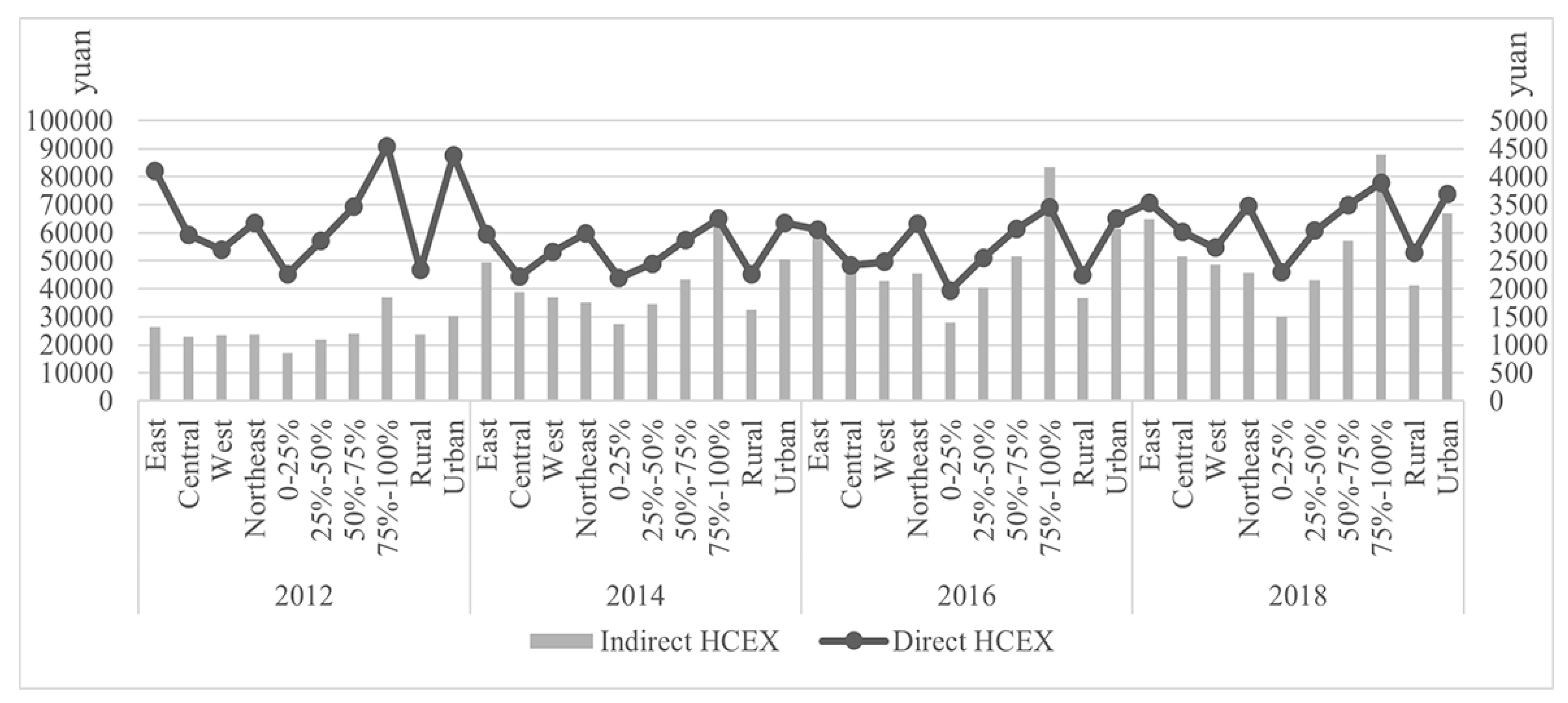
In terms of total HCPs and HCEs, as depicted in Figure 2, the proportion of indirect HCEX in China during the period 2012–2018 was considerably higher compared with that of direct HCEX. From the regional perspective, the indirect HCEX in the eastern region and the direct HCEX in both eastern and northeastern regions were higher each year than those in other regions. From the income perspective, there was an increasing trend observed each year for both direct and indirect HCEX as income levels increased. From the urban–rural perspective, the direct and indirect HCEX in urban areas surpassed those in rural areas, and both increased annually.

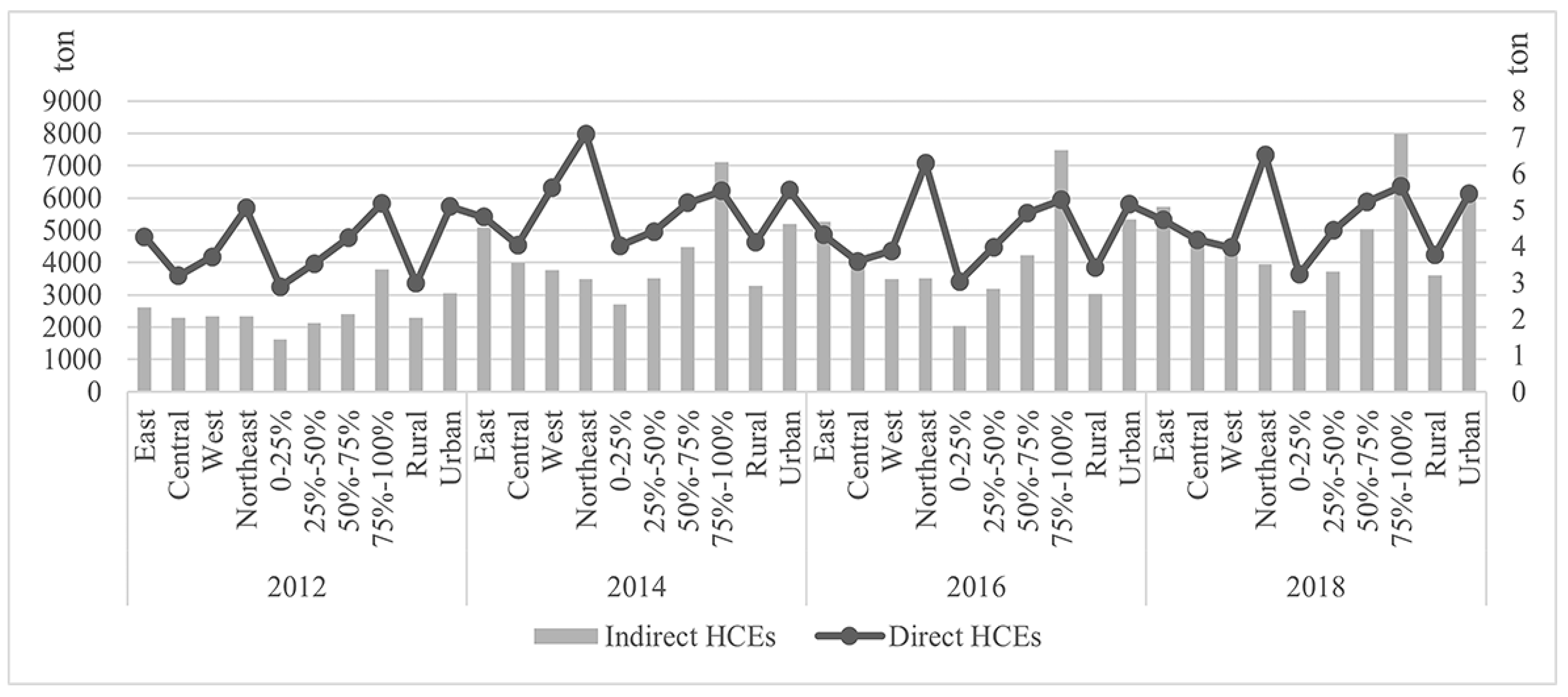
As shown in Figure 3, there was a notable alignment between the trends in indirect HCEs and indirect HCPs in 2012–2018. Similarly, the trends in direct HCEs were consistent with direct HCPs across income levels and urban–rural areas. From the regional perspective, direct HCEs were highest in northeast China and lowest in central China.

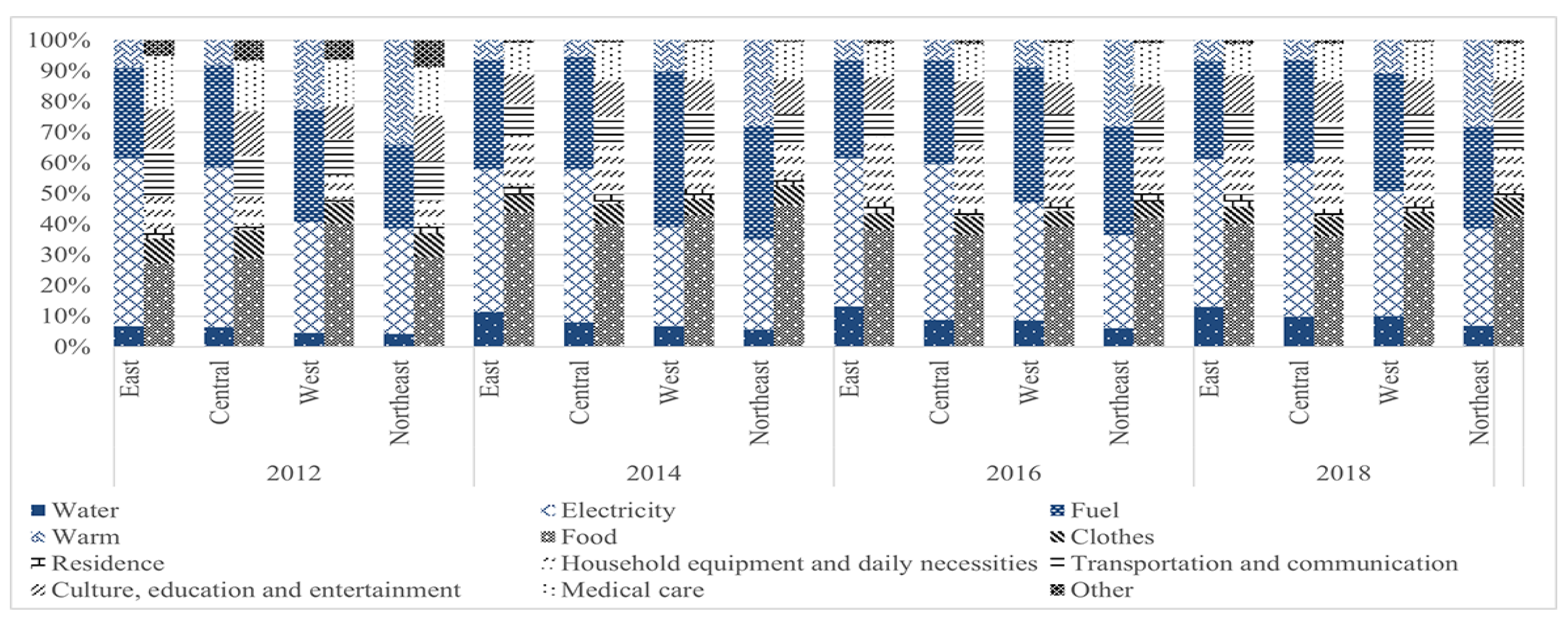
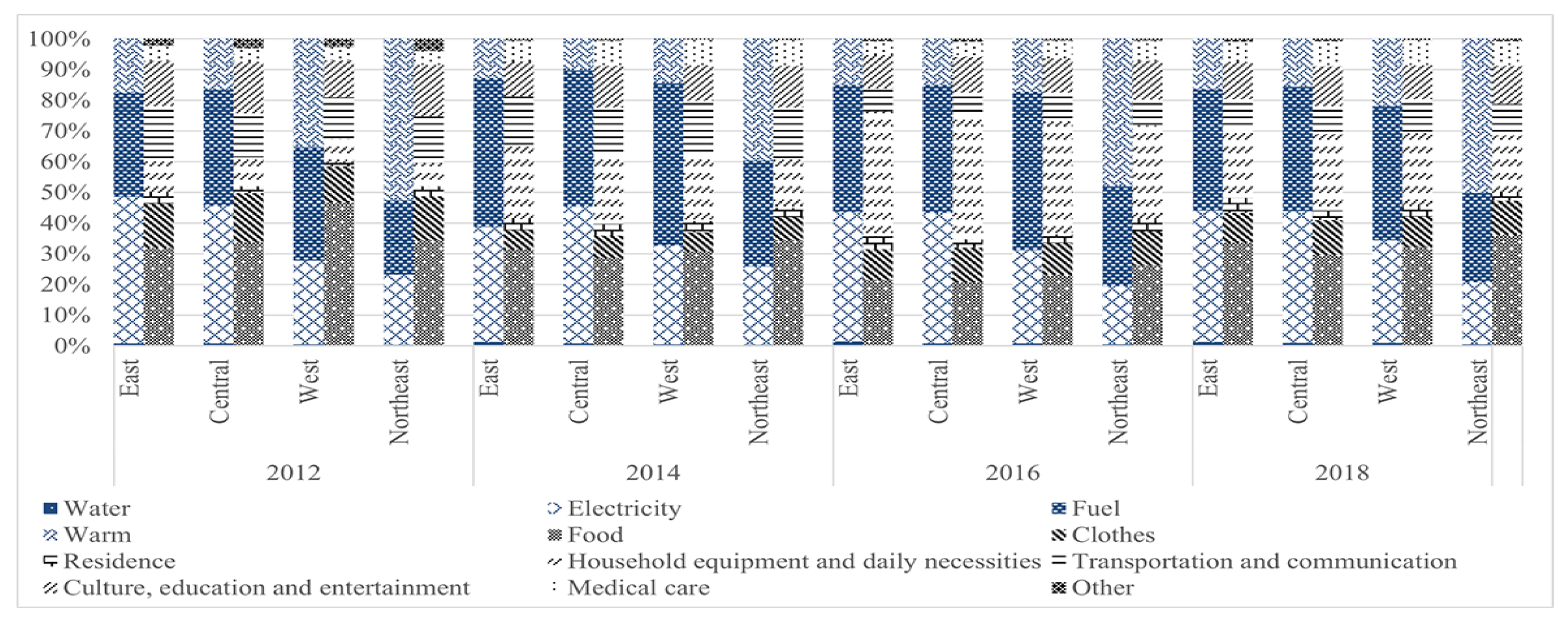
In terms of direct and indirect HCPs and HCEs, from the regional perspective, Figure 4 illustrates that the proportion of electricity and fuel consumption expenditure (CEX) of the direct HCPs in China was the highest from 2012 to 2018, and warm CEX in northeast China occupied a relatively high proportion.

Food, household equipment and daily necessities occupied the highest proportion of indirect HCPs in China from 2012 to 2018. The proportion of food CEX in each region presented a trend from increasing to decreasing in 2012–2016, and remained almost unchanged from 2016 to 2018. However, the proportion of CEX assigned to household equipment and daily necessities increased annually from 2012 to 2016 but decreased from 2016 to 2018, in all regions.

Figure 5 illustrates that fuel and electricity contributed the most to direct HCEs. The proportion of CEs from fuel presented a decreasing trend annually. However, northeast China exhibited lower CEs from fuel and electricity but higher CEs from warm.

The proportion of CEs from food decreased annually from 2012 to 2016 and increased slightly from 2016 to 2018. The proportion of CEs from household equipment and daily necessities in all regions increased annually from 2012 to 2016 but decreased from 2016 to 2018.

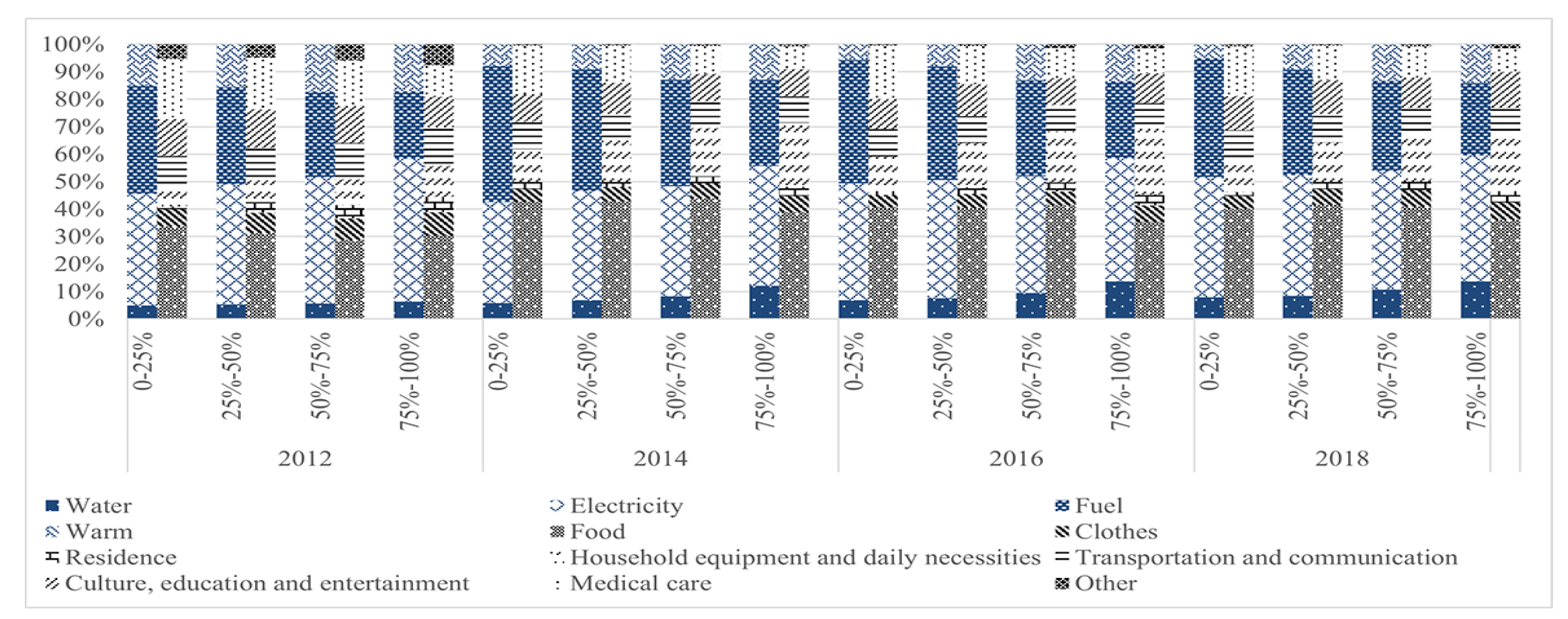
From the income perspective, Figure 6 indicates that the highest proportion of HCPs in China was allocated to electricity and fuel from 2012 to 2018. As income levels increased, the proportion of fuel CEX decreased, whereas the proportion of electricity CEX increased.

The highest proportions of indirect HCPs in China from 2012 to 2018 were for food, household equipment and daily necessities. The proportion of food CEX of all income groups presented a trend of increasing to decreasing from 2012 to 2016 and remained relatively stable from 2016 to 2018. However, the proportions of CEX for household equipment and daily necessities increased annually from 2012 to 2016 but decreased from 2016 to 2018. Additionally, as income level increased, the proportion of food CEX decreased while those of household equipment and daily necessities increased.

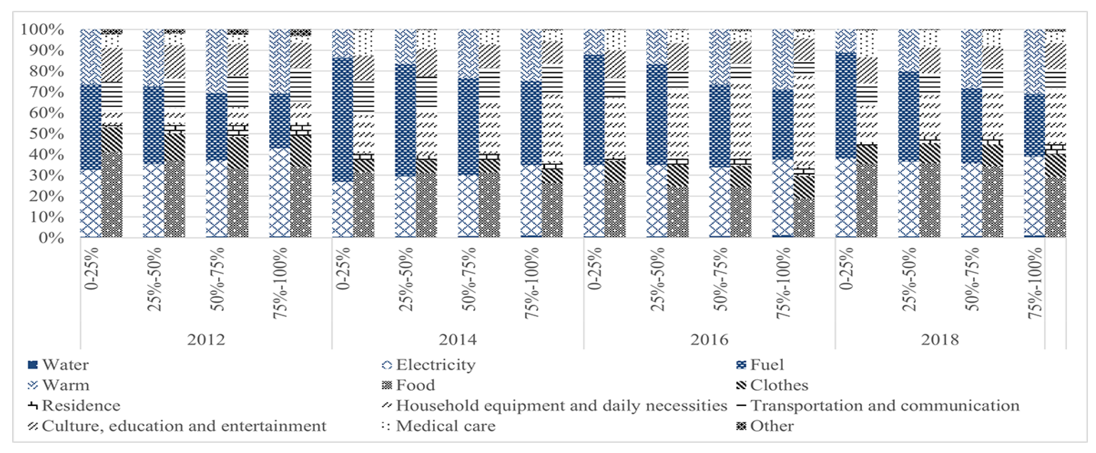
Figure 7 indicates that the highest proportion of HCEs from direct consumption by residents was attributed to fuel and electricity, and the proportion of CEs from fuel decreased annually as income level increased.

The proportion of CEs from food consumption of all income groups decreased annually from 2012 to 2016 but increased from 2016 to 2018. Conversely, the proportion of CEs stemming from household equipment and daily necessities exhibited an increasing trend from 2012 to 2016 but experienced a decline from 2016 to 2018.

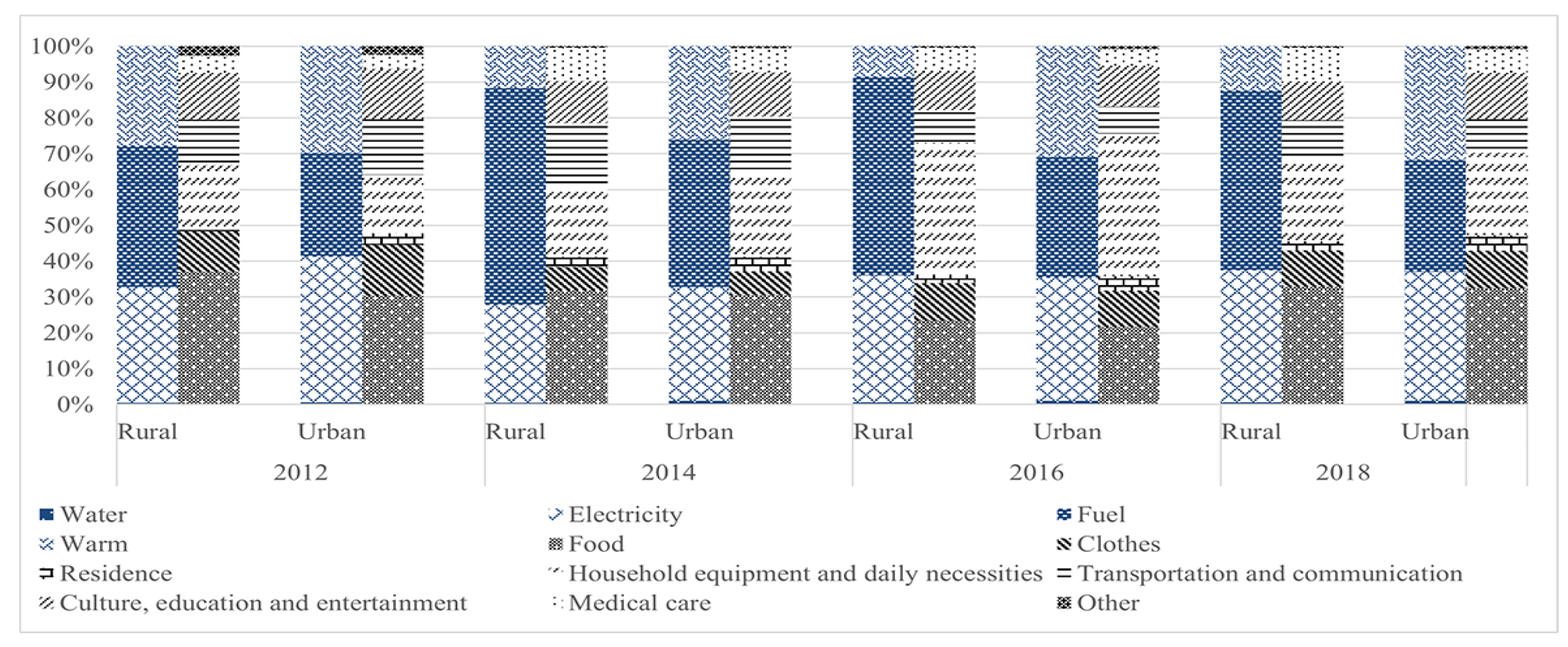
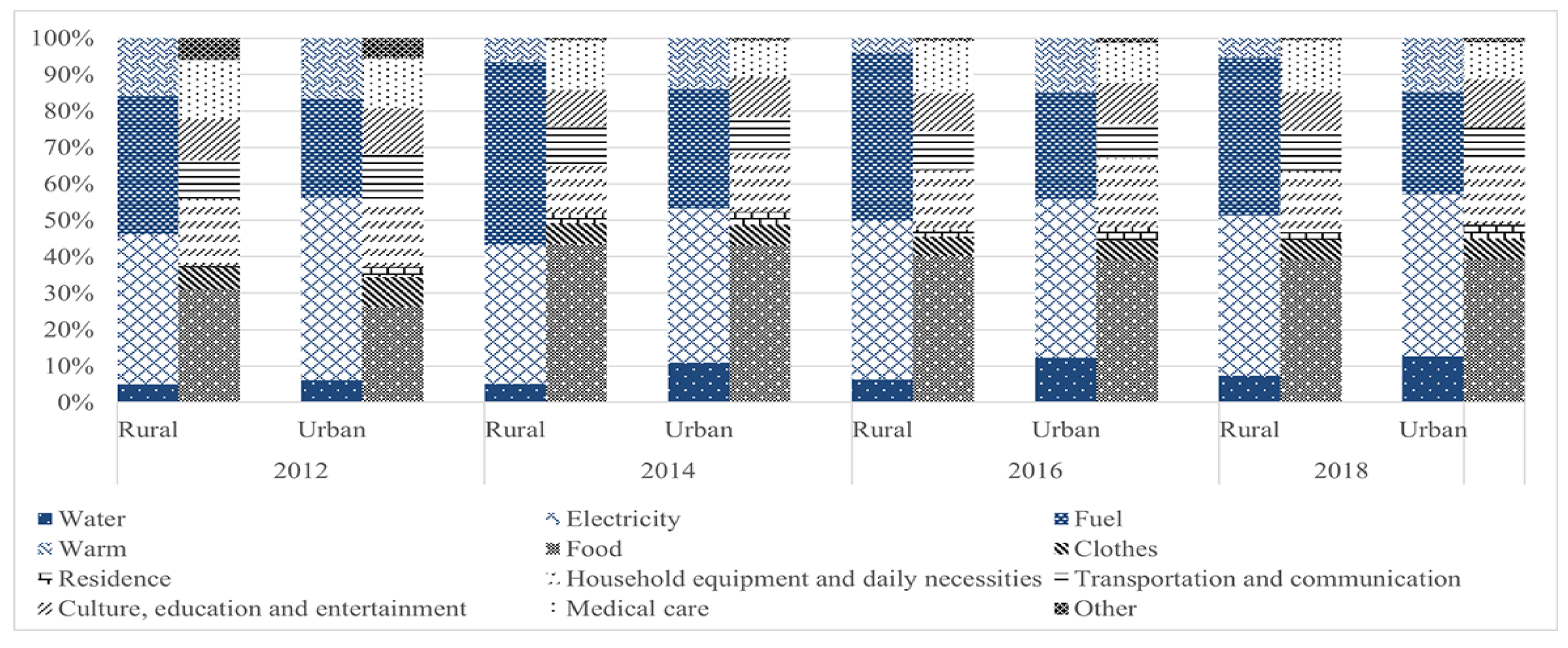
From the urban–rural perspective, Figure 8 indicates that the proportions of electricity and fuel CEX were highest in both urban and rural areas. Notably, the proportion of fuel CEX was higher in rural areas than in urban areas from 2012 to 2018.

Food, household equipment, and daily necessities constituted the majority of indirect HCPs in China from 2012 to 2018. Specifically, the proportion of food CEX increased from 2012 to 2014 but decreased from 2014 to 2018. However, the proportions of CEX for household equipment and daily necessities declined from 2012 to 2014 but increased from 2014 to 2018.

Figure 9 indicated that the highest proportion of direct HCEs was attributed to fuel and warm. Notably, the proportion of CEs from fuel declined annually, and it was higher in rural areas than in urban areas, but the proportion of CEs from warm was lower in rural areas than in urban areas.

The proportion of CEs from food decreased annually from 2012 to 2016 but increased from 2016 to 2018. Conversely, the proportions of CEs from household equipment and daily necessities increased from 2012 to 2016 but declined from 2016 to 2018.

(2) Analysis of dominant types of HCPs

This paper classifies HCPs through various types of HCEX and analyzes the dominant types of HCPs across regions, income levels, and urban–rural areas, based on the traditional definition of HCPs. Food, household equipment and daily necessities are classified as necessities. The dominant types of direct and indirect HCPs are shown in

Table 1. Dominant types of direct HCPs.

Research Perspectives		Dominant Types of Direct HCPs
		2012	2014	2016	2018
Regions	East	Electricity	Electricity	Electricity	Electricity
	Central	Electricity	Electricity	Electricity	Electricity
	West	Fuel	Fuel	Fuel	Electricity
	Northeast	Electricity	Fuel	Fuel	Fuel
Income levels	Low income	Electricity	Fuel	Fuel	Electricity
	Low-middle income	Electricity	Fuel	Electricity	Electricity
	High-middle income	Electricity	Electricity	Electricity	Electricity
	High income	Electricity	Electricity	Electricity	Electricity
Urban–rural	Rural	Electricity	Fuel	Fuel	Electricity
	Urban	Electricity	Electricity	Electricity	Electricity

and

Table 2. Dominant types of indirect HCPs.

Research Perspectives		Dominant Types of Indirect HCPs
		2012	2014	2016	2018
Regions	East	Necessities + Health + Transportation	Necessities + Health	Necessities + Health	Necessities + Education
	Central	Necessities + Health + Education	Necessities + Health	Necessities + Health	Necessities + Education
	West	Necessities + Health + Transportation	Necessities + Health	Necessities + Health	Necessities + Health
	Northeast	Necessities + Health + Education	Necessities + Health + Education	Necessities + Health	Necessities + Education
Income levels	Low income	Necessities + Health + Education	Necessities + Health	Necessities + Health	Necessities + Health
	Low-middle income	Necessities + Health +Education	Necessities + Health	Necessities + Health	Necessities + Health
	High-middle income	Necessities + Health + Education	Necessities + Health	Necessities + Health	Necessities + Health
	High income	Necessities + Health + Transportation	Necessities + Education	Necessities + Education	Necessities + Education
Urban–rural	Rural	Necessities + Health	Necessities + Health	Necessities + Health	Necessities + Health
	Urban	Necessities + Health	Necessities + Education	Necessities + Education	Necessities + Education

.

Obviously, in 2012–2018, the dominant type of direct HCPs was mainly electricity, while fuel mainly appeared in less developed areas like western and northeastern regions, low-income groups, and rural areas. Dominant types of indirect HCPs were mainly necessities and health, while transportation and education mainly appeared in eastern and central regions, high-income groups, and urban areas.

3.2. Measurement of Green Transformation of HCPs

The green transformation of HCPs was measured from three perspectives: regions, income levels, and urban–rural areas.

(1) Measurement of green transformation of direct HCPs

According to Equation (1), measurement of green transformation of direct HCPs was conducted in view of direct HCPs, including four categories of direct HCPs. The results are shown in

Table A2. Green transformation measurement of direct HCPs from 2012 to 2018.

Research Perspectives		Year	Total	Water	Electricity	Fuel	Warm
Regions	East	2012–2014	Strong Negative Decoupling	Strong Negative Decoupling	Strong Negative Decoupling	Strong Negative Decoupling	Weak Negative Decoupling
		2014–2016	Strong Decoupling	Weak Decoupling	Strong Decoupling	Strong Decoupling	Weak Decoupling
		2016–2018	Weak Decoupling	Weak Decoupling	Weak Decoupling	Weak Decoupling	Weak Decoupling
	Central	2012–2014	Strong Negative Decoupling	Strong Negative Decoupling	Strong Negative Decoupling	Strong Negative Decoupling	Weak Negative Decoupling
		2014–2016	Strong Decoupling	Weak Decoupling	Strong Decoupling	Strong Decoupling	Weak Decoupling
		2016–2018	Weak Decoupling	Weak Decoupling	Weak Decoupling	Weak Decoupling	Weak Decoupling
	West	2012–2014	Strong Negative Decoupling	Strong Negative Decoupling	Strong Negative Decoupling	Strong Negative Decoupling	Recessionary Decoupling
		2014–2016	Recessionary Decoupling	Strong Negative Decoupling	Weak Negative Decoupling	Recessionary Linkage	Weak Negative Decoupling
		2016–2018	Weak Decoupling	Weak Decoupling	Weak Decoupling	Strong Decoupling	Weak Decoupling
	Northeast	2012–2014	Strong Negative Decoupling	Strong Negative Decoupling	Strong Negative Decoupling	Strong Negative Decoupling	Strong Negative Decoupling
		2014–2016	Strong Decoupling	Weak Decoupling	Strong Decoupling	Strong Decoupling	Weak Decoupling
		2016–2018	Weak Decoupling	Weak Decoupling	Weak Decoupling	Strong Decoupling	Weak Decoupling
Income levels	0–25%	2012–2014	Strong Negative Decoupling	Strong Negative Decoupling	Strong Negative Decoupling	Strong Negative Decoupling	Weak Negative Decoupling
		2014–2016	Recessionary Decoupling	Strong Negative Decoupling	Strong Negative Decoupling	Recessionary Decoupling	Weak Negative Decoupling
		2016–2018	Weak Decoupling	Weak Decoupling	Weak Decoupling	Strong Decoupling	Strong Decoupling
	25–50%	2012–2014	Strong Negative Decoupling	Strong Negative Decoupling	Strong Negative Decoupling	Strong Negative Decoupling	Weak Negative Decoupling
		2014–2016	Strong Decoupling	Weak Decoupling	Weak Decoupling	Strong Decoupling	Strong Decoupling
		2016–2018	Weak Decoupling	Weak Decoupling	Weak Decoupling	Strong Decoupling	Weak Decoupling
	50–75%	2012–2014	Strong Negative Decoupling	Strong Negative Decoupling	Strong Negative Decoupling	Strong Negative Decoupling	Strong Negative Decoupling
		2014–2016	Strong Decoupling	Weak Decoupling	Weak Decoupling	Strong Decoupling	Weak Decoupling
		2016–2018	Weak Decoupling	Weak Decoupling	Weak Decoupling	Strong Decoupling	Weak Decoupling
	75–100%	2012–2014	Strong Negative Decoupling	Strong Negative Decoupling	Strong Negative Decoupling	Strong Negative Decoupling	Strong Negative Decoupling
		2014–2016	Strong Decoupling	Weak Decoupling	Weak Decoupling	Strong Decoupling	Weak Decoupling
		2016–2018	Weak Decoupling	Weak Decoupling	Weak Decoupling	Strong Decoupling	Weak Decoupling
Urban–rural	Rural	2012–2014	Strong Negative Decoupling	Strong Negative Decoupling	Strong Negative Decoupling	Strong Negative Decoupling	Recessionary Linkage
		2014–2016	Recessionary Decoupling	Strong Negative Decoupling	Weak Negative Decoupling	Recessionary Decoupling	Recessionary Linkage
		2016–2018	Weak Decoupling	Weak Decoupling	Weak Decoupling	Strong Decoupling	Weak Decoupling
	Urban	2012–2014	Strong Negative Decoupling	Strong Negative Decoupling	Strong Negative Decoupling	Strong Negative Decoupling	Strong Negative Decoupling
		2014–2016	Strong Decoupling	Weak Decoupling	Strong Decoupling	Strong Decoupling	Weak Decoupling
		2016–2018	Weak Decoupling	Weak Decoupling	Weak Decoupling	Strong Decoupling	Weak Decoupling

of Appendix B.

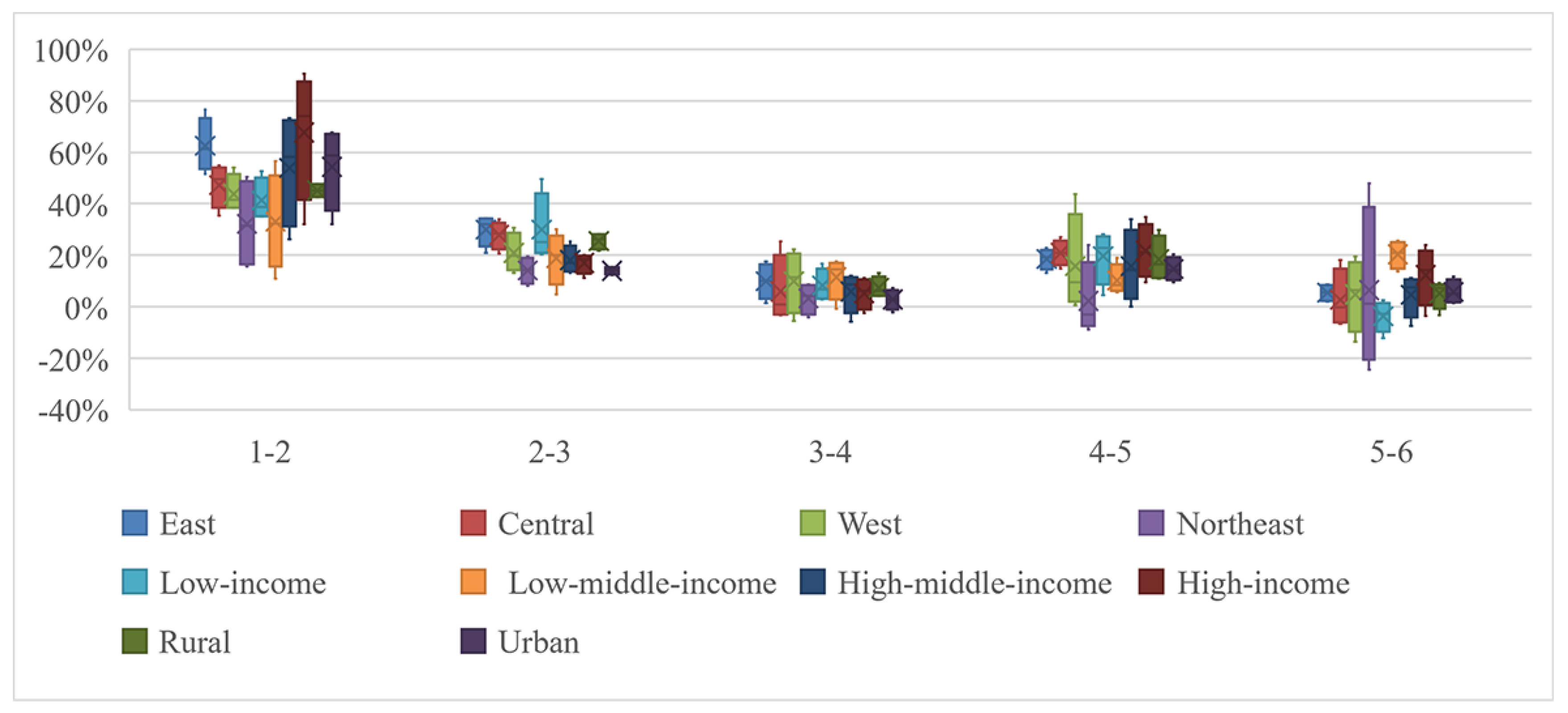
In terms of green transformation of direct HCPs, from the time perspective, all the regions, income levels, and urban–rural areas (all perspectives) witnessed strong negative decoupling from 2012 to 2014, which indicated that direct HCEX decreased while HCEs increased, portraying the worst stage of green transformation of direct HCPs. This could be attributed to the global financial crisis, which weakened the global economy and had a long-term impact on economic development in China.

Recessionary decoupling was observed in the western region, low-income groups, and rural areas from 2014 to 2016, which signified a decrease in both direct HCEX and HCEs, with HCEs reducing faster than HCEX. The strong decoupling observed from the other perspectives represented the most desirable state of green transformation. This could be attributed to the low-carbon pilot initiatives launched by the National Development and Reform Commission, which took place in six provinces and 36 cities, with two batches implemented in 2010 and 2012.

All perspectives witnessed weak decoupling from 2016 to 2018, indicating a more ideal state of green transformation. This included a focus on resolving problems of overcapacity in the coal industry nationwide in 2016, combined with the implementation of the National Water Saving Action Plan issued by the National Development and Reform Commission, that together resulted in a significant reduction in HCEs.

From the regional perspective, during the periods 2012–2014, 2014–2016, and 2016–2018, the decoupling in east, central, and northeast China transitioned from strong negative decoupling to strong decoupling to weak decoupling. Similarly, the western region transformed from strong negative decoupling to recessionary decoupling to weak decoupling. The positive trend in the green transformation could be attributed to clean alternative strategies like replacing coal with gas and electricity, proposed in the 13th Five-Year Plan for Energy Development, which led to a slower increase in direct HCEs compared with HCEX.

From the income perspective, the low-income class transitioned from strong negative decoupling to recessionary decoupling to weak decoupling, while other income groups transformed from strong negative decoupling to strong decoupling to weak decoupling. This positive trend could be attributed to the 13th Five-Year Plan for the Development of Renewable Energy in 2016, which emphasized the development of hydropower, wind power, solar energy, and biomass energy, thereby reducing HCEs.

From the urban–rural perspective, rural areas transitioned from strong negative decoupling to recessionary decoupling to weak decoupling, while urban areas transitioned from strong negative decoupling to strong decoupling to weak decoupling. This positive trend could be attributed to the 13th Five-Year Plan for National Rural Economic Development issued in 2016, which emphasized the joint promotion of agricultural modernization, informatization, greenization, urbanization, the construction of beautiful countryside, and the coordinated development of urban–rural areas.

In terms of the green transformation of four categories of direct HCPs, water displayed strong negative decoupling from 2012 to 2014, indicating the poorest state of green transformation. However, it presented weak decoupling from 2014 to 2018, signifying a more favorable state of green transformation. Conversely, electricity demonstrated strong decoupling from 2012 to 2014 and weak decoupling from 2016 to 2018. However, it fluctuated between strong and weak decoupling from 2014 to 2016, with only the western regions, rural areas, and low-income groups showing weak and strong negative decoupling. Fuel exhibited strong decoupling from 2012 to 2014. However, it transitioned between strong and weak decoupling from 2014 to 2018, with certain perspectives experiencing recessionary decoupling and recessionary linkage. Warm mainly displayed weak negative decoupling from 2012 to 2014. However, it primarily exhibited weak decoupling from 2014 to 2018, with certain perspectives showing strong decoupling, weak negative decoupling, recessionary linkage, and recessionary decoupling.

(2) Measurement of green transformation of indirect HCPs

According to Equation (2), measurement of green transformation of indirect HCPs was conducted in view of indirect HCPs, including eight categories of indirect HCPs. The results are shown in

Table A3. Green transformation measurement of indirect HCPs from 2012 to 2018.

Research Perspectives		Year	Total	Food	Clothes	Residence	Household Equipment and Daily Necessities	Transportation and Communication	Culture, Education and Entertainment	Medical Care	Other
Regions	East	2012–2014	Expansionary Linkage	Weak Decoupling	Strong Decoupling	Weak Decoupling	Weak Decoupling	Weak Decoupling	Weak Decoupling	Weak Decoupling	Strong Decoupling
		2014–2016	Weak Decoupling	Strong Decoupling	Weak Decoupling	Weak Decoupling	Weak Decoupling	Strong Decoupling	Strong Decoupling	Strong Decoupling	Weak Decoupling
		2016–2018	Expansionary Negative Decoupling	Expansionary Negative Decoupling	Weak Decoupling	Weak Decoupling	Strong Decoupling	Weak Decoupling	Weak Decoupling	Weak Decoupling	Weak Decoupling
	Central	2012–2014	Expansionary Linkage	Weak Decoupling	Strong Decoupling	Weak Decoupling	Weak Decoupling	Weak Decoupling	Weak Decoupling	Weak Decoupling	Strong Decoupling
		2014–2016	Weak Decoupling	Strong Decoupling	Weak Decoupling	Strong Decoupling	Weak Decoupling	Strong Decoupling	Strong Decoupling	Strong Decoupling	Weak Decoupling
		2016–2018	Expansionary Negative Decoupling	Expansionary Negative Decoupling	Weak Decoupling	Weak Decoupling	Strong Decoupling	Weak Decoupling	Weak Decoupling	Weak Decoupling	Weak Decoupling
	West	2012–2014	Expansionary Linkage	Weak Decoupling	Strong Decoupling	Weak Decoupling	Weak Decoupling	Weak Decoupling	Weak Decoupling	Weak Decoupling	Strong Decoupling
		2014–2016	Strong Decoupling	Strong Decoupling	Weak Decoupling	Strong Decoupling	Weak Decoupling	Strong Decoupling	Strong Decoupling	Strong Decoupling	Weak Decoupling
		2016–2018	Expansionary Negative Decoupling	Expansionary Negative Decoupling	Weak Decoupling	Weak Decoupling	Strong Decoupling	Weak Decoupling	Weak Decoupling	Weak Decoupling	Strong Decoupling
	Northeast	2012–2014	Expansionary Linkage	Weak Decoupling	Strong Decoupling	Weak Decoupling	Weak Decoupling	Weak Decoupling	Weak Decoupling	Weak Decoupling	Strong Decoupling
		2014–2016	Weak Decoupling	Strong Decoupling	Weak Decoupling	Weak Decoupling	Weak Decoupling	Strong Decoupling	Strong Decoupling	Strong Decoupling	Weak Decoupling
		2016–2018	Expansionary Negative Decoupling	Expansionary Negative Decoupling	Weak Decoupling	Strong Decoupling	Strong Decoupling	Weak Decoupling	Weak Decoupling	Weak Decoupling	Weak Decoupling
Income levels	0–25%	2012–2014	Expansionary Negative Decoupling	Weak Decoupling	Strong Decoupling	Weak Decoupling	Weak Decoupling	Weak Decoupling	Weak Decoupling	Weak Decoupling	Strong Decoupling
		2014–2016	Strong Decoupling	Strong Decoupling	Weak Decoupling	Strong Decoupling	Weak Decoupling	Strong Decoupling	Strong Decoupling	Strong Decoupling	Strong Decoupling
		2016–2018	Expansionary Negative Decoupling	Expansionary Negative Decoupling	Weak Decoupling	Weak Decoupling	Strong Decoupling	Weak Decoupling	Weak Decoupling	Weak Decoupling	Weak Decoupling
	25–50%	2012–2014	Expansionary Linkage	Weak Decoupling	Strong Decoupling	Strong Decoupling	Weak Decoupling	Weak Decoupling	Weak Decoupling	Weak Decoupling	Strong Decoupling
		2014–2016	Strong Decoupling	Strong Decoupling	Weak Decoupling	Weak Decoupling	Weak Decoupling	Strong Decoupling	Strong Decoupling	Strong Decoupling	Weak Decoupling
		2016–2018	Expansionary Negative Decoupling	Expansionary Negative Decoupling	Weak Decoupling	Weak Decoupling	Strong Decoupling	Weak Decoupling	Weak Decoupling	Weak Decoupling	Weak Decoupling
	50–75%	2012–2014	Expansionary Linkage	Weak Decoupling	Strong Decoupling	Strong Decoupling	Weak Decoupling	Weak Decoupling	Weak Decoupling	Weak Decoupling	Strong Decoupling
		2014–2016	Strong Decoupling	Strong Decoupling	Weak Decoupling	Weak Decoupling	Weak Decoupling	Strong Decoupling	Strong Decoupling	Strong Decoupling	Weak Decoupling
		2016–2018	Expansionary Negative Decoupling	Expansionary Negative Decoupling	Weak Decoupling	Weak Decoupling	Strong Decoupling	Weak Decoupling	Weak Decoupling	Weak Decoupling	Strong Decoupling
	75–100%	2012–2014	Expansionary Linkage	Weak Decoupling	Strong Decoupling	Weak Decoupling	Weak Decoupling	Weak Decoupling	Weak Decoupling	Weak Decoupling	Strong Decoupling
		2014–2016	Weak Decoupling	Strong Decoupling	Weak Decoupling	Weak Decoupling	Weak Decoupling	Strong Decoupling	Strong Decoupling	Strong Decoupling	Weak Decoupling
		2016–2018	Expansionary Negative Decoupling	Expansionary Negative Decoupling	Weak Decoupling	Weak Decoupling	Strong Decoupling	Weak Decoupling	Weak Decoupling	Weak Decoupling	Weak Decoupling
Urban–rural	Rural	2012–2014	Expansionary Linkage	Weak Decoupling	Strong Decoupling	Weak Decoupling	Weak Decoupling	Weak Decoupling	Weak Decoupling	Weak Decoupling	Strong Decoupling
		2014–2016	Strong Decoupling	Strong Decoupling	Weak Decoupling	Strong Decoupling	Weak Decoupling	Strong Decoupling	Strong Decoupling	Strong Decoupling	Weak Decoupling
		2016–2018	Expansionary Negative Decoupling	Expansionary Negative Decoupling	Weak Decoupling	Weak Decoupling	Strong Decoupling	Weak Decoupling	Weak Decoupling	Weak Decoupling	Weak Decoupling
	Urban	2012–2014	Expansionary Linkage	Weak Decoupling	Strong Decoupling	Weak Decoupling	Weak Decoupling	Weak Decoupling	Weak Decoupling	Weak Decoupling	Strong Decoupling
		2014–2016	Weak Decoupling	Strong Decoupling	Weak Decoupling	Weak Decoupling	Weak Decoupling	Strong Decoupling	Strong Decoupling	Strong Decoupling	Weak Decoupling
		2016–2018	Expansionary Negative Decoupling	Expansionary Negative Decoupling	Weak Decoupling	Weak Decoupling	Strong Decoupling	Weak Decoupling	Weak Decoupling	Weak Decoupling	Weak Decoupling

of Appendix B.

In terms of green transformation of indirect HCPs, from the time perspective, the low-income group witnessed expansionary negative decoupling from 2012 to 2014, while other income groups, regions, and urban–rural areas experienced expansionary linkage. This could be attributed to the energy conservation and carbon reduction policies outlined in the Twelfth Five-Year Plan for National Economic and Social Development by the Central Committee of the Communist Party of China (the 12th Five-Year Plan), which aligned the growth of indirect HCEs in regions, other income groups, and urban–rural areas with HCEX. However, the underdevelopment of low-income groups has brought progress in the indirect HCEX at the cost of increased HCEs.

The decoupling states fluctuated between strong and weak decoupling from 2014 to 2016. This could be attributed to the adoption of the “greenization” concept outlined in the 12th Five-Year Plan, which effectively reduced HCEs. Particularly, the eastern and northeastern regions and urban–rural areas witnessed expansionary negative decoupling.

Expansionary negative decoupling was observed from 2016 to 2018, which could be attributed to ignorance of energy efficiency and carbon reduction during the consumption upgrade, which increased HCEX on healthcare, transportation, communication, leisure, and entertainment.

From the regional perspective, during the periods 2012–2014, 2014–2016, and 2016–2018, decoupling in the east, central, and northeast regions transitioned from expansionary linkage to weak decoupling to expansionary negative decoupling. The ideal state in 2014–2016 could be attributed to several factors. Firstly, the west–east power transmission project, led by the Southern Power Grid, improved household energy consumption structure following the 13th Five-Year Plan for National Economic and Social Development by the Central Committee of the Communist Party of China. Secondly, the Plan for Promoting the Rise of the Central Region (2016–2025) introduced the concepts of green development and well-being, leading to significant improvements in living standards and environmental quality. The western region observed a transformation from expansionary linkage to strong decoupling to expansionary negative decoupling. This could be attributed to the house purchase restriction system within the real estate regulation policy introduced in 2016, represented by Chengdu, which reduced HCEs.

From the income perspective, low-income groups transitioned from expansionary negative decoupling to strong decoupling to expansionary negative decoupling. Both low-middle-income groups and high-middle-income groups transitioned from expansionary linkage to strong decoupling to expansionary negative decoupling. High-income groups transitioned from expansionary linkage to weak decoupling to expansionary negative decoupling. Overall, the green transformation of income groups in 2014–2016 showed a relatively ideal state.

From the urban–rural perspective, the decoupling state transitioned from expansionary linkage to expansionary negative decoupling to weak decoupling. The favorable state in 2016–2018 might be attributed to the implementation of the National New Urbanization Plan (2014–2020), which promoted new urban construction and the integration of urban–rural development.

In terms of the green transformation of eight categories of indirect HCPs, from the regional, income, and urban–rural perspectives, food shifted from weak decoupling to strong decoupling to expansionary negative decoupling from 2012 to 2018. Clothes and the ‘other’ group witnessed strong decoupling from 2012 to 2014 and weak decoupling from 2014 to 2018. Residence exhibited weak decoupling in 2012–2014 but fluctuated between strong and weak decoupling in 2014–2018. Transportation and communication, culture, education and entertainment, and medical care transitioned from weak decoupling to strong decoupling to weak decoupling. Household equipment and daily necessities transitioned from weak decoupling to weak decoupling to strong decoupling.

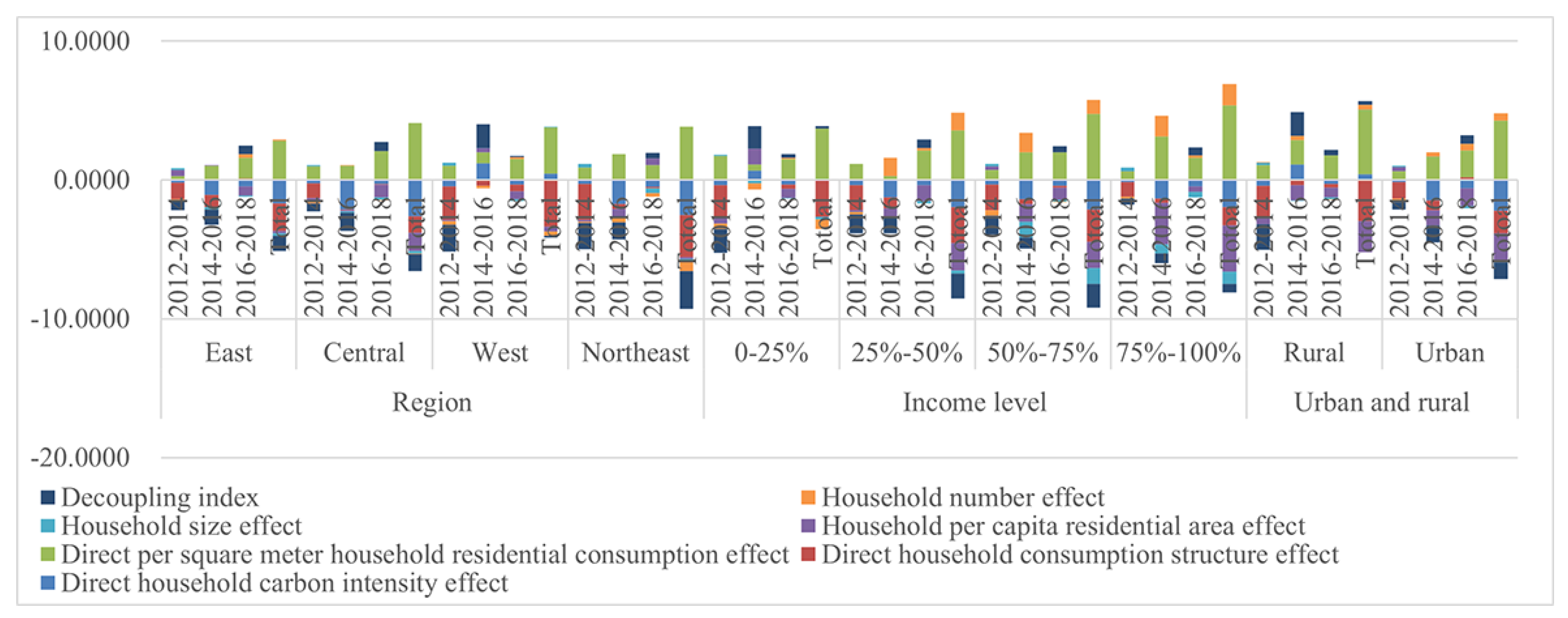
3.3. Analysis of Driving Factors of Green Transformation of HCPs

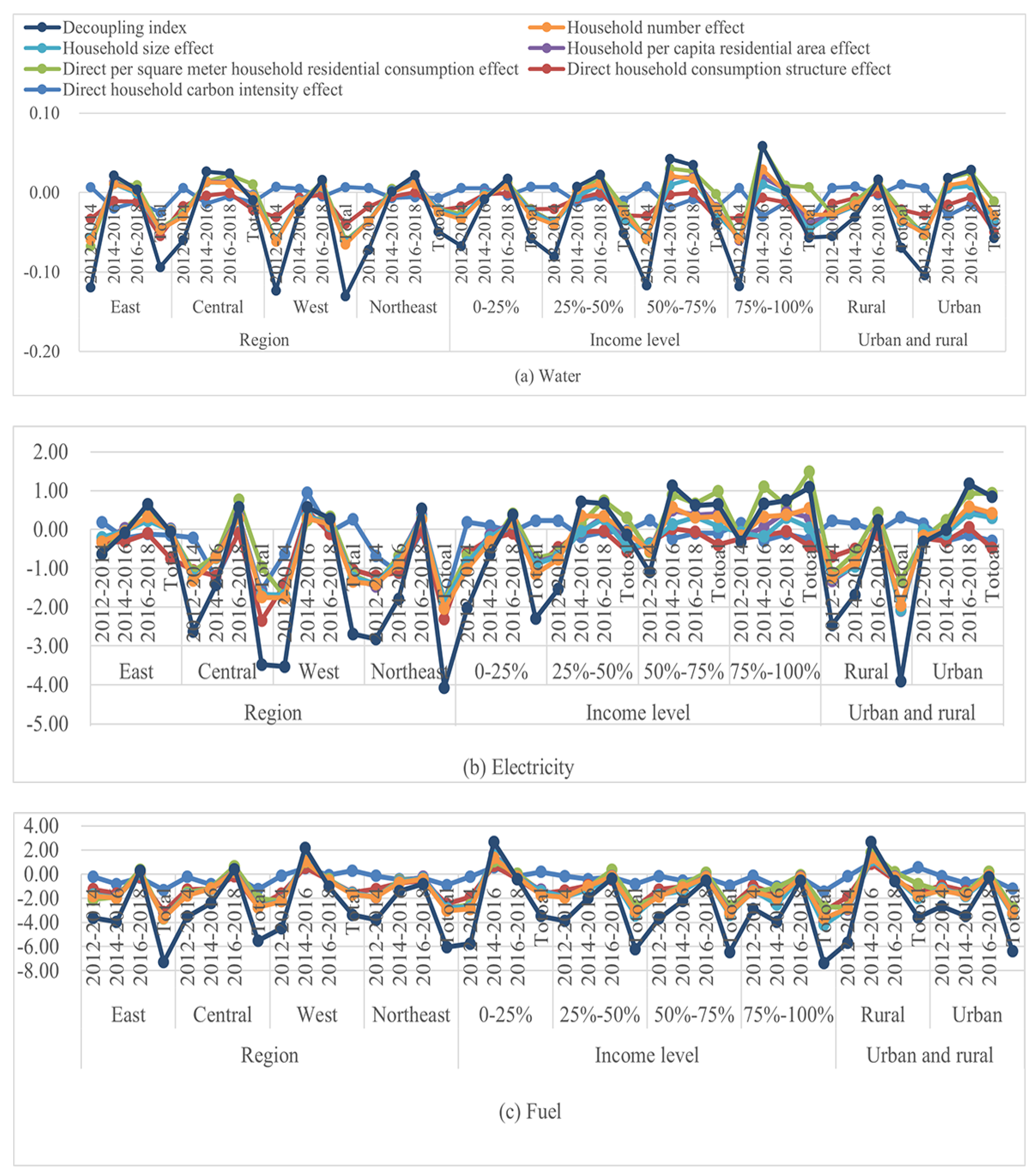
(1) Analysis of driving factors of green transformation of direct HCPs

According to Equation (7), driving factors of green transformation of direct HCPs and their four categories were analyzed from regional, income, and urban–rural perspectives.

In terms of driving factors of green transformation of direct HCPs within regions, income levels, and urban–rural areas, according to Figure 10, direct household carbon intensity exhibited a promoting effect from virtually all perspectives, indicating that it promoted the green transformation of HCPs. However, the western region, low-income groups, and rural areas exhibited an inhibitory effect, because the household energy structure in these perspectives had not been significantly improved and still relied heavily on coal.

The direct household consumption structure effect was negative, indicating its positive role in promoting green transformation of direct HCPs. This could be attributed to the increasing use of clean energy sources, particularly electricity, and the optimization of household energy consumption structure, which supported the green transformation of direct HCPs.

The direct per square meter household residential consumption effect was positive, indicating its inhibitory effect on the green transformation of direct HCPs. This could be attributed to the implementation of the 13th Five-Year Plan for Geothermal Energy Development and Utilization, issued by the National Development and Reform Commission, which resulted in higher HCEs from residential energy consumption.

The per capita residential area effect was negative, indicating its promoting role in the green transformation of direct HCPs. In general, an increase in per capita residential area led to a rise in HCEs when all other factors held constant. However, due to technological advancements in the construction industry, such as improved insulation and energy-efficient systems, energy consumption in heating and cooling has been significantly reduced. Consequently, the reduction in HCEs resulting from these technological innovations surpassed the increase in HCEs caused by the expansion of per capita residential area. Additionally, the growing awareness and adoption of green education principles encouraged residents to adopt eco-friendly habits, such as practicing energy conservation and engaging in sustainable consumption, which contributed to a decrease in HCEs.

Excluding western and northeastern regions and rural areas, the household size effect was negative, indicating its promoting role in the green transformation of direct HCPs. The trend of late marriage and late childbearing among contemporary young people resulted in smaller household sizes and a reduction in HCEs. However, the inhibitory effect observed in the western and northeastern regions and rural areas could be attributed to the population influx resulting from various strategies such as western development, northeast revitalization, and rural revitalization, which have led to larger household sizes and an increase in HCEs.

Excluding the central, western, and northeastern regions, and low-income groups, the effect of household number was positive, suggesting an inhibitory effect on the green transformation of direct HCPs. The increase in household numbers promoted HCEs. Therefore, the smaller household numbers in the central, western, and northeastern regions and among low-income groups caused lower HCEs.

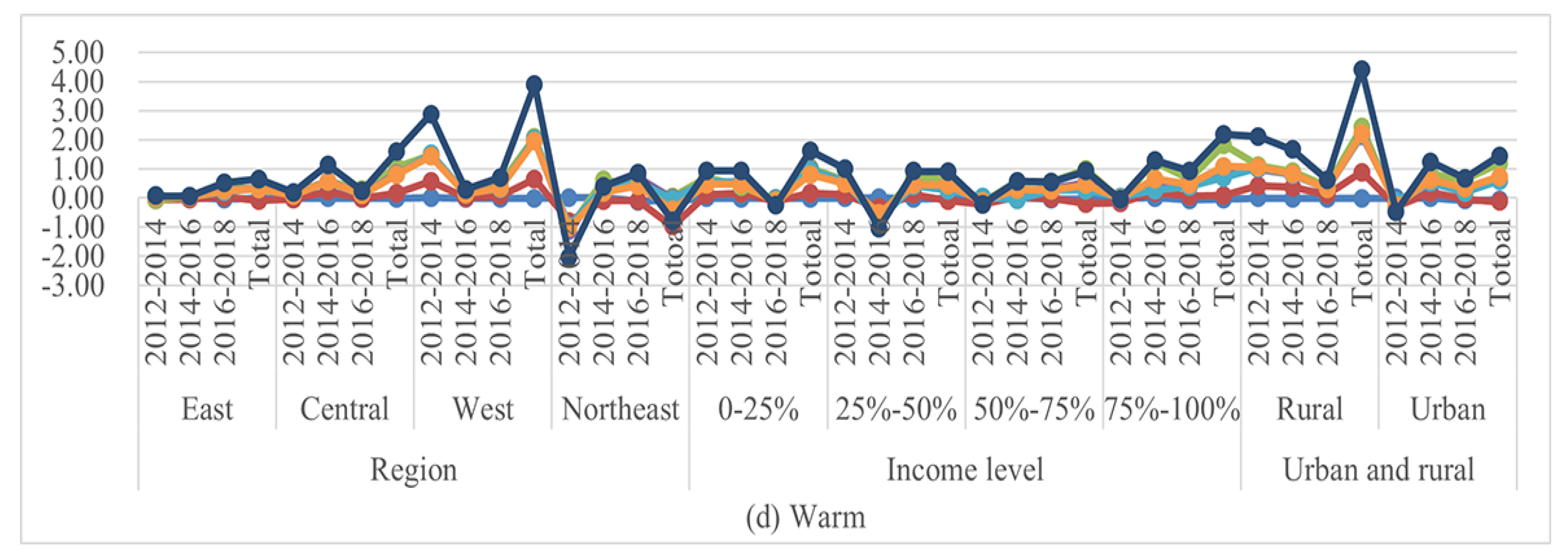
In terms of driving factors of green transformation in the four categories of direct HCPs, according to Figure 11, both direct household carbon intensity and household size hindered the green transformation of the four categories of direct HCPs from 2012 to 2014 but promoted it from 2014 to 2018. Direct household consumption structure promoted the green transformation of water from 2012 to 2014 but inhibited it from 2014 to 2018. Furthermore, the direct household consumption structure primarily promoted the green transformation of electricity and fuel but inhibited that of warm. Direct per square meter household residential consumption promoted the green transformation of water and electricity from 2012 to 2014 but inhibited it from 2014 to 2018. Similarly, direct per square meter household residential consumption promoted the green transformation of fuel from 2012 to 2016 but hindered it from 2016 to 2018. Moreover, the direct household per square meter residential consumption effect was consistent with the decoupling state of direct HCPs, indicating its primary role in the green transformation of direct HCPs. Household per capita residential area consistently promoted the green transformation of direct HCPs, while the effect of household number remained relatively insignificant and unstable.

(2) Analysis of driving factors of green transformation of indirect HCPs

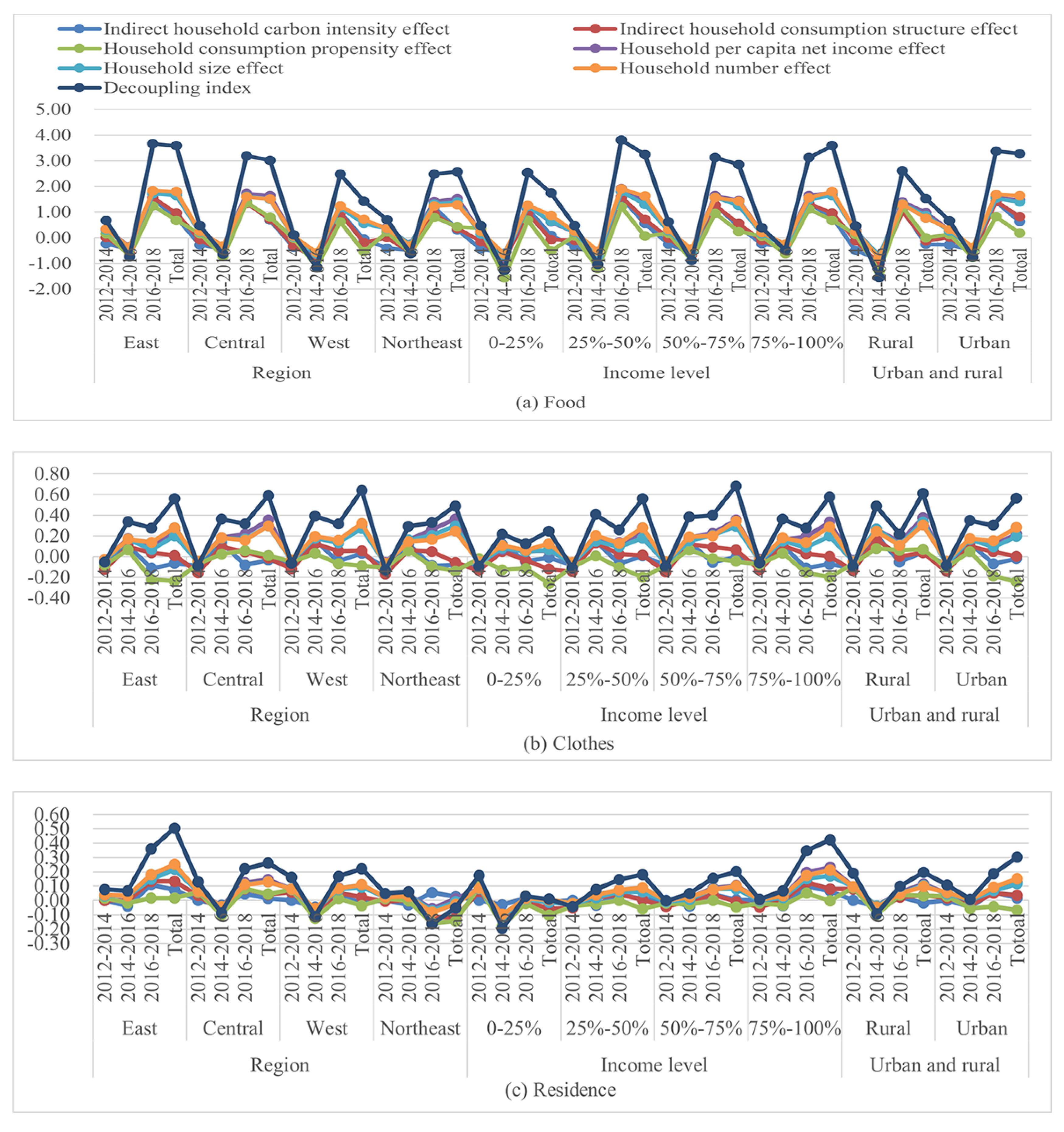
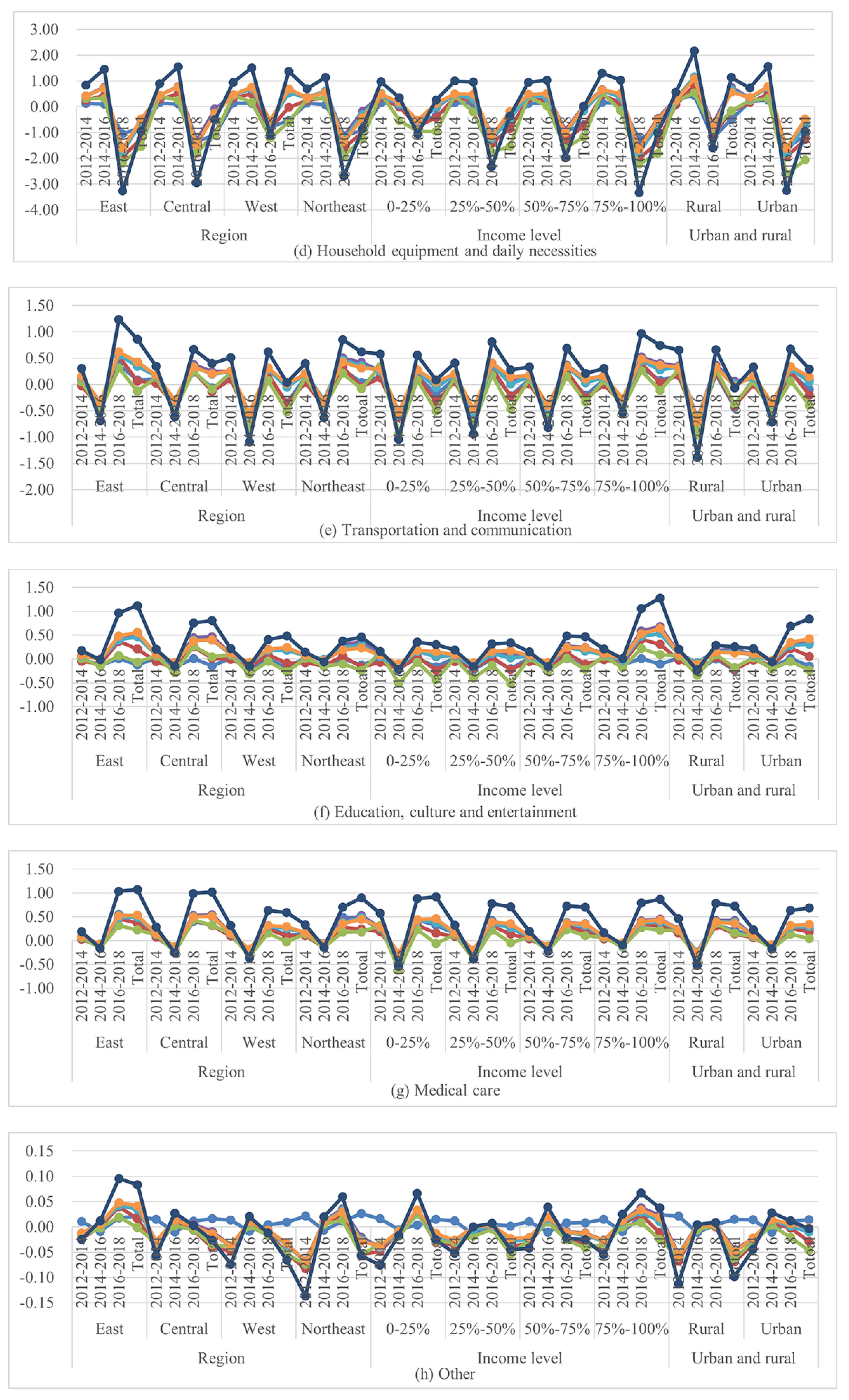
According to Equation (8), driving factors of green transformation of indirect HCPs including eight categories were analyzed from regional, income, and urban–rural perspectives.

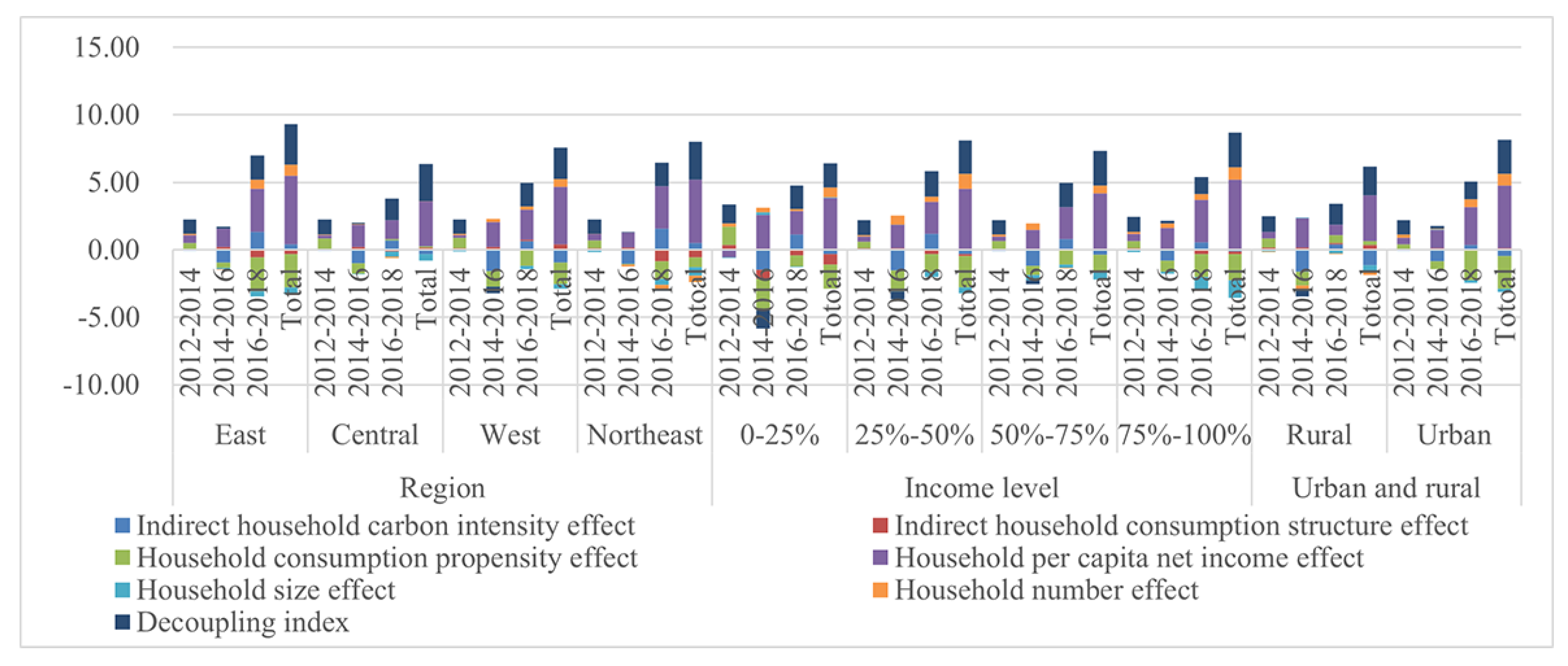
In terms of driving factors of green transformation of indirect HCPs within regions, income levels, and urban–rural areas, according to Figure 12, indirect household carbon intensity hindered the green transformation of indirect HCPs in the eastern and northeastern regions but promoted it in other regions. This could be attributed to the prevalence of products or services with higher EF of indirect HCPs in the eastern and northeastern regions.

Indirect household consumption structure hindered the green transformation of indirect HCPs in the central and western regions, high-middle-income groups, and urban–rural areas but promoted it from other perspectives. This could be attributed to the implementation of strategies like western development, new-type urbanization, and the rise of central China, which inevitably led to increased CEs while bringing benefits.

Household consumption propensity hindered the green transformation of indirect HCPs in the central region and rural areas but promoted it in other perspectives. This was because the central region and rural areas tend to consume products or services with higher EF.

Household per capita net income hindered the green transformation of indirect HCPs, which was because the increase in income tended to improve living conditions and increase the number of household appliances and private car ownership.

As household sizes increased, so did HCEs. Household sizes hindered the green transformation of indirect HCPs in low-income groups because of the increased demand for labor, which led to larger household sizes. However, the promoting effect in other perspectives was due to late marriage and childbirth, which reduced household size.

Household numbers promoted the green transformation of indirect HCPs in the northeastern region and rural areas. This could be attributed to urbanization and population outflow, which led to a decrease in household numbers.

In terms of driving factors of green transformation in eight categories of indirect HCPs, Figure 13 illustrates that the indirect carbon intensity effect aligned with the green transformation of eight categories of indirect HCPs. Per capita net income hindered the green transformation, while household sizes promoted it. Household consumption propensity hindered the green transformation of indirect HCPs from 2012 to 2014 but promoted it from 2014 to 2018. The effect of household number and household consumption structure on the green transformation of indirect HCPs appeared uncertain.

3.4. Marginal Effect Analysis

According to Equation (10), marginal effect analysis was conducted based on the main factors of green transformation of HCPs, i.e., residential area, household income, and household size, respectively.

(1) Marginal effect of residential area on HCEs

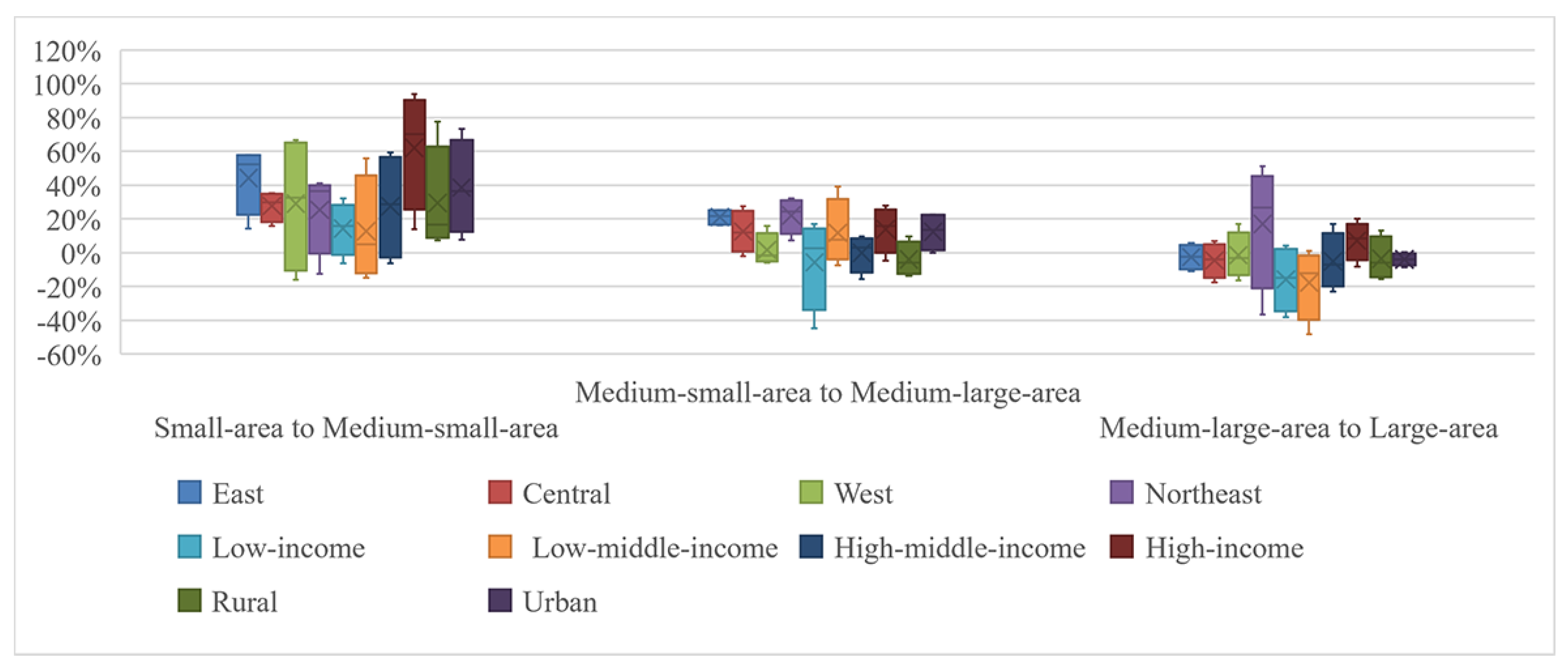
According to Figure 14, from 2012 to 2018, per capita HCEs varied across regions, income levels, and urban–rural areas as the residential area increased. In the eastern region, HCEs increased by 44.16%, 21.13%, and −2.50%. Central China saw increases of 27.75%, 12.48%, and −4.60%. Western China saw increases of 29.13%, 1.72%, and −1.40%. Northeast China saw increases of 25.40%, 22.15%, and 17.05%. In low-income groups, HCEs increased by 14.34%, −5.58%, and −15.74%. Low-middle-income groups experienced increases of 12.79%, 11.78%, and −17.70%. High-middle-income groups experienced increases of 27.48%, −0.10%, and −4.99%. High-income groups experienced increases of 62.12%, 13.86%, and 7.13%. In rural areas, HCEs increased by 29.43%, −3.84%, and −3.49%. Urban areas experienced increases of 38.61%, 12.46%, and −4.02%. The marginal effect of residential areas on per capita HCEs transformed from increase to decrease, from all perspectives. One possible explanation is that an increase in housing area signified an improvement in living standards and rapid economic development, which always go hand in hand with the development of more advanced energy-efficient and carbon-reducing residential construction technologies, as well as increased green consciousness education.

(2) Marginal effect of household income on HCEs

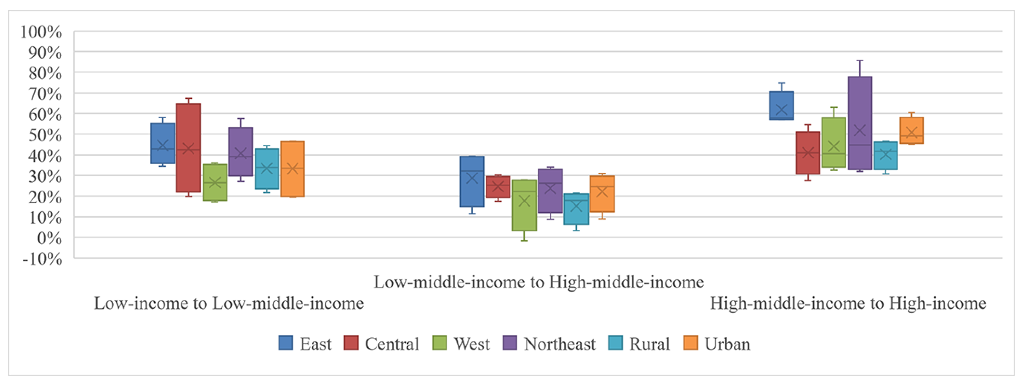
According to Figure 15, from 2012 to 2018, as household income increased, the per capita HCEs across regions and urban–rural areas varied. In the eastern region, HCEs increased by 44.62%, 28.78%, and 61.87%. Central China saw increases of 43.05%, 24.66%, and 41.00%. Western China experienced increases of 26.57%, 17.70%, and 44.10%. Northeast China witnessed increases of 40.72%, 23.78%, and 51.83%. Rural areas saw increases of 33.42%, 15.17%, and 40.23%. Urban areas saw increases of 33.30%, 22.22%, and 50.90%. Overall, the impact of household income on per capita HCEs increased across regions and urban–rural areas. During the transition from low income to low-middle income, residents strove to purchase essential household appliances and improved their living conditions, resulting in a significant increase in HCEs. However, during the shift from low-middle to high-middle income, the acquisition of previously unaffordable appliances led to a smaller increase in HCEs. As income level progressed from high-middle to high income, residents prioritized indulgent, service-oriented consumption and education, resulting in a rebound in the growth of HCEs.

(3) Marginal effect of household size on HCEs

The marginal effect of household size on HCEs was analyzed from direct and indirect perspectives.

In terms of the marginal effect of household size on direct HCEs, since the number of households larger than seven persons was too small, this study focused on analyzing samples of one to six persons. According to Figure 16, from 2012 to 2018, as household size gradually increased from one person to six, in the eastern region, HCEs increased by 62.59%, 29.92%, 9.89%, 18.58%, and 5.45%. The central region saw increases of 47.28%, 27.83%, 5.93%, 20.96%, and 2.75%. The increases in the western region were 43.80%, 20.90%, 9.86%, 15.76%, and 4.75%. The northeastern region saw increases of 32.24%, 14.04%, 3.21%, 2.25%, and 6.47%. Low-income groups experienced increases of 41.38%, 29.99%, 8.20%, 19.66%, and −3.70%. Low-middle-income groups saw increases of 33.01%, 18.78%, 11.50%, 10.25%, and 20.30%. High-middle-income groups exhibited increases of 53.93%, 18.19%, 5.87%, 15.72%, and 4.64%. High-income groups witnessed increases of 67.71%, 16.96%, 5.20%, 21.71%, and 12.25%. Rural areas saw increases of 45.07%, 25.54%, 7.40%, 18.46%, and 5.13%. Urban areas saw increases of 54.34%, 14.01%, 2.76%, 14.60%, and 5.78%. The marginal effect of household size on per capita direct HCEs decreased only when household size changed from five to six persons in low-income groups. The shift from a household size of one to two persons exhibited the highest increase in HCEs, while the transition from a household size of two to six persons showed a fluctuating decrease in the growth of HCEs. This could be attributed to the potential enlargement of living spaces as household size increased, resulting in an overall rise in HCEs. However, the shared utilization of resources such as water, electricity, fuel, and heating in larger households could significantly reduce HCEs.

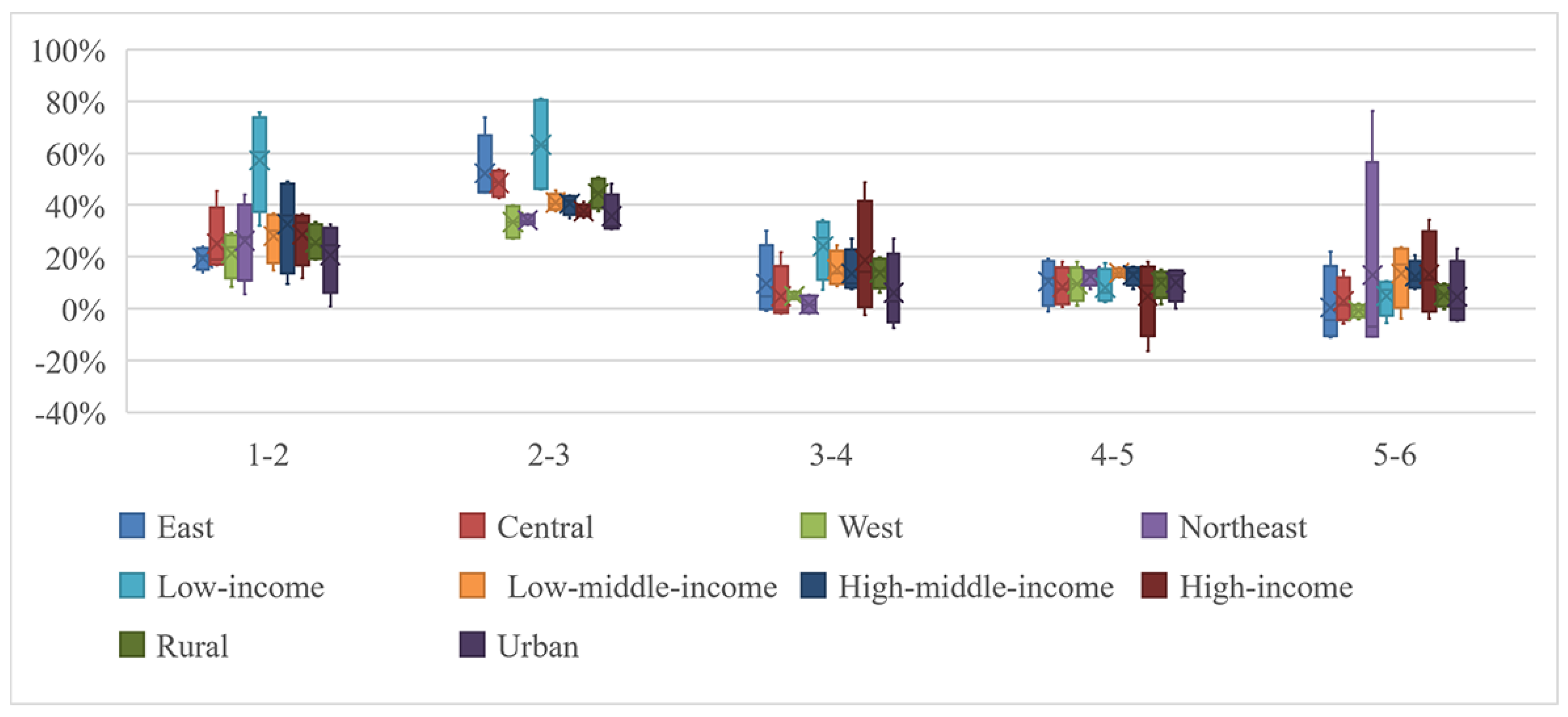
In terms of the marginal effect of household size on indirect HCEs, according to Figure 17, from 2012 to 2018, as household size increased from one to six persons, in eastern China, HCEs increased by 19.55%, 52.20%, 9.64%, 10.42%, and 0.40%, respectively. Central China experienced increases of 25.02%, 48.43%, 4.73%, 8.37%, and 2.95%. Western China saw increases of 21.24%, 33.37%, 4.88%, 9.50%, and −0.79%. Northeast China saw increases of 26.16%, 34.13%, 1.59%, 12.56%, and 12.90%. Low-income groups saw increases of 57.16%, 63.21%, 24.03%, 8.09%, and 4.92%. Low-middle income groups saw increases of 27.95%, 40.99%, 15.12%, 13.83%, and 13.44%. High-middle-income groups saw increases of 32.57%, 40.48%, 13.47%, 12.88%, and 12.43%. High-income groups experienced increases of 28.60%, 37.56%, 18.65%, 4.87%, and 13.22%. Rural areas saw increases of 25.53%, 44.46%, 13.80%, 9.98%, and 5.15%. Urban areas saw increases of 20.57%, 35.57%, 6.18%, 10.06%, and 4.62%. The marginal effect of household size on per capita indirect HCEs decreased only when household size changed from five to six persons in western China. The largest increases in HCEs were observed during the transition from a household size of one person to two and from two persons to three, highlighting the economies of scale within households, which suggests that compact family living is conducive to energy saving and carbon reduction. In households with three members, significant education expenses for children were incurred, while parents fostered emotional bonds through recreational facilities, leading to higher HCEs. However, households with a size of four to six persons had a population structure that included elderly individuals and pre-school children, who relied less on indulgent consumption, resulting in a reduced increase in HCEs.

4. Conclusions and Suggestions

This study aimed to explore the green transformation of HCPs and its driving factors, as well as propose practical and feasible recommendations. To achieve this goal, firstly, the study calculated the direct and indirect HCEs using the carbon emission coefficient method and the input-output consumer lifestyle approach, analyzed the characteristics of HCPs and HCEs, and identified the dominant types of HCPs. Secondly, the Tapio decoupling index method was employed to investigate the decoupling states between direct and indirect HCEs and HCEX, serving as an indicator of the degree of green transformation of HCPs. Subsequently, the LMDI decomposition method was used to analyze the driving factors of green transformation of direct and indirect HCPs. Finally, the marginal effect analysis was employed to further investigate the main driving factors of green transformation of HCPs. The following conclusions were drawn:

(1) From 2012 to 2018, the direct and indirect HCEX increased annually across regions, income levels, and urban-rural areas. However, the direct and indirect HCEs decreased in 2016. The primary contributors to direct HCEs were electricity and fuel, while indirect HCEs were primarily influenced by food, household equipment and daily necessities.

(2) In the measurement of green transformation of direct HCPs, all perspectives showed strong negative decoupling from 2012 to 2014 and weak decoupling from 2016 to 2018, but the decoupling state in 2014–2016 showed uncertainty.

Regarding the green transformation of four categories of direct HCPs, the decoupling states of four categories were unstable in different perspectives. Virtually all perspectives showed strong negative decoupling from 2012 to 2014 but fluctuated between strong and weak decoupling from 2016 to 2018.

(3) In the measurement of green transformation of indirect HCPs, all perspectives experienced expansionary negative decoupling in 2016–2018. However, the decoupling state in 2012–2016 showed uncertainty. Namely, virtually all perspectives showed expansionary linkage in 2012–2014 but showed strong and weak decoupling in 2014–2016.

Regarding the green transformation of eight categories of indirect HCPs, strong and weak decoupling were commonly witnessed, but expansionary negative decoupling was witnessed for food from 2016 to 2018.

(4) The green transformation of direct HCPs can be analyzed in three ways. Firstly, in view of influence strength, per capita residential area and household size exerted the greatest impact. Secondly, in view of influencing direction, direct household consumption structure and per capita residential area presented promoting effects, but direct per square meter household residential consumption presented an inhibiting effect. Thirdly, the effects of household number, household size, and direct household carbon intensity on the green transformation of direct HCPs showed uncertainty from all perspectives.

Regarding the green transformation of the four categories of direct HCPs, the direct per square meter household residential consumption effect aligned with the green transformation of the four categories. In view of influencing direction, the effect of direct household carbon intensity and household size on green transformation of the four categories of direct HCPs changed from inhibition to promotion, while per capita residential area played a promoting role. Furthermore, the effect of direct household consumption structure, direct per square meter household residential consumption, and household number among the four categories showed uncertainty.

(5) The green transformation of indirect HCPs can be analyzed in two ways. Firstly, in view of influence strength and direction, per capita net income exerted the most inhibitory effect. Secondly, the effects of other factors from each perspective were uncertain. Indirect household carbon intensity, indirect household consumption structure, household consumption propensity, and household size promoted the green transformation of indirect HCPs from virtually all perspectives; among them, household size exerted the largest promoting effect, while household numbers presented an inhibiting effect from virtually all perspectives.

Regarding the green transformation of eight categories of indirect HCPs, indirect household carbon intensity was aligned with the green transformation of the eight categories of indirect HCPs. In view of influencing direction, per capita net income and household numbers presented an inhibiting effect, while household size played a promoting role. The effect of household consumption propensity transitioned from inhibition to promotion. Furthermore, the effects of indirect household carbon intensity and indirect household consumption structure among the eight categories were uncertain.

(6) From all perspectives, the marginal effect of residential areas on per capita HCEs presented a trend of increasing to decreasing. The marginal effect of household income on per capita HCEs consistently increased. Similarly, the marginal effect of household size on per capita HCEs increased, but it decreased in low-income groups and in the western region when household size increased from five to six persons. The largest increases in HCEs were observed when household size changed from one to two persons and from two to three persons.

The following suggestions are proposed based on the findings. The green transformation paths of HCPs in regions, income levels, and urban–rural areas are shown in

Table 3. Green transformation paths of HCPs among regions, income levels, and urban–rural areas.

Influencing Factor	Improving Path	Regions, Income Levels, Urban-Rural Areas
Direct household carbon intensity	Promote technological innovation	West, low income, rural
Indirect household carbon intensity	Promote technological innovation	East, northeast
Indirect household consumption structure	Improve household consumption structure	East, west, urban
Direct per square meter household residential consumption	Improve the utilization of living space	East, central, west, northeast, low income, low-middle income, high-middle income, high income, rural, urban
Household consumption propensity	Encourage green consumption in households	Central, rural
Household per capita net income	Guide green consumption	East, central, west, northeast, low income, low-middle income, high-middle income, high income, rural, urban
Household size	Prevent household downsizing	West, northeast, low income, rural
Household number	Promote emigration	East, low-middle income, high-middle income, high income, urban

.

Promote technological innovation: It is recommended that the manufacturing industry allocate greater resources to scientific research and development. Promoting technological innovation and progress in production processes for products required by households is crucial in mitigating the inhibitory effect of household carbon intensity on the green transformation of HCPs.

Improve household consumption structure: It is imperative to decrease dependency on energy generation from fossil fuels and enhance the availability of clean energy sources like hydropower, nuclear power, and wind power in order to optimize household consumption structure. Additionally, efforts should be made to enhance the efficiency of conventional power generation and energy supply enterprises to minimize energy loss during transportation.

Improve the utilization of living space: It is crucial to enhance the utilization rate of living spaces, improve the quality of energy transmission, and ensure a rational distribution of residential buildings, which can be achieved through the establishment of green and low-carbon communities, optimization of layouts for living space, promotion of energy sharing, and enhancement of energy efficiency in households.

Encourage green consumption: It is important to encourage green consumption practices and promote the adoption of healthy and low-carbon behaviors among residents, which can be achieved by providing subsidies to incentivize households to purchase highly energy-efficient appliances and new energy-efficient vehicles, and offering citizens convenient and diverse low-carbon transportation options.

Guide green consumption: It is crucial to promote green consumption and encourage the adoption of environmentally friendly products. The marginal effect analysis revealed a significant increase in HCEs when transitioning from low to low-middle income and from high-middle income to high income. Therefore, governments should focus on guiding the high-middle-income groups towards greener HCPs while educating households about sustainable consumption patterns. The rise in household per capita net income has increased the demand for durable items like cars, air conditioners, and refrigerators, which has led to increased energy consumption in oil, electricity, and coal, resulting in greater HCEs. Thus, low-income households should be guided to improve their quality of life while reducing HCEs through green appliance subsidies and environmental conservation education.

Prevent household downsizing: Marginal effect analysis revealed that smaller households tended to produce greater per capita HCEs. Thus, it is necessary to encourage young individuals to enter into marriage and furthermore to implement policies like the two-child or three-child policies and establish strict divorce procedures to decrease the divorce rate.

Promote emigration: Initiatives should be taken to transfer or shut down enterprises and industries with high pollution and energy consumption in order to address the impact of household numbers on HCEs. Simultaneously, efforts should be made to improve employment opportunities and social service facilities in surrounding areas and promote the outflow of households from densely populated areas to prevent excessive population density and congestion from contributing to increased HCEs.

5. Research Limitations and Future Directions

This study investigated the green transformation of HCPs and its driving factors from the perspective of HCEs. Based on empirical findings, several green transformation pathways for HCPs within the Chinese context are proposed. However, there is room for improvement in the empirical design, and future research should consider the following two points:

(1) This study investigated the green transformation of HCPs and its influencing factors from regional, income, and urban–rural perspectives. Marginal effect analysis was conducted on the main influencing factors. However, this study failed to consider the influence of household characteristics on the green transformation of HCPs from these perspectives. Gender, educational level, marital status, and age structure might also affect the green transformation of HCPs. Future research could focus on the impact of household characteristics on the green transformation of HCPs to enhance the objectivity and scientificity of the research results.

(2) This study investigated the green transformation of HCPs and its influencing factors from the perspective of CEs. Considering the current context of “dual carbon” targets in China, future research could investigate the phased impact of policy factors related to the “dual carbon” goals on the green transformation of HCPs. This would facilitate the provision of differentiated green transformation pathways tailored to different stages of development.