A Model for Spatially Explicit Landscape Configuration and Ecosystem Service Performance, ESMAX: Model Description and Explanation

Abstract

It is critical that we move our understanding of the ecosystem services (ESs) produced by landscapes from the present abundance of analysis to a fundamental basis of design. This involves enhancing the ability to understand and model the interconnected, coevolving system of humans and the rest of nature, thus contributing to the design of sustainable landscapes. In this paper, we hypothesise that the spatial configuration of landscape components (the size and arrangement of tree clumps, paddocks, crops, water features, etc.) impacts the production of regulating ESs, which in turn have a leveraging effect on provisioning and cultural ESs. Drawing on the precepts of Ecological Field Theory, we present the development and implications of a conceptual Geographic Information System (GIS)-based model, ESMAX, that utilises the idiosyncratic distance-decay characteristics of regulating ESs. These ‘ES fields’ are visualised as radiating into the landscape from their source components, addressing a gap in biophysical reality that has been identified as a shortcoming of existing ES modelling based on landcover proxies. Hypothetical landscape arrangements of simplified landscape components are tested with ESMAX across three regulating ESs: cooling effect, nitrogen retention, and habitat provision. The model calculates the overall ES performance of each landscape arrangement by tabulating the ES fields produced and, critically, the nonlinear response where fields overlap. The results indicate a primary sensitivity to the size of components and a secondary sensitivity to the arrangement of components. Consequently, ESMAX can be used to design landscape configurations that (1) maximise the production of specific regulating ESs and (2) improve the utilisation of natural ES-producing resources.

1. Introduction

The design of landscapes to maximise the performance of multiple ecosystem services (ESs), including food production, but also carbon storage, recreation, nutrient management, flood control, and disease regulation (to name a few), is an urgent scientific challenge [1,2]. This ability to understand and model the interconnected, coevolving system of humans and the rest of nature is of paramount importance to the design of sustainable landscapes [2,3] To develop this design knowledge requires testing. Carrying out real-world testing of landscape arrangements that optimise the supply of multiple ESs, at any scale, poses unrealistic experimental, technical and financial challenges. The alternative is to create purposeful virtual models of landscapes [4,5]. Such models, despite their simplified representation of real-world systems, can then be used to define problems, organise and communicate thoughts, integrate information and theories across multiple scales, make predictions, and test understanding and theories [6,7]. A number of models have been developed to analyse and calculate multiple ESs generated by landscapes [8,9]. Tools such as LUCI (Land Utilisation Capability Indicator), ARIES (Artificial Intelligence for Ecosystem Services), and InVEST (Integrated Valuation of Ecosystem Services and Trade-offs) allow quantification of ESs, based on maps where landcovers (such as patches of pasture, water features, or forest) are treated as proxies for the production of specific ESs from particular landscape components [9,10,11,12]. Such tools allow relationships to be inferred between the spatial configuration of these components and ES performance [13,14]. However, these proxy-based models overlook the biophysical interactions between the different landscape components included in the model; they focus only on what occurs within the spatial boundaries of the service-providing components [15,16]. Without an understanding of what drives interactions between components, our ability to proactively arrange landscape components to enhance ES performance is limited. This limits our capacity to move from diagnostic analysis to the proactive design of landscapes that deliver desired ES performance. A crucial knowledge gap is the absence of empirical research into these critical spatial relationships, which prevents spatial interactions between components from being realistically modelled. Therefore, the first essential step for the integration of spatial interactions between components into landscape-scale ES models is the development of conceptual models capable of mimicking the observed relationships between the spatial configuration of landscapes and their ES performance [7,17]. These models can then be used to make predictions about ES performance resulting from different sizes and arrangements of landscape components. This enables maximum utilisation of natural capital increasingly under spatial pressures brought on by urbanisation, land-use change, and the geographic impacts of climate changes, thus facilitating the spatial design of sustainable landscapes.

We hypothesise that adjustments in the size and spatial arrangement of landscape components influence the supply of ESs. The primary objective of the work reported here is to present the development and implications of a spatially explicit model, ESMAX. This conceptual model uses observed distance-decay phenomena particular to specific regulating ESs to visualise and quantify predicted ES performance resulting from various spatial configurations of landscape components. Regulating ESs are so called because they regulate the impacts of natural events or human activities [18]. Examples include maintenance of water quality (for human consumption and waterway biological health), climate regulation, provision of biodiverse habitat, and flood protection (both from riverine flooding and because of sea level rise). Critical to the design of multifunctional landscapes, regulating ESs also underpin the other two categories of ESs—provisioning ESs (the provision of water, food, and fibre) and cultural ESs (the cultural, emotional, and recreational value arising from our perception of ecosystems [19]) [20,21]. Our work extends the efforts of Mitchell et al. (2015) [22] and Laca (2021) [23], setting forth an understanding that a) the intensity of ESs supplied by an individual landscape component decays with distance from that component to the surrounding area, and b) that these distance-decay fields, or ‘ES fields’, respond in idiosyncratic ways (depending on the ES in question) when they overlap with ES fields from neighbouring components. The degree of amplification at this overlap is germane to the total ESs supplied by that landscape configuration and, we suggest, to a new spatial approach to ES-based design [23]. For illustrative purposes, we focus on the supply of three ESs—cooling effect, provision of avian habitat, and sub-surface nitrogen interception—being supplied by simplified woody vegetation components arranged in a variety of configurations across a hypothetical, neutral landscape. This is the first time the ES field concept has been applied and is intended to show the general applicability of this concept to any type of ES whose transmission is based on the flow of organisms, materials, and energy [24,25]. This conceptual approach fulfils a didactic function by expanding comprehension of hitherto invisible and unheeded spatial-ecological relationships between landscape components. A mathetic function is also fulfilled—a basis for learning through the application of the model and considering afresh the design implications of size and arrangement of landscape components on ES performance and, subsequently, landscape sustainability.

2. Materials and Methods

The ESMAX is a conceptual model based on the concept of ES fields, developed using a Geographic Information System (GIS) platform. The model proceeds in four steps: (1) the characteristic distance-decay specific to each ES is determined by a literature review; (2) GIS translates these distance-decay characteristics as visualisations of ES fields radiating from individual components; (3) various spatial configurations of components are created; and (4) GIS quantifies the total ESs provided by each configuration, based on the total area of ES fields and the response of ES performance when ES fields overlap.

2.1. Extending Ecological Field Theory

In this research, the individual landscape components supplying the ESs are termed service-providing units (SPUs), defined for our purposes as an assemblage of ecosystem processes and organisms that collectively provide a regulating ES [26,27,28]. The method we use to characterise the ES distance-decay from an SPU and its overlap responses with neighbouring ES fields is drawn from Ecological Field Theory [29,30], which quantifies the effect of an individual plant on its neighbours using geometric fields of influence radiating from individual plants. These plant–plant interactions are subject to (i) a first-order distance-decay field of influence that is characteristic of the source plant and (ii) a specific second-order interaction response when overlaps occur with the fields of neighbouring plants [31]. In our work, first-order effects are the expected ES values arising from individual SPUs; second-order effects reflect spatially dependent interactions between two or more SPUs—effects which have not previously been accounted for in ES modelling [32,33]. Laca (2021) has proposed one-dimensional Cartesian graphs (with the y-axis expressing ES intensity and x-axis the range that the ES extends from the SPU) to express the first-order effects of ES supply from SPUs at various scales in a rural landscape. The form of the resulting graph is designated as a characteristic ‘kernel’ for each regulating ES. Ecological Field Theory proposes that the overlap response of these kernels can be linear or nonlinear [31]. In translating Ecological Field Theory to our research, we speculate that the complex interaction of energy, organisms, and materials comprising the spatial flow of regulating ESs will result in nonlinear responses when they overlap [34,35,36,37]. We use GIS to translate and visualise the first-order one-dimensional kernels into two-dimensional ES fields radiating from their respective source SPUs. To account for second-order effects occurring wherever ES fields overlap, we then apply a GIS filter to these two-dimensional ES fields, applying an algebraic expression for the nonlinear response.

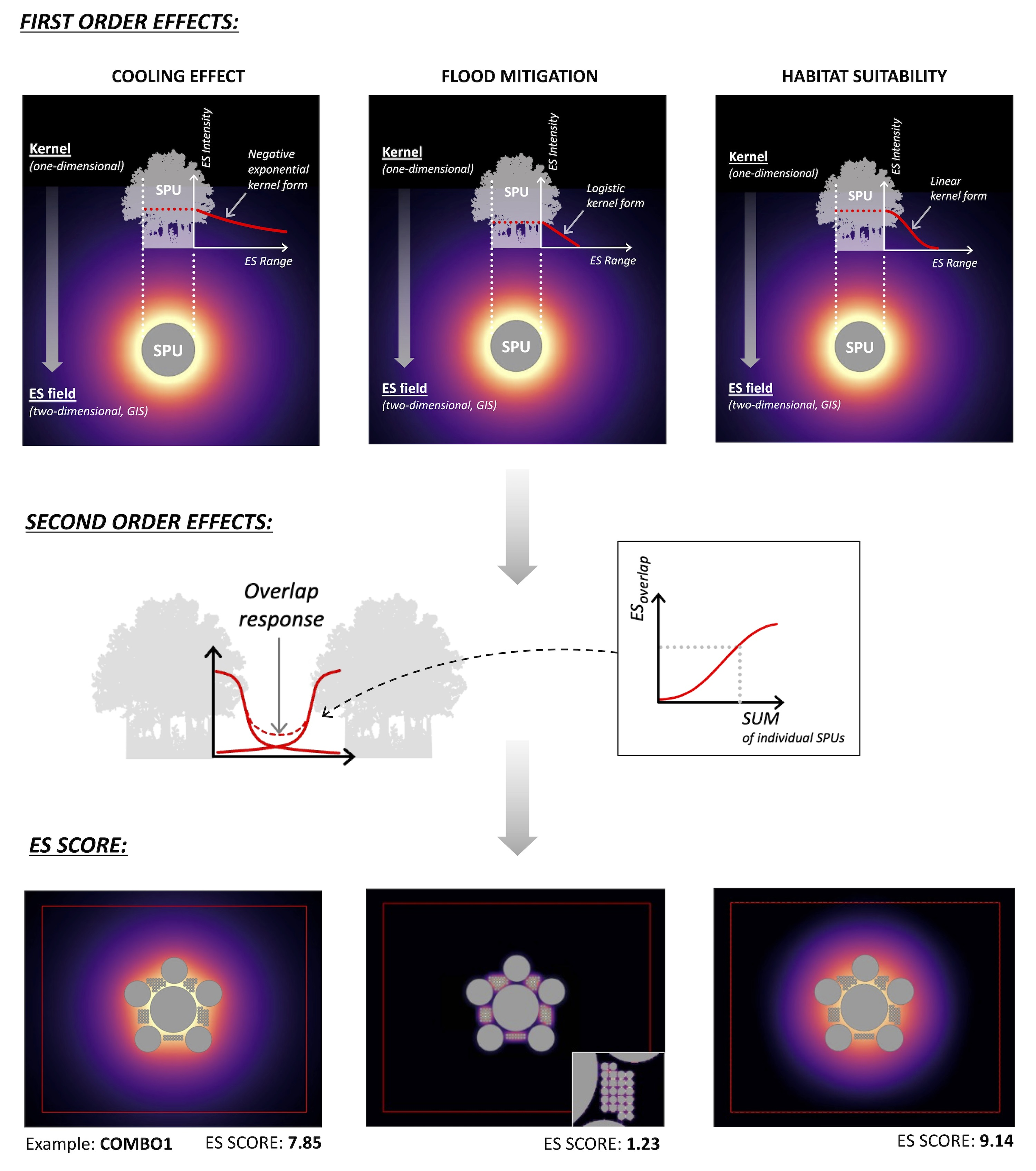
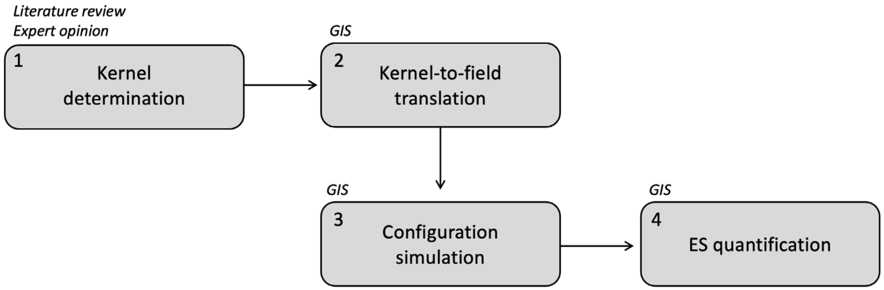
2.2. Model Structure

The structure of ESMAX is illustrated in Figure 1 and described in the following sections.

2.2.1. Step 1—Kernel Determination

The first step of ESMAX characterises the ES field particular to each ES. This determines the one-dimensional kernel that is then translated to a two-dimensional ES field in GIS. A literature review and expert opinion are used to determine the biophysical distance-decay characteristics of each regulating ES from its source SPU [33] (Figure 2a). 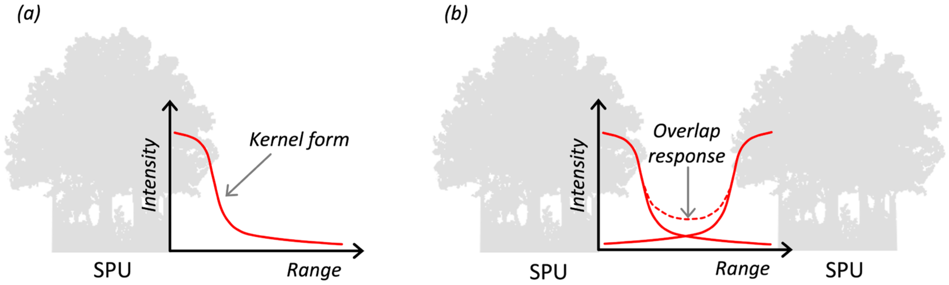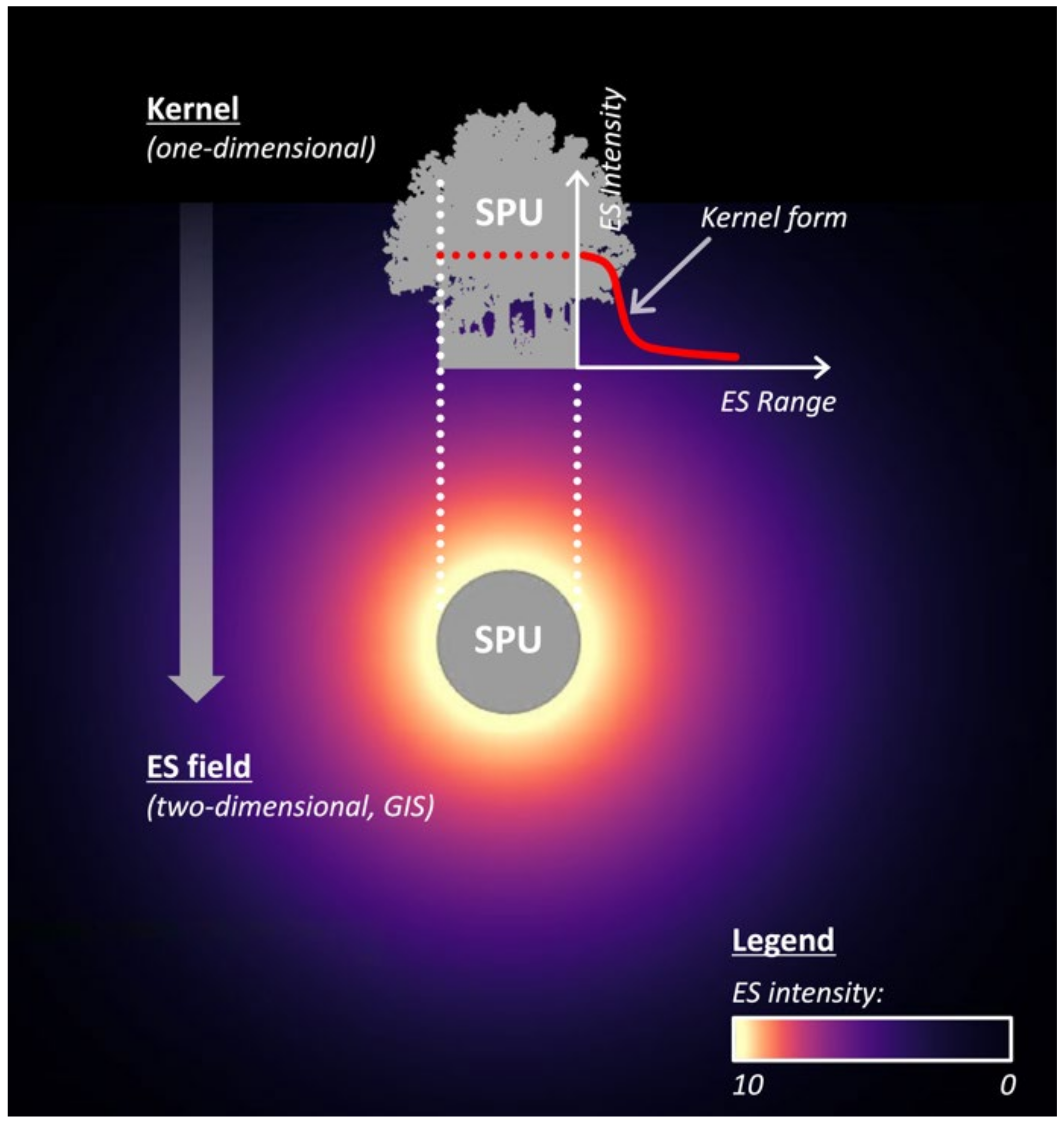The approach used to construct the kernel as a Cartesian graph followed the heuristic method set out by Ecological Field Theory to determine the four properties of the kernel—intensity, range, kernel form, and overlap response [29]. The first three of these properties define the first-order effects associated with individual SPUs; the fourth property, overlap response, defines the second-order effects arising when the ES fields of two or more SPUs overlap [32,33].

Intensity

Intensity is the amount of ESs supplied per unit area as a function of distance to the perimeter of the SPU. For this research, we utilise the approach taken by Mitchell et al. (2015), in which the distance-decay of the ES field commences at the SPU perimeter, from the highest possible intensity value, and we assume that ES intensity is constant across the SPU [22]. For the purposes of this model, within-patch heterogeneity was ignored [24], and the SPUs were assigned a homogeneous nominal landcover class to represent their woody vegetation composition. We emphasise that we are primarily interested in effects outside the SPU caused by interactions with other SPUs. Intensity therefore has a maximum when the distance from the SPU edge = 0 and usually declines with increasing distance from the SPU. Intensity is represented on the vertical axis of the kernel. Each ES is expressed in its own units, which are different for each ES.

Range

Range is the distance from the perimeter of the SPU over which the supplied ES decays and is represented by the horizontal axis of the kernel. In Ecological Field Theory, this distance depends on the physical size of the plant [29], whereas for ESs, the relationship between SPU size and ES range is contingent on the ES being assessed, as detailed below.

Kernel Form

The kernel form is the shape of the distance-decay characteristic of the ES, of which there are linear and nonlinear examples. Examples used to support Ecological Field Theory posit a linear distance-decay of plant influence on its neighbours from the centre of its stem/trunk [29]. With regard to ESs, Mitchell et al. (2015) infer that distance-decay can assume logistic or exponential form [22], depending on the ES being assessed. The distance-decay characteristics of ESs are not covered as explicitly in the literature as intensity and range. A general mathematical form representing the distance-decay characteristic of each ES was deduced from the literature review: Zardo et al. (2017) for the spatial characteristics of cooling phenomena associated with urban trees and parks, applied here as a basis to investigate rural cooling effect [38]; Laca (2021) for the spatial distribution of bird and insect populations within their habitat according to feeding and nesting behaviour [23]; and Philips et al. (2011) for tree root architecture relating to nitrogen retention [39].

Overlap Response

Overlap response describes the interaction between ES fields from neighbouring SPUs and is fundamental to the ES performance of a particular landscape configuration (Figure 2b). Depending on the ES being assessed, this second-order effect can range between two extremes: (1) additive, when the ES at any point is the sum of the overlapping fields, and (2) exclusive, when the ES at any point is the maximum individual value of the overlapping fields at that point [23]. A variety of biophysical processes and mechanisms can be involved in determining the amount of ESs provided when ES fields overlap. This work treats these as a ‘black box’ and focuses on the consequences of the overlap and resulting ESs produced. These overlap responses may be simple or complex, depending on the ES involved, but for the purposes of this initial development of the model, we assume the overlap response for each ES to be nonlinear. We assume that in overlap scenarios, each ES (i) exhibits a threshold and saturation phenomena, and (ii) the combination of overlapping ES fields can be represented by a nonlinear, sigmoid relationship [40]. We employ a basic logistic function:

$${\mathrm{E}\mathrm{S}}_{\mathrm{p}\mathrm{o}\mathrm{i}\mathrm{n}\mathrm{t}}=\frac{{\mathsf{\theta }}_1}{{\mathrm{e}}^{{(\mathsf{\theta }}_2-\mathrm{S}\mathrm{U}\mathrm{M})/{\mathsf{\theta }}_3}}$$

(1)

where ES_point = total ES intensity at a specific point, including second-order effects, SUM = sum of first-order ES values at a specific point contributed by each SPU kernel, θ₁ = asymptote (the nominal highest possible ES intensity), θ₂ = the value of the function’s midpoint (at which half the θ₁ value is reached), and θ₃ = the logistic growth rate or steepness of the curve.

We consider this function as a ‘filter’ and apply it to the sum of first-order ES values contributed by each SPU kernel at a specific point to simulate the total ESs produced in areas of overlap. Although it is premature to suggest that this function will hold in all real-world situations, we suggest that this approach provides a point of departure for hypotheses to be tested in empirical studies.

2.2.2. Step 2—Kernel-to-ES Field Translation

The second step of the ESMAX model uses GIS to visualise the ES field for each regulating ES. The one-dimensional kernel specific to each ES is translated algebraically into two-dimensional pixel-based ES fields (Figure 3), radiating isotropically from circular SPUs. This process is carried out using ArcGIS Pro (Version 3.0.1, Esri, Redlands, CA, USA) and involves the creation of a script based on ArcGIS Pro tools, allowing flexible inputs of both first-order distance-decay and second-order overlap parameters. Further details of the GIS tools used and their modifications are provided in the Supplementary Materials.

2.2.3. Step 3—Configuration Simulation

To illustrate the effect that landscape spatial configuration has on ES supply, circular SPUs of three sizes are arranged in 24 different configurations across a hypothetical 200 ha site (Figure 4). Each SPU is composed of a generic and homogeneous woody vegetation landcover, with the total area of 18 ha of woody vegetation constant in each configuration. This scale was selected as a reasonable area in which spatial arrangements of SPUs would affect the landscape-scale performance of the three regulating ESs being studied [41,42,43]. In creating these configurations, we are primarily interested in the effect on overall, landscape-scale ES performance caused by both the distribution of SPUs and the interaction between ES fields from neighbouring SPUs. Accordingly, the configurations are generated specifically to explore the effect of SPU size and degree of aggregation of SPUs across the research site. Aggregation is an umbrella term used in Landscape Ecology to describe several closely related concepts, including dispersion, fragmentation, and isolation [44]. To limit the number of potential explanatory variables, ESMAX contains a number of simplifications:

• As the SPUs are circular shapes, the respective ES fields of the SPUs are isotropic radiating circles, meaning that ES distance-decay is constant in all possible directions from the centre of the SPU.
• A neutral background landscape is assumed, contributing no ESs and homogeneous in terms of land use, soil type, etc., without landscape features (such as watercourses).
• Each SPU is assumed to comprise species suitable for testing the ESs included in our conceptual model. Future research could add composition as a further explanatory variable.
• Seasonality is not considered, and we assume the trees to be at peak maturity. The context of this initial development of the ESMAX is mainly spatial—we acknowledge there is a temporal dimension to ES supply, but we consider it implicitly by using a hypothetical time period and resolution that permits the assumption that rates are constant.
• SPUs are limited to three sizes: 6 ha, 2 ha, and 0.02 ha (designated large—L, medium—M, and extra small—XS, respectively). These areas represent thresholds for the specific ES being assessed. For example, Meurk et al. (2006) establish a functional hierarchy of bird nesting/feeding patch sizes, which we adapt for use in this research [45]. These thresholds are detailed in Section 2.3.3 below.
• Setting the total SPU area to 18 ha allows straightforward, whole-number distribution of homogeneously sized SPUs, i.e., 3 × 6 ha, 9 × 2 ha, and 900 × 0.02 ha. ‘COMBO’ configurations are also generated, which combined the three SPU sizes, while still maintaining a total SPU area of 18 ha (Figure 4).

Figure 4. The 24 spatial configurations of SPU patches used in this research. Nomenclature as follows: L (6 ha), M (2 ha), XS (0.02 ha) = the size of SPU in arrangements comprised of equal-sized SPUs (3 × 6 ha, 9 × 2 ha, and 900 × 0.02 ha; total SPU area = 18 ha); suffixes 1–6 = gradations of aggregation (1 = most aggregated, 6 = least aggregated); COMBO = configurations comprising 1 × L, 5 × M, and 100 × XS SPUs (total SPU area = 18 ha).

Figure 4. The 24 spatial configurations of SPU patches used in this research. Nomenclature as follows: L (6 ha), M (2 ha), XS (0.02 ha) = the size of SPU in arrangements comprised of equal-sized SPUs (3 × 6 ha, 9 × 2 ha, and 900 × 0.02 ha; total SPU area = 18 ha); suffixes 1–6 = gradations of aggregation (1 = most aggregated, 6 = least aggregated); COMBO = configurations comprising 1 × L, 5 × M, and 100 × XS SPUs (total SPU area = 18 ha).

2.2.4. Step 4—Field Quantification

The fourth step quantifies the total regulating ES supplied for each configuration assessed. This accounts for the first-order ES fields radiating from respective SPUs and the second-order effects in areas where these fields overlap, after application of the filter equation described in Step Two above (Figure 5). GIS sums the resulting individual ES pixel values to give the total ESs supplied for each landscape configuration. The total ES value is then normalised by subtracting the lowest ES total of all the configurations, then dividing this by the overall range of values. By multiplying this value by ten, we arrive at the ‘ES Score’ for that configuration (with 10 assigned to the best-performing configuration). Please refer to the Supplementary Materials for further detail of the GIS tools used and modifications required.

2.3. Application to Specific ESs

The following section provides detail about the three regulating ESs selected for this work and explains how their biophysical characteristics were translated to kernels and ES fields for use in ESMAX.

2.3.1. Selection of ESs

The three regulating ESs are selected to illustrate the general applicability of our conceptual approach to regulating ESs. Cadenasso et al. (2003) highlight the flows of energy, materials, and organisms constituting regulating ESs as essential to ecological systems [24]. In ESMAX, the cooling effect of tree clumps is an example of energy flow, the interception of sub-surface nitrates by tree roots is an example of material transfer, and the habitat suitability for the species studied relates to the movement of organisms. In the following section, we detail the biophysical processes and functions for each ES and their translation to characteristic ES fields.

2.3.2. Cooling Effect

The cooling effects of green spaces in urban areas are well established [38,46,47], but the cooling effect of trees in a rural context has not been studied to the same extent. Tree clumps in open fields also have the potential to provide cooling by inducing vegetation breezes, where warmer air over the open field rises, reducing local air pressure and drawing the cooler sub-canopy air from within the tree clump into the open area [48,49]. Urban cooling research suggests a nonlinear relationship between SPU size and cooling, reporting a minimum threshold of 2 ha for a significant cooling effect, which increases rapidly as park size increases to 8 ha, at which point the effect levels off [38,50,51]. The M-size SPU used in this research was set at 2 ha to correspond to this threshold size. Solitary XS-size SPUs (0.02 ha) are excluded, unless they are closely aggregated to another SPU. We defined ‘closely’ to mean an SPU located within the XS-size SPU diameter of another SPU, which correlates to its cooling effect range (see below). Kernel properties for cooling effect are summarised as follows:

• For the purposes of this model, the correlation of cooling performance increasing with SPU size noted in the literature is reflected in the kernel range (d_cool) increasing proportionally to the SPU diameter [38].
• The range is calculated with reference to the literature on micrometeorological phenomena characteristic of forest edge contexts [52,53]. The displaced, cool sub-canopy air will travel the same distance (d_cool) as the diameter of the source SPU. This assumption is supported by urban cooling research, which notes a cooling influence range of one park width away from the cooling source park [50,54].
• The kernel form is determined using the negative exponential distance-decay used in the InVEST (Integrated Valuation of Ecosystem Services and Trade-offs) urban cooling model [10].
• Overlap intensity of cooling effect is poorly understood. Our model ESMAX assumes that the overlapping of cooling fields will follow the same principle as the nonlinear amplification of temperature between two heat sources [55].

Further detail on the determination of cooling effect kernel properties in ESMAX are provided in the Supplementary Materials.

Assumptions and limitations: First, isotropic/anisotropic conditions in ESMAX do not account for local wind conditions. Both wind velocity and direction would have an impact on d_cool [56,57,58]. Second, the ES intensity is assumed to be constant, as noted above. Third, SPU composition is not considered in this research, and a constant value for cooling intensity based on evapotranspiration, albedo, and shading values is used [38].

2.3.3. Habitat Suitability

The connection between biodiversity and resilience of ESs—regulating, cultural, and provisioning—is well established [59,60,61,62]. The widespread loss of landscape spatial heterogeneity associated with intensive, monocultural agriculture is often viewed as a key driver of biodiversity loss in rural landscapes [63,64]. Repairing and sustaining biodiversity requires protection of remnant forest fragments, creation of new forest fragments, and the connection of these ecological systems across landscapes [65,66]. In this research, woody vegetation SPUs represent such forest fragments (reiterating that for the purpose of this conceptual model, species composition is not considered, and it is assumed SPUs are composed of species conducive to the particular ES being assessed). The relationship between biodiversity and spatial configuration of SPUs is supported by the island biogeography theory, whereby species diversity is a function of landscape fragment area and the degree of isolation [67,68]. Meurk et al. (2006) created a prescriptive and spatially explicit interpretation of island biogeography, proposing optimum reserve sizes and spatial configuration guidelines to enhance connectivity for indigenous flora and fauna in the human-modified landscapes of New Zealand [45,69]. These guidelines informed the SPU sizes used in this research:

• SPUs of 6 ha approximate a minimum core habitat area of 2.5 ha (once a perimeter buffer to the SPU edge of around 50 m is established), suitable for sanctuaries in human-modified landscapes [45].
• SPUs of 2 ha provide habitat for most plants, lizards, insectivorous birds, and invertebrates and provide resource-rich ‘steppingstones’ for nectivorous birds [45].
• SPUs of 200 m² (0.02 ha) provide finer-grained steppingstones and feeding locations [45].

In this work, two bird species with differing feeding and nesting characteristics are used to study the impact of spatial configuration on habitat suitability. One species is an insectivore that prefers forest edge habitats; the other is a nectar-feeder that requires well-buffered, inner-forest environments to breed [70,71,72]. The insectivore has adapted successfully to landscape fragmentation [45,73] and feeds in close proximity to the tree line [74,75]. In contrast, the nectivore will occasionally fly long distances (greater than 500 m) to feed on preferred flowering species [76,77,78]. ESMAX can be initialised for any species’ feeding and nesting spatial characteristics. For these two particular species, we used data obtained from the literature to generate an ES kernel for each species.

• Intensity, in this case, is a measure of feeding activity from a nesting base and was given an arbitrary maximum value. It is recognised that there is a minimum SPU area required for the establishment of nesting and establishment of a home range [45]. The insectivore will nest even in the smallest 0.02 ha SPUs (which translates to a 16 m diameter tree clump), as long as the distance to a neighbouring clump is no greater than 150 m [72]. Therefore, for the insectivore, intensity is set to zero in the smallest 0.02 ha SPUs if these were located more than 150 m away from other SPUs. For the nectivore, the minimum SPU area for nesting is set at 2 ha [79], and the intensity is set to zero in all 0.02 ha SPUs.
• Range (for feeding) is set at 100 m for the insectivore and 500 m for the nectivore.
• Kernel form is based on the triweight kernel used by Laca (2021), considered a reasonable representation of population distribution from a nesting site [23]. Its single parameter, λ, is the reciprocal of the range.
• ES overlap intensity is affected by territorial characteristics. The insectivore is noted to be territorial and will aggressively defend its territories from other members of the same species [80]. However, conspecific attraction of external individuals for breeding is demonstrated even in highly territorial species [81], so the overlapping fields are considered additive. The nectivore exhibits some territorial behaviour during the breeding season, but generally, feeding ranges may overlap [76,77,79]. The nonlinear logistic overlap response for both species reflects a negative density-dependent relationship, where population growth is curtailed by crowding, predators, and competition [82,83,84].

Assumptions and limitations: Included in the biotic and abiotic simplifications made for the purposes of this modelling is exclusion of the effects of predation and availability of food on the focal species. Our study refers to isolated populations of the studied species, and ESMAX assumes no changes in population. Interspecific and community processes are implicit and assumed as being constant over time.

2.3.4. Nitrogen Retention

Nitrogen retention, in this research, refers to the interception of sub-surface nitrates by the root systems of plants and trees [85,86,87]. Synthetic N fertiliser plays a significant role in most intensive agricultural systems and is frequently associated with negative impacts on environmental and human health [88,89,90]. The ES provided in this context is the prevention of excess nitrates from entering surface or ground water. The two main ecological mechanisms for the interception of sub-surface nitrate flow are uptake by vegetation and microbial denitrification [85,86,91]. Both processes are influenced by mycorrhizal activity occurring at the micrometre scale on root surfaces within the spatial extent of the rhizosphere of individual plants [92,93,94]. Therefore, this conceptual model transcribes the spatial distribution of root biomass as the kernel properties for nitrate retention [95]. Taking a reductionist approach, a linear approximation of root architecture is made, with root biomass (including both coarse and fine roots) concentrated towards the trunk, and the lateral extent of roots extending some distance beyond the crown diameter [96,97,98]. SPUs are defined by the above-ground extent of a tree clump (meaning the outer edge of the outermost tree trunks), and the kernel reflects the spatial distribution of roots for the outermost trees only. Kernel properties for nitrogen retention are summarised as follows:

• Maximum nitrate interception, the measure of ES intensity in this case, is given a constant arbitrary value.
• Range and kernel form are based on physical root spatial distribution measurements carried out in field research into the mechanical influence of trees on soil erosion [39,99,100]. We consider implicitly that there is some extension of ES range beyond the rhizosphere because nitrates move with water and by diffusion to volumes of lower concentration.
• We selected alder (Alnus viridis) as the focal species for this model, as it exhibited the greatest root biomass at the end of the field research referred to. This species exhibits a high degree of root interweaving [100], and we assume therefore nitrate interception capacity to be additive in areas of overlap. The rhizosphere is a vastly complex environment. For the purposes of this model, we base the additive nonlinear logistic overlap response on the following upper and lower asymptote assumptions: nutrient saturation establishes the upper asymptote [101,102,103] (i.e., maximum nitrate retention occurs closer to the root trunk), and root branching density decreasing further away from the trunk, lowering nitrate retention capacity, establishes the lower asymptote [104,105,106].

Please refer to the Supplementary Materials for further detail on determination of nitrate retention kernel properties.

Assumptions and limitations: ESMAX assumes uniform soils, uniform nitrate availability distributions, and symmetrical root biomass. In reality, soils are not uniform [39,107,108], root systems are often not symmetrically distributed [39,108], and nitrate availability is highly variable and too complex to be modelled accurately [109,110,111].

3. Results

ESMAX calculated the total pixel values of all simulated ES fields and areas of overlap to determine the overall ES performance of each spatial configuration. Figure 6 presents the ES scores for configurations ranked in order of size and degree of aggregation. From these results, it is noticeable that performance correlates firstly to SPU size and secondly to the spatial arrangement of SPUs in relation to each other. The relationship between SPU size and ES performance is highly dependent on the ES being considered. Figure 7 presents an illustration of ES fields radiating from individual SPUs in the configurations with the highest ES Score overall for each ES.

3.1. Result 1: Configuration (Size)

Generally, there is a stratification of ES production with configurations comprising mainly L-size clumps (6 ha) delivering a strong cooling effect, configurations dominated by M-size SPUs providing best nectivore habitat and configurations of mainly XS-size (0.02 ha) clumps providing strongest N retention and best habitat for the insectivorous bird studied. ESMAX results suggest the cooling effect is strongest in configurations that include the L-size woody vegetation SPUs, whether in arrangements featuring only that size SPU or in the arrangements comprising all sizes (Figure 7). This is a direct and expected result of the kernel for cooling, which is dominated by SPU size.

Configurations with M-size and COMBO SPUs provide the best habitat for the nectivorous bird. This is a combination of the 2 ha SPUs providing the minimum nesting habitat threshold for this species, and then being able to distribute this nesting area across the site to take most advantage of feeding range. Configurations dominated by XS-sized SPUs provided both the best habitat for the insectivorous bird species and nitrogen retention. This is explained by the relatively short range of these ESs (100 m feeding range for the insectivore and 7 m lateral root biomass extent for nitrogen retention), making them highly correlated to the high total of SPU perimeters in these arrangements. The magnified segments of the nitrogen retention images in Figure 7 show the ES field at close range (for diagrams showing the entire research area, the nitrogen retention ES field is practically invisible). Expressed another way, the more individual woody vegetation clumps in a landscape, the more nitrate was retained by root systems.

3.2. Result 2: Configuration (Aggregation)

Besides the clearly apparent relationship between size of SPUs and production of certain ESs, the results of ESMAX also reveal another level of correlation between ES performance and how SPUs are arranged in relation to each other. This is apparent across all the ESs studied here, noting that the difference in ES score resulting from changes in configuration are two orders of magnitude lower than the difference in ES score resulting from changes in size.

Across all size tiers, cooling performance increases with aggregation, i.e., the more clumped the SPUs were, the greater the net cooling effect. The results from ESMAX for the nectivorous species shows that arrangements with the M-size 2 ha SPUs tightly clustered are preferred, mimicking the species’ preference for intact bush habitat.

4. Discussion

The main objective of this work was to present a model that quantifies and visualises the difference in ES performance resulting from various spatial configurations of landscape components, and conceptually validating it through a series of simulations hypothesising that different spatial configurations of landscape components will produce different levels of ES supply. In comparison, existing models for analysing the ESs generated by landscapes use maps where landscape components (such as patches of pasture, water features, or forest) are treated as proxies for the production of specific ESs (Bagstad et al., 2013; Burkhard et al., 2014; Eigenbrod et al., 2010; Sharps et al., 2017) [9,12,112,113]. However, these proxy-based models, including LUCI, ARIES, and InVEST, overlook the biophysical interactions between the different landscape components; they focus only on what occurs within the rigidly defined spatial boundaries of the service-providing components (Lavorel et al., 2017; Seppelt et al., 2011) [15,16]. The conceptual approach of using circular forms to represent SPUs isolates the impact of configuration from other drivers of ESs, such as the component’s shape and composition. By simulating a range of spatial configurations, we were able to assess the effects of configuration and test the explanatory factors systematically. The results of the present modelling exercise provide a preliminary conceptual validation—as defined by Rykiel, 1996 [114]—of ESMAX’s capability to quantify ES performance at the landscape scale, as the model predicts/reproduce ES performance in a realistic manner and comparable to reports in the literature from real-world studies. Consequently, as a conceptual model, it is fit for purpose [7,114]. The results of the configurations tested align information about the spatial effects of urban cooling islands that we have transposed to a rural context [38], with the literature and expert opinion cited on insectivore nesting and feeding behaviour [72], and the interception of sub-surface nutrients in the rhizosphere [115]. We therefore argue that, within its context, ESMAX can be used with reasonable confidence to simulate and infer about real systems [114].

The output of ESMAX suggests that the spatial configuration of SPUs influences the supply of the three regulating ESs, thereby supporting our hypothesis. However, multiple simplifications and assumptions were made to develop this model. The next steps would be to upgrade the model so that it accounts for anisotropic site conditions such as soil type, topography and presence of landscape features, greater spatial and temporal complexity within the three ESs examined here, the incorporation of additional ESs, and the empirical testing of model outputs.

4.1. ES Field Theory: Addressing the Biophysical Gap

Several studies in the fields of ES Science and Landscape Ecology have proposed spatially explicit methods for the analysis of landscape multifunctionality [14,116,117]. As identified with regard to ES assessment tools using proxy-based maps, a major drawback of these approaches is that they overlook the so-called ‘biophysical gap’ [15]. This refers to a disconnect between the mapping of SPUs, usually represented as discretely bounded landscape features supplying a specific ES, and the reality of how biophysical processes generating these ESs invariably extend beyond these boundaries [118,119,120]. This disconnect inhibits better collaboration between ES Science and Landscape Ecology. ES Science generally works with proxy-based maps, taking an aerial view of the ES produced by isolated bounded SPUs [113,121]. In contrast, Landscape Ecology uses a more horizontal lens in attempting to understand the spatial interplay of landscape pattern and ecological functioning [2,122,123]. This horizontality is especially relevant to regulating ESs, which are dependent on lateral flows of energy, organisms, or matter [18,24,124]. The reality is that these lateral flows blur the boundaries of ecosystem patches, reflecting the dynamic complexity inherent in all ecological systems [125]. Engaging with the biophysical gap, by recognising, quantifying, and incorporating lateral biophysical characteristics, is therefore central to ES-based spatial design [13,22]. Our model adopts the hybrid approach suggested by Lavorel et al. (2017), retaining the use of proxy-based data (such as land-use/landcover mapping, which enables accessibility to a wide range of users), but incorporating the extension of biophysical activity beyond the SPU boundary through the second-order effects that occur when SPUs interact [22,37,68]. For example, the mechanics of the cooling effect model, while highly conceptualised for the purposes of this research, demonstrate that a cooling effect extends from an SPU into adjacent spaces. Previously, only the spatial distribution of shade in the context of rural cooling had been addressed [126]. While the cooling effect of evapotranspiration in rural contexts has been identified [127], ESMAX is the first attempt to spatially represent the cooling effect of woody vegetation, other than shading, in a rural context. This supports an additional layer of functionality for woody vegetation in agricultural contexts, significant to areas faced with increasing temperatures.

In relation to habitat suitability, ESMAX further develops the spatial configuration guidelines proposed by Meurk et al. (2006) by determining kernels for specific species and applying these characteristics to quantify and visualise the impact of habitat spatial configuration. It should be noted that Meurk et al.’s framework is not intended specifically for the two native bird species used in the model; it rather proposes a generic distribution of woody vegetation patches for the purpose of regenerating indigenous flora and fauna in Aotearoa New Zealand’s rural and urban landscapes. Their hypothesised spatial configurations are derived from tree establishment patterns resulting from wind and avian dispersal [45]. ESMAX’s enhancement of Meurk et al.’s framework maps these patches as discretely bounded SPUs, adding the distance-decay characteristics specific to the insectivore and nectivore studied, consequently advancing exploratory studies of spatial configuration to support biodiversity.

The kernel developed for N retention produces less obvious results in comparison to the other two ESs investigated due to the 7 m range of the ES field being barely visible at the scale used to illustrate the 200 ha research site. This result is not surprising, given most processes that involve plants and their soil involve movement over very small distances [23]. Nevertheless, ESMAX addresses the biophysical gap by recognising that the regulating ES effect of the clump extends beyond the obvious above-ground extents of the SPU. By visualising the effect of sub-surface ES fields, we can gain new insights into the arrangement of tree clumps to enhance sub-surface nitrate interception, and thereby potential retention.

Notwithstanding the visual limitations of the N ES fields when viewed at whole of landscape scale, for each of these three ESs, ESMAX generates a new graphical representation of spatial biophysical interrelations between landscape objects—the essence of the horizontality focussed on by Landscape Ecology. Comprehension of such unseen spatial effects is essential for an ES-based approach to design landscape interventions. Making biophysical functions explicit, here using a GIS-based approach, bridges a methodological gap between landscape configuration and ES production [112], and by extension, between Landscape Ecology and ES Science. For example, recent work by Cortinovis and Geneletti (2020) explicitly mapped and quantified ES supply and demand for the periurban context of Trento, Italy [128]. The regulating ESs studied—runoff mitigation, habitat provision, noise mitigation, air purification, and microclimate regulation (cooling)—were calculated based on strictly delineated boundaries of landcover data. Application of ESMAX to their process could be used to provide additional spatial information about the ES influence fields of respective ES sources. This would provide designers with important nuances in terms of quantity of ESs being supplied and the spatial distribution of these services.

4.2. Spatial Configuration and Implications for ES-Based Design

Mitchell et al. (2015) focus on the relationship between ES performance and spatial configuration from a conservation perspective, suggesting that managing patterns of natural landcover loss could help influence the provision of multiple ecosystem services in human-dominated landscapes [22]. Our interest in spatial configuration, on the other hand, is driven by the design of new landscapes, based on a holistic ecosystems approach, featuring new ecological networks characterised by multifunctionality and connectivity between patches [129]. Mitchell et al. (2015) incorporate the horizontal characteristics of a generic ES to conceptually model the spatial configuration of residual landcover fragments and resulting ES performance [22]. Our work extends this approach in two aspects. First, rather than presenting a generic ES, it proposes that distance-decay phenomena for specific individual regulating ESs can be decoded as a basis for engaging with spatial configurations. Second, where Mitchell et al. (2015) study the emission of a generic ES from a single SPU, our work draws on Ecological Field Theory to understand the cumulative effect of multiple ES sources. Supporting the premise that the capacity of a landscape to supply regulating ESs depends on the configuration of SPUs, our results suggest that different configurations benefit the three regulating ESs differently [14,18]. This creates opportunities for both spatial efficiency (supplying more ESs with less space) and spatial dexterity (inserting, manoeuvring, and coordinating multiple SPUs within a spatially constrained system). Understanding the way SPU size and spatial arrangement impact ES performance becomes especially relevant with interventions into occupied landscapes, as opposed to the hypothetical blank slate used in this paper. For example, the cooling effect model shows clearly that landscapes with configurations comprising solely L-size clumps deliver the greatest ES performance. These findings align with urban cooling research, recalling the observed increase in cooling effect of urban green spaces between 2 ha and 8 ha. However, the ESMAX output does not agree with (the very limited) research into the impact of spatial arrangement of urban parks on cooling. Lin and Lin (2016) modelled the effect of the spatial arrangement of urban parks (small, medium, and large sizes, based on a constant total combined area of 36 hectares) on cooling effect in Taipei. It should be noted their work only mentions ‘parks’ and makes no specific reference to trees. Their recommendation for optimal cooling effect was one large park and a regularly spaced distribution of small parks. The results reported by Lin and Lin (2016) do not align with our results, which emphasises the primacy of clump aggregation over dispersal. It is accepted that direct comparison between urban and rural contexts is limited by the built-up three-dimensional form of cities and the thermal differentials driven by highly contrasting urban surface materials [130]. Nevertheless, with further research into tree clump evapotranspiration, shade, and albedo effect, ESMAX could be developed and then provide guidance for the size and spatial arrangement of SPUs to deliver rural cooling effect most effectively. Practical application of ESMAX could include the expansion or agglomeration of existing stands of woody vegetation to enhance cooling effect. Dexterity, in this sense, also refers to spatial design to cool some parts of a landscape more than others, thus responding to context-specific demand for this ES.

Modelling habitat suitability with ESMAX assumes the objective of designing a biodiverse landscape in which both insectivores and nectivores thrive. While ESMAX allows for refinement of parameters to fit observed real-world behaviour of target species, designing for ideal habitat overlooks the ability of species to adapt to spatial arrangements at odds with an assumed ‘ideal’ habitat configuration. For example, the exclusion of XS clumps as habitat for the nectivore is slightly disingenuous, as they will feed on isolated trees of the preferred species [79]. What the graphs in Figure 6 demonstrate is the complexity involved with spatial-ecological interventions: even for two species of the same zoological order and not dissimilar allometry, the preferred habitats are significantly different. M-sized or larger SPUs are favoured by the nectivore, whereas the maximum forest edge provided by small SPUs is favoured by the insectivore, contributing another layer of complexity to the ‘right tree, right place’ adage [131,132]. ESMAX enables visualisation of this complexity, contributing to clearer ecosystem understanding by stakeholders and informing biodiversity-based decision making in a new way.

The ESMAX output for N retention, not surprisingly, shows greatest ES scores for the arrangements where the maximum overlap of ES fields occurs. In practical terms, this means the root systems of trees at the perimeter of adjacent SPUs are overlapping, thus increasing the root biomass density with which to absorb nitrates. The modelling of sub-surface N is extremely complex, with retention rates varying greatly under different land-use, climatic, and physico-geographical conditions [109]. To inform effective spatial design, understanding hydrological flows, and the impact that physical interventions have on these flows, is a starting point. As discussed earlier, ESMAX provides a visual understanding of the sub-surface retention being provided by root zones extending past the obvious above-ground perimeter of the tree clump. However, basing the ES fields solely on the physical extent of root biomass, without reference to sub-surface hydrological flow direction, means that the prosaic arrangement of woody vegetation clumps in close proximity to each other earns the highest ES scores (Figure 7). Development of modelling techniques that reveal the mitigated area downstream of SPUs is an area for future research. Establishing the ES field of the SPU beyond the physical extent of root biomass would allow ESMAX to test alternative configurations of woody vegetation SPUs in the landscape capable of providing high levels of N retention, rather than the axiomatic arrangement of clumps in close proximity to each other.

The evidence of different configurations of SPUs delivering different model outputs (or ES scores) underpins an ES-based spatial design approach and places ESMAX, in this initial development, as a proof-of-concept tool for this approach. Further aspects of ESMAX to be addressed include comparing the extent to which configuration affects ES performance with the impact of spatial composition (i.e., the various proportions of landcover types and species comprising each SPU), which is an important theme of current ES Science and Landscape Ecology discussion [14,116]. So too is the implication for spatial design of ES bundles (multiple ESs that tend to occur together synergistically according to specific spatial/temporal contexts and scales) [117]. The results of ESMAX also raise the important issue of identifying the correct scale for a particular intervention [124,133,134]. For example, both the habitat suitability and N retention models demonstrate connectivity being of paramount importance to the performance of both ESs. Yet, this connectivity occurs at very different scales: the degree of connectivity optimal for one ES is sub-optimal for the other. The spatial design of landscapes to deliver good performance in both habitat suitability for the insectivorous bird species and N retention would need to address this challenge. Such spatial trade-offs are at the crux of designing multifunctional landscapes, which is set out in the Introduction as the broader context of this research. Using the individual ES results of ESMAX to support the spatial design of multifunctional landscapes, in which a range of regulating ESs are supplied to match the local demand for these services, is a topic of ongoing research.

5. Conclusions

The model presented in this work, ESMAX, makes spatially explicit the ES fields of influence radiating from SPUs (in this case, woody vegetation clumps) in an agricultural landscape. ESMAX adapts existing theory on ecological fields to a) determine first-order distance-decay characteristics of single SPUs specific to certain regulating ESs and b) begin to comprehend the highly complex second-order effects on ES performance when ES fields from multiple SPUs overlap. By engaging with the biophysical gap in this way, ES fields can be graphically mapped. This has two benefits for Landscape Ecology and ES Science researchers in terms of designing sustainable landscapes. First, regulating ESs are, for the first time, visualised spatially. This is critical for supporting wider awareness of these essential, ‘pervasive and yet virtually unknown’ services. Second, the identification and quantification of ES fields, beyond the discrete boundaries of the SPU, point to a new, ES-based approach to spatial design.

With further parameterisation and testing, ESMAX could enable both Landscape Ecology and ES Science researchers by providing a common tool for more detailed, mechanistic research. Such development relies on parallel advances in the understanding of spatial implications of relevant ecological processes and functions. We suggest the ESMAX model has several features that facilitate this future development:

• The protocol for development of ES kernels, based on the Ecological Field Theory approach, is a simple iterative process and provides a ready platform for understanding the spatial implications of ecological functions.
• ESMAX is potentially applicable to a wide range of other flow-based regulating ESs, including air filtration, noise abatement, bioremediation, soil erosion control, flood protection, and pollination.
• The translation of kernels, specific to each ES, to a two-dimensional ES field is a novel use of basic GIS tools, which require minimal modification for this purpose.

This enhanced understanding of individual ESs will also assist future research into the influence of spatial configuration on multifunctional landscapes, in which a range of regulating ESs are supplied to match the local demand for these services.

References

- Bennett, E.M. Changing the agriculture and environment conversation. Nat. Ecol. Evol. 2017, 1, 18. [Google Scholar] [CrossRef] [PubMed]
- Wu, J. Landscape sustainability science (II): Core questions and key approaches. Landsc. Ecol. 2021, 36, 2453–2485. [Google Scholar] [CrossRef]
- Costanza, R. Valuing natural capital and ecosystem services toward the goals of efficiency, fairness, and sustainability. Ecosyst. Serv. 2020, 43, 101096. [Google Scholar] [CrossRef]
- Starfield, A.M.; Smith, K.A.; Bleloch, A.L. How to Model It: Problem Solving for the Computer Age; Burgess International Group: Edina, MN, USA, 1994. [Google Scholar]
- Groot, J.C.J.; Rossing, W.A.H. Model-aided learning for adaptive management of natural resources: An evolutionary design perspective. Methods Ecol. Evol. 2011, 2, 643–650. [Google Scholar] [CrossRef]
- Starfield, A.M. Building Models for Conservation and Wildlife Management; Macmillan: New York, NY, USA, 1986. [Google Scholar]
- Caswell, H. Theory and models in ecology: A different perspective. Ecol. Model. 1988, 43, 33–44. [Google Scholar] [CrossRef]
- Hamann, M.; Johnson, J.A.; Chaigneau, T.; Chaplin-Kramer, R.; Mandle, L.; Rieb, J.T. Ecosystem service modelling. In The Routledge Handbook of Research Methods for Social-Ecological Systems; Biggs, R.O., Ed.; Routledge: London, UK, 2021; pp. 426–439. [Google Scholar]
- Sharps, K.; Masante, D.; Thomas, A.; Jackson, B.; Redhead, J.; May, L.; Prosser, H.; Cosby, B.; Emmett, B.; Jones, L. Comparing strengths and weaknesses of three ecosystem services modelling tools in a diverse UK river catchment. Sci. Total. Environ. 2017, 584–585, 118–130. [Google Scholar] [CrossRef] [PubMed]
- Sharp, R.; Douglass, J.; Wolny, S. InVEST 3.10.2. User’s Guide; Stanford University: Stanford, CA, USA, 2020. [Google Scholar]
- Trodahl, M.I.; Jackson, B.M.; Deslippe, J.R.; Metherell, A.K. Investigating trade-offs between water quality and agricultural productivity using the Land Utilisation and Capability Indicator (LUCI)–A New Zealand application. Ecosyst. Serv. 2017, 26, 388–399. [Google Scholar] [CrossRef]
- Bagstad, K.J.; Johnson, G.W.; Voigt, B.; Villa, F. Spatial dynamics of ecosystem service flows: A comprehensive approach to quantifying actual services. Ecosyst. Serv. 2013, 4, 117–125. [Google Scholar] [CrossRef]
- Verhagen, W.; Van Teeffelen, A.J.A.; Baggio Compagnucci, A.; Poggio, L.; Gimona, A.; Verburg, P.H. Effects of landscape configuration on mapping ecosystem service capacity: A review of evidence and a case study in Scotland. Landsc. Ecol. 2016, 31, 1457–1479. [Google Scholar] [CrossRef]
- Rieb, J.T.; Bennett, E.M. Landscape structure as a mediator of ecosystem service interactions. Landsc. Ecol. 2020, 35, 2863–2880. [Google Scholar] [CrossRef]
- Lavorel, S.; Bayer, A.; Bondeau, A.; Lautenbach, S.; Ruiz-Frau, A.; Schulp, N.; Seppelt, R.; Verburg, P.; Teeffelen, A.v.; Vannier, C.; et al. Pathways to bridge the biophysical realism gap in ecosystem services mapping approaches. Ecol. Indic. 2017, 74, 241–260. [Google Scholar] [CrossRef]
- Seppelt, R.; Dormann, C.F.; Eppink, F.V.; Lautenbach, S.; Schmidt, S. A quantitative review of ecosystem service studies: Approaches, shortcomings and the road ahead. J. Appl. Ecol. 2011, 48, 630–636. [Google Scholar] [CrossRef]
- Pickett, S.T. Ecological Understanding the Nature of Theory and the Theory of Nature; Elsevier/Academic Press: Amsterdam, The Netherlands, 2007. [Google Scholar]
- Sutherland, I.J.; Villamagna, A.M.; Dallaire, C.O.; Bennett, E.M.; Chin, A.T.M.; Yeung, A.C.Y.; Lamothe, K.A.; Tomscha, S.A.; Cormier, R. Undervalued and under pressure: A plea for greater attention toward regulating ecosystem services. Ecol. Indic. 2018, 94, 23–32. [Google Scholar] [CrossRef]
- Perrotti, D.; Iuorio, O. Green Infrastructure in the Space of Flows: An Urban Metabolism Approach to Bridge Environmental Performance and User’s Wellbeing. In Planning Cities with Nature; Springer: Berlin/Heidelberg, Germany, 2019; pp. 265–277. [Google Scholar] [CrossRef]
- Bommarco, R.; Kleijn, D.; Potts, S.G. Ecological intensification: Harnessing ecosystem services for food security. Trends Ecol. Evol. 2013, 28, 230–238. [Google Scholar] [CrossRef] [PubMed]
- Dominati, E.J.; Mackay, A.D.; Bouma, J.; Green, S. An Ecosystems Approach to Quantify Soil Performance for Multiple Outcomes: The Future of Land Evaluation? Soil Sci. Soc. Am. J. 2016, 80, 438–449. [Google Scholar] [CrossRef]
- Mitchell, M.G.E.; Bennett, E.M.; Gonzalez, A. Strong and nonlinear effects of fragmentation on ecosystem service provision at multiple scales. Environ. Res. Lett. 2015, 10, 94014. [Google Scholar] [CrossRef]
- Laca, E.A. Multi-Scape Interventions to Match Spatial Scales of Demand and Supply of Ecosystem Services. Front. Sust. Food Syst. 2021, 4, 607276. [Google Scholar] [CrossRef]
- Cadenasso, M.L.; Pickett, S.T.A.; Weathers, K.C.; Jones, C.G. A Framework for a Theory of Ecological Boundaries. BioScience 2003, 53, 750–758. [Google Scholar] [CrossRef]
- Naveh, Z. Biocybernetic and thermodynamic perspectives of landscape functions and land use patterns. Landsc. Ecol. 1987, 1, 75–83. [Google Scholar] [CrossRef]
- Kremen, C. Managing ecosystem services: What do we need to know about their ecology? Ecol. Lett. 2005, 8, 468–479. [Google Scholar] [CrossRef]
- Luck, G.W.; Harrington, R.; Harrison, P.A.; Kremen, C.; Berry, P.M.; Bugter, R.; Dawson, T.R.; Bello, F.d.; Díaz, S.; Feld, C.K.; et al. Quantifying the Contribution of Organisms to the Provision of Ecosystem Services. BioScience 2009, 59, 223–235. [Google Scholar] [CrossRef]
- Andersson, E.; McPhearson, T.; Kremer, P.; Gomez-Baggethun, E.; Haase, D.; Tuvendal, M.; Wurster, D. Scale and context dependence of ecosystem service providing units. Ecosyst. Serv. 2015, 12, 157–164. [Google Scholar] [CrossRef]
- Walker, J.; Sharpe, P.J.H.; Penridge, L.K.; Wu, H. Ecological Field Theory: The Concept and Field Tests. Vegetatio 1989, 83, 81–95. [Google Scholar] [CrossRef]
- Li, B.-L.; Wu, H.-i.; Zou, G. Self-thinning rule: A causal interpretation from ecological field theory. Ecol. Model. 2000, 132, 167–173. [Google Scholar] [CrossRef]
- Wu, H.-I.; Sharpe, P.J.H.; Walker, J.; Penridge, L.K. Ecological field theory: A spatial analysis of resource interference among plants. Ecol. Model. 1985, 29, 215–243. [Google Scholar] [CrossRef]
- Unwin, D.J. Effects, First and Second-Order. In Encyclopedia of Geographic Information Science; Kemp, K., Ed.; SAGE Publications, Incorporated: Thousand Oaks, CA, USA, 2007; p. 123. [Google Scholar]
- Bailey, T.C.; Gatrell, A.C. Interactive Spatial Data Analysis; Longman Scientific & Technical Harlow Essex, England: Harlow, UK, 1995. [Google Scholar]
- Meron, E. Nonlinear Physics of Ecosystems; CRC Press, Taylor & Francis Group: Boca Raton, FL, USA, 2015. [Google Scholar]
- Wu, J.; Loucks, O.L. From Balance of Nature to Hierarchical Patch Dynamics: A Paradigm Shift in Ecology. Q. Rev. Biol. 1995, 70, 439–466. [Google Scholar] [CrossRef]
- Capra, F. The Systems View of Life:A Unifying Vision; Cambridge University Press: Cambridge, UK, 2014. [Google Scholar]
- Schiere, J.B.; Gregorini, P. Complexity, Crash and Collapse of Chaos: Clues for Designing Sustainable Systems, with Focus on Grassland-Based Systems. Sustainability 2023, 15, 4356. [Google Scholar] [CrossRef]
- Zardo, L.; Geneletti, D.; Pérez-Soba, M.; Van Eupen, M. Estimating the Cooling Capacity of Green Infrastructures to Support Urban Planning. Ecosyst. Serv. 2017, 26, 225–235. [Google Scholar] [CrossRef]
- Phillips, C.J.; Ekanayake, J.C.; Marden, M. Root site occupancy modelling of young New Zealand native plants: Implications for soil reinforcement. Plant Soil 2011, 346, 201–214. [Google Scholar] [CrossRef]
- Lindborg, R.; Gordon, L.J.; Malinga, R.; Bengtsson, J.; Peterson, G.; Bommarco, R.; Deutsch, L.; Gren, Å.; Rundlöf, M.; Smith, H.G. How spatial scale shapes the generation and management of multiple ecosystem services. Ecosphere 2017, 8, e01741. [Google Scholar] [CrossRef]
- Eigenbrod, F. Redefining Landscape Structure for Ecosystem Services. Curr. Landsc. Ecol. Rep. 2016, 1, 80–86. [Google Scholar] [CrossRef]
- Wiens, J.A. Spatial Scaling in Ecology. Funct. Ecol. 1989, 3, 385–397. [Google Scholar] [CrossRef]
- Mastrangelo, M.E.; Weyland, F.; Villarino, S.H.; Barral, M.P.; Nahuelhual, L.; Laterra, P. Concepts and Methods for Landscape Multifunctionality and a Unifying Framework based on Ecosystem Services. Landsc. Ecol. 2014, 29, 345–358. [Google Scholar] [CrossRef]
- McGarigal, K.; Cushman, S.A.; Ene, E. FRAGSTATS v4: Spatial Pattern Analysis Program for Categorical and Continuous Maps; University of Massachusetts: Amherst, MA, USA, 2012. [Google Scholar]
- Meurk, C.; Hall, G.; Parkes, J. Options for enhancing forest biodiversity across New Zealand’s managed landscapes based on ecosystem modelling and spatial design. N. Z. J. Ecol. 2006, 30, 131–146. [Google Scholar]
- Hamada, S.; Tanaka, T.; Ohta, T. Impacts of land use and topography on the cooling effect of green areas on surrounding urban areas. Urban For. Urban Green. 2013, 12, 426–434. [Google Scholar] [CrossRef]
- Vidrih, B.; Medved, S. Multiparametric model of urban park cooling island. Urban For. Urban Green. 2013, 12, 220–229. [Google Scholar] [CrossRef]
- Cochrane, M.A.; Laurance, W.F. Synergisms among Fire, Land Use, and Climate Change in the Amazon. Ambio 2008, 37, 522–527. [Google Scholar] [CrossRef]
- Laurance, W.F. Theory meets reality: How habitat fragmentation research has transcended island biogeographic theory. Biol. Conserv. 2008, 141, 1731–1744. [Google Scholar] [CrossRef]
- Chang, C.-R.; Li, M.-H.; Chang, S.-D. A preliminary study on the local cool-island intensity of Taipei city parks. Landsc. Urban Plan. 2007, 80, 386–395. [Google Scholar] [CrossRef]
- Cao, X.; Onishi, A.; Chen, J.; Imura, H. Quantifying the cool island intensity of urban parks using ASTER and IKONOS data. Landsc. Urban Plan. 2010, 96, 224–231. [Google Scholar] [CrossRef]
- Eder, F.; Serafimovich, A.; Foken, T. Coherent Structures at a Forest Edge: Properties, Coupling and Impact of Secondary Circulations. Bound.-Layer Meteorol. 2013, 148, 285–308. [Google Scholar] [CrossRef]
- Huang, J.; Cassiani, M.; Albertson, J.D. Coherent Turbulent Structures Across a Vegetation Discontinuity. Bound.-Layer Meteorol. 2011, 140, 1–22. [Google Scholar] [CrossRef]
- Jauregui, E. Influence of a large urban park on temperature and convective precipitation in a tropical city. Energy Build. 1990, 15, 457–463. [Google Scholar] [CrossRef]
- Yang, C.; Li, A.; Gao, X.; Ren, T. Interaction of the thermal plumes generated from two heat sources of equal strength in a naturally ventilated space. J. Wind Eng. Ind. Aerodyn. 2020, 198, 104085. [Google Scholar] [CrossRef]
- Martini, A.; Biondi, D.; Batista, A.C. Distance and Intensity of Microclimatic Influence Provided by Urban Forest Typologies. Floresta Ambiente 2018, 25. [Google Scholar] [CrossRef]
- Lin, B.-S.; Lin, C.-T. Preliminary study of the influence of the spatial arrangement of urban parks on local temperature reduction. Urban For. Urban Green. 2016, 20, 348–357. [Google Scholar] [CrossRef]
- Honjo, T.; Takakura, T. Simulation of thermal effects of urban green areas on their surrounding areas. Energy Build. 1990, 15, 443–446. [Google Scholar] [CrossRef]
- Isbell, F.; Gonzalez, A.; Loreau, M.; Cowles, J.; Díaz, S.; Hector, A.; MacE, G.M.; Wardle, D.A.; O’Connor, M.I.; Duffy, J.E.; et al. Linking the influence and dependence of people on biodiversity across scales. Nature 2017, 546, 65–72. [Google Scholar] [CrossRef]
- Bardgett, R.D.; van der Putten, W.H. Belowground biodiversity and ecosystem functioning. Nature 2014, 515, 505–511. [Google Scholar] [CrossRef]
- Hooper, D.U.; Chapin, F.S.; Ewel, J.J.; Hector, A.; Inchausti, P.; Lavorel, S.; Lawton, J.H.; Lodge, D.M.; Loreau, M.; Naeem, S.; et al. Effects of Biodiversity on Ecosystem Functioning: A Consensus of Current Knowledge. Ecol. Monogr. 2005, 75, 3–35. [Google Scholar] [CrossRef]
- Manning, P.; Van Der Plas, F.; Soliveres, S.; Allan, E.; Maestre, F.T.; Mace, G.; Whittingham, M.J.; Fischer, M. Redefining ecosystem multifunctionality. Nat. Ecol. Evol. 2018, 2, 427–436. [Google Scholar] [CrossRef]
- Haddaway, N.R.; Brown, C.; Eales, J.; Eggers, S.; Josefsson, J.; Kronvang, B.; Randall, N.P.; Uusi-Kämppä, J. The multifunctional roles of vegetated strips around and within agricultural fields. Environ. Evid. 2018, 7, 14. [Google Scholar] [CrossRef]
- Butler, S.J.; Vickery, J.A.; Norris, K. Farmland Biodiversity and the Footprint of Agriculture. Science 2007, 315, 381–384. [Google Scholar] [CrossRef] [PubMed]
- Davis, M.; Meurk, C. Protecting and Restoring Our Natural Heritage—A Practical Guide; Department of Conservation: Wellington, New Zealand, 2001. [Google Scholar]
- Park, G.N. New Zealand as Ecosystems: The Ecosystem Concept as a Tool for Environmental Management and Conservation; Department of Conservation: Wellington, New Zealand, 2000. [Google Scholar]
- MacArthur, R.H. The Theory of Island Biogeography; Princeton University Press: Princeton, NJ, USA, 1967. [Google Scholar]
- Palmer, M.W. The Coexistence of Species in Fractal Landscapes. Am. Nat. 1992, 139, 375–397. [Google Scholar] [CrossRef]
- Meurk, C.D.; Sullivan, J.; McWilliam, W. Vegetation History and Dynamics in New Zealand: Future Scenarios and Improved Trajectories Towards Restoring Natural Patterns; Springer International Publishing: Cham, Switzerland, 2016; pp. 517–528. [Google Scholar] [CrossRef]
- Higgins, P.J.; Peter, J.M.; Cowling, S.J. Handbook of Australian, New Zealand & Antarctic Birds; Oxford University Press: Melbourne, Australia, 1990. [Google Scholar]
- Fitter, J. A Field Guide to the Birds of New Zealand; Princeton University Press: Princeton, NJ, USA, 2011. [Google Scholar]
- Coleman, G. Nest Site Selection of the New Zealand Fantail (Rhipidura fugilinosa) on South Island Production Land; University of Otago: Dunedin, New Zealand, 2008. [Google Scholar]
- Powlesland, R.G. New Zealand Fantail|Pīwakawaka. Available online: www.nzbirdsonline.org.nz (accessed on 12 December 2022).
- Howe, R.W. Local dynamics of bird assemblages in small forest habitat islands in Australia and North America. Ecology 1984, 65, 1585–1601. [Google Scholar] [CrossRef]
- Berry, L. Edge effects on the distribution and abundance of birds in a southern Victorian forest. Wildl. Res. 2001, 28, 239–245. [Google Scholar] [CrossRef]
- Spurr, E.B.; Borkin, K.M.; Rod, S. Use of radio telemetry to determine home range and movements of the bellbird (Anthornis melanura)—A feasibility study. Notornis 2010, 57, 63–70. [Google Scholar]
- Anderson, S.H.; Craig, J.L. Breeding biology of bellbirds (Anthornis melanura) on Tiritiri Matangi Island. Notornis 2003, 50, 75–82. [Google Scholar]
- Spurr, E.B.; Crossland, A.C.; Sagar, P.M. Increased abundance of the bellbird (Anthornis melanura) in Christchurch, New Zealand. Notornis 2014, 61, 67–74. [Google Scholar]
- Dent, J.M. Information Use during Foraging by New Zealand Bellbirds (Anthornis melanura): A Thesis Submitted in Partial Fulfillment of the Requirements for the Degree of Doctor of Philosophy at Lincoln University. Ph.D. Thesis, Lincoln University, Lincoln, New Zealand, 2019. [Google Scholar]
- Del Hoyo, J.; Elliott, A.; Christie, D.A. Handbook of the Birds of the World; Lynx Edicions: Barcelona, Spain, 2006; Volume 11. [Google Scholar]
- Valente, J.J.; LeGrande-Rolls, C.L.; Rivers, J.W.; Tucker, A.M.; Fischer, R.A.; Betts, M.G. Conspecific attraction for conservation and management of terrestrial breeding birds: Current knowledge and future research directions. Ornithol. Appl. 2021, 123, duab007. [Google Scholar] [CrossRef]
- Schowalter, T.D. Population Dynamics. In Insect Ecology, 2nd ed.; Schowalter, T.D., Ed.; Academic Press: Burlington, NJ, USA, 2006; pp. 153–177. [Google Scholar] [CrossRef]
- Aubier, T.G. Positive density dependence acting on mortality can help maintain species-rich communities. eLife 2020, 9, e57788. [Google Scholar] [CrossRef] [PubMed]
- Matthysen, E. Density-dependent dispersal in birds and mammals. Ecography 2005, 28, 403–416. [Google Scholar] [CrossRef]
- Peterjohn, W.T.; Correll, D.L. Nutrient dynamics in an agricultural watershed: Observations on the role of a riparian forest. Ecology 1984, 65, 1466–1475. [Google Scholar] [CrossRef]
- Vought, L.B.M.; Dahl, J.; Lauge Pedersen, C.; Lacoursiere, J.O. Nutrient retention in riparian ecotones. Ambio 1994, 23, 342–348. [Google Scholar]
- Mayer, P.M.; Reynolds, S.K.; McCutchen, M.D.; Canfield, T.J. Meta-Analysis of Nitrogen Removal in Riparian Buffers. J. Environ. Qual. 2007, 36, 1172–1180. [Google Scholar] [CrossRef] [PubMed]
- Marshall, C.J.; Beck, M.R.; Garrett, K.; Barrell, G.K.; Al-Marashdeh, O.; Gregorini, P. Grazing dairy cows with low milk urea nitrogen breeding values excrete less urinary urea nitrogen. Sci. Total Environ. 2020, 739, 139994. [Google Scholar] [CrossRef] [PubMed]
- Beukes, P.C.; Scarsbrook, M.R.; Gregorini, P.; Romera, A.J.; Clark, D.A.; Catto, W. The relationship between milk production and farm-gate nitrogen surplus for the Waikato region, New Zealand. J. Environ. Manag. 2012, 93, 44–51. [Google Scholar] [CrossRef]
- Di, H.J.; Cameron, K.C. Nitrate leaching in temperate agroecosystems: Sources, factors and mitigating strategies. Nutr. Cycl. Agroecosyst. 2002, 64, 237–256. [Google Scholar] [CrossRef]
- Parkyn, S. Review of Riparian Buffer Zone Effectiveness; Ministry of Agriculture and Forestry: Wellington, New Zealand, 2004. [Google Scholar]
- Clode, P.L.; Kilburn, M.R.; Jones, D.L.; Stockdale, E.A.; Cliff, J.B.; Herrmann, A.M.; Murphy, D.V. In Situ Mapping of Nutrient Uptake in the Rhizosphere Using Nanoscale Secondary Ion Mass Spectrometry. Plant Physiol 2009, 151, 1751–1757. [Google Scholar] [CrossRef]
- Finzi, A.C.; Abramoff, R.Z.; Spiller, K.S.; Brzostek, E.R.; Darby, B.A.; Kramer, M.A.; Phillips, R.P. Rhizosphere processes are quantitatively important components of terrestrial carbon and nutrient cycles. Glob. Change Biol. 2015, 21, 2082–2094. [Google Scholar] [CrossRef]
- Wu, L.; McGechan, M.B.; McRoberts, N.; Baddeley, J.A.; Watson, C.A. SPACSYS: Integration of a 3D root architecture component to carbon, nitrogen and water cycling—Model description. Ecol. Model. 2007, 200, 343–359. [Google Scholar] [CrossRef]
- Tobin, B.; Čermák, J.; Chiatante, D.; Danjon, F.; Di Iorio, A.; Dupuy, L.; Eshel, A.; Jourdan, C.; Kalliokoski, T.; Laiho, R.; et al. Towards developmental modelling of tree root systems. Plant Biosyst. 2007, 141, 481–501. [Google Scholar] [CrossRef]
- Pressland, A.J. Productivity and Management of Mulga in South-Western Queensland in Relation to Tree Structure and Density. Aust. J. Bot. 1975, 23, 965–976. [Google Scholar] [CrossRef]
- Saint Cast, C.; Meredieu, C.; Défossez, P.; Pagès, L.; Danjon, F. Modelling root system development for anchorage of forest trees up to the mature stage, including acclimation to soil constraints: The case of Pinus pinaster. Plant Soil 2019, 439, 405–430. [Google Scholar] [CrossRef]
- Marden, M.; Lambie, S.; Phillips, C. Biomass and root attributes of eight of New Zealand’s most common indigenous evergreen conifer and broadleaved forest species during the first 5 years of establishment. N. Z. J. For. Sci. 2018, 48, 9. [Google Scholar] [CrossRef]
- Spiekermann, R.I.; McColl, S.; Fuller, I.; Dymond, J.; Burkitt, L.; Smith, H.G. Quantifying the influence of individual trees on slope stability at landscape scale. J. Environ. Manag. 2021, 286, 112194. [Google Scholar] [CrossRef] [PubMed]
- Phillips, C.J.; Marden, M.; Lambie, S.M. Observations of “coarse” root development in young trees of nine exotic species from a New Zealand plot trial. N. Z. J. For. Sci. 2015, 45, 1. [Google Scholar] [CrossRef]
- Gress, S.E.; Nichols, T.D.; Northcraft, C.C.; Peterjohn, W.T. Nutrient limitation in soils exhibiting differing nitrogen availabilities: What lies beyond nitrogen saturation? Ecology 2007, 88, 119–130. [Google Scholar] [CrossRef]
- Blake, G.R.; Steinhardt, G.C.; Pombal, X.P.; Muñoz, J.C.N.; Cortizas, A.M.; Arnold, R.W.; Schaetzl, R.J.; Stagnitti, F.; Parlange, J.Y.; Steenhuis, T.S.; et al. Plant Nutrients. In Encyclopedia of Soil Science; Chesworth, W., Ed.; Springer Netherlands: Dordrecht, The Netherlands, 2008; pp. 560–571. [Google Scholar] [CrossRef]
- Ågren, G.I.; Bosatta, E. Nitrogen saturation of terrestrial ecosystems. Environ. Pollut. 1988, 54, 185–197. [Google Scholar] [CrossRef]
- Valenzuela-Estrada, L.R.; Vera-Caraballo, V.; Ruth, L.E.; Eissenstat, D.M. Root anatomy, morphology, and longevity among root orders in Vaccinium corymbosum (Ericaceae). Am. J. Bot. 2008, 95, 1506–1514. [Google Scholar] [CrossRef]
- Atkinson, D. The growth, activity and distribution of the fruit tree root system. Plant Soil 1983, 71, 23–35. [Google Scholar] [CrossRef]
- Landsberg, J.J.; Fowkes, N.D. Water Movement Through Plant Roots. Ann. Bot. 1978, 42, 493–508. [Google Scholar] [CrossRef]
- Burns, I.G. Influence of the spatial distribution of nitrate on the uptake of N by plants: And review and model for rooting depth. J. Soil Sci. 1980, 31, 155–173. [Google Scholar] [CrossRef]
- Dunbabin, V.; Rengel, Z.; Diggle, A.J. Simulating Form and Function of Root Systems: Efficiency of Nitrate Uptake Is Dependent on Root System Architecture and the Spatial and Temporal Variability of Nitrate Supply. Funct. Ecol. 2004, 18, 204–211. [Google Scholar] [CrossRef]
- Kuusemets, V.; Mander, Ü.; Lõhmus, K.; Ivask, M. Nitrogen and phosphorus variation in shallow groundwater and assimilation in plants in complex riparian buffer zones. Water. Sci. Technol. 2001, 44, 615–622. [Google Scholar] [CrossRef]
- Pregitzer, K.S.; Zak, D.R.; Loya, W.M.; Karberg, N.J.; King, J.S.; Burton, A.J. Chapter 7—The Contribution of Root—Rhizosphere Interactions to Biogeochemical Cycles in a Changing World; Elsevier Inc.: Amsterdam, The Netherlands, 2007; pp. 155–178. [Google Scholar] [CrossRef]
- Yan, X.-L.; Jia, L.; Dai, T. Fine root morphology and growth in response to nitrogen addition through drip fertigation in a Populus × euramericana “Guariento” plantation over multiple years. Ann. For. Sci. 2019, 76, 13. [Google Scholar] [CrossRef]
- Burkhard, B.; Maes, J. Mapping Ecosystem Services; Pensoft Publishers: Sofia, Bulgaria, 2017. [Google Scholar]
- Eigenbrod, F.; Armsworth, P.R.; Anderson, B.J.; Heinemeyer, A.; Gillings, S.; Roy, D.B.; Thomas, C.D.; Gaston, K.J. The impact of proxy-based methods on mapping the distribution of ecosystem services. J. Appl. Ecol. 2010, 47, 377–385. [Google Scholar] [CrossRef]
- Rykiel, E.J. Testing ecological models: The meaning of validation. Ecol. Model. 1996, 90, 229–244. [Google Scholar] [CrossRef]
- Haycock, N.E.; Pinay, G. Groundwater Nitrate Dynamics in Grass and Poplar Vegetated Riparian Buffer Strips during the Winter. J. Environ. Qual. 1993, 22, 273–278. [Google Scholar] [CrossRef]
- Lamy, T.; Liss, K.N.; Gonzalez, A.; Bennett, E.M. Landscape structure affects the provision of multiple ecosystem services. Environ. Res. Lett. 2016, 11, 124017. [Google Scholar] [CrossRef]
- Spake, R.; Lasseur, R.; Crouzat, E.; Bullock, J.M.; Lavorel, S.; Parks, K.E.; Schaafsma, M.; Bennett, E.M.; Maes, J.; Mulligan, M.; et al. Unpacking ecosystem service bundles: Towards predictive mapping of synergies and trade-offs between ecosystem services. Glob. Environ. Change 2017, 47, 37–50. [Google Scholar] [CrossRef]
- Jones, K.B.; Zurlini, G.; Kienast, F.; Petrosillo, I.; Edwards, T.; Wade, T.G.; Li, B.-l.; Zaccarelli, N. Informing landscape planning and design for sustaining ecosystem services from existing spatial patterns and knowledge. Landsc. Ecol. 2012, 28, 1175–1192. [Google Scholar] [CrossRef]
- Kupfer, J.A. Landscape ecology and biogeography: Rethinking landscape metrics in a post-FRAGSTATS landscape. Prog. Phys. Geogr. 2012, 36, 400–420. [Google Scholar] [CrossRef]
- Koch, E.W.; Barbier, E.B.; Silliman, B.R.; Reed, D.J.; Perillo, G.M.; Hacker, S.D.; Granek, E.F.; Primavera, J.H.; Muthiga, N.; Polasky, S.; et al. Non-linearity in ecosystem services: Temporal and spatial variability in coastal protection. Front. Ecol. Environ. 2009, 7, 29–37. [Google Scholar] [CrossRef]
- Burkhard, B.; Fath, B.D.; Müller, F. Adapting the adaptive cycle: Hypotheses on the development of ecosystem properties and services. Ecol. Model. 2011, 222, 2878–2890. [Google Scholar] [CrossRef]
- Troll, C. The geographic landscape and its investigation. In Foundation Papers in Landscape Ecology; Wiens, J.A., Moss, M.R., Turner, M.G., Mladenoff, D.J., Eds.; Columbia University Press: New York, NY, USA, 2007; pp. 71–101. [Google Scholar]
- Arts, B.; Buizer, M.; Horlings, L.; Ingram, V.; van Oosten, C.; Opdam, P. Landscape Approaches: A State-of-the-Art Review. Annu. Rev. Environ. Resour. 2017, 42, 439–463. [Google Scholar] [CrossRef]
- Turner, M.G. Landscape Ecology: The Effect of Pattern on Process. Annu. Rev. Ecol. Syst. 1989, 20, 171–197. [Google Scholar] [CrossRef]
- Cohen, J.; Stewart, I. The Collapse of Chaos: Discovering Simplicity in a Complex World; Penguin: London, UK, 2000. [Google Scholar]
- Larson-Praplan, S.; George, M.R.; Buckhouse, J.C.; Laca, E.A. Spatial and temporal domains of scale of grazing cattle. Anim. Prod. Sci. 2015, 55, 284–297. [Google Scholar] [CrossRef]
- Ryszkowski, L.; French, N.R.; Kędziora, A. Dynamics of an Agricultural Landscape; Zaklad Badan Srodowiska Rolniczego i Lesnego PAN: Poznan, Poland, 1996. [Google Scholar]
- Cortinovis, C.; Geneletti, D. A Performance-based Planning Approach Integrating Supply and Demand of Urban Ecosystem Services. Landsc. Urban Plan. 2020, 201, 103842. [Google Scholar] [CrossRef]
- Biggs, R.; Schlüter, M.; Biggs, D.; Bohensky, E.L.; BurnSilver, S.; Cundill, G.; Dakos, V.; Daw, T.M.; Evans, L.S.; Kotschy, K.; et al. Toward Principles for Enhancing the Resilience of Ecosystem Services. Annu. Rev. Environ. Resour. 2012, 37, 421–448. [Google Scholar] [CrossRef]
- Deilami, K.; Kamruzzaman, M.; Liu, Y. Urban heat island effect: A systematic review of spatio-temporal factors, data, methods, and mitigation measures. ITC J. 2018, 67, 30–42. [Google Scholar] [CrossRef]
- Bateman, I.J.; Anderson, K.; Argles, A.; Belcher, C.; Betts, R.A.; Binner, A.; Brazier, R.E.; Cho, F.H.T.; Collins, R.M.; Day, B.H.; et al. A review of planting principles to identify the right place for the right tree for ‘net zero plus’ woodlands: Applying a place-based natural capital framework for sustainable, efficient and equitable (SEE) decisions. People Nat. 2023, 5, 271–301. [Google Scholar] [CrossRef]
- Di Sacco, A.; Hardwick, K.A.; Blakesley, D.; Brancalion, P.H.S.; Breman, E.; Cecilio Rebola, L.; Chomba, S.; Dixon, K.; Elliott, S.; Ruyonga, G.; et al. Ten golden rules for reforestation to optimize carbon sequestration, biodiversity recovery and livelihood benefits. Glob. Change Biol. 2021, 27, 1328–1348. [Google Scholar] [CrossRef] [PubMed]
- Turner, M.G.; Gardner, R.H. Landscape Ecology in Theory and Practice: Pattern and Process; Springer: New York, NY, USA, 2015. [Google Scholar]
- Wu, J.; Jones, K.; Li, H.; Loucks, O. Scaling and Uncertainty Analysis in Ecology: Methods and Applications; Springer: Dordrecht, The Netherlands, 2006. [Google Scholar]
Disclaimer/Publisher’s Note: The statements, opinions and data contained in all publications are solely those of the individual author(s) and contributor(s) and not of MDPI and/or the editor(s). MDPI and/or the editor(s) disclaim responsibility for any injury to people or property resulting from any ideas, methods, instructions or products referred to in the content. |
© 2024 by the authors. Licensee MDPI, Basel, Switzerland. This article is an open access article distributed under the terms and conditions of the Creative Commons Attribution (CC BY) license (https://creativecommons.org/licenses/by/4.0/).
Share and Cite
Morris, R.; Davis, S.; Grelet, G.-A.; Doscher, C.; Gregorini, P. A Model for Spatially Explicit Landscape Configuration and Ecosystem Service Performance, ESMAX: Model Description and Explanation. Sustainability 2024, 16, 876. https://doi.org/10.3390/su16020876
Morris R, Davis S, Grelet G-A, Doscher C, Gregorini P. A Model for Spatially Explicit Landscape Configuration and Ecosystem Service Performance, ESMAX: Model Description and Explanation. Sustainability. 2024; 16(2):876. https://doi.org/10.3390/su16020876
Chicago/Turabian StyleMorris, Richard, Shannon Davis, Gwen-Aëlle Grelet, Crile Doscher, and Pablo Gregorini. 2024. "A Model for Spatially Explicit Landscape Configuration and Ecosystem Service Performance, ESMAX: Model Description and Explanation" Sustainability 16, no. 2: 876. https://doi.org/10.3390/su16020876
APA StyleMorris, R., Davis, S., Grelet, G.-A., Doscher, C., & Gregorini, P. (2024). A Model for Spatially Explicit Landscape Configuration and Ecosystem Service Performance, ESMAX: Model Description and Explanation. Sustainability, 16(2), 876. https://doi.org/10.3390/su16020876