Abstract
Understanding changes to soil organic carbon storage (SOC) requires knowledge of detailed land use history. Many satellite-based analyses of land use change have been conducted over short periods (typically 5 to 10 years) to investigate causality to a demand increase in an agricultural commodity. However, statistically significant changes in SOC are not readily observable during this time and typically require decades for meaningful differences to accrue. This study aimed to determine land use and soil organic carbon stocks on land parcels over 36 years (1985–2021) located in areas where historical land use transitions between cropland and non-cropland are prevalent. Aerial and satellite imagery were analyzed across 25,992 hectares in ten counties across the Corn Belt. Grower interviews were conducted to solicit feedback on the drivers of land use change. Finally, SOC analyses associated with land use changes were determined using two process-based models. Analysis showed that 371 of the parcels had remained in cropland, 611 parcels transitioned into non-cropland, and 18 parcels were identified as non-cropland. The grower surveys indicated that the most common reasons for returning land to crop was the difficulty getting land re-enrolled in the CRP and reduced cattle prices. Both the SALUS and GREET-CCLUB models were parameterized to assess soil carbon changes for the respective land use history, and both models returned consistent SOC increases at the county level over time.
1. Introduction
Evaluating the environmental and economic impacts of land use change (LUC) for land that moves in and out of cropland over decadal time periods is hampered by a lack of ‘real world’ data and the inherent uncertainty associated with determining SOC stock and changes due to these interconversions. These transitional lands include fallow or idle cropland, unused land, cropland–grassland, cropland–pastureland, and combinations of these. Economic models relied upon by policy decision makers assess land area changes associated with agricultural demand changes (e.g., Purdue’s GTAP model [1]). These models rely on transitional land categories (among others) when predicting where LUC occurs. However, determining the impact from these land type conversions on SOC stock changes and subsequent greenhouse gas (GHG) emissions calculations via carbon accounting models is subject to substantial debate [2,3]. For example, several models are employed to account for SOC stock changes due to conversion of land to crop (the most common are AEZ-EF [4], GREET-CCLUB [5], Globiom [6], and IPCC [7]), with results differing widely, primarily due to the SOC release assigned to these transitional lands.
In particular, the conversion from grassland to cropland has received much attention in the literature. Many of these studies focus on a short time period, typically using as a starting year the enactment of the Renewable Fuels Standard in 2008 for increased demand for biofuels and ending in 2012–2016. For instance, Lark et al. used the USDA Cropland Data Layer (CDL), an annual satellite-based land cover classification of the United States, and identified 2.98 million acres of conversion of natural lands to agriculture [8] for the time period of 2008 to 2012, although Lark et al. later wrote a paper cautioning against the use of the CDL for land use change to crop [9]. Copenhaver et al. analyzed the CDL and found the potential for error was much greater than acres identified as change, again showing that the use of the CDL alone for short-term land use change is questionable [10]. Likewise, the research by Wright et al. [11] and the World Wildlife Fund [12] used annual change in the CDL since 2008 and the CDL from 2006 to 2011, respectively. All of these studies assumed land converted to crop was never in crop prior to the year of conversion. Thus, in previous studies, a short time horizon of only 4–8 years for land use change assessments was often deemed sufficient to inform land use responses to biofuel policies. In contrast, the present study focuses on a much longer time horizon, 1985–2021 (36 years), and investigates broader drivers for land use change. However, it is still challenging to spatially identify and classify transitional land boundaries that allow matching of the land area with associated SOC stock and changes due to land use transitions.
More recent research analyzing longer-term land use change has shown that there has been a net decline in cropland since the 1980s. This would match the statistical data released by the USDA National Agricultural Statistics Service [13]. One study looked at satellite imagery to measure cropland variations from 1992 to 2015 [14]. This study found a decline in cropland in North America, primarily to human settlements. Another study by Auch et al. analyzed satellite imagery for the United States from 1985 to 2016 and found a net decline of 109,233 square kilometers [15].
Studies which have directly discussed the transition of lands from grassland to crop have cited problems delineating transitional areas with satellite imagery. Studies that utilized the CDL for land change assessments cited the low accuracy and the difficulty in separating grassy crops such as hay and alfalfa from grasses [16]. Another study which focused on southeastern South Dakota found that the accuracy for grassland identification could be as low as 38.9% [17].
Current voluntary carbon market initiatives that work with agricultural cropland use different models and methodologies to determine SOC stocks and changes, and as such are also likely to generate different values and payments for the same LUC operations. Moreover, many regulatory low-carbon transportation policies including the California Low Carbon Fuels Standard (LCFS), the Carbon Offset Reduction Scheme for International Aviation (CORSIA), and the European Union’s Energy Directive assess induced land use change (iLUC) for individual feedstocks that are converted into biofuels. SOC stock changes are also added to the carbon cycle emissions of the production pathway of a biofuel which then influences its attractiveness as a compliance fuel under a low-carbon fuel standard. The practical significance of the present research is that understanding the associated carbon implications of transitional lands will ultimately help better inform the carbon policies.
To better understand the lands transitioning to crop, this study investigated 1000 land parcels across 10 counties in six Midwestern states, constituting 25,992 hectares (Figure 1). Each parcel was located in areas that have been identified as conversion from grassland to crop in previous studies for transitional land. The present study (a) provides a yearly assessment of each parcel’s land use and any LUC based on a novel approach combining three separate remote sensing methods, (b) conducts in-depth grower interviews to gain an understanding of the drivers for the land conversions, and (c) determines corresponding SOC stock and SOC stock changes for the observed land uses and changes using two independent crop models. This study is innovative in that it combines satellite imagery with aerial imagery to determine long-term land use for parcels identified as change from natural lands to cropland in a previous study, which is used in many models to assess SOC changes. It also calculates the new SOC change values for these parcels using two different models to determine how long-term land use impacts these values.
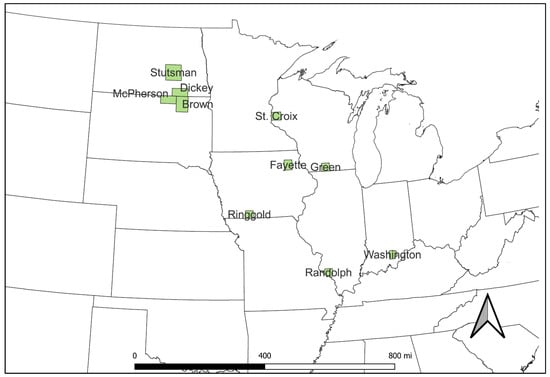
Figure 1.
Locations of study counties.
2. Materials and Methods
2.1. Land Use Identification
This study assessed land use for the period from 1985 to 2021 using three separate methods (Figure 2). Aerial imagery from the 1980s and 2000s was visually inspected for land use. Normalized Difference Vegetation Indices (NDVIs) developed from monthly composites of Landsat satellite imagery for the month of June were analyzed for land use. These images display higher values in June where natural vegetation is growing as crops have not emerged yet. Finally, NDVI values developed using the LandTrendr [18] algorithm on Landsat composites for spring, summer, and autumn were analyzed for the parcels. The LandTrendr algorithm was used to develop temporal curves which, when displayed in Google Earth Engine, displayed an averaged NDVI value for each parcel in spring, summer, and autumn for each year from 1985 to 2021. Parcels in crop will typically show a distinctive three-point curve with low spring and autumn values and high summer values. Crop-free fields typically have higher values in the spring and autumn from existing perennial vegetation but lower summer values. After a parcel was assessed using all three methods, a decision was made as to whether the parcel was in crop or in natural vegetation for each year. Figure 2 demonstrates the much higher peaks of the annual, temporal curves for crop and the more subdued curves for natural vegetation.
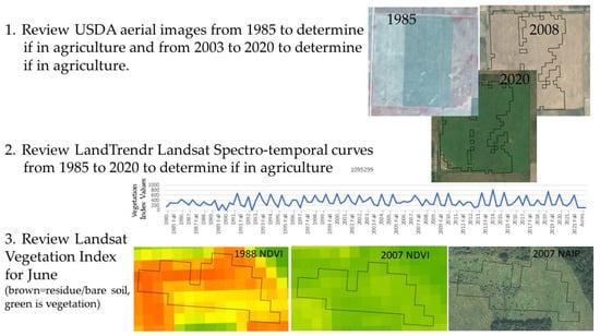
Figure 2.
Three methods for estimating land use from 1985 to 2020 for 100 points in each county.
In six states (responsible for 47% of corn planted in the United States in 2022 [13]: Iowa, Illinois, Indiana, North Dakota, South Dakota, and Wisconsin), a total of ten counties (one or two per state) were selected for analysis. Parcels that were previously identified by Lark et al. in a recent paper as grassland-to-cropland changes between 2008 and 2016 were considered [19]. The areas identified by Lark et al. overlap with areas previously identified by another research group for land use change [11]. In the present work, the 100 largest parcels in ten counties identified in the Lark paper for land use change were accessed and analyzed for land use change between a longer time horizon (1985 to 2021) using three different remote-sensing-based methods.
In the first method, USGS and USDA aerial imagery was reviewed for land use (Figure 3). There are several features in aerial imagery that indicate cropland or natural vegetation. Crops will grow uniformly throughout a parcel, while natural vegetation may have different patterns in the parcel and grow in clumps based on the amount and type of plants growing. Crops often have linear features indicative of rows. Natural vegetation may have little circles indicating shrubs or trees. Crops will be green in visible light photography and red in near-infrared photography, while natural vegetation may appear grey or brown in visible light and pink or grey in near-infrared. Also, occasionally, hay fields will have bales of hay somewhere in or near the field.
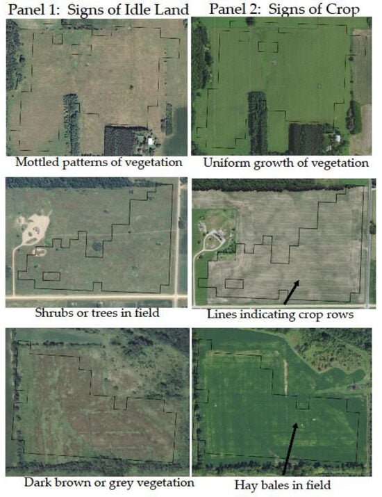
Figure 3.
Examples of methods used to delineate crop and idle parcels using USDA NAIP imagery. Arrows indicate location of lines indicating crop rows and locations of hay bales.
Imagery from two different government imagery programs was used: the USGS National High-Altitude Photography (NHAP) [20] and the USDA National Agriculture Imagery Program (NAIP) [21]. The NHAP program collected aerial photography from 1980 to 1989. Some of the imagery was black and white, while other imagery was color infrared (a combination of near-infrared and visible bands). The imagery was digitized and is available from the United States Geological Survey (USGS) EarthExplorer website with spatial resolutions from 1 to 4 m. The imagery is not georeferenced. The project used corner coordinates to create an approximate georeferencing to assist with finding parcels. One-meter imagery was available from 1983 to 1985 (depending on state) for all parcels.
The NAIP program offers aerial imagery collected in agricultural states on an annual or biennial basis (Figure 4). The spatial resolution of the imagery ranges from 1 to 2 m, and is either visible bands (red, green, and blue bands) or visible and near-infrared (red, green, blue, and near-infrared bands). For this study, a visual assessment of NAIP from 2003 to 2020 (depending on availability for each state) was used to identify potential land use.
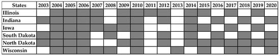
Figure 4.
Years with NAIP imagery for each state from 2003 to 2020 (in grey).
A series of Landsat satellites, including Landsat 1 (1972), Landsat 2 (1975), Landsat 3 (1978), Landsat 4 (1982), Landsat 5 (1984), Landsat 6 (1993), Landsat 7 (1999), Landsat 8 (2013), and Landsat 9 (2021), have been launched into orbit. Beginning with Landsat 4 in 1982, the Thematic Mapper instrument was included [22]. The Thematic Mapper offers continuous 30 m imagery in several bands in the visible and near-infrared range. The satellites only scan the same location on the earth’s surface once every 17 days and are impacted by cloud cover, sometimes limiting coverage. For the second method in this study, NDVI images were developed using Landsat 5, 7, and 8 using composite images for June of each year from 1985 to 2021 in Google Earth Engine. The imagery was corrected to surface reflectance removing atmospheric effects and a brown-to-green color scale was applied. Parcels with orange or yellow NDVI values (lower values) in June were crop (bare soil or residue) in June while parcels with green values (higher values) are likely natural vegetation as the vegetation is in the field all year and will start to grow with the warm weather in June (Figure 5).
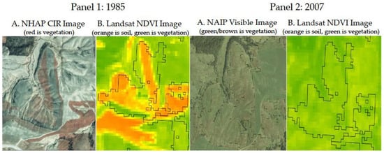
Figure 5.
Examples of land in crop and land in vegetation in aerial images and June Landsat NDVI.
For the third step, spectro-temporal curves were analyzed for each year using the LandTrendr algorithm. The LandTrendr algorithm is a time-series analysis technique for remote sensing and land cover change studies. It was developed to automatically detect and quantify changes in satellite imagery over time. By processing multiple temporal images, LandTrendr identifies changes in land cover. The algorithm is based on pixel-level spectral trajectories and can effectively distinguish between long-term land cover trends and short-term disturbances. For this study, spectro-temporal curves were created using LandTrendr in Google Earth Engine for each year from 1985 to 2021 for composite Landsat images in the spring (April–May), summer (mid-July to mid-August), and autumn (mid-October to mid-November). Graphs of these curves were plotted alongside the imagery of each parcel to assist in the land use assessment. Parcels with the lowest values in spring and autumn and highest numbers in summer in a particular year are crop with bare soil in the spring, vibrant vegetation in the summer, and low values after harvest. Parcels with the highest values in spring and fall and lowest values in summer are likely natural vegetation as the parcel are not uniformly planted and do not receive fertilizer and other elements that improve growth in the summer and are growing on the parcel in the spring and autumn (Figure 6). The parcel in Figure 6 has low spring/autumn to high summer LandTrendr values from 1985 to 2000, more subdued curves from 2001 to 2008, and more low spring/autumn LandTrendr values with high summer values from 2009 to 2021. This, combined with the aerial imagery and spring NDVI values for this parcel, led to the parcel being identified as an active crop field from 1985 to 2000, fallow or CRP from 2001 to 2008, followed by a return to crop in 2009.
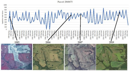
Figure 6.
Example of LandTrendr annual spectro-temporal curves for a parcel that transitioned between idle and crop.
2.2. Drivers of Land Use Change
To better understand the drivers for land use change, a list of landowners for parcels identified as change was sent to each respective state corn-grower association involved in the study. The grower associations identified farmers who were members that would be willing to provide an interview and were a good representation of farmers in the area and provided contact information. Detailed interviews were conducted with these growers. In total, nineteen farmers from four states (Stutsman and Dickey counties in North Dakota, Brown County in South Dakota, Fayette County in Iowa, and Washington County, Indiana) were interviewed regarding their land use decisions. Interviewing methods included telephone conversations, video meetings, and a Google Forms questionnaire (Appendix A). This is a small sample size, but it can be difficult to get farmers to discuss their on-farm practices. The Google Forms questionnaire was developed with the cooperation of the state grower associations. The grower associations provided many good questions which were focused specifically on the growers in their state. They also identified privacy concerns for the farmers and requested answers given or data provided by a single farmer not be included in this paper to protect this privacy. Each farmer had one to two parcels identified as conversion constituting close to 400 hectares associated with potential change to crop. The study used telephone and video meetings to follow up and ask more detailed questions after the Google Form was filled out by the farmer. These could last anywhere from 15 min to over an hour depending on the extent of the parcels identified as change, the willingness of the grower to speak, and other answers provided in the Google Forms questionnaire.
2.3. Carbon Change Assessment
The study analyzed SOC change from the parcels’ transitions between crop and non-crop using the System Approach to Land Use Sustainability (SALUS) model developed at Michigan State University. SALUS models crop, nutrient, soil, and water conditions at a daily time step using different management techniques. SALUS was parameterized to assess CRP type vegetation species for the non-crop years rotating with reduced-till corn for the crop years [22,23,24]. Reduced-till corn for the crop year was based on a separate survey by the USDA which showed a trend that most crop acres have been in some form of reduced tillage system, with 65% of all corn acres farmed under this practice [25,26].
The findings were then compared to the model results from the surrogate soil organic carbon model (SSOC) database that is part of the Carbon Calculator for Land Use and Land Management Change from Biofuel Production (CCLUB) developed by Argonne National Laboratory, which is integrated with the Greenhouse Gas Regulated Emissions in Technologies (GREET) model for greenhouse gas life cycle emissions modeling of biofuel pathways [5]. The SSOC model is originally based on Century, and it models SOC changes from land use change on a county-by-county basis for two different soil depths (30 cm and 100 cm) while averaging values for the two dominant soil textures in each county [27,28]. SSOC and SALUS are both process-based models that take weather, plant biomass, and soil textures into consideration among other variables [29]. SSOC aggregates the resulting carbon assessment by biomass feedstock and management practice to the county level, taking the two dominant soil textures of each county into consideration. SALUS is also a process-based model that measures outcomes down to the sub-field level [30].
3. Results
3.1. Land Use Identification
One thousand parcels of land were analyzed for this study, with results shown in (Figure 7). It was found that between 1985 and 2021, 371 of the parcels (9583 hectares) were in continuous cropland, 611 parcels (15,451 hectares) were transitioned into non-cropland and back to cropland at some point in the 36-year period (1985 to 2021) (CRP, idle, fallow). No parcels transitioned out of and back into crop more than once. Eighteen parcels (1.8%) (888 hectares) in cropland in 2021 did not appear to be in cropland in 1985 and were labeled as grassland-to-crop conversions for SALUS and CCLUB. This contrasts with Lark et al. [8], who found grassland-to-cropland conversion for all 1000 parcels between 2008 to 2016.
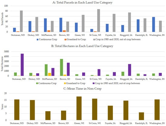
Figure 7.
Statistics for land use analysis. Subfigure (A) shows total parcels in each land use cate-gory, Subfigure (B) shows total hectares for each land use category, and Subfigure (C) shows the average number of years parcels were out of crop for counties.
For the parcels with transitions into non-cropland, the average non-crop phase across all parcels lasted 13.3 years. Using Brown County, SD as an example (Figure 8), 42 of the 100 parcels were in non-cropland for some period during 1985–2021. These periods were short (average 7.1 years), with only one parcel in non-cropland longer than in cropland during the full time period.
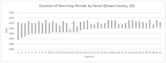
Figure 8.
Duration of non-crop periods by parcel in Brown County, South Dakota.
3.2. Farmer Surveys: Drivers of Land Use Change
The study returned nineteen grower surveys from four states (Stutsman and Dickey counties in North Dakota, Brown County in South Dakota, Fayette County in Iowa, and Washington County in Indiana). The surveys and interviews showed that of parcels in non-cropland, those in the Conservation Reserve Program (CRP) were the most likely to be returned to cropland. The most common reason provided for returning this land to active cropland was the difficulty in getting the land re-enrolled in the CRP (Figure 9). Other reasons given for returning land to cropland included low cattle prices when converting pasture and an improved return-on-investment analysis when looking at potential crop yields based on soil quality and increased rainfall patterns in the northwestern Corn Belt. South Dakota farmers cited a 2012 state tax law that taxes land above a given soil fertility calculated value as agriculture whether it is in crop or not. Those interviewees pointed towards a change in circumstances from their current practice rather than increased corn demand for their change in land use. These findings of drivers behind land use change are generally more consistent with Claasen et al. [31], who cite a broad range of often location-specific reasons for land transitions [31]. Importantly, more fields transitioned before 2008 (67%) than after 2008 (33%), indicating that 2008 was not likely a trigger point for additional land use conversion.
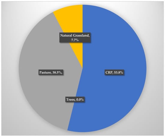
Figure 9.
Land conversions by surveyed farmers.
However, once changing circumstances confront farmers to return land to agriculture, they cited the use of the productivity index or soil fertility index in making decisions. Some marginal lands have been returned to the CRP or used for buffer strips in the field. The origins of land that was converted shows very little natural grassland. Many stated that they knew some of their land had to be left in grass or trees to reduce erosion and improve drainage. Farmers stated that if land is being returned to production, the parcels considered and chosen will be land previously in crop, as it is easier to clean up (remove rocks and stumps, etc.) than natural lands. Farmers also stated that the cost/return for land previously in agriculture is better known than for native grasslands and is therefore the choice for re-enrollment into agriculture.
3.3. Carbon Change Implications
The land use was used to parameterize SALUS for carbon stock assessment. SALUS shows mean positive delta soil organic carbon values across all counties and yearly model observations indicating increasing SOC (Table 1) with the larger mean carbon deltas observed for parcels which were “non-crop” for a period of years during the 36-year time period (1985 to 2021) than for “continuously in crop” (Table 2). Soil carbon deltas are sorted for all observed model values from largest losses to largest gains for crop and non-crop parcels and shown in Figure 10. The SOC values for “crop” in SALUS show larger soil carbon deltas, resulting both in larger SOC depletions and SOC gains than the “non-crop” SOC yearly observations.

Table 1.
Soil carbon results for different models.
Table 2.
Soil carbon results by crop vs. non-crop land use.
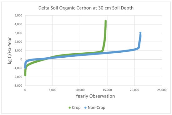
Figure 10.
SALUS model soil carbon delta for crop and non-crop parcels.
However, the delta soil organic values are increasing year over year as shown in Figure 11 for Brown County ND as an example county. This finding is consistent across all assessed counties (as indicated by the trendline equation shown for each county in Figure 11. This means that, in the aggregate, the studied parcels, despite their transitionary land use, will not observe soil carbon losses under our modeled assumptions.
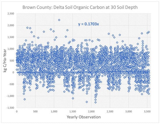
Figure 11.
Soil carbon deltas for Brown County.
The 30 cm SALUS SOC values are compared to the cropland-pasture values transitioning to reduced-till corn at 30 cm soil depth for the respective counties in CCLUB [5] (Figure 1). Despite methodological differences and different forms of spatial aggregation, both models produce similar results when simulating transitionary crop and non-crop areas. Specifically, both models produce mean positive soil carbon deltas at the county-level resolution.
4. Discussion
4.1. Land Use Identification
Across 1000 analyzed parcels and close to 36,000 yearly observations, the analysis showed that 371 parcels remained continuously in cropland, while 611 parcels did go into “non-crop” (CRP, idle, pasture, or fallow) for a few years from 1985 to 2021. This would make the latter category a subset of a defined land category in computable general equilibrium models termed the cropland–pasture category. This category is often accessed in these models when land conversions in response to price signals are expected. Only 18 parcels (1.8%) appeared to come from land not in crop in 1985 and constitute grassland-to-crop conversions.
All these parcels were delineated as change from natural grassland to crop in the Lark et al. analysis. Lark primarily used the USDA Cropland Data Layer (CDL) to develop the dataset used. Other studies such as Wright and Wimberly [11] and the World Wildlife Fund’s Plowprint Report [12] also used the CDL as a primary data source. While part of the issue with the satellite-based CDL is its accuracy for non-agricultural classes, this study has shown that the choice of the time horizon is also significant. Each of the above studies began their analysis in or close to the year when agricultural demand increased and did not consider lands previously in crop that were available for crop production with reduced SOC implications.
4.2. Drivers of Land Use Change
The underlying drivers for land use change were explored with 19 detailed farmer interviews across the studied counties. The study found that the land to be returned to crop was agricultural land in the Conservation Reserve Program (CRP) followed by pastureland. Reduced cattle prices and changing tax structures (taxing land above a soil quality value as agriculture whether it is in crop or not) and difficulty getting the land re-enrolled in the CRP were key drivers for converting pasture [31,32]. The interviewees pointed towards a change in return from their current practice rather than increased corn demand for their change in land use.
Based on the surveys, farmers take much more into consideration than current demand when determining land use for a given year. Other land uses such as cattle production or conservation, long-term return on investment, and weather play important roles. Also important is that farmers are more likely to use land previously in agriculture when increasing agricultural land. These parcels are typically more productive and easier to convert to crops.
4.3. Carbon Change Assessment
The SOC changes were estimated using both the SALUS and the GREET-CCLUB model. SALUS was specifically parameterized using the crop and non-crop time intervals for each parcel. Both models returned consistent results when parameterized with cropland–pasture type vegetation species rotating in and out of reduced-till corn-on-corn rotations, with both carbon models returning, on average, positive soil carbon deltas. In SALUS, the soil carbon deltas are larger for parcels alternating between “crop” and “non-crop” rotations when compared to parcels that are consistently in “crop”. However, lands consistently in “crop” also exhibit mean average positive soil carbon values.
Previous research on the same parcels that the present paper studied focused on a narrow time window (e.g., 2008–2016) and labeled land use change within that time frame as grassland-to-cropland conversions and postulated biofuel production to be the driver of land conversion. The present work, however, finds that 98.2 percent of the same parcels referenced in the literature were in agriculture in 1985 and toggled between crop and non-crop uses based on a variety of drivers. Importantly, the study finds that lands transitioning to agricultural lands from pastureland, idle, fallow, and unused state were agricultural lands in the past and not native grasslands. This is corroborated with farmer interviews who mentioned that land-clearing costs are much lower for previous agricultural lands than for native grasslands.
5. Conclusions
The analysis presented in this paper aims to increase the understanding of transitional land that changes between crop and non-crop uses with respect to the underlying patterns, drivers, and carbon implications. Methodologically, the analysis is based on (a) identifying the land use patterns of 1000 parcels from 1985 to 2021 with a combination of several remote-sensing tools including USDA NAIP imagery analysis combined with satellite-based geospatial evaluations, followed by (b) in-depth grower interviews to understand the drivers for land use change, and (c) an assessment of the carbon implications resulting from the identified land use patterns.
Across 1000 analyzed parcels and close to 36,000 yearly observations, the analysis showed that 371 parcels remained continuously in cropland, while 611 parcels did go into “non-crop” (CRP, idle, pasture, fallow) for a few years from 1985 to 2021. This would make the latter category a subset of a defined land category in computable general equilibrium models termed the cropland–pasture category. This category is often accessed in these models when land conversions in response to price signals are expected. Only 18 parcels (1.8%) appeared to come from land not in crop in 1985 and constitute grassland-to-crop conversions.
The underlying drivers for land use change were explored with 19 detailed grower interviews across the studied counties. The study found that the most likely land to be returned to crop was agricultural land in the Conservation Reserve Program (CRP) followed by pastureland. Reduced cattle prices and changing tax structures (taxing land above a soil quality value as agriculture whether it is in crop or not) and difficulty getting the land re-enrolled in the CRP were key drivers for converting pasture. Interestingly, the interviewees pointed towards a change in return from their current practice rather than increased corn demand for their change in land use.
The carbon implications were assessed using both the SALUS and the GREET-CCLUB model. SALUS was specifically parameterized using the crop and non-crop time intervals for each parcel. Both models returned consistent results when parameterized with cropland–pasture type vegetation species rotating in and out of reduced-till corn-on-corn rotations, with both carbon models returning, on average, positive soil carbon deltas. In SALUS, the soil carbon deltas are larger for parcels alternating between “crop” and “non-crop” rotations when compared to parcels that are consistently in “crop”. However, lands consistently in “crop” also exhibit mean average positive soil carbon values.
Previous research on the same parcels that the present paper studied focused on a narrow time window (e.g., 2008–2016) and labeled land use change within that time frame as grassland-to-cropland conversions and postulated biofuel production to be the driver of land conversion. The present work, however, finds that 98.2 percent of the same parcels referenced in the literature were in agriculture in 1985 and toggled between crop and non-crop uses based on a variety of drivers. Importantly, the study finds that lands transitioning to agricultural lands from pastureland, idle, fallow, and unused state were generally agricultural lands in the past and not native grasslands. This is directly corroborated with grower interviews who mentioned that land-clearing costs are much lower for previous agricultural lands than for native grasslands.
Furthermore, when two prominent process-based soil carbon models were parameterized with the parcels’ specific geography and a transition between corn (reduced till) and CRP vegetation species, both models returned increasing soil carbon values across all parcels. In conclusion, the present work points to the need to conduct any land use change analysis over much longer periods of time than is often practiced to fully incorporate a parcel’s land use history. Secondly, land that is returned out of the CRP, fallow, idle, or temporary pasture state into a corn cropping pattern (reduced till) will still show, on average, increasing soil carbon levels over time. A key practical significance of this research is that the increase in soil carbon over a longer time horizon for transitional land can now properly be reflected in carbon accounting models that access these transitional lands for additional bioenergy and biofuel feedstock production. Finally, agricultural organizations working with growers should ensure that conservation management practices are continuously encouraged as these practices ensure that the carbon deltas after any land conversion remain continuously positive.
The limitations of this study include the potential for error by the classifier when conducting visual assessments of year-over-year land use and overlap between the spectral response of crops, especially hay, and idle cropland. Future research in this area should include carbon implications from a comprehensive suite of climate smart agricultural practices (cover crops, no-till, and manure application) and include additional parcels in the western Corn Belt where land use drivers may differ.
Author Contributions
Conceptualization, S.M.; Methodology, K.C.; Formal analysis, S.M.; Investigation, S.M.; Writing—original draft, K.C.; Writing—review & editing, S.M.; Supervision, S.M.; Project administration, S.M.; Funding acquisition, S.M. All authors have read and agreed to the published version of the manuscript.
Funding
This research was funded by the Illinois Corn Marketing Board, Iowa Corn Growers Association, Wisconsin Corn Promotion Board, South Dakota Corn Utilization Council, Indiana Soybean Alliance/Indiana Corn Marketing Council, North Dakota Corn Council.
Data Availability Statement
All data except for individual farmer interviews will be made available upon request.
Acknowledgments
The authors express their gratitude to Bruno Basso and Lydia Price at Michigan State University for their support on the SALUS model simulations results.
Conflicts of Interest
Author Kenneth Copenhaver was employed by the company CropGrower LLC. The remaining author declares that the research was conducted in the absence of any commercial or financial relationships that could be construed as a potential conflict of interest.
Appendix A
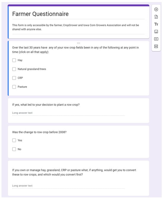
Figure A1.
Template for Farmer Questionnaire.
References
- Tyner, W.; Taheripour, F. Biofuels, policy options, and their implications: Analyses using partial and general equilibrium approaches. J. Agric. Food Ind. Organ. 2008, 6, 2. [Google Scholar] [CrossRef]
- Taheripour, F.; Mueller, S.; Kwon, H.; Khanna, M.; Emery, I.; Copenhaver, K.; Wang, M. Comments on “Environmental Outcomes of the US Renewable Fuel Standard”. 2021. Available online: https://greet.es.anl.gov/files/comment_environ_outcomes_us_rfs (accessed on 14 December 2023).
- Emery, I.; Mueller, S.; Qin, Z.; Dunn, J. Evaluating the Potential of Marginal Land for Cellulosic Feedstock Production and Carbon Sequestration in the United States. Environ. Sci. Technol. 2017, 51, 733–741. [Google Scholar] [CrossRef] [PubMed]
- Plevin, R.; Gibbs, H.; Duffy, J.; Yui, S.; Yeh, S. Agro-Ecological Zone Emission Factor (AEZ-EF) Model 2014. No. 1236-2019-175. Volume 47. Available online: https://ageconsearch.umn.edu/record/283433/ (accessed on 14 December 2023).
- Kwon, H.; Liu, X. FD-CIC and CCLUB for Biofuel Feedstocks. GREET Training Workshop 2022. Available online: https://greet.anl.gov/publication-workshop_2022_fdcic_cclubde (accessed on 14 December 2023).
- 6. IIASA-FOLU Integrated Scenarios. Global Biosphere Management Model Project. Available online: https://iiasa.ac.at/models-tools-data/globiom (accessed on 15 December 2023).
- IPCC. Climate Change and Land, an IPCC Special Report on Climate Change, Desertification, Land Degradation, Sustainable Land Management, Food Security, and Greenhouse Gas Fluxes in Terrestrial Ecosystems; Chapter 2 of IPCC 2019 Climate Change and Land; IPCC: Geneva, Switzerland, 2019. [Google Scholar]
- Lark, T.J.; Salmon, J.M.; Gibbs, H.K. Cropland expansion outpaces agricultural and biofuel policies in the United States. Environ. Res. Lett. 2015, 10, 044003. [Google Scholar] [CrossRef]
- Lark, T.; Mueller, R.; Johnson, J.; Gibbs, H. Measuring land-use and land-cover change using the U.S. department of agriculture’s cropland data layer: Cautions and recommendations. Int. J. Appl. Earth Obs. Geoinf. 2019, 62, 224–235. [Google Scholar] [CrossRef]
- Copenhaver, K.; Hamada, Y.; Mueller, S.; Dunn, J.B. Examining the Characteristics of the Cropland Data Layer in the Context of Estimating Land Cover Change. ISPRS Int. J. Geo-Inf. 2021, 10, 281. [Google Scholar] [CrossRef]
- Wright, K.; Wimberly, M. Recent land use change in the Western Corn Belt threatens grasslands and wetlands. Proc. Natl. Acad. Sci. USA 2013, 110, 4134–4139. [Google Scholar] [CrossRef] [PubMed]
- World Wildlife Foundation Annual Plowprint Report. Available online: https://www.worldwildlife.org/projects/plowprint-report (accessed on 15 December 2023).
- USDA National Agricultural Statistics Service Quick Stats. Survey Data. 2023. Available online: https://quickstats.nass.usda.gov/ (accessed on 15 December 2023).
- Tan, M.; Li, Y. Spatial and Temporal Variation of Cropland at the Global Level from 1992 to 2015. J. Resour. Ecol. 2019, 10, 235–245. [Google Scholar]
- Auch, R.F.; Wellington, D.F.; Taylor, J.L.; Stehman, S.V.; Tollerud, H.J.; Brown, J.F.; Loveland, T.R.; Pengra, B.W.; Horton, J.A.; Zhu, Z.; et al. Conterminous United States Land-Cover Change (1985–2016): New Insights from Annual Time Series. Land 2022, 11, 298. [Google Scholar] [CrossRef]
- Johnson, D.; Mueller, R.; Willis, P. The utility of the Cropland Data Layer for monitoring US grassland extent. In Proceedings of the 3rd Biennial Conference on the Conservation of America’s Grasslands, Fort Collins, CO, USA, 29 September–1 October 2015; National Wildlife Federation: Washington, DC, USA, 2015; pp. 15–19. [Google Scholar]
- Reitsma, K.; Clay, D.; Clay, S.; Dunn, J.; Reese, C. Does the U.S. Cropland Data Layer Provide an Accurate Benchmark for Land-Use Change Estimates? Agron. J. 2015, 108, 226. [Google Scholar] [CrossRef]
- LandTrendr Home Page, Kennedy Geospatial Lab, University of Oregon. Available online: https://geotrendr.ceoas.oregonstate.edu/landtrendr/ (accessed on 16 December 2023).
- Lark, T.; Schelly, I.; Gibbs, H. Accuracy, Bias, and Improvements in Mapping Crops and Cropland across the United States Using the USDA Cropland Data Layer. Remote Sens. 2021, 13, 968. [Google Scholar] [CrossRef]
- USGS National High Altitude Photography Program. 2023. Available online: https://www.usgs.gov/centers/eros/science/usgs-eros-archive-aerial-photography-national-high-altitude-photography-nhap (accessed on 16 December 2023).
- USDA National Aerial Imagery Program. 2023. Farm Services Agency. Available online: https://www.fsa.usda.gov/programs-and-services/aerial-photography/imagery-programs/naip-imagery/ (accessed on 16 December 2023).
- Hemati, M.; Hasanlou, M.; Mahdianpari, M.; Mohammadimanesh, F. A Systematic Review of Landsat Data for Change Detection Applications: 50 Years of Monitoring the Earth. Remote Sens. 2021, 13, 2869. [Google Scholar] [CrossRef]
- Martinez-Feria, R.; Basso, B. Predicting soil carbon changes in switchgrass grown on marginal lands under climate change and adaptation strategies. GCB Bioenergy 2020, 12, 742–755. [Google Scholar] [CrossRef]
- Basso, B.; Ritchie, J.T.; Grace, P.R.; Sartori, L. Simulation of Tillage Systems Impact on Soil Biophysical Properties Using the SALUS Model; Ital. J. Agron. Riv. Agron. 2006, 4, 677–688. [Google Scholar]
- Basso, B.; Ritchie, J. Simulating crop growth and biogeochemical fluxes in response to land management using the SALUS model. In The Ecology of Agricultural Landscapes: Long-Term Research on the Path to Sustainability; Hamilton, S.K., Doll, J.E., Robertson, G.P., Eds.; Oxford University Press: New York, NY, USA, 2015; pp. 252–274. [Google Scholar]
- Claassen, R.; Bowman, M.; McFadden, J.; Smith, D.; Wallander, S. Tillage Intensity and Conservation Cropping in the United States; EIB-197; U.S. Department of Agriculture, Economic Research Service: Washington, DC, USA, 2018. [Google Scholar]
- Qin, Z.; Dunn, J.; Kwon, H.; Mueller, S.; Wander, M. Soil carbon sequestration and land use change associated with biofuel production: Empirical evidence. GCB Bioenergy 2016, 8, 66–80. [Google Scholar] [CrossRef]
- Xu, H.; Sieverding, H.; Kwon, H.; Clay, D.; Stewart, C.; Johnson, J.; Qin, Z.; Karlen, D.; Wang, M. A global meta-analysis of soil organic carbon response to corn stover removal. GCB-Bioenergy 2019, 11, 1215–1233. [Google Scholar] [CrossRef]
- Mandal, A.; Majumder, A.; Dhaliwal, S.; Toor, A.; Kumar Mani, P.; Naresh, R.; Gupta, R.; Mitran, T. Impact of agricultural management practices on soil carbon sequestration and its monitoring through simulation models and remote sensing techniques: A review. Crit. Rev. Environ. Sci. Technol. 2022, 52, 1–49. [Google Scholar] [CrossRef]
- Basso, B. Crop Modeling Can Scale Regenerative Agriculture to Address Climate Change. 9 March 2022. Available online: https://www.greenbiz.com/article/crop-modeling-can-scale-regenerative-agriculture-address-climate-change#:~:text=SALUS%20is%20a%20validated%20process,computer%2C%20like%20a%20digital%20twin (accessed on 17 December 2023).
- Classen, R.; Carriazo, F.; Cooper, J.; Hellerstein, D.; Udea, K. Grassland to Cropland Conversion in the Northern Plains: The Role of Crop Insurance, Commodity, and Disaster Programs; ERR-120; U.S. Department of Agriculture, Economic Research Service: Washington, DC, USA, 2011. [Google Scholar]
- Hellerstein, D. The US Conservation Reserve Program: The evolution of an enrollment mechanism. Land Use Policy 2017, 63, 601–610. [Google Scholar] [CrossRef]
Disclaimer/Publisher’s Note: The statements, opinions and data contained in all publications are solely those of the individual author(s) and contributor(s) and not of MDPI and/or the editor(s). MDPI and/or the editor(s) disclaim responsibility for any injury to people or property resulting from any ideas, methods, instructions or products referred to in the content. |
© 2024 by the authors. Licensee MDPI, Basel, Switzerland. This article is an open access article distributed under the terms and conditions of the Creative Commons Attribution (CC BY) license (https://creativecommons.org/licenses/by/4.0/).