Dynamic Evaluation of Water Resources Management Performance in the Yangtze River Economic Belt

Abstract

The evaluation of water resources management performance (WRMP) can provide guidance for water resources management. This paper constructs a scientific WRMP evaluation index system based on “water resources–water environment–water ecology”. Secondly, the game variable weight matter–element extension model is appropriately introduced to dynamically evaluate the WRMP level of the provinces (cities) in the YREB from 2012 to 2021, and Arcgis is used to analyze the spatial and temporal variations in the performance level of each sub-system. Lastly, a geographical detector model is used to explore the main factors influencing the WRMP in the Yangtze River Economic Balt (YREB). The main findings are as follows: (1) The overall provincial WRMP level in the YREB has been improving from 2012 to 2021, and the performance of water resource utilization (WRU) and water environment treatment (WET) are high in the east and low in the west, while the performance of water ecological protection (WEP) shows a trend of continuous improvement. (2) Compared with the model without variable weight modification, the game variable weight matter–element extension model can reflect the influence of the measured value of the index on the evaluation result as much as possible. (3) The top eight factors that have a greater impact on the WRMP level are the industrial water conservation rate, water resource development and utilization rate, water resource sustainability index, sewage diameter ratio, urban water penetration rate, industrial wastewater treatment completion rate, ecological construction and protection of the year to complete the investment in GDP, and the water ecological carrying capacity growth rate. The interaction types of each influence factor are nonlinear enhancement and two-factor enhancement.

1. Introduction

Water resources are essential for human survival and development [1], and they play a supportive role in socio-economic and ecological sustainable development [2]. The insufficient reserves of freshwater resources in the world and the improper handling of water resources have caused a severe scarcity of freshwater resources that are accessible to humanity given the current circumstances [3]. The most recent edition of the United Nations World Water Development Report reveals that approximately 26% of the global population lacks access to safe drinking water, 3.6 billion individuals lack properly managed sanitation facilities, and 2 to 3 billion people are facing a water scarcity predicament. In an effort to address this predicament, numerous nations have started to focus on water resource management, set up a contemporary water resources management system to fulfill the demands of sustainable development, and persist in investigating the assessment and oversight mechanism of WRMP tailored to their respective national circumstances to tackle the water resource crisis.

China is a large developing country with a serious shortage of water resources, with per capita water resources accounting for only one-quarter of the world average [4]. Water resources are not being used efficiently, the effective utilization coefficient of farmland irrigation water is low, industrial water consumption is 2–3 times greater than the global level, and the leakage rate of the urban water supply network is as high as 20% [5]. Furthermore, the rapid socio-economic development, the increased demand for clean water resources among residents, the gradual increase in industrial and domestic sewage discharge, and the persistent destruction of the water ecological environment have led to the aggravation of China’s water scarcity crisis [6,7]. In order to ameliorate this circumstance, China has released a range of policy documents, including the Action Plan for the Prevention and Control of Water Pollution, the 14th Five-Year Plan for Ecological Environmental Protection and Supervision, and the Implementation Plan for Industrial Wastewater Recycling, and they have carried out the fine management of water resources to reduce the consumption of water resources, improve the water environment, and repair the water ecology. Despite the fact that these policies protect the water ecology by controlling the total amount of water consumption and improving the quality of water resources, the specific situation of their management level and the influencing factors are difficult to clarify in time. Consequently, in order to effectively monitor the level of water resources management, it is particularly important to examine the WRMP from various aspects and seek its main influencing factors.

The YREB is one of the regions with the origin, development, and prosperity of Chinese civilization. Its high-quality development is related to the major strategy of China’s national development [8,9]. In recent years, the problems of water resource shortage and water ecology damage in the YREB have become increasingly prominent [10]. In 2017, the state issued the YREB Ecological Environmental Protection Plan, which, for the first time, put forward the goal of protecting the YREB on a large scale. In 2019, the Ministry of Ecology and Environment and the Development and Reform Commission jointly issued the Yangtze River Protection and Restoration Battle Action Plan, which explicitly proposed to solve the outstanding ecological and environmental problems in the Yangtze River, and it clearly put forward the requirements for the “three waters” coordination of the WRU, WET, and WEP in the Yangtze River. The overall planning of “three waters” is a new type of water resources management system in the new era. The WRU is the foundation, the WET is the breakthrough, and the WEP is the goal. The realization of any “one water” requires the coordinated promotion of the other “two waters” [11]. In addition, in order to accurately grasp the WRMP and timely adjust water resources management measures and strategies, the Ministry of Water Resources of China also conducted a thorough review of water resources management and established a complete WRMP evaluation system. Accordingly, in order to improve the current situation of water resources management, it is of great significance to reasonably construct a WRMP evaluation system, evaluate its management level, and explore its main influencing factors.

Water resources management involves administration authorities managing the development, utilization, scheduling, and protection of water resources through economic, technical, and legal methods. The socioeconomic and ecological growth of the area are greatly impacted by these governmental measures. To the best of our knowledge, the current research on water resources management primarily concentrates on the following areas: the development and preservation of water resources, the optimal allocation of water resources, and the carrying capacity of water resources [12,13,14] Most of these studies were focused on the behavior of water resources management. There were also some studies that started from the results of water resources management [15], and they used different methods to evaluate different areas from different perspectives. Specifically, first of all, in terms of evaluation methods, most of the studies chose a principal component analysis [16], the method of approximating the ideal solution ranking (TOPSIS) [17], multiple regression [18],particle swarm optimization algorithms [19], object meta-analysis [20], and other methods for the evaluation of the WRMP, but these methods ignored the complexity of the water resources management evaluation system and the impact of the fluctuation in the actual value of each specific evaluation index on the evaluation results. In contrast, the game variable weight material–element topological model introduces variable weight modification on the basis of the traditional material element topological model, which can dynamically reflect the actual change in the data according to their actual value, and then make the evaluation results closer to the actual situation [21]. Secondly, in terms of evaluation perspectives, some scholars evaluated the WRMP from the three perspectives of society, economy, and the environment [22,23], and some scholars explored the WRMP from the perspective of the “three red lines” or other perspectives [20,24]. Finally, as far as research areas are concerned, some scholars have used arid zones [22], watersheds [23], irrigated areas [25,26] and lakes [27] as research areas, and have also used the national water sector [28] as a research object for WRMP assessment. In summary, it can be seen that the research on WRMP still needs to be further improved.

Although the WRMP has been extensively studied, the following deficiencies remain: (1) The WRMP is different at different scales, but the existing literature mostly focused on small scales such as irrigation areas and lake water, and pays insufficient attention to the WRMP in large-scale regional units such as economic belts. (2) The existing research is biased in the selection of evaluation methods, and it failed to modify the comprehensive weight according to the actual value of the data, which affected the accuracy of the evaluation results. Therefore, based on the analysis framework of the WRMP of “water resources–water environment–water ecology”, this paper uses 11 provinces (cities) in the YREB as the research object to study the WRMP of large-scale regional units. Meanwhile, the improved game variable weight matter–element extension model is innovatively introduced into the WRMP evaluation level, and it is combined with the geographical detector model to analyze the spatial and temporal states of the WRMP and explore the main factors affecting the WRMP level.

The rest of the paper is organized as follows: The second part introduces the research field, methods, index system, and data sources. The third part expounds the main research results, the fourth part discusses the above results, and the fifth part puts forward the main conclusions and suggestions of this paper.

2. Materials and Methods

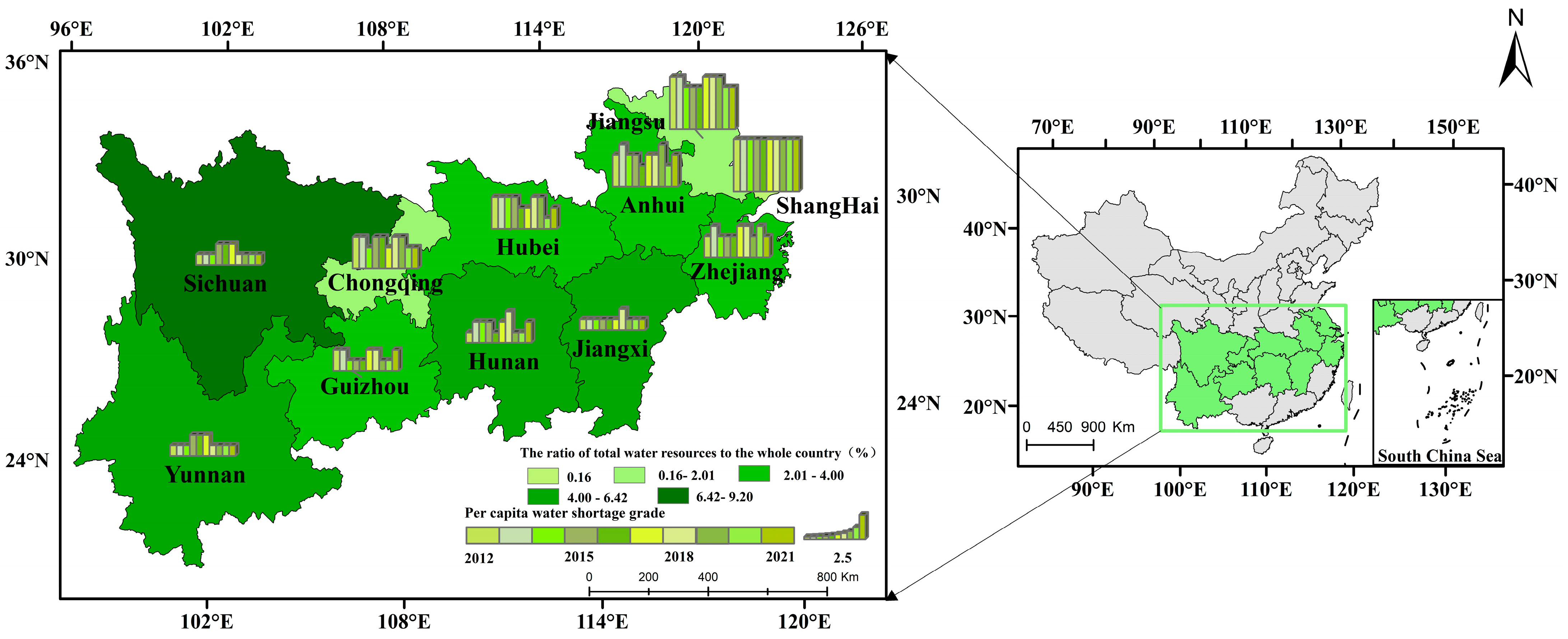
2.1. Study Area

The YREB is an inland economic belt with global influence; a coordinated development belt for interaction and cooperation in the eastern, central, and western regions of China; an inward and outward opening belt with comprehensive advancement along the coast and along the river and the border; as well as a pioneering demonstration belt for ecological civilization construction. It covers nine provinces and two cities, spanning three regions including Eastern China (Shanghai, Zhejiang, and Jiangsu), Central China (Anhui, Jiangxi, Hubei, and Hunan), and Western China (Sichuan, Chongqing, Yunnan, and Guizhou). The area is about 2052.3 square kilometers, accounting for 21.4% of the total area of the country, and the population and GDP comprise more than 40% of the country. The YREB has a good water resource endowment, and its total water resources account for about 44% of the total water resources in the country. However, due to its large population, its per capita water resources comprise lower than 25% of the world’s average. According to the 2012–2021 China Water Resources Bulletin and the Water Resources Statistics Bulletin of each province, the total water resources of the Sichuan, Hunan, Yunnan, and Jiangxi provinces account for a higher proportion of the whole country’s total water resources in the past ten years. Simultaneously, in terms of per capita water resources, the province’s per capita water resources in most years are in a state of mild and above (moderate, severe, and extreme) water shortage, while Shanghai has been in extreme water shortage (less than 500 m³) during the past decade (as shown in Figure 1). In addition, the rapid development of industrial and agricultural production and urban construction has led to frequent water environment pollution in the basin and prominent water ecological risks. However, under the guidance of policies such as the Action Plan for the Protection and Restoration of the Yangtze River, the Action Plan for the Prevention and Control of Water Pollution, and the Strictest Water Resources Management System, the YREB has preliminarily improved in water resources control and water ecological environment. It is still facing challenges in the conservation and intensive use of water resources and in the management and protection of the water ecological environment.

2.2. Research Methods

The matter–element extension evaluation model of this paper is based on the traditional matter–element extension evaluation model. Firstly, the game theory model is used to minimize the deviation between the subjective and objective weights. Secondly, combined with the variable weight theory, according to the actual value of each index, the determined comprehensive weight is dynamically modified to obtain the dynamic weight of each index. The flow chart of the comprehensive evaluation model is shown in Figure 2.

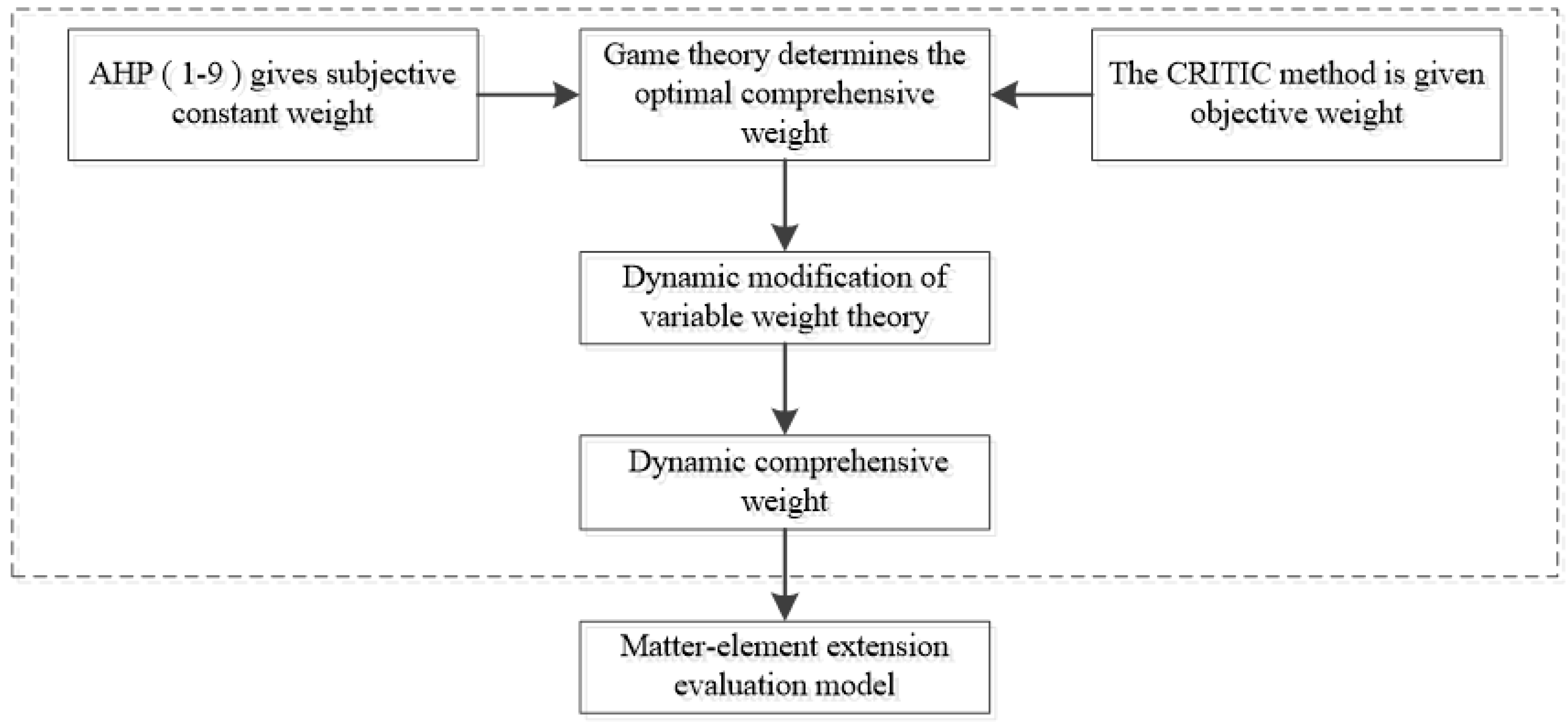
2.2.1. Determination of Index Weight

(1)

Determination of subjective weights

The Analytic Hierarchy Process (AHP) is used as a quantitative treatment of qualitative problems, and it has the characteristics of being systematic and organized. This method is now widely used in subjective evaluation, and the specific calculation steps are referenced in the literature [29,30,31,32].

(2)

Determination of objective weight based on CRITIC method

Compared to the entropy weighting method, the Criteria Importance Through Intercriteria Correlation (CRITIC) method takes into account both the variability and correlation between indicators, making the objective weighting more reasonable [33]. The specific calculation steps are as follows:

Step one: Suppose there are m evaluation indexes and n evaluation objects. The original matrix of WRMP evaluation is established as $X={\left({\mathrm{x}}_{\mathrm{i}\mathrm{j}}\right)}_{\mathrm{m}\times \mathrm{n}}$. Due to the differences in dimension and the order of magnitude between indicators, the indicator data should be standardized before using the CRITIC method to eliminate the problems of different quantitative indicators. The specific formulas are as follows:

If the evaluation index is a positive index, that is, the larger the value, the better, then positive normalization processing is used:

$${\mathrm{x}}_{\mathrm{i}\mathrm{j}}^{\prime }=\frac{{\mathrm{x}}_{\mathrm{i}\mathrm{j}}-{\mathrm{x}}_{\mathrm{i}\mathrm{m}\mathrm{i}\mathrm{n}}}{{\mathrm{x}}_{\mathrm{i}\mathrm{m}\mathrm{a}\mathrm{x}}-{\mathrm{x}}_{\mathrm{i}\mathrm{m}\mathrm{i}\mathrm{n}}}$$

(1)

If the evaluation index is a negative index, that is, the smaller the value, the better, then negative normalization is used:

$${\mathrm{x}}_{\mathrm{i}\mathrm{j}}^{\prime }=\frac{{{\mathrm{x}}_{\mathrm{i}\mathrm{m}\mathrm{a}\mathrm{x}}-\mathrm{x}}_{\mathrm{i}\mathrm{j}}}{{\mathrm{x}}_{\mathrm{i}\mathrm{m}\mathrm{a}\mathrm{x}}-{\mathrm{x}}_{\mathrm{i}\mathrm{m}\mathrm{i}\mathrm{n}}}$$

(2)

where ${\mathrm{x}}_{\mathrm{i}\mathrm{j}}^{\prime }$ is the standardized data; ${\mathrm{x}}_{\mathrm{i}\mathrm{j}}$ represents the original data of the ith evaluation index in the jth evaluation object; ${\mathrm{x}}_{\mathrm{i}\mathrm{m}\mathrm{a}\mathrm{x}}$ and ${\mathrm{x}}_{\mathrm{i}\mathrm{m}\mathrm{i}\mathrm{n}}$ represent the ith the maximum and minimum values of the evaluation indexes in the j evaluation objects; $\mathrm{i}=\mathrm{1,2},3\cdots m;\mathrm{a}\mathrm{n}\mathrm{d} \mathrm{j}=\mathrm{1,2},3\cdots n$.

Step two: The standard deviation ${\delta }_i$ is used to represent the contrast of the ith index.

$${\delta }_i=\sqrt{\frac{{\sum }_{j=1}^n{({\mathrm{x}}_{\mathrm{i}\mathrm{j}}^{\prime }-\overline{x_i^{\prime }})}^2}{n-1}}$$

(3)

$$\overline{x_i^{\prime }}=\frac{1}{n}{\sum }_{j=1}^n{\mathrm{x}}_{\mathrm{i}\mathrm{j}}^{\prime }$$

(4)

$\overline{x_i^{\prime }}$ is the average value of the ith index [34].

Step three: $f_i$ represents the conflict between the index $i$ and the other indexes.

$$f_i={\sum }_{g=1}^m(1-r_{gi})$$

(5)

where $r_{gi}$ is the correlation coefficient between index g and index i [35].

Step four: $Z_i$ represents the information carrying capacity of the calculated index $i$.

$$Z_i={\delta }_i·f_i$$

(6)

Step five: The objective weight of index $i$ is determined to be $W_i$.

$$W_i=\frac{Z_i}{{\sum }_{i=1}^m{Z}_i}$$

(7)

(3)

Game theory determines the comprehensive weight

The combination weighting method of game theory is based on the Nash equilibrium as the goal, coordinating the conflict between subjective and objective weights, and finding the consistency and compromise between weights. The process is an integration of mutual comparison and coordination, and it can realize the optimization of weights [21,36]. It includes the following five steps:

Step one: Assuming that there are k methods for weighting, there are k basic weight sets, $W_k=${$W_{k1},W_{k2},\dots W_{km}$}$(k=\mathrm{1,2},\dots L)$, where $m$ is the number of WRMP evaluation indicators, $k$ is the number of weight determination methods, and $k$is 2 in this paper. Let $\lambda$ = {${\mathsf{\lambda }}_1,{\mathsf{\lambda }}_{2,}\dots {\mathsf{\lambda }}_L$} be a linear combination coefficient; then, the combination weight is

$$W={\sum }_{\mathrm{k}=1}^{\mathrm{L}}{\mathsf{\lambda }}_{\mathrm{k}}{\mathrm{W}}_{\mathrm{k}}^{\mathrm{T}}({\mathsf{\lambda }}_{\mathrm{k}}>0,{\sum }_{\mathrm{k}=1}^{\mathrm{L}}{\mathsf{\lambda }}_{\mathrm{k}}=1,\mathrm{k}=\mathrm{1,2},\dots \mathrm{L})$$

(8)

Step two: According to the idea of game theory, the optimal ${\mathrm{W}}^{\mathrm{*}}$ is found in the possible vector set, and the linear combination coefficient is optimized to minimize the deviation of $\mathrm{W}$ and ${\mathrm{W}}_{\mathrm{k}}$.

$$\min {‖{\sum }_{\mathrm{k}=1}^{\mathrm{L}}{\mathsf{\lambda }}_{\mathrm{k}}{\mathrm{W}}_{\mathrm{k}}^{\mathrm{T}}-{\mathrm{W}}_{\mathrm{k}}‖}_2, (\mathrm{k}=\mathrm{1,2},\dots \mathrm{L})$$

(9)

${\mathrm{W}}_{\mathrm{k}}^{\mathrm{T}}$ is the transformation of the basic weight vector set; ${‖f\left(x\right)‖}_2=\sqrt{{\int }_a^b{f}^2\left(x\right)dx}$ represents the 2-norm numerical analysis [37].

Step three: According to the differential properties of the matrix, the linear differential equations of the first derivative condition of the above optimization are determined as follows:

$$\left[\begin{array}{cccc}{\mathrm{W}}_1{\mathrm{W}}_1^{\mathrm{T}}& {\mathrm{W}}_1{\mathrm{W}}_2^{\mathrm{T}}& \cdots & {\mathrm{W}}_1{\mathrm{W}}_{\mathrm{L}}^{\mathrm{T}}\\ {\mathrm{W}}_2{\mathrm{W}}_1^{\mathrm{T}}& {\mathrm{W}}_2{\mathrm{W}}_2^{\mathrm{T}}& \cdots & {\mathrm{W}}_2{\mathrm{W}}_{\mathrm{L}}^{\mathrm{T}}\\ ⋮& ⋮& ⋮& ⋮\\ {\mathrm{W}}_{\mathrm{L}}{\mathrm{W}}_1^{\mathrm{T}}& {\mathrm{W}}_{\mathrm{L}}{\mathrm{W}}_2^{\mathrm{T}}& \cdots & {\mathrm{W}}_{\mathrm{L}}{\mathrm{W}}_{\mathrm{L}}^{\mathrm{T}}\end{array}\right]\left[\begin{array}{c}{\mathsf{\lambda }}_1\\ {\mathsf{\lambda }}_2\\ \begin{array}{c}⋮\\ {\mathsf{\lambda }}_{\mathrm{L}}\end{array}\end{array}\right]=\left[\begin{array}{c}{\mathrm{W}}_1{\mathrm{W}}_1^{\mathrm{T}}\\ {\mathrm{W}}_2{\mathrm{W}}_2^{\mathrm{T}}\\ \begin{array}{c}⋮\\ {\mathrm{W}}_{\mathrm{L}}{\mathrm{W}}_{\mathrm{L}}^{\mathrm{T}}\end{array}\end{array}\right]$$

(10)

Step four: The combination coefficient ${\lambda }_k$ obtained above is normalized to obtain ${\lambda }_k^{*}$.

$${\lambda }_k^{*}=\frac{{\mathsf{\lambda }}_k}{{\sum }_{k=1}^L{\mathsf{\lambda }}_k}$$

(11)

Step five: The combined weight ${\mathrm{W}}^{\mathrm{*}}$ is obtained.

$${\mathrm{W}}^{\mathrm{*}}={\sum }_{k=1}^L{\lambda }_k^{*}{w}_k^T$$

(12)

(4)

Dynamic modification based on variable weight theory

The weight of the evaluation index plays a decisive role in the final evaluation results. Most of the weight determination methods adopted in the past were fixed-weight methods, mainly including subjective weighting methods with expert subjectivity, or objective weighting methods with fixed weights. These methods ignored the influence of the actual value of each evaluation index on the weight when determining the index weight, so the variable weight theory was introduced for dynamic correction. The variable weight is based on the constant weight. According to the actual value of a certain evaluation index of a specific province (city) in a specific year, the equilibrium factor is obtained through the equilibrium function, and then the constant weight of the index is dynamically corrected to show the active participation of the actual index in the evaluation process. The specific principle is based on the comprehensive weight obtained, according to the actual value $x_{ij}$ of each evaluation index, and the equilibrium factor $a_j$ is obtained from the equilibrium function $S_i\left(X_j\right)$, which is as follows [38]:

$$S_i\left(X_j\right)=e^{-a_j(x_{ij}-{\overline{x}}_j)};({i=\mathrm{1,2},3\dots m;a}_j\ge 0;{\overline{x}}_j=\frac{1}{m}{\sum }_{i=1}^m{x}_{ij})$$

(13)

$$a_j=\frac{4}{m^2}\left[m{\sum }_{i=1}^m{x}_{ij}^2-{\left({\sum }_{i=1}^m{x}_{ij}\right)}^2\right]$$

(14)

let $W\left(\mathrm{X}\right)=\left[w_1\left(X\right),w_2\left(X\right),{\dots w}_m\left(X\right)\right]$ be a set of (m-dimensional) variable weight vectors, and then for any weight vector $W=\left(w_1,w_{2,}\dots w_m\right)$, the dynamic most variable weight vector of the jth evaluation object with respect to the ith evaluation index can be obtained as follows:

$$w_i\left(X_j\right)=\frac{w_i\times S_i\left(X_j\right)}{{\sum }_{i=1}^m\left[w_i\times S_i\left(X_j\right)\right]}$$

(15)

2.2.2. Matter–Element Extension Evaluation Model

The evaluation of the WRMP involves multiple indexes, multiple levels, and multiple criteria. There is often some information overlap between the indicators, and it has the characteristic of fuzziness. The factors affect each other, so that some commonly used research methods, such as the fuzzy comprehensive evaluation method and approximate ideal solution, fail to fully consider the fuzziness and randomness in the evaluation.

In view of the above problems, the matter–element extension analysis method can provide a feasible solution. The matter–element model [39] was developed from the extension theory proposed in the 1980s. The matter–element analysis focuses on the study of incompatible problems and can be analyzed from both qualitative and quantitative perspectives. It is suitable for multi-factor evaluation [40,41]. Hence, this study attempts to use the matter–element extension model to evaluate the WRMP. The specific steps are as follows:

Step one: Establish the matter–element matrix. According to the multiple indexes and index values of the units to be evaluated, the corresponding matter–element matrix $R$ is established.

$$R=\left(N,C,X\right)=\left[\begin{array}{cc}N& \begin{array}{cc}\begin{array}{c}{C}_1\\ C_2\\ \begin{array}{c}⋮\\ C_m\end{array}\end{array}& \begin{array}{c}{X}_1\\ X_2\\ \begin{array}{c}⋮\\ X_m\end{array}\end{array}\end{array}\end{array}\right]=\left[\begin{array}{c}\begin{array}{c}{R}_1\\ R_2\end{array}\\ ⋮\\ R_m\end{array}\right]$$

(16)

where $R$ is an n-dimensional matter element, $N$ is the unit to be evaluated, $C_i$ is the ith eigenvalue of the unit to be evaluated, and $X_i$ is the value $i=\mathrm{1,2},\dots \dots m$.

Step two: Establish a classical domain matter–element and joint domain matter–element.

The classical domain matter element $R_t$ can be expressed as

$${\mathrm{R}}_{\mathrm{t}}\begin{array}{c}{(\mathrm{N}}_{\mathrm{t}}\end{array},{\mathrm{C}}_{\mathrm{m}}, {\mathrm{X}}_{\mathrm{t}})=\left[\begin{array}{cc}{N}_t& \begin{array}{cc}\begin{array}{c}{C}_1\\ C_2\\ \begin{array}{c}⋮\\ C_m\end{array}\end{array}& \begin{array}{c}{X}_{1t}\\ X_{2t}\\ \begin{array}{c}⋮\\ X_{mt}\end{array}\end{array}\end{array}\end{array}\right]=\left[\begin{array}{cc}{N}_t& \begin{array}{cc}\begin{array}{c}{C}_1\\ C_2\\ \begin{array}{c}⋮\\ C_m\end{array}\end{array}& \begin{array}{c}[a_{1t},b_{1t}]\\ [a_{2t},b_{2t}]\\ \begin{array}{c}⋮\\ [a_{nt},b_{nt}]\end{array}\end{array}\end{array}\end{array}\right]$$

(17)

where $R_t$ denotes $t(t=\mathrm{1,2},\dots \dots s)$, the classical domain matter–element matrix of evaluation grade. $\begin{array}{c}{N}_t\end{array}(t=1,2,\dots \dots s)$ is the evaluation grade corresponding to the t-th evaluation status of the item. $\begin{array}{c}{C}_i\end{array}(i=\mathrm{1,2},\dots \dots m)$ is the ith evaluation index, and the interval $X_{ij}=[a_{it},b_{it}]$ is the interval range (classical domain) of the feature $\begin{array}{c}{C}_i\end{array}$ taken by the t-th evaluation level [42].

The nodal domain matter element $R_P$ can be expressed as

$$R_p(\begin{array}{c}{N}_p\end{array}, {\mathrm{C}}_{\mathrm{m}}, X_p)=\left[\begin{array}{cc}{N}_p& \begin{array}{cc}\begin{array}{c}{C}_1\\ C_2\\ \begin{array}{c}⋮\\ C_m\end{array}\end{array}& \begin{array}{c}{X}_{1p}\\ X_{2p}\\ \begin{array}{c}⋮\\ X_{mp}\end{array}\end{array}\end{array}\end{array}\right]=\left[\begin{array}{cc}{N}_p& \begin{array}{cc}\begin{array}{c}{C}_1\\ C_2\\ \begin{array}{c}⋮\\ C_m\end{array}\end{array}& \begin{array}{c}[a_{1p},b_{1p}]\\ [a_{2p},b_{2p}]\\ \begin{array}{c}⋮\\ [a_{mp},b_{mp}]\end{array}\end{array}\end{array}\end{array}\right]$$

(18)

where $\begin{array}{c}{N}_p\end{array}$ is the whole of the evaluation grade, and the interval $X_{mp}$=$[a_{mp},b_{mp}]$ is the interval range of the feature $C_m$ corresponding to all evaluation grades.

Step three: Calculate the correlation function and correlation degree.

When the matter–element value is taken as a point on the real axis, the degree of the matter–element conforming to the required value range can be expressed by the correlation function:

$$K_t\left(x_i\right)=\left\{\begin{array}{c}-\frac{\rho (x_i,X_{it})}{\left|X_{it}\right|},(x_i\in X_{it})\\ \frac{\rho (x_i,X_{it})}{\rho \left(x_i,X_{ip}\right)-\rho (x_i,X_{it})},\left(x_i{\notin X}_{it}\right)\end{array}\right.$$

(19)

$$\left\{\begin{array}{c}\rho (x_i,X_{it})=|x_i-\frac{1}{2}(a_{it}+b_{it}\left)\right|-\frac{1}{2}(b_{it}-a_{it})\\ \rho \left(x_i,X_{ip}\right)=|x_i-\frac{1}{2}(a_{ip}+b_{ip}\left)\right|-\frac{1}{2}(b_{ip}-a_{ip}) \end{array}\right.$$

(20)

where $K_t\left(x_i\right)$ is the t-level correlation function of the evaluation index $i$. $x_i(i=\mathrm{1,2},\dots \dots m)$ is the measured value of the index. $X_{it}=\left(a_{it},b_{it}\right),X_{ip}=\left(a_{ip},b_{ip}\right)$ and $\rho (x_i,X_{it})$, $\rho \left(x_i,X_{ip}\right)$ are the distances between point $x_i$ and the classical domain $X_{it}$ and section domain $X_{ip}$. Additionally, $x_i$, $X_{it}$, and $X_{ip}$ are the value of the unit to be evaluated, the value range of the classical domain, and the value range of the section domain, respectively.

Step four: Determine the comprehensive correlation degree of the unit to be evaluated for each grade.

The calculation formula of the comprehensive correlation degree of each grade of the unit to be evaluated is

$$K_t\left(N\right)={\sum }_{i=1}^m{\omega }_i{K}_t\left({\mathrm{x}}_{\mathrm{i}}\right)$$

(21)

where ${\omega }_i$ is the weight value of the ith feature; $K_t\left(N\right)$ is the comprehensive correlation degree that the unit $N$ to be evaluated belongs to at the t-th level.

Step five: Grade the units to be evaluated.

$$\mathrm{If} K_t=\max \left\{K_t\right(N)\left\}\right(\mathrm{t}=1, 2\dots , \mathrm{s}), \mathrm{then} N \mathrm{is} \mathrm{of} \mathrm{grade} t.$$

(22)

Step six: Determine the characteristic value of performance evaluation.

In order to more accurately distinguish the evaluation of different projects caused by the evaluation grade obtained by the maximum membership degree method in the same evaluation interval, it is necessary to further solve the evaluation grade characteristic value t*, the formula is as follows:

$$\overline{K_t}=\frac{K_t-{minK}_t\left(N\right)}{{maxK}_t\left(N\right)-{minK}_t\left(N\right)}$$

(23)

$$\mathrm{t}*=\frac{{\sum }_{t=1}^{s}t\times \overline{K_t}}{{\sum }_{t=1}^s\overline{K_t}}$$

(24)

where $K_t$ is the maximum value of the multi-level comprehensive correlation degree; t* is the characteristic value of the rank variable of the evaluation object $N$. According to the value of t*, the degree to which R0 tends to adjacent levels can be judged.

2.2.3. Global Spatial Autocorrelation

Global spatial autocorrelation is used to determine whether an attribute has spatial aggregation or dispersion characteristics in space so as to reflect the overall trend or spatial relationship of the observed values in the spatial region [43,44]. The global Moran’s I value is in the range of [−1, 1]. $I>0$ indicates that there are agglomeration characteristics in the spatial distribution, $I<0$ indicates that there are discrete characteristics in the spatial distribution, and $I=0$ indicates that the spatial distribution is random. The calculation formula is as follows [45]:

$$I=\frac{{\sum }_{u=1}^g{\sum }_{v=1}^g{w}_{uv}(x_u-\overline{x})(x_v-\overline{x})}{{\sum }_{u=1}^g{\sum }_{v=1}^g{w}_{uv}}(u\ne v)$$

(25)

$$S^2=\frac{1}{g}{\sum }_{u=1}^n{(x_u-\overline{x})}^2$$

(26)

where $I$is the global Moran index; $w_{uv}$ is the spatial weight; $x_u$ and $x_v$ are the WRMP levels of provinces $u$ and $v$; $\overline{x}$ is the mean value; $S^2$ is the variance of the index sample; and g is the number of observation units.

2.2.4. Geodetector Model

Geodetector is a statistical method used to study spatial heterogeneity and reveal the driving factors behind it. This model includes four sub-detectors: factor detection, risk detection, interaction detection, and ecological detection. The purpose of this paper is to identify the spatial heterogeneity of the factors to reveal the driving factors behind them. Among the four sub-detectors of the geodetector, factor detection and interaction detection are mainly used to detect the explanatory strength of the factors on the dependent variable, and then they are used to identify the main influencing factors. Risk detection is used to detect the potential risky areas by comparing the significance of the differences in the mean values within the subdivided areas. Ecological detection is primarily used to compare differences between factors. Therefore, combined with the research intention of this paper, factor detection and interaction detection are chosen to explore the dominant influencing factors on the WRMP level in the YREB [46].

(1)

Factor detection: The spatial differentiation of attribute Y and the extent to which a factor, X, explains the spatial differentiation of attribute Y are detected. Measured by the q value, the value interval is [0, 1]. The larger the q value, the stronger the explanatory power of X to Y. The calculation formula is

$$q=1-\frac{{\sum }_{h=1}^L{N}_h{\sigma }_h^2}{N{\sigma }^2}$$

(27)

where $n=\mathrm{1,2},..., L$ is the stratification or partition of the independent variable X and the dependent variable Y; $N_h$ and N are the number of layers, h, and the number of units in the whole region, respectively; and ${\sigma }_h^2$ and ${\sigma }^2$ are the variance of the Y value of the layer h and the whole region, respectively. The $q$ value measures the explanatory power, and its range is 0 to 1. The larger the $q$ value, the stronger the explanatory power of the independent variable X to the dependent variable Y, and vice versa.

(2)

Interactive detection

We identify whether the interaction between the impact factors $X_1$ and $X_m$ will increase or decrease the explanatory power of the dependent variable Y, or whether the impact of these impact factors on the dependent variable is independent of each other, mainly by comparing the relationship between q(X), q ($X_1)$ + q ($X_2)$ and q ($X_1$∩$X_2)$ (

Table 1. Basis for judging two factor interaction patterns.

Basis of Judgement	Interaction
q($X_1$∩$X_2)$ < Min(q($X_1)$,q($X_2\left)\right)$	Nonlinear weakening
Min(q($X_1)$,q($X_2\left)\right)$ < q($X_1$∩$X_2)$ < Max(q($X_1)$, q($X_2\left)\right)$	Single nonlinear weakening
q($X_1$∩$X_2)$ > Max(q($X_1)$, q($X_2\left)\right)$	Double enhancement
q($X_1$∩$X_2)$ = q($X_1)$ + q($X_2)$	Independence
q($X_1$∩$X_2)$ > q($X_1)$ + q($X_2)$	Nonlinear enhancement

).

2.3. Indicator System for Evaluation of WRMP

WRMP’s evaluation framework consists of three components: WRU, WET, and WEP. By taking into account WRMP’s overarching structure, the YREB’s performance goals, and the current state of water resources management, a second-level target layer is created, and the specific indicators are screened by bibliometrics and expert methods. By 28 December 2022, TS = “WRMP”, “WET”, and “WEP” were searched in the core set of Web of Science (WOS) and the CSSCI and CSCD journal databases in China National Knowledge Infrastructure (CNKI). A total of 186 high-quality journal papers were obtained. On this basis, the indicators describing the WRMP, water environment management, and water ecological management were classified and counted. After screening out the repeated indexes in each subsystem, 81 WRU indexes, 58 WET indexes, and 26 WEP indexes were obtained. On the basis of a comprehensive consideration of the representativeness, hierarchy, systematicness of the index system, and the characteristics of water resources in the YREB, the indexes with similar connotations, those with an occurrence frequency of less than five times, and unavailable data are eliminated, and a simplified index system composed of 40 indexes is preliminarily constructed. On this basis, by consulting experts and collecting data, the 40 indexes selected in the primary selection are demonstrated one by one, and the indexes that cannot be observed during the investigation period are eliminated. Finally, the evaluation index system composed of 23 indexes is selected. The specific evaluation index system of WEMP evaluation is as follows

Table 2. The evaluation index system of WRMP.

Target Layer	Primary Indicators	Secondary Indicators	Tertiary Indicators	Unit	Attribute
WRMP	WRU	Economical Utilization	Per capita water use (X1)	m3/person	—
			Industrial water conservation rate (X2)	%	+
			Development and utilization of water resources (X3)	%	—
		Intensive Utilization	Water consumption of CNY 10,000 industrial added value (X4)	m3/CNY	—
			Effective utilization coefficient of farmland irrigation water (X5)	/	+
			Industrial water recycling rate (X6)	%	+
		Safe Utilization	Water resources sustainability index (X7)	/	+
			Stain diameter ratio (X8)	%	—
			Urban water penetration rate (X9)	%	+
			Drinking water source water quality compliance rate (X10)	%	+
	WET	Pollution Reduction	Completion rate of industrial wastewater treatment (X11)	%	+
			Investment in environmental pollution as a proportion of GDP (X12)	%	+
			Sewage treatment rate (X13)	%	+
			Harmless treatment rate of domestic waste (X14)	%	+
			COD emissions of 10,000 Yuan GDP (X15)	ton/CNY	—
		Carbon Reduction	The proportion of unconventional water sources (X16)	%	+
			Application intensity of agricultural chemical fertilizer (X17)	kg/hm2	—
	WEP	Green Expansion	Forest coverage rate (X18)	%	+
			The area of parkland per capita (X19)	m2/person	+
			The investment completed in ecological construction and protection this year (X20)	%	+
		Growth	Growth rate of water ecological carrying capacity (X21)	%	+
			Ecological environment water consumption rate (X22)	%	+
			The water quality (Class III or above) at the provincial boundary section of surface water (X23)	%	+

Note: “+” represents positive, and “—” represents negative. For the calculation steps of water resources sustainability index and water ecological carrying capacity growth rate, refer to Deng et al. (2023) [47].

.

2.4. Evaluation Criteria

The classification of index levels refers to the relevant literature [47,48], international standards, and actual values of developed countries. At the same time, it is divided into five levels in combination with the actual situation of the YREB. Among them, grade I represents a high WRMP, grade II represents a relatively high WRMP, grade III represents a moderate WRMP, grade IV represents a relatively low WRMP, and grade V represents a low WRMP. The setting of each level refers to the China Water Resources Bulletin, the River and Lake Health Assessment Guide (Trial), the Ecological Protection Red Line Ecological Function Evaluation Technical Guide, the Ecological County, Ecological City, Ecological Province Construction Index (Revised Draft), the Industrial Water Efficiency Improvement Action Plan, and other documents, as well as the national average.

2.5. Data Source

This paper chose 11 provinces (cities) in the YREB as the research object due to the accessibility and soundness of the data, and it chose the 2012–2021 period as the research period to assess the WRMP in the YREB. The majority of the information for each index is sourced from the China Statistical Yearbook, the China Environmental Statistical Yearbook, the Provincial Statistical Yearbook, the China Urban and Rural Construction Statistical Yearbook, and the Provincial Ecological Environment Bulletin and Water Conservancy Statistical Bulletin of each province during the 2012–2021 period. For the missing data of individual years, this paper uses the linear interpolation method to supplement the data.

3. Results

3.1. The Overall Characteristics of the WRMP Level in the YREB

In this paper, the game variable weight matter–element extension model is used to measure the WRMP level in the large-scale regional unit—YREB. The results are shown in Figure 3 and

Table 3. Evaluation results of WRMP level in each province (2012, 2015, 2018, and 2021).

Year	Province	Game Variable Weight		Game Combination
		Current Level	Trend	Current Level	Trend
2012	Shanghai	Low	—	Relatively low	Low
	Jiangsu	Relatively high	High	Relatively high	High
	Zhejiang	High	—	High	—
	Anhui	Relatively high	Moderately	Relatively high	Moderately
	Jiangxi	High	—	High	—
	Hubei	Moderately	Relatively high	Moderately	Relatively high
	Hunan	Low	—	Low	—
	Chongqing	Low	—	Low	—
	Sichuan	Low	—	Relatively low	Low
	Yunnan	Low	—	Low	—
	Guizhou	Moderately	Relatively high	Moderately	Relatively high
2015	Shanghai	Moderately	Relatively high	Moderately	Relatively high
	Jiangsu	High	—	High	—
	Zhejiang	High	—	High	—
	Anhui	Moderately	Relatively high	Moderately	Relatively high
	Jiangxi	Moderately	Relatively high	Moderately	Relatively high
	Hubei	Relatively high	High	Relatively high	High
	Hunan	Moderately	Relatively high	Moderately	Relatively high
	Chongqing	Low	—	Low	—
	Sichuan	Moderately	Relatively high	Moderately	Relatively high
	Yunnan	Relatively high	Moderately	Relatively high	Moderately
	Guizhou	Relatively high	Moderately	Relatively high	Moderately
2018	Shanghai	Moderately	Relatively high	Moderately	Relatively high
	Jiangsu	High	—	High	—
	Zhejiang	High	—	High	—
	Anhui	High	—	High	—
	Jiangxi	Relatively high	High	Relatively high	High
	Hubei	High	—	High	—
	Hunan	Moderately	Relatively high	Moderately	Relatively high
	Chongqing	Low	—	Low	—
	Sichuan	Moderately	Relatively high	Moderately	Relatively high
	Yunnan	Relatively high	High	Relatively high	High
	Guizhou	Relatively high	Moderately	Relatively high	Moderately
2021	Shanghai	High	—	High	—
	Jiangsu	High	—	High	—
	Zhejiang	High	—	High	—
	Anhui	High	—	High	—
	Jiangxi	High	—	High	—
	Hubei	High	—	High	—
	Hunan	High	—	High	—
	Chongqing	High	—	High	—
	Sichuan	High	—	High	—
	Yunnan	High	—	High	—
	Guizhou	High	—	High	—

(The variable weight of each evaluation index of 11 provinces (cities) in the Yangtze River Economic Belt (2012–2021) are shown in Table S2; Initial constant weight of indicators are shown in Table S3). From 2012 to 2021, the YREB’s provincial WRMP level generally improved every year. Among them, Zhejiang Province consistently had the highest WRMP level, followed by Jiangsu Province and Anhui Province in second and third place, respectively. The lowest level of WRMP was in Shanghai. According to the pattern of change, the WRMP levels in the Anhui, Jiangxi, Hubei, and Sichuan provinces have significantly increased since 2016. The WRMP level in Zhejiang Province remained unaltered. The WRMP levels in the Shanghai, Jiangsu, Hunan, Chongqing, Yunnan, and Guizhou provinces exhibited an upward fluctuation. (Evaluation results of WRMP level in each province (2012–2021) are shown in Table S1; The correlation degree and correlation level of the provinces (cities) in the YREB (2012–2021) are shown in Table S4).

This paper analyzes the current WRMP level and changing trend in the YREB using the time nodes of 2012, 2015, 2018, and 2021. Additionally, in order to verify the validity of the evaluation results of the game variable weight matter–element extension model, it is compared with the evaluation results of the game combination weighting matter–element extension model before the variable weight modification. As can be seen from Table 3, firstly, Shanghai (2012), Hunan (2012), Chongqing (2012, 2015, and 2018), Sichuan (2012), and Yunnan (2012) had low levels. Hubei (2012), Guizhou (2012), Shanghai (2015 and 2018), Anhui (2015), Jiangxi (2015), Hunan (2015 and 2018), and Sichuan (2015) had moderate levels. Jiangsu (2012), Anhui (2012), Hubei (2015), Yunnan (2015 and 2018), Guizhou (2015 and 2018), and Jiangxi (2018) had relatively high levels, and the rest had high levels. Secondly, according to the distance between the correlation degree of the WRMP level and its adjacent level, it can be seen that the WRMP levels of Jiangsu (2012), Hubei (2012 and 2015), Guizhou (2012), Shanghai (2015 and 2018), Anhui (2015), Jiangxi (2015 and 2018), Hunan (2015 and 2018), Sichuan (2015 and 2018), and Yunnan (2018) were close to the correlation degree distance of the better grade, indicating that the WRMP level of these provinces had a further improvement trend. The WRMP levels of Anhui (2012), Yunnan (2015), Guizhou (2015 and 2018) had decreasing trends. Thirdly, the evaluation results of the model before and after the variable weight modification were basically the same. There were slight differences in the WRMP level in Shanghai Province (2012) and Sichuan Province (2012). Specifically, the results evaluated by the game variable weight matter–element extension model were low, whereas the results evaluated by the model without a variable weight belong to the relatively low level, but there was a tendency to change to the low state.

In order to better understand whether there was a statistically significant spatial dependence in the WRMP level between provincial regions in the YREB (2012–2021), this paper uses the spatial weight matrix to further analyze the global Moran’s I value. The results are shown in

Table 4. Global Moran’s I of WRMP level in the YREB from 2012 to 2021.

Year	2012	2013	2014	2015	2016	2017	2018	2019	2020	2021
Moran’s I	0.455	0.022	−0.236	0.025	0.237	0.299	0.303	−0.114	0.015	0.000
P	0.024	0.283	0.278	0.294	0.071	0.056	0.038	0.469	0.231	0.001
Z	2.312	0.554	−0.587	0.577	1.645	1.663	1.836	−0.122	0.626	0.000

. From 2012 to 2014, the global Moran’s I index decreased from 0.4549 to −0.2361. Although only the global Moran’s I index (2012) passed the 5% significance test, the global autocorrelation characteristics evolved from spatial positive correlation to spatial negative correlation. From 2014 to 2018, the global Moran’s I index increased from −0.2361 to 0.3028. Among them, Moran’s I (2018) passed the 5% significance test, and Moran’s I (2016, 2017) passed the 10% significance test, indicating that the WRMP level in the YREB changed from discrete characteristics to significant spatial aggregation characteristics. From 2018 to 2021, the global Moran’s I index shows an “N-shaped” pattern of change, which does not pass the significance test and is characterized by a random distribution. From a statistical point of view, the global Moran’s I index (2012, 2016, 2017, and 2018) is significantly positive, indicating that the significant “Matthew effect” of the provincial WRMP level has appeared in these years. Hence, the YREB as a whole had no significant spatial dependence in some years. The main reason for this may be that there are great differences in resource endowment and technical level among provinces. It is very important to improve the WRMP level in each province.

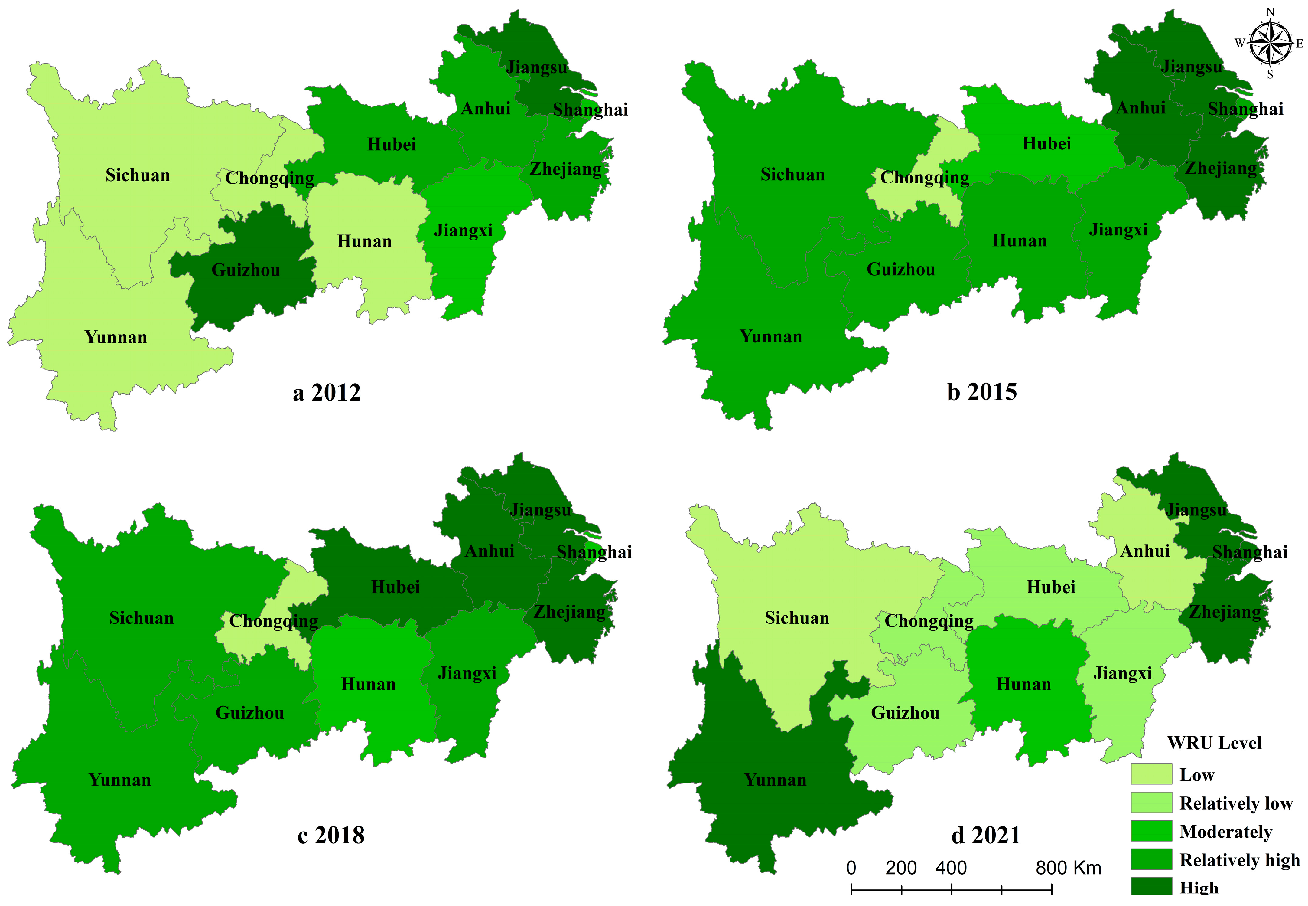
3.2. Characteristics of the Spatial Evolution of the Performance Level of Subsystems in the YREB

After measuring the overall WRMP of the large-scale regional units, to gain a better understanding of the spatial distribution pattern of the management performance level of each subsystem in the YREB, according to the data obtained from the measurement, 2012, 2015, 2018, and 2021 were selected as the observation time points, and Arcgis was then used to visualize the WRMP level of each subsystem in the 11 provinces (cities) of the YREB. Figure 4, Figure 5 and Figure 6 display the outcomes of the evolution.

(1)

Overall, the provincial WRU performance level in the YREB varies significantly between 2012 and 2021, exhibiting a “inverted U” pattern of development that initially increases and then decreases. Spatially, the WRU performance was high in the eastern provinces and low in the western provinces, whereas the WRU performance of Yunnan Province showed a continuous improvement. Locally, the WRU performance of Chongqing was poor and only marginally improved in 2021, whereas the WRU performance in the Yangtze River Delta region was excellent.

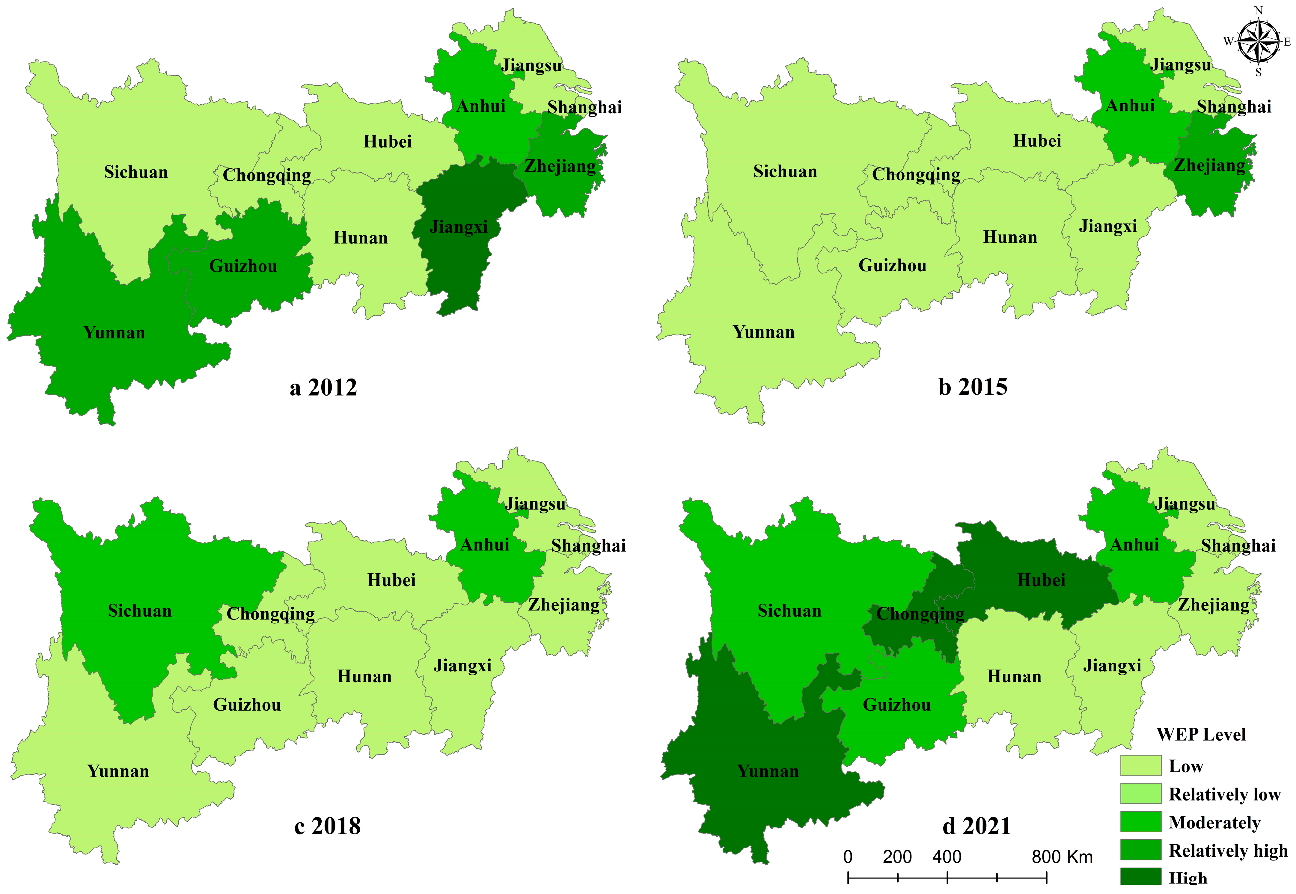
(2)

Overall, between 2012 and 2021, the WET performance level became better from the west to the east. Among these, the proportion of provinces with low and relatively low values was decreasing, while the proportion of provinces with moderate values and above was increasing. The provinces with moderate values and above were roughly characterized by “scattered distribution–group distribution–connected distribution”. In 2012, the proportion of provinces with median and above WET performances was 45%, while the proportion of provinces with median and above performances had reached 91% by 2021. Locally, the WET performances of Sichuan, Hubei, Hunan, Jiangxi, and the provinces in the Yangtze River Delta region showed continuous improvements, while the WET performances of Yunnan, Guizhou, and Chongqing showed fluctuating states.

(3)

Overall, the WEP performance level in the YREB from 2012 to 2021 was generally poor, and the difference between provinces was minimal. However, the WEP performance level became better with time. Specifically, the WEP performance levels in Jiangsu and Shanghai were at relatively low levels. Anhui Province was at a moderate performance level. The WEP performance levels in Zhejiang, Jiangxi, and other provinces were gradually decreasing, while the WEP performance levels in Hubei, Sichuan, and Yunnan Province were continuously improved.

3.3. Analysis on the Influencing Factors of WRMP Level in the YREB

Water resources management is an intricate task, and its effectiveness is determined by the collaboration of its several elements. In this paper, the factor detector and interaction detector in the geographic detector model were utilized to identify the influencing factors of the WRMP level in the YREB. The K-means clustering technique was applied to discretize the 23 indexes’ data, and then the data were imported into the geographic detector.

Table 5. Geographical detection results of influencing factors of WRMP level evolution.

Sort	2012		2015		2018		2021
	Single Factor	Interaction	Single Factor	Interaction	Single Factor	Interaction	Single Factor	Interaction
1	X2 (0.526 *)	X8∩X2 (0.859)	X2 (0.468 *)	X23∩X7 (0.859)	X20 (0.394 *)	X20∩X13 (0.982)	X11 (0.502 *)	X17∩X11 (0.975)
2	X7 (0.413 **)	X12∩X7 (0.834)	X18 (0.420 **)	X15∩X3 (0.855)	X7 (0.328 *)	X21∩X17 (0.982)	X3 (0.371 *)	X20∩X19 (0.975)
3	X20 (0.398 **)	X13∩X2 (0.827)	X9 (0.408 **)	X13∩X9 (0.834)	X21 (0.320 *)	X15∩X11 (0.964)	X4 (0.361 *)	X8∩X1 (0.967)
4	X17 (0.390 **)	X17∩X7 (0.824)	X20 (0.378 *)	X15∩X7 (0.825)	X19 (0.320 *)	X21∩X20 (0.964)	X22 (0.284 *)	X20∩X12 (0.967)
5	X1 (0.383 **)	X19∩X7 (0.819)	X3 (0.356 **)	X13∩X7 (0.793)	X1 (0.319 *)	X13∩X8 (0.955)	X20 (0.227 *)	X2∩X1 (0.942)
6	X8 (0.362 **)	X17∩X3 (0.808)	X5 (0.345 *)	X6∩X3 (0.781)	X9 (0.317 *)	X21∩X13 (0.943)	X16 (0.204 *)	X11∩X1 (0.942)
7	X23 (0.309 *)	X20∩X2 (0.806)	X4 (0.279 *)	X20∩X17 (0.774)	X17 (0.304 *)	X9∩X1 (0.935)	X18 (0.184 *)	X21∩X1 (0.942)
8	X5 (0.262 *)	X9∩X7 (0.805)	X1 (0.193 *)	X20∩X13 (0.769)	X3 (0.298 *)	X11∩X6 (0.920)	X17 (0.160 *)	X3∩X2 (0.900)

Note: $X_i(i=1, 2,\cdots 23)$ represents each evaluation index; the numbers in parentheses represent the $q$ value corresponding to the impact factor; * $p<0.1$, ** $p<0.05$.

displays the outcomes of the single factor and interaction detection. Due to space reasons, the table only lists the top eight factors explained by the single factor explanatory power and interaction in 2012, 2015, 2018, and 2021.

From the results of single factor detection, overall, X2, X3, X7, X8, X9, X11, X20, and X21 were found to have the highest q mean values in the four observation years, with the industrial water saving rate, water resources development and utilization rate, water resources sustainability index, sewage diameter ratio, urban water penetration rate, industrial wastewater treatment completion rate, ecological construction and protection of the year to complete the investment in GDP, and the growth rate of water ecological carrying capacity being the most influential indicators of the WRMP level. Apart from the industrial wastewater treatment completion rate, the remaining seven factors belong to the two subsystems of the WRU and WEP. Therefore, when striving to raise the WRMP level, it is necessary to focus on the sequences of the WRU, WEP, and WET subsystems. Locally, between 2012 and 2021, only two factors, the industrial water saving rate and industrial wastewater treatment completion rate, had q values higher than 0.5, and the effect of the other elements varied significantly each year and was lower than 0.5. It is evident that, in order to enhance the WRMP level, various factors must be adjusted over time.

The results of the interaction detection showed that there was a significant interaction between the factors, indicating that the interaction of influencing factors has a promoting effect on the improvement of the WRMP. Overall, the interaction types between each influencing factor were mainly nonlinear enhancement and two-factor enhancement. Specifically, in 2012, among the interaction types between the two influencing factors, there were more nonlinear enhancement relationships than the number of two-factor enhancements. After the interaction, the top eight interaction factors had a higher explanatory power than that of a single factor. Among them, X8∩X2 (0.859) and X20∩X2 (0.806) belonged to the two-factor enhancement type, and the rest belonged to the nonlinear enhancement type. In 2015, after interacting with the other factors, the water resources sustainability index (X7) and the sewage treatment rate (X13) significantly increased in explanatory power, and the top eight interaction factors of explanatory power belonged to the type of nonlinear enhancement after the interaction. This demonstrated that the combination of several influencing elements resulted in the establishment of the spatial differentiation pattern of the WRMP level in the YREB. In 2018, the interaction between the proportions of completed investment in ecological construction and protection in GDP (X20) and the sewage treatment rate (X13) were the strongest. The $q$ value after the interaction was 0.982, and the type of action was nonlinearly enhanced. In addition, compared with the single-factor detection results, it can be found that the explanatory power of the top eight factors in the single-factor detection was weak and within 0.4, but after the interaction, the explanatory power of the top eight factors was higher than 0.9. Accordingly, the interaction between various factors had a significant impact on the spatial differentiation of the WRMP. In 2021, the explanatory power of the interaction between the agricultural fertilizer application intensity (X17) and industrial wastewater treatment completion rate (X11) was as high as 0.975. All of the interaction types were nonlinear enhancement. In addition, 50% of the top eight factors of the interaction are related to the per capita water use (X1) factor, indicating the importance of per capita water use capacity for water resources management.

4. Discussions

4.1. Comparative Analysis of WRMP Evaluation

(1)

From 2012 to 2021, the WRMP level in each province of the YREB showed a continuously improved trend. The conclusion of this result is consistent with the proposal and background of some policies, such as the Opinions on the Implementation of the Strictest Water Resources Management System, which was issued by the State Council in 2012; the Opinions of the Central Committee of the Communist Party of China and the State Council on Comprehensively Strengthening the Protection of Ecological Environment and Resolutely Fighting the Battle of Pollution Prevention and Control, which were issued in 2018; and the Fourteenth Five-Year Plan for the Supervision and Management of Ecological Environment Protection, which was issued in 2021. The implementation of these policies had a huge impact and significantly enhanced the WRMP level in the YREB. A comparison reveals that Zhejiang Province’s WRMP level has consistently been among the highest. This is due to Zhejiang Province’s strong natural resources foundation and its impressive accomplishments in water conservation, emission reduction, and pollution control, which have successfully eased the conflict between the availability and demand for water resources. However, Shanghai has the worst WRMP level, and its high population density, high degree of urbanization, high demand for urban and industrialized water, and ineffective pollution control are the causes of this. Furthermore, the implementation of the Water Pollution Prevention Action Plan in 2015 allowed certain provinces to enhance the effectiveness of water resources utilization and fortify the oversight of water environment administration. This explains why, since 2016, the WRMP levels in the Anhui, Jiangxi, Hubei, and Sichuan provinces have significantly improved. In contrast, some scholars [49] by combining a data envelopment analysis (DEA) and the Malmquist index model, discovered that the national WRMP level showed an upward trend from 2013 to 2019. This finding was somewhat similar with the conclusions of this paper.

(2)

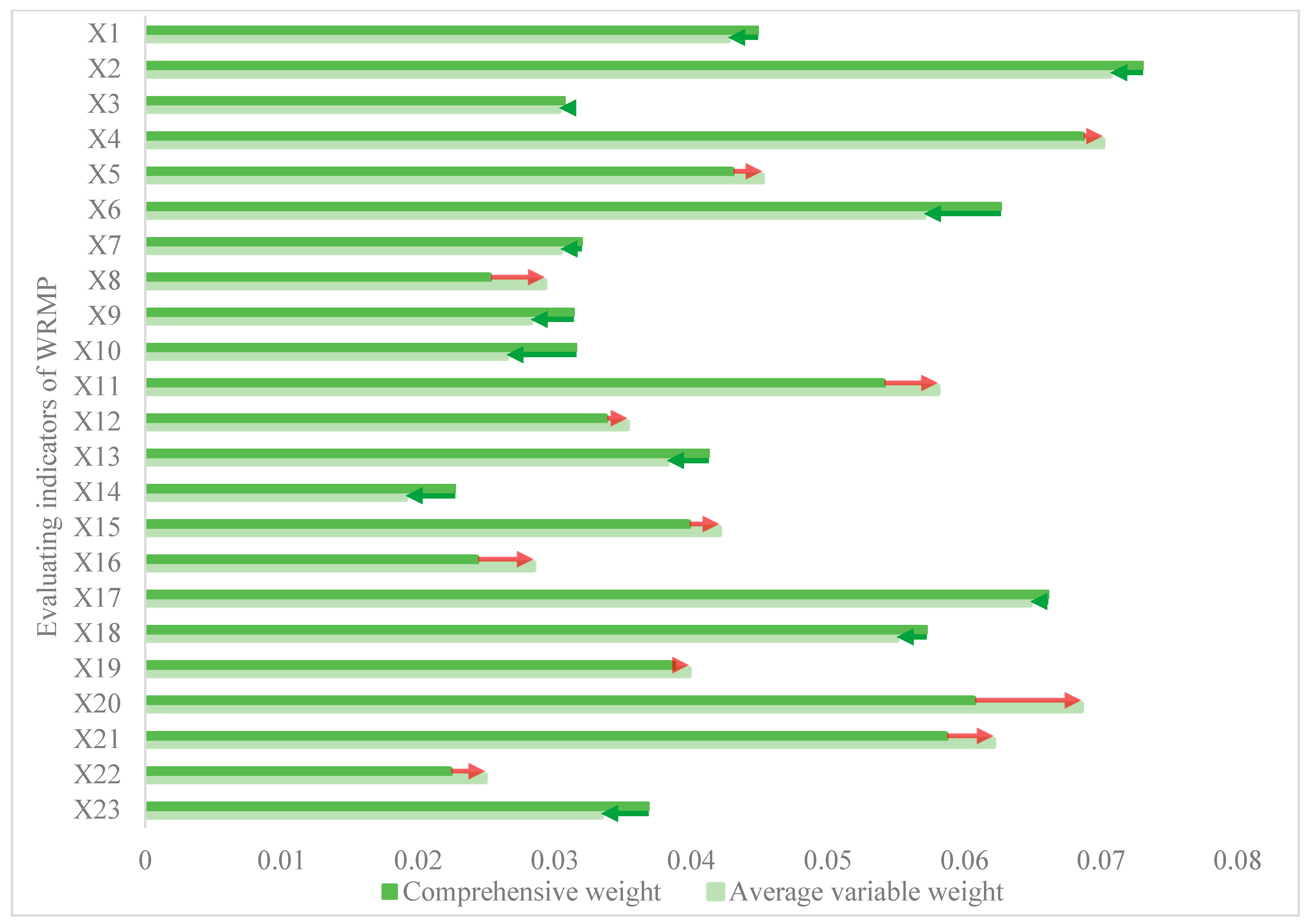
The evaluation results of the matter–element extension model before and after the variable weight modification are generally consistent, but there will be subtle differences. The model after variable weight modification is closer to reality. This is mostly due to the fact that the variable weight theory adjusts the comprehensive weight based on the index’s actual value, increasing the accuracy of the evaluation results by bringing the weight closer to the index’s actual situation. As shown in Figure 7, the comprehensive weight is compared with the average value of the ten-year variable weight. It is discovered that the value of more indicators after weight modification is reduced, while the weights of indicators with more outliers will become larger, making the importance of the indicators more apparent. For this reason, through the two methods, we can find that the evaluation grades of Shanghai as well as Sichuan Province in 2012, after variable weight modification, are low, while the evaluation grade before the modification is relatively low, but there is a tendency for it to change to a low level. This phenomenon is due to the fact that the industrial wastewater treatment completion rate (C11), ecological construction and protection of this year to complete the investment accounted for the proportion of GDP (C20) in Shanghai (2012), and the utilization rate of water resources development (X3) in Sichuan (2012) had minimum values. The emergence of the minimum value makes the variable weight of these indicators increase, eventually leading to the WRMP evaluation level being reduced to a low level. Accordingly, the variable-weighted corrected evaluation results better reflect the actual situations.

(3)

In the management performance evaluation of each subsystem, first of all, the WRU performance is high in the east and low in the west. This is a result of the eastern region being economically developed and having high technical support in the economical and intensive use of water resources. On the other hand, Liu and Liu (2023) [50] applied the super-efficiency data envelopment analysis model (SE-DEA), combined with the total factor productivity index (DEA-Malmquist), and discovered that the WRU center of gravity in the YREB (2011—2020) shifted from northeast to southwest and was situated east of the geographical center of gravity. This demonstrates that the east’s WRU performance is superior to that of the west. Nonetheless, the gap between the WRU performance in the east and the west is progressively narrowing, which is basically consistent with the content of this paper. Furthermore, in recent years, the state has strengthened the WET policy of the YREB, enhanced the WET in the upper reaches of the Yangtze River, and addressed the issue of wastewater discharge treatment in the upper reaches of the Yangtze River. As a result, the WET performance level has improved recently and showed an improved trend from the Western Region to the Eastern Region. Finally, Shanghai and Jiangsu Province performed relatively poorly in terms of the WEP, which may be closely related to the population density, industrial water intensity, and ecological environment water consumption in these two places.

The national ecological protection strategy in the upper reaches of the YREB has been improving, which is why the WEP performances of Yunnan and Sichuan have been becoming consistently better.

The capacity for water ecological restoration was enhanced. After 2018, the WEP performances in Chongqing, Hubei, and other locations has been progressively elevated to high values. This might be the case, since Hubei and Chongqing consistently enhance the ecosystem’s recreational value while preserving its authenticity under the strategic direction of China’s ecological preservation. In contrast, some scholars [51] considered that the water ecological performances of Hubei and Chongqing are at moderate levels, which is slightly different from the results of this paper.

4.2. Identification of Main Influencing Factors of WRMP Level

The WRMP evaluation can assess the efficacy of water resources management from various perspectives and efficiently oversee and consistently enhance its management means [52]. Hence, it is essential to explore its main influencing factors. Currently, numerous studies have been conducted to investigate the factors that impact the WRU efficiency, yet few studies have been conducted on the influencing factors of the WRMP. Consequently, this paper employs the geographical detector model to detect the factors that have a greater impact on the WRMP level. First of all, based on the findings of the single-factor detection, the top eight factors with larger $q$ mean values were the industrial water saving rate (0.497), water resources development and utilization rate (0.342), water resources sustainability index (0.371), sewage diameter ratio (0.362), urban water penetration rate (0.362), industrial wastewater treatment completion rate (0.502), ecological construction and protection investment accounted for the proportion of the GDP this year (0.349), and the water ecological carrying capacity growth rate (0.320). Among them, the industrial wastewater treatment completion rate and the industrial water saving rate have a greater explanatory power. The mean value of q is approximately 0.5, indicating that these factors have a substantial impact on water resources management in the YREB. This is mainly because the YREB has attracted many industrial and mining enterprises due to its own resources and geographical advantages [53]. Industrial and mining enterprises will discharge a large amount of sewage while consuming a lot of water resources, which aggravates the difficulty of implementing water resources management in the YREB. Therefore, in order to effectively improve the WRMP in the YREB, it is necessary to implement the dual control of water resources utilization and treatment. That is to say, on the basis of improving the efficiency of industrial water use, the intensity of wastewater treatment should be continuously improved to achieve the efficient management of water resources. Secondly, from the perspective of the number of the top eight factors with greater influences, the influence of each subsystem, from high to low, are the WRU subsystem, the WEP subsystem, and the WET subsystem. This demonstrates that the sequence of the WRU, WEP, and WET subsystems should be taken into consideration when enhancing the WRMP. Ultimately, from the results of the interaction factor detection, it can be found that most of the single factors show nonlinear enhancement after the interaction. This outcome demonstrates that several variables must cooperate in order for the WRMP to be changed in the YREB.

4.3. Limitations and Future Research

This paper introduces the game variable weight matter–element extension model to quantitatively evaluate the WRMP level. Secondly, Arcgis and the geographical detector model are combined to analyze the spatial and temporal status of the WRMP and explore the important influencing factors affecting the WRMP level. Nevertheless, there are still certain shortcomings that merit more research. Firstly, in terms of index selection, the three aspects of water resources, water environment, and water ecology are considered. However, the phenomenon of “looking at the sea in the city” has become more frequent recently. While strengthening the construction of the drainage system, urban flood treatment should be included in the overall framework of basin water environment treatment. Secondly, while choosing indicators, this paper takes into account the availability of data, so indicators related to water resources biodiversity have not yet been selected. Therefore, future research should include pertinent indicators in this domain in the indicator evaluation system. Finally, due to the strong regional uniqueness and heterogeneity of WRMP evaluation, it is necessary to further judge whether it is universal in other research areas. Hence, in the future, WRMP evaluation should be carried out, and comparatively, classifications for regions with different characteristics should be studied.

5. Conclusions

In this paper, the game variable weight matter–element extension evaluation model was innovatively introduced into the field of large-scale basin WRMP evaluation, and the YREB was used as an example. Firstly, the overall WRMP from 2012 to 2021 was measured, and the results of the model before and after the variable weight modification were compared to verify the fit of the model used in this paper. Secondly, the spatial and temporal differentiation of each subsystem’s management performance in the YREB was analyzed. Finally, the geographical detector was used to explore the main factors affecting the WRMP in the YREB. Hence, this paper introduced a new evaluation model, which can also be used in other similar evaluation studies, such as water environmental carrying capacity and water ecological health. The main conclusions are as follows:

(1)

From 2012 to 2021, the overall WRMP level of each province in the YREB showed a continuously improved state. Among them, the WRU performance was high in the east and low in the west. The WET performance showed a trend of gradual improvement from the Western Region to the Eastern Region, while the WEP performance showed a gradual improvement trend.

(2)

The evaluation results of the game variable weight matter–element extension model were basically consistent with the evaluation results before the variable weight modification. There were only nuances in the WRMP level in Shanghai (2012) and Sichuan (2012), but the evaluation results of the variable weight-modified model were more fit to the actual situation.

(3)

According to the results of the geographical detector, the main factors affecting the WRMP level were different in different years. Consequently, to improve the WRMP level, it is necessary to target and adjust different factors in different years. Simultaneously, the interaction of impact factors had a nonlinear enhancement and a two-factor enhancement effect on the improvement of the WRMP.

References

1. Kong, Y.; He, W.; Gao, X.; Yuan, Y.; Peng, Q.; Li, S.; Zhang, Z.; Degefu, D.M. Dynamic assessment and influencing factors analysis of water environmental carrying capacity in the Yangtze River Economic Belt, China. Ecol. Indic. 2022, 142, 109214. [Google Scholar] [CrossRef]
2. Dost, R.; Kasiviswanathan, K.S. Quantification of Water Resource Sustainability in Response to Drought Risk Assessment for Afghanistan River Basins. NRRC 2023, 32, 235–256. [Google Scholar] [CrossRef]
3. Degefu, D.M.; He, W.; Yuan, L.; Zhao, J. Water Allocation in Transboundary River Basins under Water Scarcity: A Cooperative Bargaining Approach. WRM 2016, 30, 4451–4466. [Google Scholar] [CrossRef]
4. Sun, B.; Li, F. Water consumption patterns of 110 cities in the Yangtze River Economic Belt in 2015. Front. Earth. Sci. 2022, 10, 969991. [Google Scholar] [CrossRef]
5. Qin, C.; Guo, H.; Li, Y. Research progress on performance evaluation model of water resources management. Shanxi Water Conserv. Sci. Technol. 2021, 4, 50–52. [Google Scholar] [CrossRef]
6. Zhu, Y.; Jiang, S.; Han, X.; Gao, X.; He, G.; Zhao, Y.; Li, H. A Bibliometrics Review of Water Footprint Research in China: 2003–2018. Sustainability 2019, 11, 5082. [Google Scholar] [CrossRef]
7. Song, G. Evaluation on water resources and water ecological security with 2-tuple linguistic information. J. Knowl.-Based Intell. Eng. Syst. 2019, 23, 1–8. [Google Scholar] [CrossRef]
8. Zhao, J.; Zhao, Y. Synergy/trade-offs and differential optimization of production, living, and ecological functions in the Yangtze River economic Belt, China. Ecol. Indic. 2023, 147, 109925. [Google Scholar] [CrossRef]
9. Peng, Q.; He, W.; Kong, Y.; Yuan, Y.; Degefu, D.M.; An, M.; Zeng, Y. Identifying the decoupling pathways of water resource liability and economic growth: A case study of the Yangtze River Economic Belt, China. Environ. Sci. Pollut. Res. 2022, 29, 55775–55789. [Google Scholar] [CrossRef]
10. Yuan, L.; Yang, D.; Wu, X.; He, W.; Kong, Y.; Ramsey, T.S.; Degefu, D.M. Development of multidimensional water poverty in the Yangtze River Economic Belt, China. JEM 2023, 325, 116608. [Google Scholar] [CrossRef]
11. Xu, M.; Qin, S.; Ma, L. Review and prospect of water ecological environment protection: From pollution prevention and control to three-water coordination. Environ. Manag. China 2021, 13, 69–78. [Google Scholar] [CrossRef]
12. Bian, D.; Yang, X.; Wu, F.; Babuna, P.; Luo, Y.; Wang, B.; Chen, Y. A three-stage hybrid model investigating regional evaluation, pattern analysis and obstruction factor analysis for water resource spatial equilibrium in China. JCP 2022, 331, 129940. [Google Scholar] [CrossRef]
13. Elnaz, Z.; Reyhaneh, M.; Farhad, Y.; Mohammad, S.A.; Hugo, A.L. Investigation of water allocation using integrated water resource management approaches in the Zayandehroud River basin, Iran. JCP 2023, 395, 136339. [Google Scholar] [CrossRef]
14. Zhou, Y.; Li, B.; Han, J.; He, G.; Wang, K.; An, C.; Huang, Y. Enabling efficiency-driven and low-impact water management from robust decision making: A risk- and robustness-based multi-objective decision support model. JCP 2023, 394, 136277. [Google Scholar] [CrossRef]
15. Sandoval-Solis, S.; McKinney, D.C.; Loucks, D.P. Sustainability Index for Water Resources Planning and Management. Water Res. Plan. Manag. 2011, 137, 381–390. [Google Scholar] [CrossRef]
16. Zhou, S.; Xu, X.; Jia, C.; Zhu, J. Research on the application of improved principal component analysis in the comprehensive evaluation of regional water resources. China Rur. Water Cons. Hydr. 2014, 38, 1928–1933. [Google Scholar] [CrossRef]
17. Xu, H. A regional water resources management performance evaluation model and empirical research. People Yellow River 2016, 38, 42–45. [Google Scholar] [CrossRef]
18. Pan, H.; Xu, Q. Quantitative Analysis on the Influence Factors of the Sustainable Water Resource Management Performance in Irrigation Areas: An Empirical Research from China. Sustainability 2018, 10, 264. [Google Scholar] [CrossRef]
19. Reddy, M.J.; Kumar, D.N. Performance evaluation of elitist-mutated multi-objective particle swarm optimization for integrated water resources management. J. Hydroinformatics 2009, 11, 79–88. [Google Scholar] [CrossRef]
20. Huang, X.; Zhong, J.; Fang, G.; Chen, Y. Evaluation of water resources management modernization based on physical element analysis method. Adv. Water Res. Hydrop. Sci. Techn. 2017, 37, 22–28. [Google Scholar] [CrossRef]
21. Shan, C.; Dong, Z.; Lu, D.; Xu, C.; Wang, H.; Ling, Z.; Liu, Q. Study on river health assessment based on a fuzzy matter-element extension model. Ecol. Indic. 2021, 127, 107742. [Google Scholar] [CrossRef]
22. Ren, H.; Zhao, C.; An, L. Performance Evaluation of Minqin Oasis Water Resources Management Policy Based on the Mutation Level Method. Res. Sci. 2014, 36, 922–928. [Google Scholar]
23. Wu, D.; Wang, Y.H. Dynamic evaluation of integrated water resources management performance in seven major river basins in China. Reso. Envir. Yangtze Basin. 2014, 23, 32–38. [Google Scholar] [CrossRef]
24. Guo, W.; Zuo, Q.; Jin, R.; Ma, J. Performance assessment system and application of strictest water resources management in Zhengzhou. South North Water Divers. Water Sci. Technol. 2014, 12, 86–91. [Google Scholar] [CrossRef]
25. Smout, I.K.; Gorantiwar, S.D. Performance assessment of irrigation water management of heterogeneous irrigation schemes: 2. A case study. Irrig. Drain. Syst. 2005, 19, 37–60. [Google Scholar] [CrossRef]
26. Bumbudsanpharoke, W.; Prajamwong, S. Performance Assessment for Irrigation Water Management: Case Study of the Great Chao Phraya Irrigation Scheme. Irrig. Drain. 2015, 64, 205–214. [Google Scholar] [CrossRef]
27. Rieckermann, J.; Daebel, H.; Ronteltap, M.; Bernauer, T. Assessing the performance of international water management at Lake Titicaca. Aquat. Sci. 2007, 68, 502–516. [Google Scholar] [CrossRef]
28. Rey, J.; Tengnäs, A.; Lévite, H.; Ouédraogo, I. Integrated water resources management performance analysis: Results of a pilot study in West Africa. Water Supply Res. Techn. 2014, 63, 661–670. [Google Scholar] [CrossRef]
29. Molinos-Senante, M.; Hernández-Sancho, F.; Mocholí-Arce, M.; Sala-Garrido, R. A management and optimization model for water supply planning in water deficit areas. Hydrol. 2014, 515, 139–146. [Google Scholar] [CrossRef]
30. Zhou, K. Comprehensive evaluation on water resources carrying capacity based on improved AGA-AHP method. Appl. Water Sci. 2022, 12, 103. [Google Scholar] [CrossRef]
31. Wu, X. Economic Benefit Evaluation of Water Resources Recycling Utilization based on Analytic Hierarchy Process. JCR 2020, 104, 6–9. [Google Scholar] [CrossRef]
32. Li, S.; Sun, A. Evaluation and Prediction of Water Resources Based on AHP. In Proceedings of the 2016 International Conference on Environmental Engineering and Sustainable Development (CEESD 2016), Sanya, China, 9–11 December 2016; Volume 51. [Google Scholar] [CrossRef]
33. Yang, H.; Fu, K.; Sun, X. Comprehensive evaluation of water resources carrying capacity in Yantai City based on CRITIC-GR-TOPSIS method. Soil Water Conserv. Bull. 2021, 41, 215–221. [Google Scholar] [CrossRef]
34. Zhu, J.; Feng, J.; Gao, Y. Comprehensive evaluation model of happy rivers and lakes based on BWM-CRITIC-TOPSIS. Water Conserv. Hydropower Technol. Prog. 2022, 42, 8–14+20. [Google Scholar]
35. Wang, M.; Ye, C.; Zhao, L. Research on the evaluation of regional industrial science and technology innovation ability based on CRITIC and TOPSIS. J. Shanghai Univ. Sci. Technol. 2020, 42, 258–268. [Google Scholar] [CrossRef]
36. Liu, Y.; Hu, Y.; Hu, Y.; Gao, Y.; Liu, Z. Water quality characteristics and assessment of Yong ding New River by improved comprehensive water quality identification index based on game theory. Envir. Sci. 2020, 104, 40–52. [Google Scholar] [CrossRef] [PubMed]
37. Jiang, T.; Yao, C.; Tong, Z. Fuzzy comprehensive evaluation of subway shield construction safety management based on game theory combination weighting. J. North China Inst. Sci. Technol. 2021, 18, 86–92. [Google Scholar] [CrossRef]
38. Li, H. Mathematical Framework of Factor Space Theory and Knowledge Representation (VIII)—Variable Weight Synthesis Principle. Fuzzy Syst. Math. 1995, 2, 1–9. [Google Scholar]
39. Cai, W. Extension theory and its application. CSB 1999, 44, 1538–1548. [Google Scholar] [CrossRef]
40. Wang, Q.; Li, S.; Li, R. Evaluating water resource sustainability in Beijing, China: Combining PSR model and matter-element extension method. JCP 2018, 206, 171–179. [Google Scholar] [CrossRef]
41. Han, H.; Li, H.; Zhang, K. Urban Water Ecosystem Health Evaluation Based on the Improved Fuzzy Matter-Element Extension Assessment Model: Case Study from Zhengzhou City, China. MPE 2019, 2019, 7502342. [Google Scholar] [CrossRef]
42. Fan, Y.; Liu, T.; Li, T.; Jiao, W. Application of physical element analysis in the evaluation of water quality in the Yellow River. Water Res. Water Engin. 2013, 24, 166–169. [Google Scholar]
43. Balducci, F.; Ferrara, A. Using urban environmental policy data to understand the domains of smartness: An analysis of spatial autocorrelation for all the Italian chief towns. Ecol. Indic. 2018, 89, 386–396. [Google Scholar] [CrossRef]
44. Zhang, J.; Zhang, K.; Zhao, F. Research on the regional spatial effects of green development and environmental governance in China based on a spatial autocorrelation model. SCED 2020, 55, 1–11. [Google Scholar] [CrossRef]
45. Sun, D.; Gu, J.; Chen, J.; Xia, X.; Chen, Z. Spatiotemporal differentiation and influencing factors of urban water supply system resilience in the Yangtze River Delta urban agglomeration. Nat. Hazards 2022, 114, 101–126. [Google Scholar] [CrossRef]
46. Wang, J.; Xu, C. Geodetector: Principles and Prospects. Princ. Appl. Geogr. Detect. 2017, 72, 116–134. [Google Scholar] [CrossRef]
47. Deng, J.; Ye, S.; Xu, Z. Spatio-temporal analysis of ecological footprint and ecological carrying capacity of water resources in southeastern Sichuan. Rural. Water Conserv. Hydropower China 2023, 4, 125–133. [Google Scholar] [CrossRef]
48. Shen, S.; Wang, D.; Wang, Y. Combined weight-MNCM method for comprehensive evaluation of water resources carrying capacity. J. Nanjing Univ. Nat. Sci. 2021, 57, 887–895. [Google Scholar] [CrossRef]
49. Li, W.; Zou, Q.; Jiang, L.; Zhang, Z.; Ma, J.; Wang, J. Evaluation of Regional Water Resources Management Performance and Analysis of the Influencing Factors: A Case Study in China. Water 2022, 14, 574. [Google Scholar] [CrossRef]
50. Liu, Y.; Liu, S. Spatial-Temporal Evolution and Driving Factors of Water Resources Use Efficiency in Yangtze River Economic Belt. J. Wuhan Univ. Eng. 2023. Available online: http://kns.cnki.net/kcms/detail/42.1675.T.20230410.1230.002.html (accessed on 6 June 2023).
51. Xu, Y.; Yang, L.; Zhang, C.; Zhu, J. Comprehensive assessment and regional difference of water eco-environment in Yangtze River economic Belt. Soil Water Conserv. Bull. 2023, 43, 253–262. [Google Scholar] [CrossRef]
52. Zhu, H.; Wang, Z.; Liu, T. Performance Evaluation of Water Asset Management in China. Appl. Mech. Mater. 2011, 71–78, 2116–2121. [Google Scholar] [CrossRef]
53. Kong, Y.; He, W.; Yuan, L.; Zhang, Z.; Gao, X.; Zhao, Y.; Degefu, D.M. Decoupling economic growth from water consumption in the Yangtze River Economic Belt, China. Ecol. Indic. 2021, 123, 107344. [Google Scholar] [CrossRef]
Figure 1. Status of water resources in the YREB, China. Note: The higher the height of the histogram, the more extreme the water shortage state. According to the internationally recognized water shortage standard, this study is divided into five levels. In the first level, the per capita water resources are higher than 3000 m3, which represents a normal state without water shortage. In the second level, the per capita water resources are less than 3000 m3, which represents mild water shortage. The third grade is lower than 2000 m3, which represents a moderate water shortage state. The fourth grade is less than 1000 m3, which represents a serious water shortage state. The fifth level is less than 500 m3, which represents an extreme water shortage state.
Sustainability 16 00649 g001
Figure 2. Weight determination flow chart.
Sustainability 16 00649 g002
Figure 3. The level of provincial WRMP in the YREB (2012–2021).
Sustainability 16 00649 g003
Figure 4. Spatial distribution of WRU in the YREB in the 2012–2021 period.
Sustainability 16 00649 g004
Figure 5. Spatial distribution of WET performance levels in the YREB in the 2012–2021 period.
Sustainability 16 00649 g005
Figure 6. Spatial distribution of WEP performance levels in the YREB in the 2012–2021 period.
Sustainability 16 00649 g006
Figure 7. Evaluation index weight change comparison chart.(Note: The green arrow to the left represents that the average variable weight of the index in ten years is less than its comprehensive constant weight part; the red arrow to the right represents the part of the average variable weight of the indicator in the ten years that is greater than its comprehensive constant weight.)
Sustainability 16 00649 g007