Article

Estimating the Past and Future Trajectory of LUCC on Wetland Ecosystem Service Values in the Yellow River Delta Region of China

1
School of Civil Engineering and Geomatics, Shandong University of Technology, Zibo 255000, China
2
Guangzhou Institute of Geography, Guangdong Academy of Sciences, Guangzhou 510070, China
3
Key Laboratory of Land Surface Pattern and Simulation, Institute of Geographical Sciences and Natural Resources Research, Chinese Academy of Sciences, Beijing 100101, China
4
Satellite (Shandong) Technology Group Co., Ltd., Jinan 250031, China
*
Authors to whom correspondence should be addressed.
Sustainability 2024, 16(2), 619; https://doi.org/10.3390/su16020619
Submission received: 22 November 2023 / Revised: 26 December 2023 / Accepted: 8 January 2024 / Published: 10 January 2024
(This article belongs to the Special Issue Climate Change and Enviromental Disaster)

Abstract

:
Land use/cover change (LUCC) can impact the provision of ecosystem service values (ESVs), particularly in wetland regions that are subject to frequent and unsustainable land conversions. Exploring the past and future trajectory of LUCC and its effects on ESV has a great significance for wetland management and habitat stability. This study tried to reveal the patterns and magnitude of LUCC on ESV under varying land development scenarios in the Yellow River Delta region, which is a typical region undergoing serious degradation in China. In this study, a combined approach utilizing equivalent coefficients of ecosystem services was employed to determine the ESV of the wetland in relation to the major land use types (LUTs). The Markov–FLUS model was then used to simulate LUTs across multiple scenarios in 2030 and to clarify the relationship of ESV between wetland and other LUTs. The results indicated that the wetland was severely degraded, with a loss in area of 6679.89 ha between 2000 and 2020. Cropland and water body were the main sources of diversion and turnover for the wetland, respectively. Despite the multiple scenario projections revealed, the wetland area exhibited a similar growth rate and a homogeneity in ESV under the natural development (ND), urban construction and development (UCD), and the ecological development (ED) scenarios. The ED scenario was deemed the optimal development strategy for the wetland ecosystem. Our research will improve the comprehension of land development decisions and promote sustainable development in estuarine wetland areas.

1. Introduction

The meaning of ecosystem services (ESs) is the ecological functions from which peoples can attain diverse benefits in various natural ecosystems [1,2,3]. Ecosystem service values (ESVs) apply economic rules to estimate ESs and transform them into practical applications [4,5]. Wetlands play a crucial role in contributing to the global stability of ecosystems. Globally, more than 23% of the annual ESV is provided by wetlands [6]. However, as human activities intensify and bring about the loss of biodiversity and unstable change in the global climate, numerous wetlands, especially estuarine wetlands, have been severely degraded. Half of the world’s wetlands have disappeared since 1900, leading to a decline in their value and function [7,8]. Land use/cover change (LUCC) has a momentous influence on the provision of ES. Therefore, it is essential to examine the history and future trajectory of LUCC and its effects on ESV in order to make informed decisions on land development and achieve sustainable development in wetland regions [9,10].
Numerous works from the literature have probed the consequences of the land use conversion on ES through the analysis of land use types (LUTs) and ES assessment [11,12,13]. Originally, the current and former LUTs served as the basis for investigating the effects of LUCC on ESV [14,15]. Research on LUCC and its impact on ESV have primarily focused on evaluating the role of different LUTs in ESV [16,17], examining the drivers of ESV change by analyzing various LUTs in combination with natural and economic factors [18,19], and exploring trends in ESV changes due to the shifts in different LUTs [20,21]. These studies can facilitate the detection of spatial heterogeneity and trends in ESV, while the results are less practical for anticipating and mitigating future issues.
The modelling and prediction of land utilization can provide a scientific basis for future changes in ESV in wetland ecosystems. More and more land utilization models have been proposed and applied in the study of ESV, such as the cellular automata model, CA-Markov model, CLUE-S model, and so on [22,23]. However, these models can only simulate land utilization from quantity or space, and cannot take into account the impact of both on land utilization. To address this issue, the Markov–FLUS model has been developed and employed in several studies to simulate future patterns of land usage [24,25,26]. This method, which combines a roulette wheel selection mechanism and a neural network algorithm with the cellular automata (CA) model, can be achieved by generating an adaptive atlas that integrates a range of natural and social factors, and the impact on land utilization can be considered both quantitatively and spatially. Its results will make spatial trajectories more explicit, allowing for the simulation of various LUTs in different scenarios.
Based on the LUTs in a spatially explicit simulation, the utilization of biophysical models [27] and the equivalent-coefficient method [28] can be employed to evaluate future ESVs. The lack of available data hinders the use of biophysical models to predict ESV under alternative scenarios due to the need to parameterize many variables [29]. In contrast with biophysical models, equivalent-coefficient approaches predict ESVs more easily, with less data requirements and acceptable results [30]. As a result, these methods were widely used to assess changes in ESV in response to LUCC [31,32]. However, some ESV assessments using the equivalent-coefficient method assumed identical ESV per acre for a particular LUT without giving thought to the heterogeneity of ES for a particular LUT in diverse zones [33,34,35]. Therefore, it is crucial to establish appropriate guideline systems that are suitable for the generation of spatially explicit ESVs per unit area and allow for the analysis of spatial disparities in ESVs [36,37]. The adjusted equivalent-coefficient method allows for ESV calculations under data-limited conditions. Additionally, the Markov–FLUS model can simulate land utilization in both quantitative and spatial perspectives, enabling the prediction and assessment of ESVs accurately. These methods make it possible to study the impact of historical and future trajectories of LUCC on ESVs.
The wetland in the Yellow River Delta (YRD) is a unique estuarine ecosystem. Compared with other estuarine wetlands, due to the large amount of sediment carried by the Yellow River into the sea, a large number of shallows and wetlands will be formed at the confluence of the river and the sea, and the wetland changes are very frequent, which is exacerbated by human activities. In addition, considering the availability of data, the YRD was chosen as the study region. The study had three objectives: (1) to investigate the LUCC over the last 20 years in the study region and the pertinence between wetland and various LUTs; (2) to summarize the change pattern of ESVs under past LUCC conditions and determine wetland’s contribution to ESV; and (3) to analyze the influence of different development scenarios on the regional wetland ecosystem and overall LUTs. Exploring the history and future trajectory of LUCC and its effects on ESV will enhance the comprehension of estuarine wetland ecosystem development and regional ecological conservation.

2. Materials and Methods
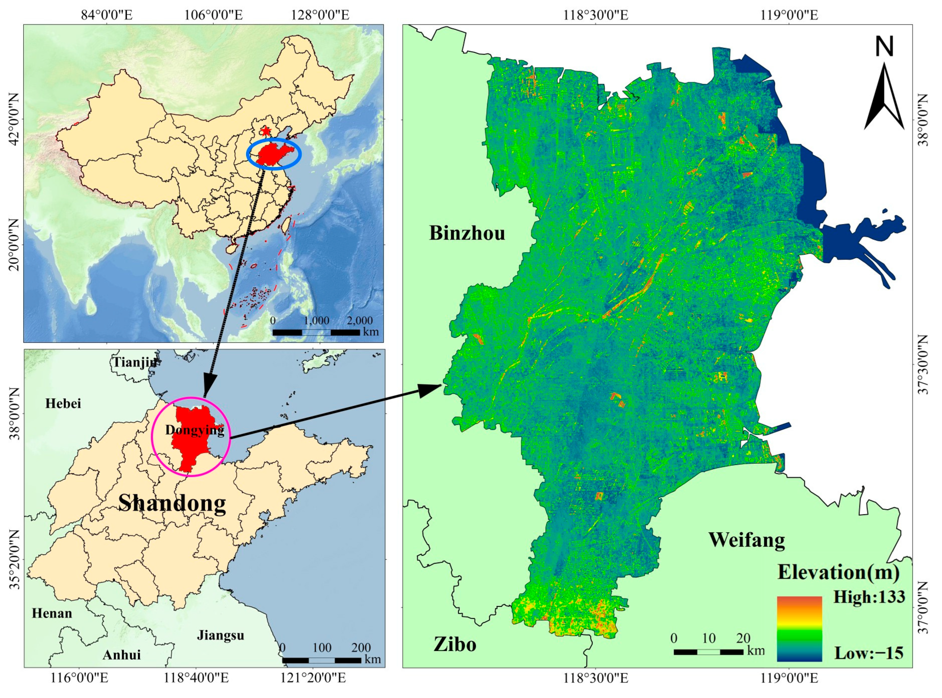
2.1. Study Area

The Yellow River Delta (YRD) is located between 118°33′~119°20′ E and 37°35′~38°12′ N, on the northern (Bohai Sea) coast of Shandong Province. It is mainly situated in Dongying (Figure 1). The climate of the region belongs to the temperate monsoon, with an annual temperature and precipitation of 12.8 °C and 555.9 mm, respectively. In accordance with the Shandong Bureau of Statistics, the population of Dongying was 2,193,500 at the end of 2020. The region’s GDP grew from CNY 46.511 million in 2000 to CNY 298.199 million in 2020. The area is an important petrochemical base in China, with topography that is lower in the northeast than in the southwest [38,39].
The protection and rejuvenation of wetlands are crucial for maintaining the security and biodiversity of the watershed ecosystem. YRD hosts a unique estuarine wetland ecosystem, which is rare on a global scale. However, the shortage of ecological water and other issues have resulted in a significant risk of deterioration. Studying the variation in ESVs in this region is of great significance for safeguarding and rehabilitating the wetland [40,41].

2.2. Data Collection and Preprocessing

The Data Sharing Service System (https://data.casearth.cn/ (accessed on 2 March 2023)) furnished the land utilization data with 30 m spatial resolution, the precision of land utilization classification for different years reached 82.5%, and the study showed that its classification products can meet the needs of applications at a global or regional scale [42]. In accordance with the data classification system and the current situation in the study region, the data were processed and classified into seven categories: artificial surface, cropland, bare land, forest, water body, wetland, and grassland. Six types of driving factors’ data were used in this study: DEM, road, temperature, precipitation, slope, and railways. The Resource and Environment Science and Data Center (https://www.resdc.cn/ (accessed on 2 March 2023)) furnished the administrative division of Dongying, road, and railway data. The data of the road and railway with 1 km spatial resolution and distances were calculated to roads and railways by using Euclidean distances in ArcGIS 10.2. Geospatial Data Cloud (https://www.gscloud.cn/ (accessed on 30 March 2023)) furnished the DEM data with 30 m spatial resolution. The slope data were obtained by processing the DEM data with ArcGIS 10.2. The China Meteorological Science Data Service Centre (https://data.cma.cn/ (accessed on 4 April 2023)) furnished the temperature and precipitation data with 1 km spatial resolution. The six driving factors were normalized using the Fuzzy Membership tool in ArcGIS 10.2. The Statistical Yearbook of China, Shandong, and Dongying furnish the socioeconomic data. The National Farm Product Cost–Benefit Survey furnished market prices for different grains in the study for various years.

2.3. Methods

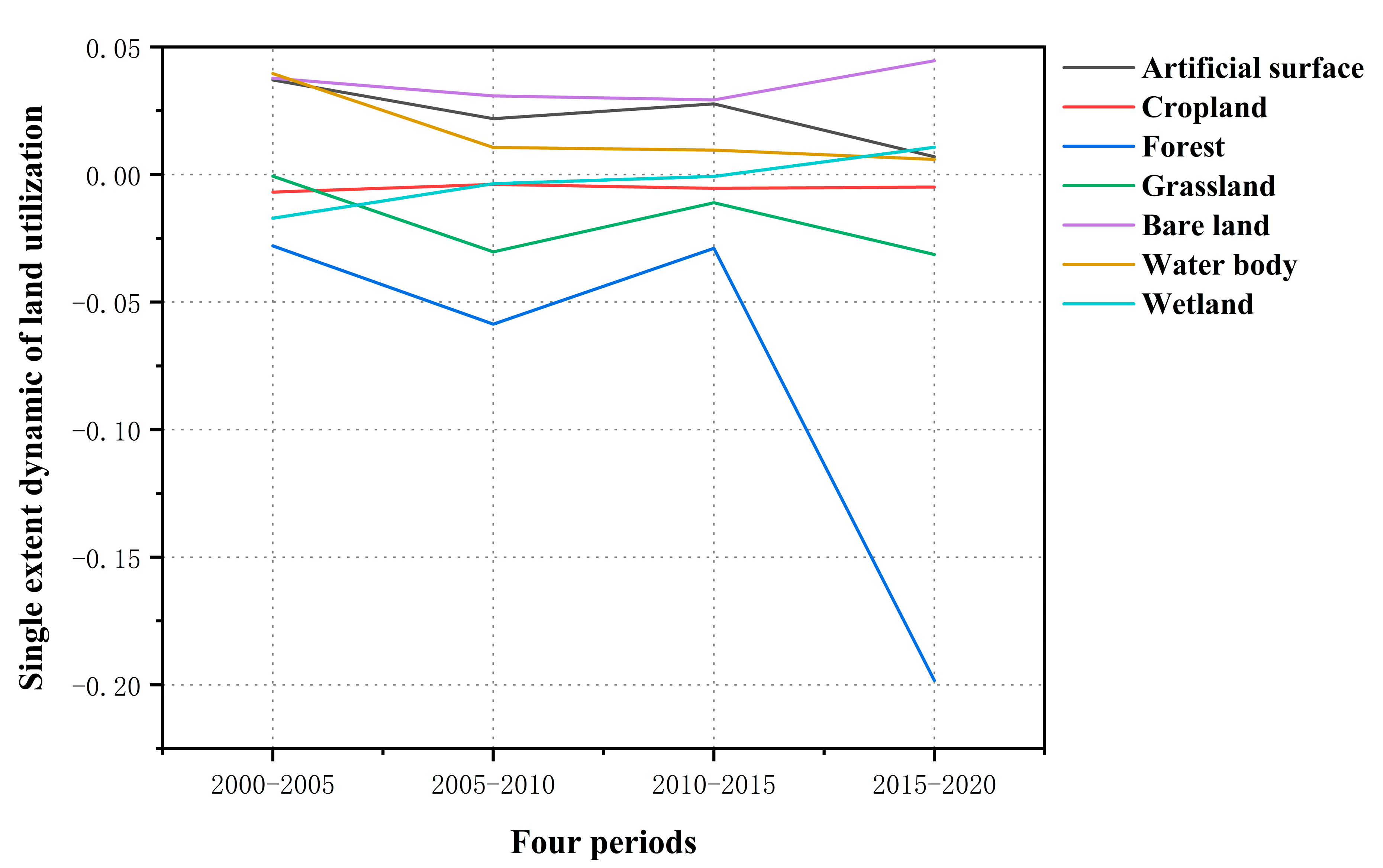
2.3.1. Extent Dynamic of Land Utilization

The intensity of transformation between various LUTs can be denoted as the integrated extent dynamic of land utilization [43]:
I D = i = 1 n U i n i U o u t i 2 i = 1 n U b i × 1 C × 100 %
where ID is the integrated extent dynamic of land utilization. Uin-i is the total of the other LUTs converted to LUT i over the course of the study. Uout-i is the total of LUT i converted to the other LUTs over the course of the study. Ubi is the area of LUT i at the initial phase of the study. C is the study period.
The LUTs’ change rate can be denoted as the single extent dynamic of land utilization [44]:
S D = G b G a G a × 1 H × 100 %
where SD is the single extent dynamic of land utilization. Ga is the area of a LUT at the initial phase of the study. Gb is the area of a LUT at the final phase of the study. H is the study period.

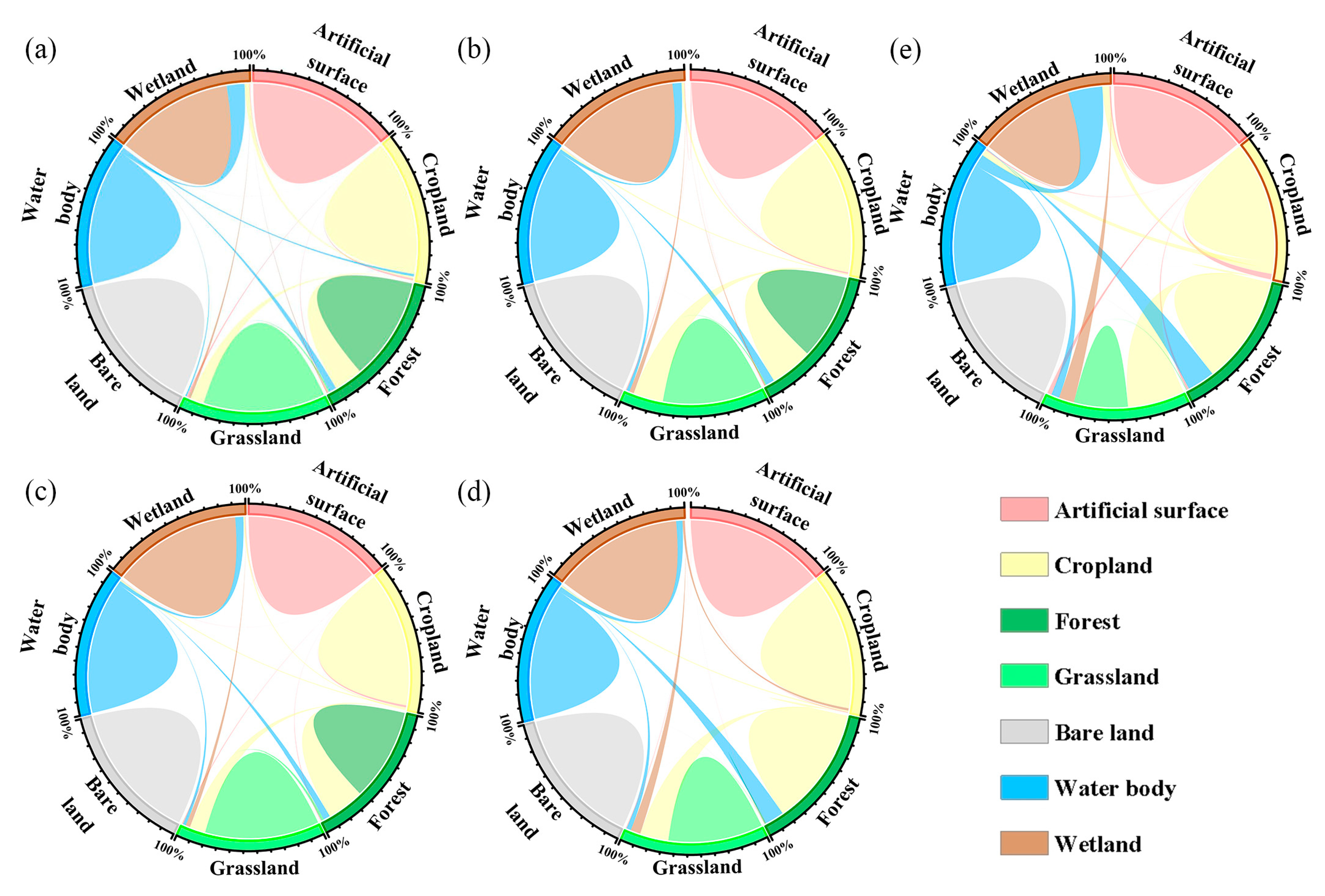
2.3.2. Land Use Transfer Matrix

The land use transfer matrix can describe the conversion relation between different LUTs and reveal information about transfer in and out of each LUTs [45]:
A i j = A 11 A 12 A 1 n A 21 A 22 A 2 n A n 1 A n 2 A n n
where Aij is the area of LUT i converted to LUT j over the course of the study (i, j = 1, 2, …, n). In this study, n is equal to 7.

2.3.3. Assessment of Ecosystem Service Values (ESVs)

For an accurate assessment of ESVs in the study region, the ecosystem service equivalent value was adjusted by socioeconomic data in the study region [46].
  • Adjustment of ecosystem service equivalent factor
Applying the ecosystem service equivalent factor of the other study region to the YRD in this paper would lead to inaccurate results [47]. The ecosystem service equivalent factor was adjusted by using a method based on food production per unit of area:
ε = N d N c
E i j = ε × E o i j
where ε is the regulatory factor. Nd is the harvested food per unit area in the study region. Nc is the harvested food per unit area in China. Eij is the ecosystem service equivalent factor of ES function j for LUT i after adjustment. Eoij is the ecosystem service equivalent factor of ES function j for LUT i before adjustment. The calculated ε is 1.06.
2.
The determination of ecosystem service value onset per hectare
The ESV per hectare is generally considered to be equal to one-seventh of the economic worth of grain harvested on a hectare of cropland at prevailing market prices. The main grain products in this study region are soybean, maize, and wheat [48]:
E x = n = 1 m u n v n s n A 7
where Ex is the ESV per hectare (CNY ha−1). The n is the grain type. The un (CNY ton−1) is the average market price of the nth grain. The vn (ton ha−1) is the average unit yield of the nth grain. The sn (ha) is the average area planted of the nth grain. The A (ha) is the area planted of all grains. The calculated Ex of YRD is 1425.33 CNY ha−1.
The coefficients on ecosystem service value were corrected using the method of food production per unit of area and the determination of ecosystem service value onset per hectare. Based on the ecosystem services equivalent factor table applicable to China [49] and equivalent-coefficient method, the regulatory factor, ESV per hectare, and ES value for different land utilization types applicable to the study were calculated. The adjusted coefficients are listed in Appendix A at the end of the manuscript, specifically in Table A1, Table A2 and Table A3.
3.
Calculation of ecosystem service values
The ESV is calculated using the benefit transfer method [50]:
Q i = j = 1 n E i j × E x
T E S V = i = 1 n Q i × S i
where Qi (CNY ha−1) is the ESV of one-hectare LUT i. Eij is the ecosystem service equivalent factor of ES function j for LUT i after adjustment. Ex is the ESV per hectare (CNY ha−1). TESV is the ESV in the region. The Si (ha) is the area of LUT i.

2.3.4. Markov–FLUS Model

  • Markov
The Markov model will automatically create the conversion probability matrix, the conversion area matrix, and the transition conversion of various LUTs [51]:
R ( s + 1 ) = P i j × R ( s )
P i j = P 11 P 12 P 1 n P 21 P 22 P 2 n P n 1 P n 2 P n n
where R(s + 1) is the land cover condition at time s + 1. R(s) is the land cover condition at time s. The Pij is the probability of conversion from the previous condition to the next condition.
2.
FLUS model
The FLUS model’s structure mainly consists of two parts [52].
(1) Probability calculation of land use distribution suitability based on neural network.
The Artificial Neural Network (ANN) is a feedforward neural network with a multilayer structure. Its effect is to train and predict the suitability probability of each LUT on a specific grid cell, which can be used to simulate the nonlinear complicated relationship between land use design and the drivers that are likely to influence their development.
(2) Adaptive cellular automaton and competition mechanism based on inertia.
The interaction of different LUTs is resolved by adaptive inertia and competition mechanisms. During the iterative procedure of the meta-automata, the combination probability of LUTs is estimated on each specific grid cells, and the ruling LUTs are assigned to the grid cell.
The Markov–FLUS model is a coupled model that works well for predicting future changes in LUTs.

2.3.5. Methods for Evaluating the Accuracy of Model Results

In this study, the kappa coefficient and figure of merit (FOM) were utilized to assess the simulation results. The kappa coefficient is commonly employed to assess the accuracy of classified or modeled data derived from remotely sensed images, with a focus on evaluating the data’s accuracy in terms of spatial location:
K = L p L q 1 L q
where K is the kappa coefficient. Lp is observation consistency, Lq is Lp is observational consistency. The calculated K is 0.8509, indicating a successful simulation, as it exceeded the threshold of 0.8 for good simulation [53].
The FOM method more effectively evaluated the metacells that underwent change, enhanced the accuracy assessment of the simulation, and proved to be more objective and realistic, particularly when the extent of land utilization change is relatively small compared to the total area of the study region.
F O M = R 2 R 1 + R 2 + R 3 + R 4
where R1 represents a region where change is observed, and the region remains unchanged during the simulation. R2 represents a region where change is observed, and the simulation correctly categorizes the region. R3 represents an area where change is observed, but the simulation assigns it to the wrong category. R4 indicates a region where no change was observed, but the simulation incorrectly changes the region. The calculated FOM value is 51.26%, which was below the standard range of 1% to 59%, and the accuracy rate increases with the increase in the FOM value [54].

3. Results

3.1. Spatial–Temporal Changes in Land Use

The major LUT in YRD was cropland, which constituted the highest average area of 62.28% in YRD from 2000 to 2020, followed by water body (16.23%), wetland (14.35%), and artificial surface (6.77%). Accordingly, grassland, bare land, and forest accounted for only 0.37% of the entire area. During 2000 to 2020, the land use trend displayed a significant decrease in cropland, forest, and grassland, accompanied by a significant increase in water body, artificial surface, and bare land (Table 1).
The noteworthy point is that the wetland, as the major LUT in YRD, was characterized by a trend of decrease, followed by an increase. From 2000 to 2015, the proportion of wetland decreased from 15.42% to 13.81%, and the area was reduced by 12,368.5 ha. The reduction in wetland area was predominantly in the northwestern part of the study region. Subsequently, between 2015 and 2020, the proportion of wetland increased to 14.55%, and the area increased by 5688.6 ha. The expansion of the wetland occurred in the estuary region (Figure A1), which has been designated as a National Ecological Reserve. The results indicated that the wetland, forest, and grassland are exhibiting a clear trend of degradation under normal development patterns, yet this deterioration can be slowed down or ameliorated through policy and human interventions.
The integrated extent dynamic of land utilization in the study region was 0.38% in 2000–2020. The forest, bare land, artificial surface, water body, and grassland exhibited a dramatic dynamic degree during the four periods of 2000–2005, 2005–2010, 2010–2015, and 2015–2020. However, there were relatively minor single extent dynamics of land utilization for these periods. The single extent dynamic of land utilization in the wetland was negative during the first three periods and positive across the last period. Alternately, positive and negative changes during the four periods resulted in a less pronounced single extent dynamic of land utilization in wetland across the entire study period (2000–2020) (Figure 2).
Throughout the entire period, the amount of cropland transferred out exceeded the amount of cropland transferred in, resulting in a reduction of 62,563.50 ha, or about 31.47%, 34.47%, and 33.11% of cropland converted to artificial surface, water body, and wetland, respectively (Figure 3). Artificial surface was dominated by the transferred in process during the period of 2000–2020, approximately 21,798.10 ha expansion from cropland (90.31%), wetland (5.75%), and water body (3.54%). During the same period, the water body experienced an expansion of about 51,101.45 ha, with 42.2% from cropland and 57.44% from wetland. Over the past twenty years, wetland conversion exhibited a relatively complex process involving both reduction and expansion. From 2000 to 2020, a total of 36,658.85 ha of wetland was transferred out, of which the proportions transferred to artificial surface, cropland, and water body are 3.42%, 16.15%, and 80.08%, respectively. At the same time, a total of 29,979.52 ha of wetland was transferred in, of which the proportions transferred in from artificial surface and water body are 69.10% and 29.87%, respectively. In general, the reduction in cropland and expansion of artificial surface and water body were the characteristics of the LUCC transformation in YRD. Moreover, the transformation of the wetland featured the complex conversions of the water body and cropland.

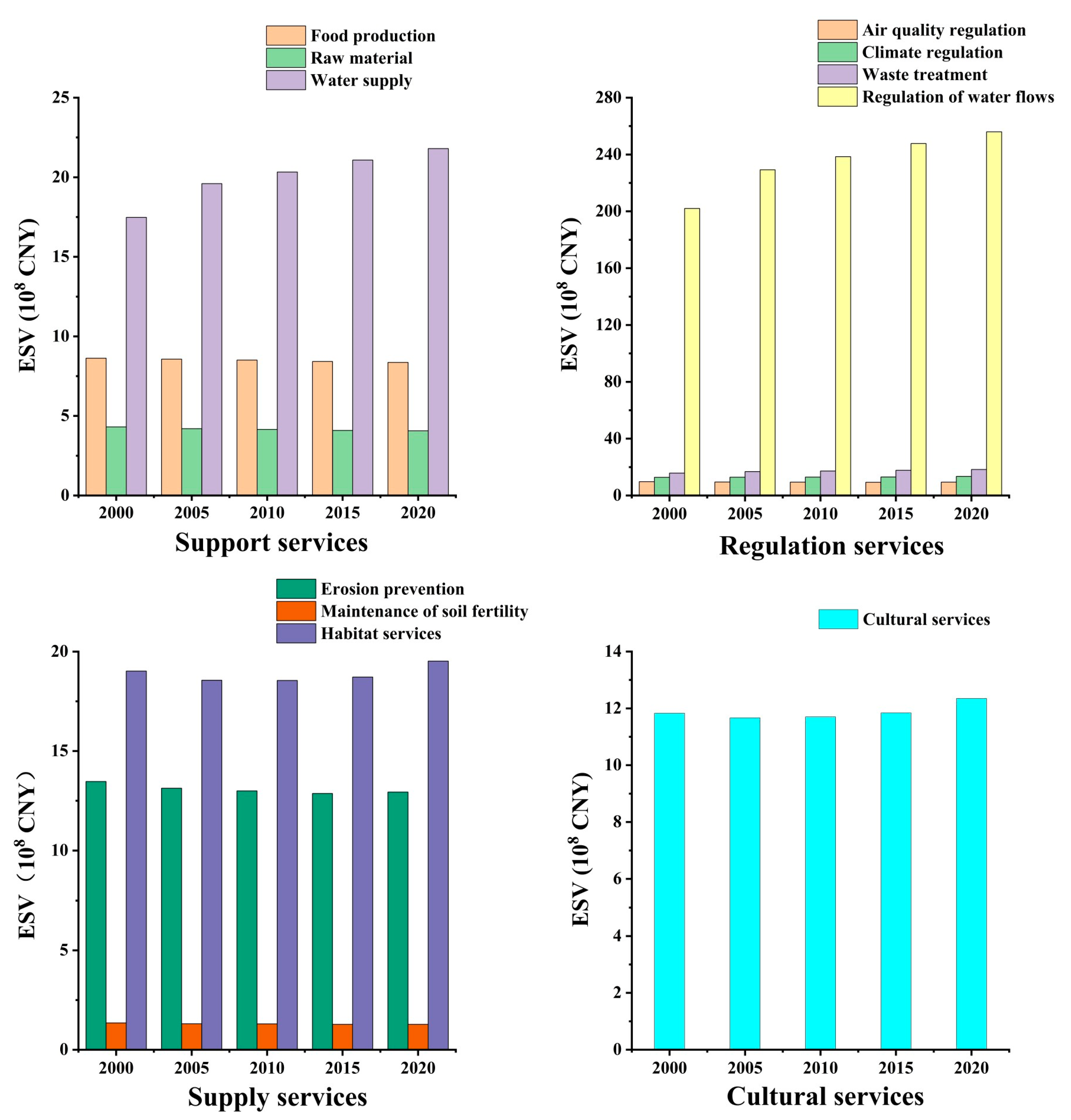
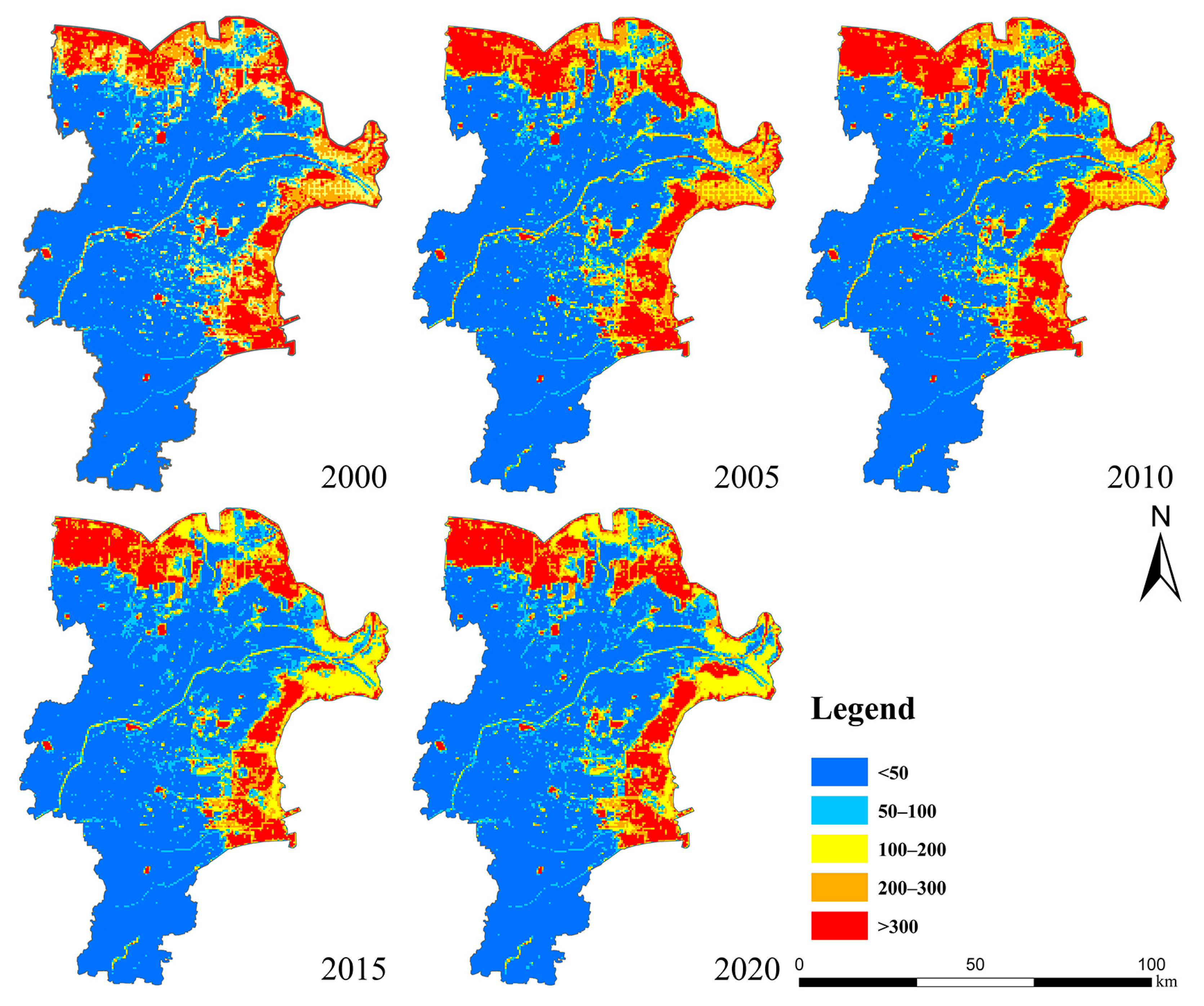
3.2. Spatial and Temporal Characteristics of ESV in YRD from 2000 to 2020

The total ESV in YRD increased from CNY 31.64 billion in 2000 to CNY 37.75 billion in 2020 (Table 2); there was a growth of 19.31%. The trends in the ESV can be divided into two periods: rapid growth (2000–2005) and slight growth (2005–2020). During the first period (2000–2005), the total ESV in the study region increased by about CNY 2.92 billion, there was a growth of 9.20%. In the second period (2005–2020), the total ESV increased by CNY 3.19 billion, with an average growth rate over three periods of 2.99%. During 2000 to 2020, the ESV of the wetland, cropland, grassland, and forest exhibited a slight reduction, decreasing by approximately CNY 0.53 billion, CNY 0.31 billion, CNY 16.74 million, and CNY 2.21 million, respectively. However, the ESV of the water body and bare land increased by CNY 6.96 billion and CNY 0.07 million, respectively. These findings suggested that the ESV exhibited faster growth during the initial phase, when land use changes occurred more frequently, but decelerated as the spatial arrangement of land use stabilized.
The ES function was divided into four first-level categories (FESs) and eleven second-level categories (SESs). In terms of the four FESs, the category of regulation services has the largest proportion of total ESV, exceeding approximately 75% during the 2000–2020 period. Consequently, the other three FESs, i.e., cultural services, support services, and supply services, offered smaller proportions of the total ESV, accounting for approximately 3.40%, 9.30%, and 9.50%, respectively. From the SES perspective, the largest ESC expansions were in the regulation of water flows, water supply, and waste treatment, amounting to 26.72%, 24.69%, and 16.64%, respectively. The expansion of these sectors was primarily linked to increases in the area of the water body. Meanwhile, the three SECs with the largest reduction were raw material, maintenance of soil fertility, and erosion prevention, with rates of −5.49%, −5.46%, and −3.97%, respectively. These decreases were mainly due to a decrease in cropland. Wetland contributed most to the three SESs of habitat service, cultural service, and climate regulation, with more than 67.29%, 63.94%, and 44.19%, respectively (Figure 4). These findings showed that the wetland had a crucial role in regional ecosystems.
Figure 5 shows the ESV spatial distribution from 2000 to 2020 in the study region. The ESV reduction region was mainly situated at the estuary of the Yellow River and the eastern coastal wetland region, and the ESV expansion region was predominantly present in the northern part of the study region, where the wetland was transformed into a water body from 2000 to 2020. Although the area of the cropland decreased significantly and most of it was transferred to the artificial surface, the ESV provided by its unit area was small. As a result, the ESV of the cropland and the artificial surface still kept below CNY 5 hundred thousand.

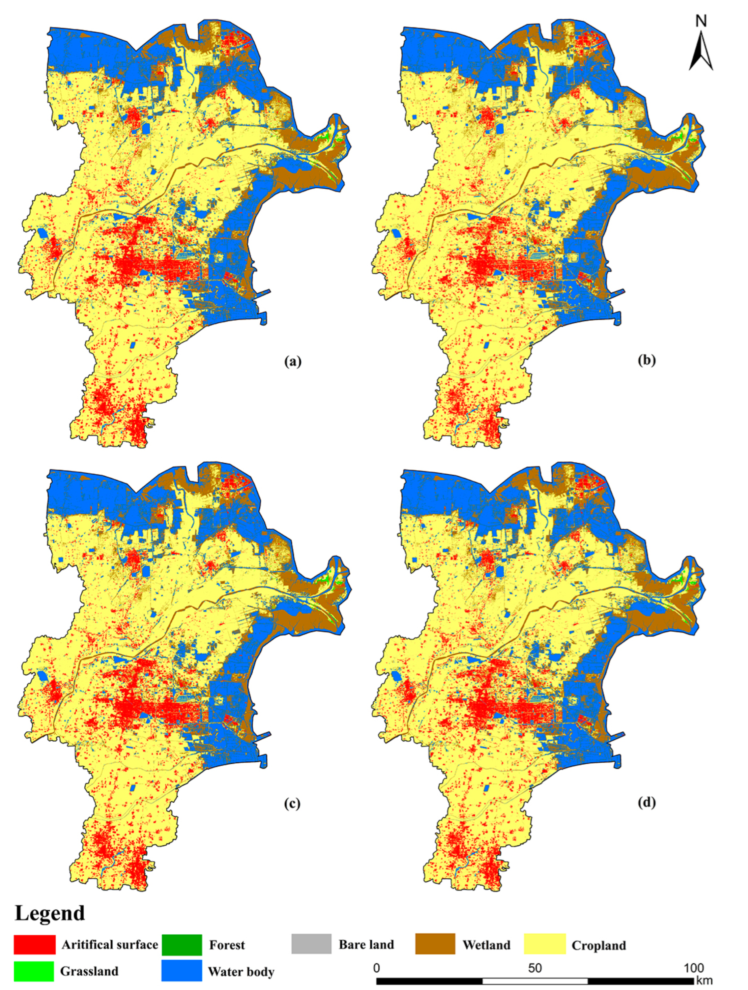
3.3. Multi-Scenario Land Use Simulation

The future projections showed that the cropland was still the largest LUT for YRD in 2030, followed by water body, wetland, and artificial surface. Most of the wetland and water body were distributed in the northern and eastern regions. Grassland, bare land, and forest combined account for less than 0.27% of the entire study region.
Regarding the temporal change in the LUCC in 2030 (Table A4), the wetland area increased significantly from 2020 to 2030 under the natural development (ND), urban construction and development (UCD), and ecological development (ED) scenarios, with an expansion of 4.10% for the ND scenario, 4.04% for the UCD scenario, and 4.28% for the ED scenario. In addition, the wetland area decreased by 0.3% under the cropland protection (CP) scenario at the same time. The results indicated that the cropland was the primary expansion source of wetland in this study area. The water body-changes trend was the same as for the wetland, and increased by 6.74% in the ND scenario, 6.71% in the UCD scenario, and 6.87% in the ED scenario; it also decreased by 0.65% in the CP scenario. Only in the CP scenario was the cropland area increased, growing by about 0.31%. The grassland and bare land decreased dramatically under all scenarios. In the context of the LUCC spatial change in 2030, the growth of the water body and wetland was mainly concentrated near the Yellow River estuary in the ND, UCD, and ED scenarios (Figure 6). The reduction in the cropland has caused the interface between cropland and wetland, as well as the water body shifting far away from the shoreline. The future expansion of the artificial surface was mainly concentrated in the central construction zone under the UCD scenario. The ED scenario was found to be the most suitable for regional development.

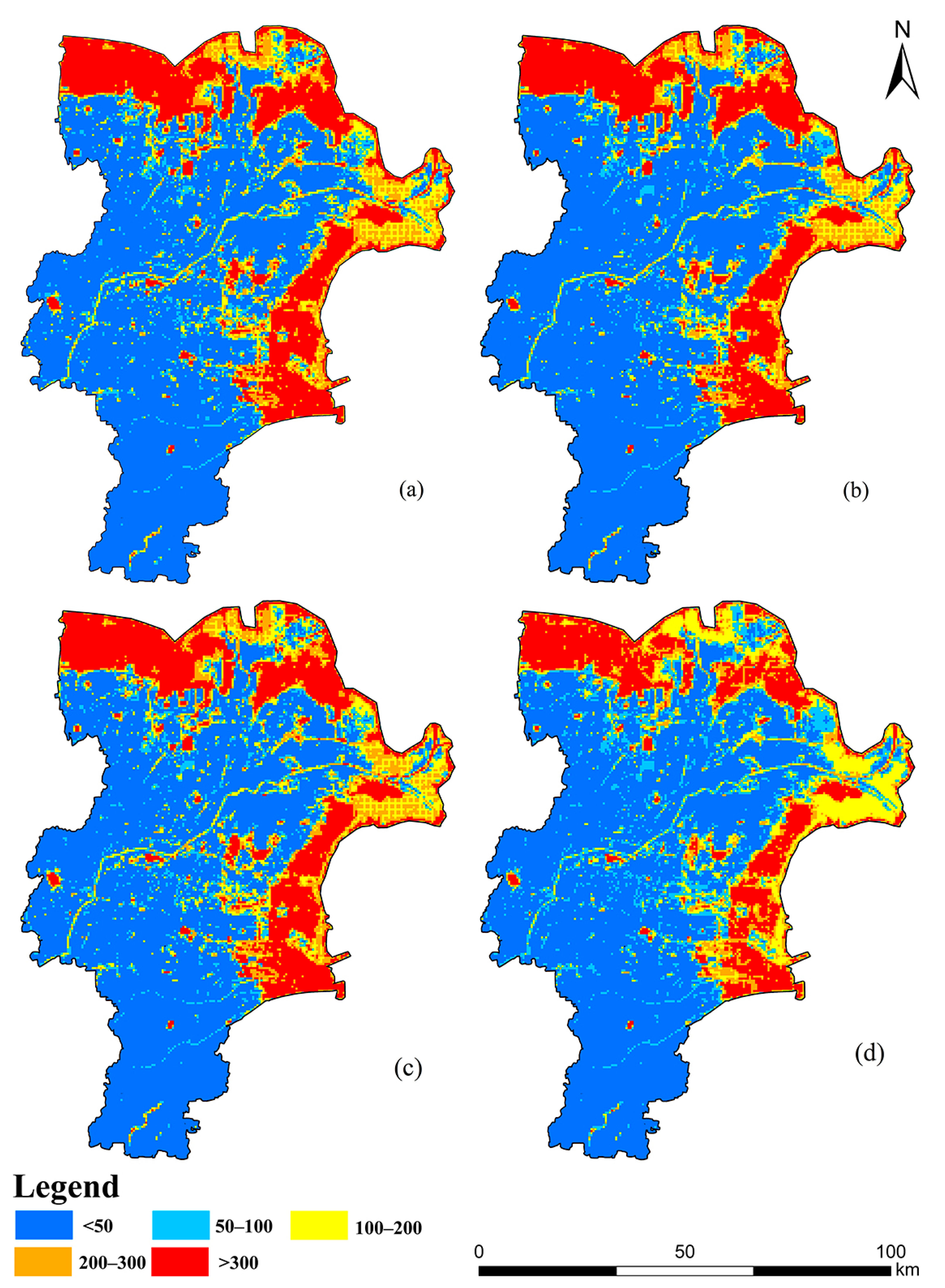
3.4. Characteristics of Changes in ESV under Multi-Scenarios

The total ESVs in 2030 in YRD under NP, UCD, CP, and ED scenarios were CNY 39.74 billion, CNY 37.56 billion, CNY 39.71 billion, and CNY 39.8 billion, respectively, with the change rate of 5.26%, 5.18%, −0.51%, and 5.42% compared with the total ESV in 2020, respectively. In the midst of them, the ND, UCD, and ED scenarios had a facilitating effect on the ESV improvement, and all of them had an increase of around 5%; correspondingly, the CP scenario showed a decrease in ESV by about −0.51% (Table A5).
In the ND scenario, the total ESV increased by CNY 1.98 billion from 2020 to 2030, primarily due to the conversion of cropland to water body and wetland. The decrease in ESV resulting from the conversion of cropland to artificial surface, water body, and wetland was a total of CNY 0.14 billion. In the CP scenario, the total ESV experienced a reduction of CNY 0.19 billion from 2020 to 2030, primarily due to restrictions on cropland transfer, leading to a decrease in water body and wetland areas. The cropland ESV experienced an increase of CNY 8.61 million, while the overall decrease in ESVs of water body and wetland amounted to CNY 0.2 billion. In the UCD scenario, the total ESV experienced an increase of CNY 1.96 billion, mainly due to the same reasons as in the ND scenario. Even though the expansion of the artificial surface caused a decrease in ESVs, it was much smaller in comparison to the increase brought by water body and wetland. In the ED scenario, the total ESV showed the largest growth, reaching a total of CNY 2.04 billion from 2000 to 2030, with the reason for the increase being the same as in the ND scenario. The ESVs of water body and wetland also recorded the largest increase in the ED scenario, with CNY 1.8 billion and CNY 0.38 billion, respectively. The ESV of the forest increased by 25% for the first time, while cropland and grassland exhibited the smallest ESV decrease, with −4.46% and 13.71%, respectively. In the ED scenario, not only wetlands were well protected and developed, but other land uses were also reasonably developed.
Figure 7 illustrates the distribution of the ESV across varying scenarios in 2030. With the exception of the CP scenario, the central area of the study region experienced a significant increase in the ESV range of CNY 0.5 to 1 million for other scenarios. The distribution of ESVs under the EP scenario exhibited a significant reduction, and the ESVs shifted from the range of CNY 2–3 million to the range of CNY 1–2 million. The ESV supplied by the water body on a per-area basis was significantly greater than that of the wetland, which predominantly explained this alteration. Additionally, the transformation of the water body into wetland led to an ESV decrease in particular regions of this area. These findings demonstrated that the advancement of diverse ecological service functions depended on a well-planned allocation of varying land use categories in the region.

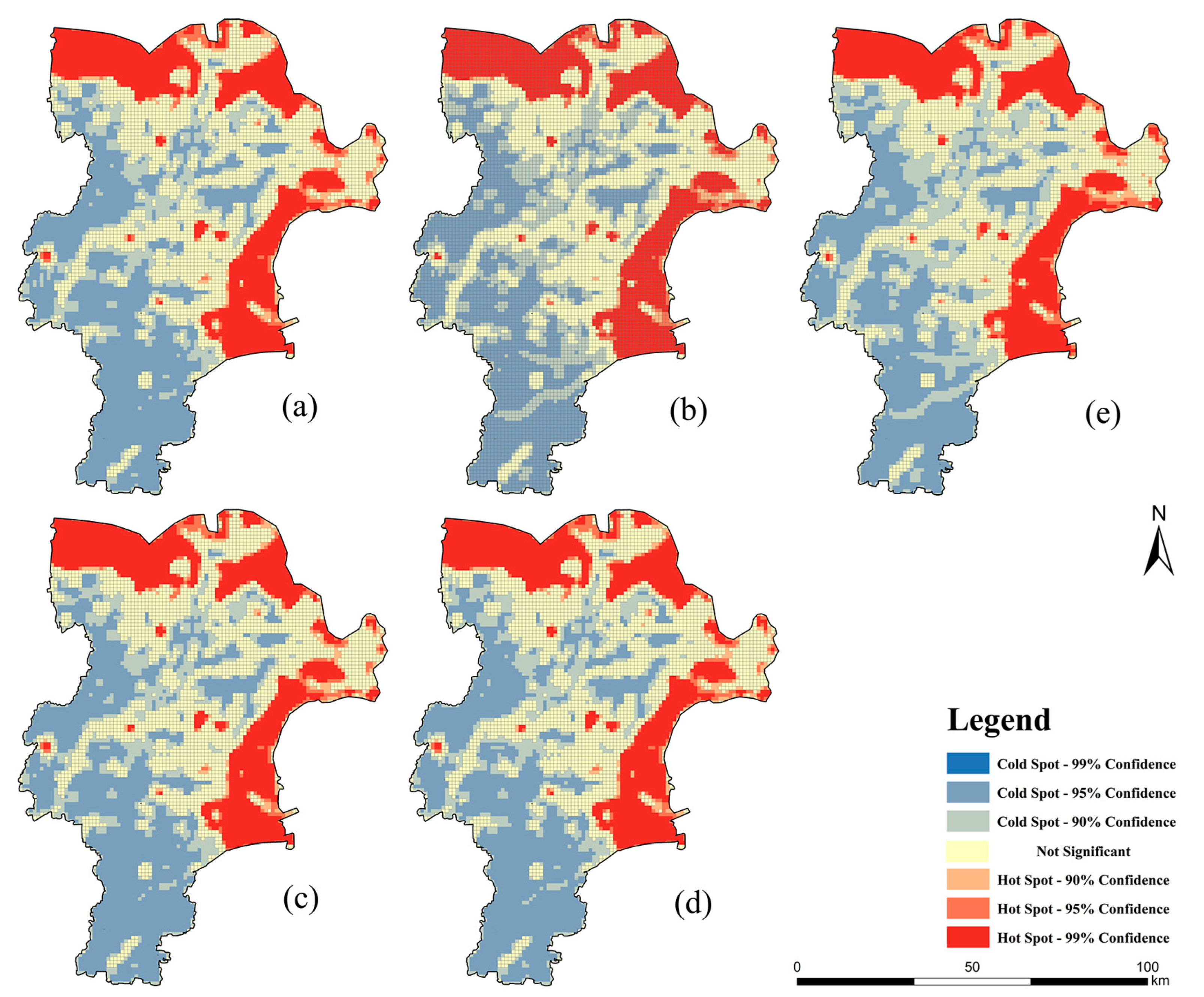
3.5. Hot Spot Assessment of ESV across Different Scenarios

To assess the ESV spatial clustering, the spatial statistical tool of ArcGIS was utilized to examine hot spots and cold spots within the study area. In 2020, ESV hot and cold spots were widespread and highly clustered, with hot spots predominantly located in the eastern and northern water body region, exhibiting a confidence level of nearly 99%. Meanwhile, the concentration of cold spots was in the southern region and western region. In comparison to 2020, the four scenarios that were modelled for 2030 were typically marked by a slight decrease in the range of hotspots’ distribution and a minor increase in cold spot regions (Figure 8).
Under the ND, UCD, and ED scenarios, a few small hot spots have emerged in the study region. The emergence of this phenomenon is the result of the increasing wetland area, which has led to a rise in ESV in this region. It was especially important to note that the 99% confidence level cold spots in the study region’s southern, western, and central sectors increased significantly under the UCD scenario, suggesting that the dispersion of artificial surface was mainly concentrated in this region, with a relatively minor impact on the wetland. The decrease in hot spots in the study region was caused by two factors: (1) the sources of wetland and water body have been in decline under the UCD scenario; and (2) some water bodies have been transformed into wetland, resulting in a decline in ESV and a weakening of aggregation.

4. Discussion

4.1. The Impact of Past and Future Trajectories of LUCC on ESVs in the YRD

During the study period, the wetland ESVs in the study area showed a decrease in total, consistent with the findings of previous research [55,56]. From an ESV contribution perspective, the water body was the highest contributor, followed by the wetland, together contributing nearly 90% of the ESV in the study region. Among them, the wetland alone accounts for over 22% of the ESVs. Wetland ecosystems can provide high ESVs [57] and serve several distinctive ecological functions, including ecological balance maintenance, biodiversity preservation, and water resource conservation [58]. The conversion of wetland to water body had increased regional ESVs. However, the wetland provided significantly higher ESVs than other LUTs in habitat and cultural services. The shift in wetland ESVs was closely related to wetland area changes [59]. In recent years, there was a fluctuation trend between the decrease and increase in the wetland area in YRD. The initial decrease in wetland area was primarily caused by the prolonged river cutoff time and expanded river cutoff range of the Yellow River, which resulted in a reduction in water flow from the river upstream. This resulted in wetland degradation [60]. In recent years, numerous wetland ecosystems, including intertidal zones, have been created due to the continuous expansion of aquaculture ponds and coastal salt production in the YRD. However, this has also resulted in a decline in the overall area of wetland ecosystems [61]. From the standpoint of land utilization transformation, cropland served as the principal source for the transfer in the wetland, and wetland predominantly transferred out to a water body. The amount of forest, grassland, and bare land within this study region was limited and had a relatively minor impact on alterations to the wetland. The artificial surface and wetland were spatially separated; thus, the artificial surface had a lower effect on the natural wetland environment.
In all simulation scenarios, the artificial surface increased at varying scales, which was in line with the findings of previous research [62]. The wetland area and ESVs decreased in the CP scenario due to the restricted alteration of cropland to other LUTs. In the ND, UCD, and ED scenarios, the wetland area exhibited a similar growth rate, and the increase in ESV showed a homogeneity in different scenarios. This provided additional evidence that the conversion of cropland in the study area significantly affected wetland. According to [63,64], a surge in population and economic growth has driven the rising need for artificial surfaces, further augmenting the expansion rate of the artificial surface in the UCD scenario. Under the ED scenario, the ecosystem was safeguarded and enhanced appropriately, leading to the greatest ESVs compared to other scenarios. This outcome was in line with the discoveries made by previous studies [65]. The distribution of ESV hot spots and cold spots revealed that a majority of ESV hot spots in the designated research zone were concentrated close to the water body. The distribution of hot spots in the wetland concentrated area was not pronounced, as the water body covered a larger area, and it can provide a higher ESV on a per-area basis compared to the wetland. However, when it comes to supply services and cultural services, wetlands played an irreplaceable role compared to other LUTs.

4.2. Policy Implications and Suggestions on YRD

Policy has a significant impact on land utilization. The results of the study showed that the area of aquaculture in YRD has expanded by 8.4 times in recent years [66], and the aquaculture area is mainly developed from wetland ecosystems such as mudflats, and the wetlands in the study area have been greatly damaged. It is important to note that policies such as ‘Opinions of Further Accelerating the Development of the Aquaculture Industry’ have played a significant role in this outcome. The implementation of policies such as the ‘National Wetland Conservation Action Plan’ has significantly mitigated the expansion of aquaculture in the study area, and some areas have begun to reduce aquaculture and restore wetlands that have been effectively protected and expanded [67].
Based on the obvious correlation between wetland ESV changes and other land utilization in the study area, wetland conservation policy in the future can be formulated in the following three aspects: (1) reduce the transfer of wetland to water bodies under the premise of securing water for domestic and production use; (2) since bare land can provide a negligible ESV per unit area, bare land will be selected for land utilization development instead of wetland, so as to reduce the degradation of wetland; and (3) aquaculture is a significant industry in the study area, occupying a large number of wetlands. To promote green development, it is necessary to implement relevant policies, transform the industry from high-speed to high-quality development, and reduce the number of aquaculture areas to restore wetland areas.

4.3. Limitations and Future Trends

The adjusted equivalence-coefficient method was used to estimate ESVs in YRD. Parameters such as grain production, the area of major grains, and the market price of major grains were selected to adjust the equivalence-coefficient method. Compared with other methods [68,69,70], this method requires fewer parameters and is easier to obtain. Therefore, it can calculate the ESV of global wetland ecosystems under the condition of limited data. However, this method is susceptible to inflation and the market economy [71]. The large fluctuations in market prices of major foodstuffs over a long time series lead to significant differences in the assessed ESVs of regions with similar land composition [72]. The accuracy and applicability of ESV assessments should be improved by incorporating various factors into the model.
The Markov–FLUS model can generate adaptive probabilities for different LUTs based on current land utilization data and six driving factors (DEM, road, temperature, precipitation, slope, and railways). It combines with an adaptive inertial competition mechanism to predict the distribution pattern of land utilization [73]. The unique mechanism can predict land use from both quantitative and spatial perspectives [74]. However, the accuracy of the model is affected by the combination of driving factors under different policies. For instance, the exclusion of ecosystem services in global policy frameworks is a reason for differences in wetland protection [75]. Additionally, the model’s accuracy decreases in regions other than the YRD due to varying driver choices under different policies. Outside the YRD region, the model’s accuracy decreased due to the use of different drivers resulting from policies. In the future, a global unified policy framework that combines multiple drivers could enhance the model’s predictive accuracy. This approach would be favorable for exploring the commonalities of wetland development across various regions.

5. Conclusions

This study calculated the ESV of major LUTs by combining the equivalent coefficients of ES after adjustments. The Markov–FLUS model was used to explore the changes in land utilization and ESV in the study area in 2030. The results indicate that wetland changes in the Yellow River Delta region were more frequent during the study period, with a trend of decrease followed by an increase. The ESV of wetland decreased by CNY 525 million. In total, 80.08% of the decrease in ESV in wetland was attributed to the conversion of wetlands into water body, while 69.1% of the increase in ESV in wetland was due to the conversion of cropland to wetland. The main LUTs affecting the change in wetland ESV in the study region were cropland and water body. The ED scenario was the most appropriate development mode for the wetland ecosystem. In the ND, UCD, and ED scenarios, the wetland area and ESV growth rate exceeded 4%. The wetland area and ESV exhibited a decline trend under the CP scenario, further suggesting that cropland is a major source of wetland transfer. This also suggests that the development of appropriate land policies is an effective means of achieving wetland conservation.

Author Contributions

Z.Z., L.H. and Z.F. crafted and orchestrated the research concepts; J.Z., S.W. and X.W. collected the data; Z.Z. and L.H. performed experiments and conducted analysis; Z.Z. prepared the original manuscript; L.H., Z.F. and J.F. reviewed and edited the manuscript. All authors have read and agreed to the published version of the manuscript.

Funding

This research was supported by the Guangdong Academy of Sciences to build a domestic first-class research institutions special fund project, grant number 2019GDASYL-0103003; by the Natural Science Foundation of Shandong Province, grant numbers ZR2020MD018 and ZR2020MD015; and by the National Natural Science Foundation of China, grant number 42171413.

Data Availability Statement

All data sources required for this article are listed in Section 2.2.

Conflicts of Interest

Author Jian Zhou was employed by the company Satellite (SHANDONG) Technology Group Co. The remaining authors declare that the research was conducted in the absence of any commercial or financial relationships that could be construed as a potential conflict of interest.

Appendix A

Some of the experimental data from the course of the study are presented in this appendix.
Figure A1. Land use distribution maps for the five time intervals in 2000–2020.
Sustainability 16 00619 g0a1
Table A1. Original ecosystem service equivalent factor.
FESSESCroplandForestGrasslandWater BodyWetlandArtificial SurfaceBare Land
Support servicesFood production0.850.23 0.23 0.80 0.5100.00
Raw material0.40.54 0.34 0.230.50 00
Water supply0.020.28 0.19 8.292.5900.00
Regulation servicesAir quality
regulation
0.671.76 1.21 0.771.90 00.02
Climate regulation0.365.27 3.19 2.293.60 00.00
Waste treatment0.11.57 1.05 5.553.60 00.10
Regulation of water flows0.273.81 2.34 102.2424.2300.03
Supply servicesErosion prevention1.032.14 1.47 0.932.3100.02
Maintenance of soil fertility0.120.16 0.11 0.070.1800.00
Habitat services0.131.95 1.34 2.557.8700.02
Cultural servicesCultural services0.060.86 0.59 1.894.7300.01
Table A2. Adjusted ecosystem service equivalent factor.
FESSESCroplandForestGrasslandWater BodyWetlandArtificial SurfaceBare Land
Support servicesFood production0.90 0.25 0.25 0.85 0.54 0.00 0.00
Raw material0.42 0.57 0.36 0.24 0.53 0.00 0.00
Water supply0.02 0.29 0.20 8.79 2.75 0.00 0.00
Regulation servicesAir quality
regulation
0.71 1.87 1.28 0.82 2.01 0.00 0.02
Climate regulation0.38 5.58 3.38 2.43 3.82 0.00 0.00
Waste treatment0.11 1.66 1.12 5.88 3.82 0.00 0.11
Regulation of water flows0.29 4.04 2.48 108.37 25.68 0.00 0.03
Supply servicesErosion prevention1.09 2.27 1.56 0.99 2.45 0.00 0.02
Maintenance of soil fertility0.13 0.17 0.12 0.07 0.19 0.00 0.00
Habitat services0.14 2.07 1.42 2.70 8.34 0.00 0.02
Cultural servicesCultural services0.06 0.91 0.63 2.00 5.01 0.00 0.01
Table A3. ES value (CNY/ha−1) for different land use types.
FESSESCroplandForestGrasslandWater BodyWetlandArtificial SurfaceBare Land
Support servicesFood production1284.22 352.53 352.53 1208.68 770.53 0.00 0.00
Raw material604.34 810.82 518.73 347.50 755.42 0.00 0.00
Water supply30.22 418.00 287.06 12,524.94 3913.10 0.00 0.00
Regulation servicesAir quality
regulation
1012.27 2659.10 1823.09 1163.35 2870.61 0.00 30.22
Climate regulation543.91 7957.14 4819.61 3459.85 5439.06 0.00 0.00
Waste treatment151.08 2367.00 1591.43 8385.22 5439.06 0.00 151.08
Regulation of water flows407.93 5756.34 3530.35 154,469.28 36,607.89 0.00 45.33
Supply servicesErosion prevention1556.18 3238.25 2220.95 1405.09 3490.06 0.00 30.22
Maintenance of soil fertility181.30 246.77 171.23 105.76 271.95 0.00 0.00
Habitat services196.41 2951.19 2019.50 3852.67 11,890.39 0.00 30.22
Cultural servicesCultural services90.65 1294.29 891.40 2855.51 7146.32 0.00 15.11
Table A4. Land use area in 2020 and multi-scenario.
Artificial SurfaceCroplandForestGrasslandBare LandWater BodyWetland
202061,447.37453,630.250.361899.45482.35138,029.81111,630.38
ND70,376.58431,099.460.271633.68462.33147,339.54116,204.67
CP61,578.27455,051.790.271598.22461.07137,130.12111,296.79
UCD72,782.28428,807.520.271631.16462.24147,288.51116,144.55
ED67,695.39433,402.830.451638.99460.71147,511.89116,406.27
Table A5. ESV (106 CNY) for different types of land use in different scenarios after simulation.
CroplandForestGrasslandWater BodyWetlandArtificial SurfaceBare LandTotal
20202748.320.0134.6226,195.008773.520.000.1537,751.62
ND2611.820.0129.7827,961.789133.040.000.1439,736.56
CP2756.930.0129.1326,024.268747.310.000.1437,557.77
UCD2597.930.0129.7327,952.109128.310.000.1439,708.22
ED2625.770.0129.8727,994.499148.880.000.1439,799.17

References

  1. Sannigrahi, S.; Bhatt, S.; Rahmat, S.; Paul, S.K.; Sen, S. Estimating global ecosystem service values and its response to land surface dynamics during 1995–2015. J. Environ. Manag. 2018, 223, 115–131. [Google Scholar] [CrossRef] [PubMed]
  2. Xu, D.; Ding, X. Assessing the impact of desertification dynamics on regional ecosystem service value in North China from 1981 to 2010. Ecosyst. Serv. 2018, 30, 172–180. [Google Scholar] [CrossRef]
  3. Ding, T.; Chen, J.; Fang, Z.; Wang, Y. Exploring the differences of ecosystem service values in different functional areas of metropolitan areas. Sustain. Prod. Consump. 2023, 38, 341–355. [Google Scholar] [CrossRef]
  4. Liu, Z.; Wu, R.; Chen, Y.; Fang, C.; Wang, S. Factors of ecosystem service values in a fast-developing region in China: Insights from the joint impacts of human activities and natural conditions. J. Clean. Prod. 2021, 297, 126588. [Google Scholar] [CrossRef]
  5. Fu, H.; Yan, Y. Ecosystem service value assessment in downtown for implementing the “Mountain-River-Forest-Cropland-Lake-Grassland system project”. Ecol. Indic. 2023, 154, 110751. [Google Scholar] [CrossRef]
  6. Peng, K.; Jiang, W.; Wang, X.; Hou, P.; Wu, Z.; Cui, T. Evaluation of future wetland changes under optimal scenarios and land degradation neutrality analysis in the Guangdong-Hong Kong-Macao Greater Bay Area. Sci. Total. Environ. 2023, 879, 163111. [Google Scholar] [CrossRef] [PubMed]
  7. Zhu, L.; Ke, Y.; Hong, J.; Zhang, Y.; Pan, Y. Assessing degradation of lake wetlands in Bashang Plateau, China based on long-term time series Landsat images using wetland degradation index. Ecol. Indic. 2022, 139, 108903. [Google Scholar] [CrossRef]
  8. Zhu, L.; Zhu, K.; Zeng, X. Evolution of landscape pattern and response of ecosystem service value in international wetland cities: A case study of Nanchang City. Ecol. Indic. 2023, 155, 110987. [Google Scholar] [CrossRef]
  9. Chen, K.; Cong, P.; Qu, L.; Liang, S.; Sun, Z. Wetland degradation diagnosis and zoning based on the integrated degradation index method. Ocean Coasta. Manag. 2022, 222, 106135. [Google Scholar] [CrossRef]
  10. Zhu, X.; Jiao, L.; Wu, X.; Du, D.; Wu, J.; Zhang, P. Ecosystem health assessment and comparison of natural and constructed wetlands in the arid zone of northwest China. Ecol. Indic. 2023, 154, 110576. [Google Scholar] [CrossRef]
  11. Anley, M.A.; Minale, A.S.; Haregeweyn, N.; Gashaw, T. Assessing the impacts of land use/cover changes on ecosystem service values in Rib watershed, Upper Blue Nile Basin, Ethiopia. Trees For. People 2022, 7, 100212. [Google Scholar] [CrossRef]
  12. Xin, X.; Zhang, T.; He, F.; Zhang, W.; Chen, K. Assessing and simulating changes in ecosystem service value based on land use/cover change in coastal cities: A case study of Shanghai, China. Ocean Coast. Manag. 2023, 239, 106591. [Google Scholar] [CrossRef]
  13. Yin, Z.; Feng, Q.; Zhu, R.; Wang, L.; Chen, Z.; Fang, C.; Lu, R. Analysis and prediction of the impact of land use/cover change on ecosystem services value in Gansu province, China. Ecol. Indic. 2023, 154, 110868. [Google Scholar] [CrossRef]
  14. Rawat, L.S.; Maikhuri, R.K.; Bahuguna, Y.M.; Jugran, A.K.; Maletha, A.; Jha, N.K.; Phondani, P.C.; Dhyani, D.; Pharswan, D.S.; Chamoli, S. Rejuvenating ecosystem services through reclaiming degraded land for sustainable societal development: Implications for conservation and human wellbeing. Land Use Policy 2022, 112, 105804. [Google Scholar] [CrossRef]
  15. Cai, G.; Xiong, J.; Wen, L.; Weng, A.; Lin, Y.; Li, B. Predicting the ecosystem service values and constructing ecological security patterns in future changing land use patterns. Ecol. Indic. 2023, 154, 110787. [Google Scholar] [CrossRef]
  16. Cao, Y.; Kong, L.; Zhang, L.; Ouyang, Z. The balance between economic development and ecosystem service value in the process of land urbanization: A case study of China’s land urbanization from 2000 to 2015. Land Use Policy 2021, 108, 105536. [Google Scholar] [CrossRef]
  17. Rotich, B.; Kindu, M.; Kipkulei, H.; Kibet, S.; Ojwang, D. Impact of land use/land cover changes on ecosystem service values in the cherangany hills water tower, Kenya. Environ. Chall. 2022, 8, 100576. [Google Scholar] [CrossRef]
  18. Wei, F.; Xiang, M.; Deng, L.; Wang, Y.; Li, W.; Yang, S.; Wu, Z. Spatiotemporal Distribution Characteristics and Their Driving Forces of Ecological Service Value in Transitional Geospace: A Case Study in the Upper Reaches of the Minjiang River, China. Sustainability 2023, 15, 14559. [Google Scholar] [CrossRef]
  19. Zhou, Y.; Chen, T.; Wang, J.; Xu, X. Analyzing the Factors Driving the Changes of Ecosystem Service Value in the Liangzi Lake Basin—A GeoDetector-Based Application. Sustainability 2023, 15, 15763. [Google Scholar] [CrossRef]
  20. Jiang, W.; Lü, Y.; Liu, Y.; Gao, W. Ecosystem service value of the Qinghai-Tibet Plateau significantly increased during 25 years. Ecosyst. Serv. 2020, 44, 101146. [Google Scholar] [CrossRef]
  21. Admasu, S.; Yeshitela, K.; Argaw, M. Impact of land use land cover changes on ecosystem service values in the Dire and Legedadi watersheds, central highlands of Ethiopia: Implication for landscape management decision making. Heliyon 2023, 9, e15352. [Google Scholar] [CrossRef] [PubMed]
  22. Molinero-Parejo, R.; Aguilera-Benavente, F.; Gómez-Delgado, M.; Shurupov, N. Combining a land parcel cellular automata (LP-CA) model with participatory approaches in the simulation of disruptive future scenarios of urban land use change. Comput. Environ. Urban 2023, 99, 101895. [Google Scholar] [CrossRef]
  23. Aniah, P.; Bawakyillenuo, S.; Codjoe, S.; Dzanku, F. Land use and land cover change detection and prediction based on CA-Markov chain in the savannah ecological zone of Ghana. Environ. Chall. 2023, 10, 100664. [Google Scholar] [CrossRef]
  24. Lin, W.; Sun, Y.; Nijhuis, S.; Wang, Z. Scenario-based flood risk assessment for urbanizing deltas using future land-use simulation (FLUS): Guangzhou Metropolitan Area as a case study. Sci. Total. Environ. 2020, 739, 139899. [Google Scholar] [CrossRef] [PubMed]
  25. Girma, R.; Fürst, C.; Moges, A. Land use land cover change modeling by integrating artificial neural network with cellular Automata-Markov chain model in Gidabo river basin, main Ethiopian rift. Environ. Chall. 2022, 6, 100419. [Google Scholar] [CrossRef]
  26. Ma, B.; Wang, X. What is the future of ecological space in Wuhan Metropolitan Area? A multi-scenario simulation based on Markov-FLUS. Ecol. Indic. 2022, 141, 109124. [Google Scholar] [CrossRef]
  27. Qiu, J.; Huang, T.; Yu, D. Evaluation and optimization of ecosystem services under different land use scenarios in a semiarid landscape mosaic. Ecol. Indic. 2022, 135, 108516. [Google Scholar] [CrossRef]
  28. Xie, G.; Zhang, C.; Zhen, L.; Zhang, L. Dynamic changes in the value of China’s ecosystem services. Ecosyst. Serv. 2017, 26, 146–154. [Google Scholar] [CrossRef]
  29. Lusardi, J.; Sunderland, T.J.; Crowe, A.; Jackson, B.M.; Jones, G. Can process-based modelling and economic valuation of ecosystem services inform land management policy at a catchment scale? Land Use Policy 2020, 96, 104636. [Google Scholar] [CrossRef]
  30. Pan, D.; Yan, H.; Han, T.; Sun, B.; Jiang, J.; Liu, X.; Li, X.; Wang, H. Evaluation of the service function value of grassland ecosystems in Gansu Province using the equivalence factor method. Pratacultural Sci. 2021, 338, 1860–1868. [Google Scholar]
  31. Su, K.; Wei, D.; Lin, W. Evaluation of ecosystem services value and its implications for policy making in China—A case study of Fujian province. Ecol. Indic. 2020, 108, 105752. [Google Scholar] [CrossRef]
  32. Wu, K.; Wang, D.; Lu, H.; Liu, G. Temporal and spatial heterogeneity of land use, urbanization, and ecosystem service value in China: A national-scale analysis. J. Clean. Prod. 2023, 418, 137911. [Google Scholar] [CrossRef]
  33. Yang, Y.; Wang, K.; Liu, D.; Zhao, X.; Fan, J. Effects of land-use conversions on the ecosystem services in the agro-pastoral ecotone of northern China. J. Clean. Prod. 2020, 249, 119360. [Google Scholar] [CrossRef]
  34. Zhao, Q.; Wen, Z.; Chen, S.; Ding, S.; Zhang, M. Quantifying Land Use/Land Cover and Landscape Pattern Changes and Impacts on Ecosystem Services. Int. J. Environ. Res. Public Health 2020, 17, 126. [Google Scholar] [CrossRef] [PubMed]
  35. Hu, Z.; Gong, J.; Li, J.; Li, R.; Zhang, Z.; Zhong, F.; Wen, C. Valuing the coordinated development of urbanization and ecosystem service value in border counties. J. Clean. Prod. 2023, 415, 137799. [Google Scholar] [CrossRef]
  36. Tan, Z.; Guan, Q.; Lin, J.; Yang, L.; Luo, H.; Ma, Y.; Tian, J.; Wang, Q.; Wang, N. The response and simulation of ecosystem services value to land use/land cover in an oasis, Northwest China. Ecol. Indic. 2020, 118, 106711. [Google Scholar] [CrossRef]
  37. Zhang, X.; Zheng, Z.; Sun, S.; Wen, Y.; Chen, H. Study on the driving factors of ecosystem service value under the dual influence of natural environment and human activities. J. Clean. Prod. 2023, 420, 138408. [Google Scholar] [CrossRef]
  38. Wang, C.; Wang, Y.; Wang, R.; Zheng, P. Modeling and evaluating land-use/land-cover change for urban planning and sustainability: A case study of Dongying city, China. J. Clean. Prod. 2018, 172, 1529–1534. [Google Scholar] [CrossRef]
  39. Zheng, X.; Javed, Z.; Liu, C.; Tanvir, A.; Sandhu, O.; Liu, H.; Ji, X.; Xing, C.; Lin, H.; Du, D. MAX-DOAS and in-situ measurements of aerosols and trace gases over Dongying, China: Insight into ozone formation sensitivity based on secondary HCHO. J. Environ. Sci. 2024, 135, 656–668. [Google Scholar] [CrossRef]
  40. Zhang, T.; Zhang, S.; Cao, Q.; Wang, H.; Li, Y. The spatiotemporal dynamics of ecosystem services bundles and the social-economic-ecological drivers in the Yellow River Delta region. Ecol. Indic. 2022, 135, 108573. [Google Scholar] [CrossRef]
  41. Madrigal-Martínez, S.; Puga-Calderón, R.J.; Castromonte-Miranda, J.; Cáceres, V.A. Mapping the benefits and the exchange values of provisioning ecosystem services using GIS and local ecological knowledge in a high-Andean community. Remote Sens. Appl. 2023, 30, 100971. [Google Scholar] [CrossRef]
  42. Zhang, X.; Liu, L.; Chen, X.; Gao, Y.; Xie, S.; Mi, J. GLC_FCS30: Global land-cover product with fine classification system at 30 m using time-series Landsat imagery. Earth Syst. Sci. Data 2021, 13, 2753–2776. [Google Scholar] [CrossRef]
  43. Redo, D.J.; Aide, T.; Clark, M.L.; Andrade-Núnez, M. Impacts of internal and external policies on land change in Uruguay, 2001–2009. Environ. Conserv. 2012, 39, 122–131. [Google Scholar] [CrossRef]
  44. He, N.; Zhou, Y.; Wang, L.; Li, Q.; Zuo, Q.; Liu, J. Spatiotemporal differentiation and the coupling analysis of ecosystem service value with land use change in Hubei Province, China. Ecol. Indic. 2022, 145, 109693. [Google Scholar] [CrossRef]
  45. Sun, X.; Li, S.; Zhai, X.; Wei, X.; Yan, C. Ecosystem changes revealed by land cover in the Three-River Headwaters Region of Qinghai, China (1990–2015). Res. Cold Arid Reg. 2023, 15, 85–91. [Google Scholar] [CrossRef]
  46. Belay, T.; Melese, T.; Senamaw, A. Impacts of land use and land cover change on ecosystem service values in the Afroalpine area of Guna Mountain, Northwest Ethiopia. Heliyon 2022, 8, e12246. [Google Scholar] [CrossRef]
  47. Pham, K.T.; Lin, T.H. Effects of urbanisation on ecosystem service values: A case study of Nha Trang, Vietnam. Land Use Policy 2023, 128, 106599. [Google Scholar] [CrossRef]
  48. Yu, Q.; Feng, C.; Shi, Y.; Guo, L. Spatiotemporal interaction between ecosystem services and urbanization in China: Incorporating the scarcity effects. J. Clean. Prod. 2021, 317, 128392. [Google Scholar] [CrossRef]
  49. Xie, G.; Zhang, C.; Zhang, L.; Chen, W.; Li, S. Improvement of the Evaluation Method for Ecosystem Service Value Based on Per Unit Area. J. Nat. Resour. 2015, 30, 1243–1254. [Google Scholar]
  50. Berhanu, Y.; Dalle, G.; Sintayehu, D.W.; Kelboro, G.; Nigussie, A. Land use/land cover dynamics driven changes in woody species diversity and ecosystem services value in tropical rainforest frontier: A 20-year history. Heliyon 2023, 9, e13711. [Google Scholar] [CrossRef]
  51. Asori, M.; Adu, P. Modeling the impact of the future state of land use land cover change patterns on land surface temperatures beyond the frontiers of greater Kumasi: A coupled cellular automaton (CA) and Markov chains approaches. Remote Sens. Appl. 2023, 29, 100908. [Google Scholar] [CrossRef]
  52. Liu, P.; Hu, Y.; Jia, W. Land use optimization research based on FLUS model and ecosystem services–setting Jinan City as an example. Urban Clim. 2021, 40, 100984. [Google Scholar] [CrossRef]
  53. Chowdhury, M. Comparison of Accuracy and Reliability of Random Forest, Support Vector Machine, Artificial Neural Network and Maximum Likelihood method in Land use/cover Classification of Urban Setting. Environ. Chall. 2023, 14, 100800. [Google Scholar] [CrossRef]
  54. Xiao, Y.; Huang, M.; Xie, G.; Zhen, L. Evaluating the impacts of land use change on ecosystem service values under multiple scenarios in the Hunshandake region of China. Sci. Total Environ. 2022, 850, 158067. [Google Scholar] [CrossRef]
  55. Abera, W.; Tamene, L.; Kassawmar, T.; Mulatu, K.; Kassa, H.; Verchot, L.; Quintero, M. Impacts of land use and land cover dynamics on ecosystem services in the Yayo coffee forest biosphere reserve, southwestern Ethiopia. Ecosyst. Serv. 2021, 50, 101338. [Google Scholar] [CrossRef]
  56. Abd El-Hamid, H.T.; Toubar, M.M.; Zarzoura, F.; El-Alfy, M.A. Ecosystem services based on land use/cover and socio-economic factors in Lake Burullus, a Ramsar Site, Egypt. Remote Sens. Appl. 2023, 30, 100979. [Google Scholar] [CrossRef]
  57. Tolessa, T.; Kidane, M.; Bezie, A. Assessment of the linkages between ecosystem service provision and land use/land cover change in Fincha watershed, North-Western Ethiopia. Heliyon 2021, 7, e07673. [Google Scholar] [CrossRef] [PubMed]
  58. Xu, Y.; Xie, Y.; Wu, X.; Xie, Y.; Zhang, T.; Zou, Z.; Zhang, R.; Zhang, Z. Evaluating temporal-spatial variations of wetland ecosystem service value in China during 1990–2020 from the donor side based on cosmic exergy. J. Clean. Prod. 2023, 414, 137485. [Google Scholar] [CrossRef]
  59. Cai, Y.; Zhang, P.; Wang, Q.; Wu, Y.; Ding, Y.; Nabi, M.; Fu, C.; Wang, H.; Wang, Q. How does water diversion affect land use change and ecosystem service: A case study of Baiyangdian wetland, China. J. Environ. Manag. 2023, 344, 118558. [Google Scholar] [CrossRef]
  60. Sun, Z.; Mou, X.; Chen, X.; Wang, L.; Song, H. Actualities, problems and suggestions of wetland protection and restoration in the Yellow River Delta. Wetl. Sci. 2011, 9, 107–115. [Google Scholar]
  61. Fan, Y.; Chen, S.; Zhao, B.; Yu, S.; Ji, H.; Jiang, C. Monitoring tidal flat dynamics affected by human activities along an eroded coast in the Yellow River Delta, China. Environ. Monit. Assess. 2018, 190, 396. [Google Scholar] [CrossRef] [PubMed]
  62. Shi, Q.; Gu, C.; Xiao, C. Multiple scenarios analysis on land use simulation by coupling socioeconomic and ecological sustainability in Shanghai, China. Sustain. Cities Soc. 2023, 95, 104578. [Google Scholar] [CrossRef]
  63. Cao, Y. Forces driving changes in urban construction land of urban agglomerations in China. J. Urban Plan Dasce. 2015, 141, 05014011. [Google Scholar] [CrossRef]
  64. Sheng, X.; Cao, Y.; Zhou, W.; Zhang, H.; Song, L. Multiple scenario simulations of land use changes and countermeasures for collaborative development mode in Chaobai River region of Jing-Jin-Ji, China. Habitat Int. 2018, 82, 38–47. [Google Scholar] [CrossRef]
  65. Zhang, Y.; Yu, P.; Tian, Y.; Chen, H.; Chen, Y. Exploring the impact of integrated spatial function zones on land use dynamics and ecosystem services tradeoffs based on a future land use simulation (FLUS) model. Ecol. Indic. 2023, 150, 110246. [Google Scholar] [CrossRef]
  66. Yan, J.; Zhu, J.; Zhao, S.; Su, F. Coastal wetland degradation and ecosystem service value change in the Yellow River Delta, China. Glob. Ecol. Conserv. 2023, 44, e02501. [Google Scholar] [CrossRef]
  67. Long, X.; Lin, H.; An, X.; Chen, S.; Qi, S.; Zhang, M. Evaluation and analysis of ecosystem service value based on land use/cover change in Dongting Lake wetland. Ecol. Indic. 2022, 136, 108619. [Google Scholar] [CrossRef]
  68. Zeng, Q.; Ye, X.; Cao, Y.; Chuai, X.; Xu, H. Impact of expanded built-up land on ecosystem service value by considering regional interactions. Ecol. Indic. 2023, 153, 110397. [Google Scholar] [CrossRef]
  69. Zhai, Y.; Li, W.; Shi, S.; Gao, Y.; Chen, Y.; Ding, Y. Spatio-temporal dynamics of ecosystem service values in China’s Northeast Tiger-Leopard National Park from 2005 to 2020: Evidence from environmental factors and land use/land cover changes. Ecol. Indic. 2023, 155, 110734. [Google Scholar] [CrossRef]
  70. Wang, Y.; Zhang, Z.; Chen, X. Spatiotemporal change in ecosystem service value in response to land use change in Guizhou Province, southwest China. Ecol. Indic. 2022, 144, 109514. [Google Scholar] [CrossRef]
  71. Sun, X.; Li, Y.; Zhu, X.; Cao, K.; Feng, L. Integrative assessment and management implications on ecosystem services loss of coastal wetlands due to reclamation. J. Clean Prod. 2017, 163, S101–S112. [Google Scholar] [CrossRef]
  72. Pan, N.; Guan, Q.; Wang, Q.; Sun, Y.; Li, H.; Ma, Y. Spatial Differentiation and Driving Mechanisms in Ecosystem Service Value of Arid Region: A case study in the middle and lower reaches of Shule River Basin, NW China. J. Clean Prod. 2021, 319, 128718. [Google Scholar] [CrossRef]
  73. Xiang, S.; Wang, Y.; Deng, H.; Yang, C.; Wang, Z.; Gao, M. Response and multi-scenario prediction of carbon storage to land use/cover change in the main urban area of Chongqing, China. Ecol. Indic. 2022, 142, 109205. [Google Scholar] [CrossRef]
  74. Wang, Q.; Guan, Q.; Lin, J.; Luo, H.; Tan, Z.; Ma, Y. Simulating land use/land cover change in an arid region with the coupling models. Ecol. Indic. 2021, 122, 107231. [Google Scholar] [CrossRef]
  75. Bell-James, J.; Foster, R.; Lovelock, C.E. Identifying priorities for reform to integrate coastal wetland ecosystem services into law and policy. Environ. Sci. Policy 2023, 142, 164–172. [Google Scholar] [CrossRef]
Figure 1. The study area of YRD.
Sustainability 16 00619 g001
Figure 2. Single extent dynamic of land utilization during the periods of 2000–2005, 2005–2010, 2010–2015, and 2015–2020.
Sustainability 16 00619 g002
Figure 3. Chord diagrams of LUCC conversion during 2000–2005 (a), 2005–2010 (b), 2010–2015 (c), 2015–2020 (d), and 2000–2020 (e).
Sustainability 16 00619 g003
Figure 4. The ESVs of FES and SES in YRD from 2000 to 2020.
Sustainability 16 00619 g004
Figure 5. The ESV spatial–temporal changes in YRD from 2000 to 2020 (CNY ten thousand).
Sustainability 16 00619 g005
Figure 6. Simulation of LUCC in YRD in 2030 under ND scenario (a), CP scenario (b), UCD scenario (c), and ED scenario (d).
Sustainability 16 00619 g006
Figure 7. ESV changes under ND scenario (a), CP scenario (b), UCD scenario (c), and ED scenario (d).
Sustainability 16 00619 g007
Figure 8. Prediction of ESV hot spots and cold spots in YRD region in 2030 under ND scenario (a), CP scenario (b), UCD scenario (c), and ED scenario (d). The result of 2020 (e).
Sustainability 16 00619 g008
Table 1. Area and scale of different land use types in 2000, 2005, 2010, 2015, and 2020.
20002005201020152020
Area
/ha
Proportion/%Area
/ha
Proportion/%Area
/ha
Proportion/%Area
/ha
Proportion/%Area
/ha
Proportion/%
Artificial surface39,649.275.1747,000.026.1352,139.226.8059,369.237.7461,447.378.01
Cropland504,680.1465.79487,304.2363.52478,055.5962.32465,109.3060.63453,630.2559.13
Forest79.260.0168.190.0148.220.0141.260.010.360.00
Grassland2817.720.372808.930.372383.190.312251.590.291899.450.25
Bare land250.710.03298.070.04343.990.04394.370.05482.350.06
Water body101,338.4613.21121,427.6915.83127,864.8116.67134,012.8717.47138,029.8117.99
Wetland118,310.2815.42108,216.6414.11106,287.8113.86105,941.7813.81111,630.3814.55
Table 2. The ESV of the study area from 2000 to 2020.
CroplandForestGrasslandWater BodyWetlandArtificial SurfaceBare LandTotal
2000ESV/109 CNY 3.060.002200.05119.239.300.000.0000831.64
Proportion/% 9.660.010000.16060.7829.390.000.00024100.00
2005ESV/109 CNY2.950.001900.05123.048.510.000.0000934.56
Proportion/% 8.540.010000.15066.6924.610.000.00026100.00
2010ESV/109 CNY2.900.001400.04324.278.350.000.0001035.56
Proportion/% 8.140.004000.12068.2423.490.000.00029100.00
2015ESV/109 CNY 2.810.001200.04125.438.330.000.0001236.62
Proportion/% 7.700.003000.11069.4522.740.000.00033100.00
2020ESV/109 CNY2.740.000010.03526.198.770.000.0001537.75
Proportion/% 7.280.000030.09069.3923.240.000.00039100.00
Disclaimer/Publisher’s Note: The statements, opinions and data contained in all publications are solely those of the individual author(s) and contributor(s) and not of MDPI and/or the editor(s). MDPI and/or the editor(s) disclaim responsibility for any injury to people or property resulting from any ideas, methods, instructions or products referred to in the content.

