


Assessing Polarisation of Climate Phenomena Based on Long-Term Precipitation and Temperature Sequences


Abstract
1. Introduction
2. Interactions between Polarisation and Sustainable Development
- Degradation of natural resources: extreme phenomena such as droughts and floods can accelerate the degradation of natural resources, threatening ecological balance and future generations [77];
- Social inequality: the poorest communities, with limited capacity to adapt to climate change, are the most vulnerable to its negative effects, potentially deepening social inequalities [78];
- Challenges to infrastructure and industry: extreme weather events can disrupt the functioning of infrastructure and industry, leading to economic destabilisation [50];
- Increased environmental awareness: climate polarisation can lead to greater social awareness of climate change, fostering more sustainable actions [82];
- Increased efficiency and resilience of systems: communities and industries may strive for greater efficiency in resource use, reducing waste and supporting sustainable management [55];
- Strengthening global cooperation: shared climate challenges may lead to closer international cooperation in support of sustainable development [85].
3. Preparation of Data for Analysis
4. The Polarisation of Precipitation and Temperature Phenomena
- Changes in atmospheric circulation: fluctuations in atmospheric circulation, such as changes in belt and monsoon patterns, can concentrate precipitation in certain regions, while other areas experience precipitation deficits [95];
- El Niño and La Niña phenomena: these can lead to abrupt changes in ocean surface temperature, which affects rainfall patterns; areas that are normally wet can experience drought during El Niño, and dry areas can become flooded during La Niña [46];
- Topographical changes: high mountain ranges can affect the movement of air masses and cloud formation, leading to more rainfall on one side of the mountain and droughts on the other [46];
- Urbanisation and land use changes: urban growth and land use changes can alter the microclimate and affect the distribution of precipitation in an area [46].
- Changes in atmospheric circulation: may bring higher temperatures to tropical areas, while areas under the influence of lows may experience cooling [95];
- Changes in greenhouse gases: increases in greenhouse gas concentrations can lead to an overall warming of the climate, but some areas may experience faster temperature increases than others [72];
- Impact of urban areas: cities create so-called “heat islands” where concrete and asphalt absorb and retain heat, which can lead to significant heating of urban areas [97].
- Increased weather variability: polarisation of precipitation can lead to abrupt and unpredictable changes in weather patterns, which can make planning for agricultural and infrastructure activities difficult [36];
- Risk of natural disasters: extremes of rainfall can increase the risk of natural disasters, such as floods in areas of increased rainfall or droughts in areas of decreased rainfall [60];
- Impact on water availability: precipitation polarisation can lead to reduced water availability in drought-affected areas and increased risk of soil erosion during periods of intense rainfall [98];
- Impact on ecosystems: extreme precipitation conditions can affect ecosystem structures and services, with potential implications for biodiversity and ecosystem products [84].
- Human health risks: temperature extremes, both heat and cold, can pose a risk to human health, leading to heat- or cold-related diseases [60];
- Effects on agriculture and food production: extreme temperatures can affect plant growth processes, leading to reduced yields and loss of quality in agricultural products [80];
- Changes in species distribution: extreme temperatures can affect the distribution areas of different animal and plant species, which can disrupt the balance of ecosystems [99];
- Changes in water levels: glacial melting and ocean warming associated with temperature polarisation can lead to rising sea and ocean levels [100].
- Increased risk of natural disasters: the combination of extreme rainfall and temperatures can amplify the risk of floods, landslides, and other natural disasters [76];
- Impact on agri-food production: extreme precipitation and temperatures can negatively affect food production, which can lead to food security problems [60];
- Changes in the landscape: the interaction of extreme rainfall and temperatures can lead to changes in the landscape, such as soil erosion and degradation of natural areas [60].
5. The Concept of Polarisation Measure
- The concentration ratio [110] determines the degree of concentration of values at one end of the distribution and is similar to the Gini coefficient. However, it should be noted that the Gini coefficient may be less useful in analysing asymmetric distributions, which means that other indicators such as the concentration ratio or Lorenz curve should be considered in such cases.
- The GMD (Gini mean difference) index [111] is an inequality measure used in statistical and econometric analysis to measure polarisation or inequality in a sample distribution. Unlike the Gini coefficient, which measures unevenness, the GMD index enables the analysis of unevenness in the distribution of any variable, such as income, age, weight, height, precipitation, or temperature. The GMD index ranges from zero to one, where zero indicates complete evenness in the distribution and one indicates the concentration of all values in one class. The higher the GMD index value, the greater the unevenness in the variable distribution.
- The Lorenz indicator [105,108] is an inequality indicator in a distribution, which is based on the Lorenz curve. It is often used to measure income inequality but can also be used to measure inequality in other quantitative variables, including climate change studies. Higher values of the Lorenz curve indicate greater inequality in the occurrence of climate change effects such as droughts, floods, or sea level rises, meaning that some regions or social groups are more vulnerable to the effects of climate change than others.
- The Atkinson index [104] is a measure of inequality in the distribution of quantitative variables, which is based on the idea of absolute deviations. It takes into account the differences between groups of values in the distribution; it is similar to the Gini index, but focuses more on average values than extreme values.
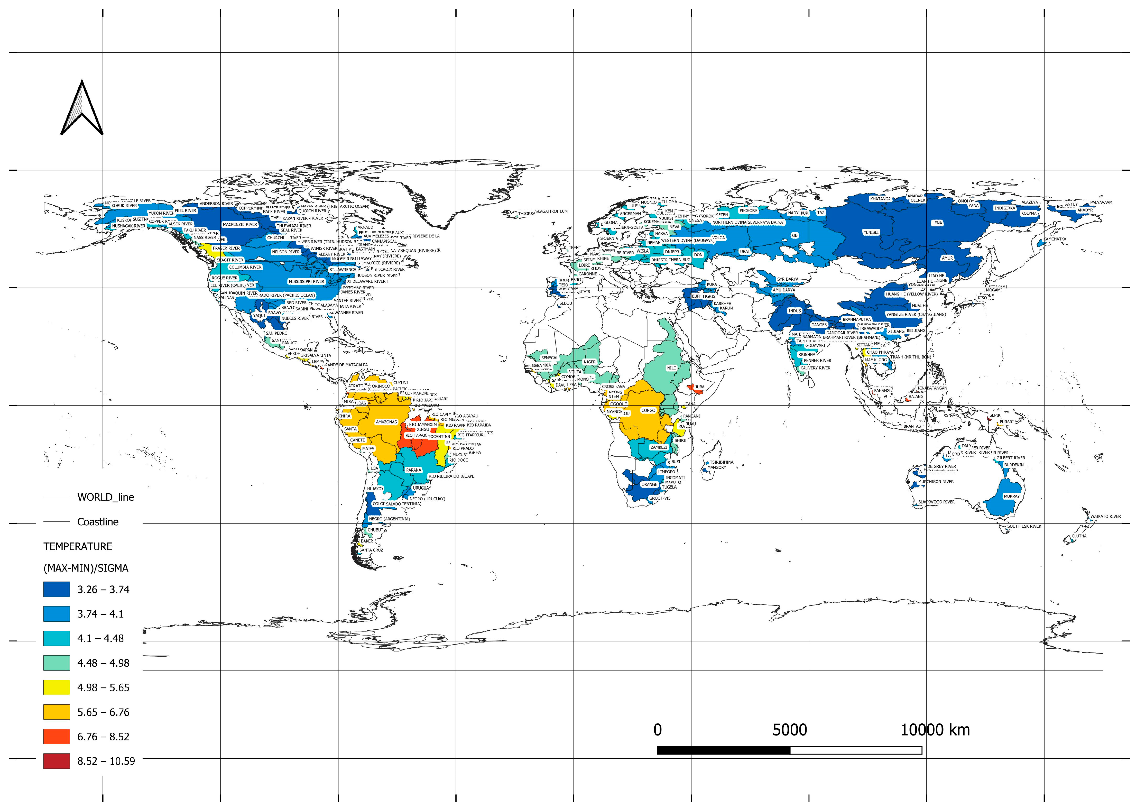
- Range relates to values calculated as max–min usually referring to the difference between the maximum and minimum values of a given variable in a specific period of time. In the case of assessing the polarisation of precipitation and temperature, max–min can be used as a measure of the amplitude of these variables in a given period.
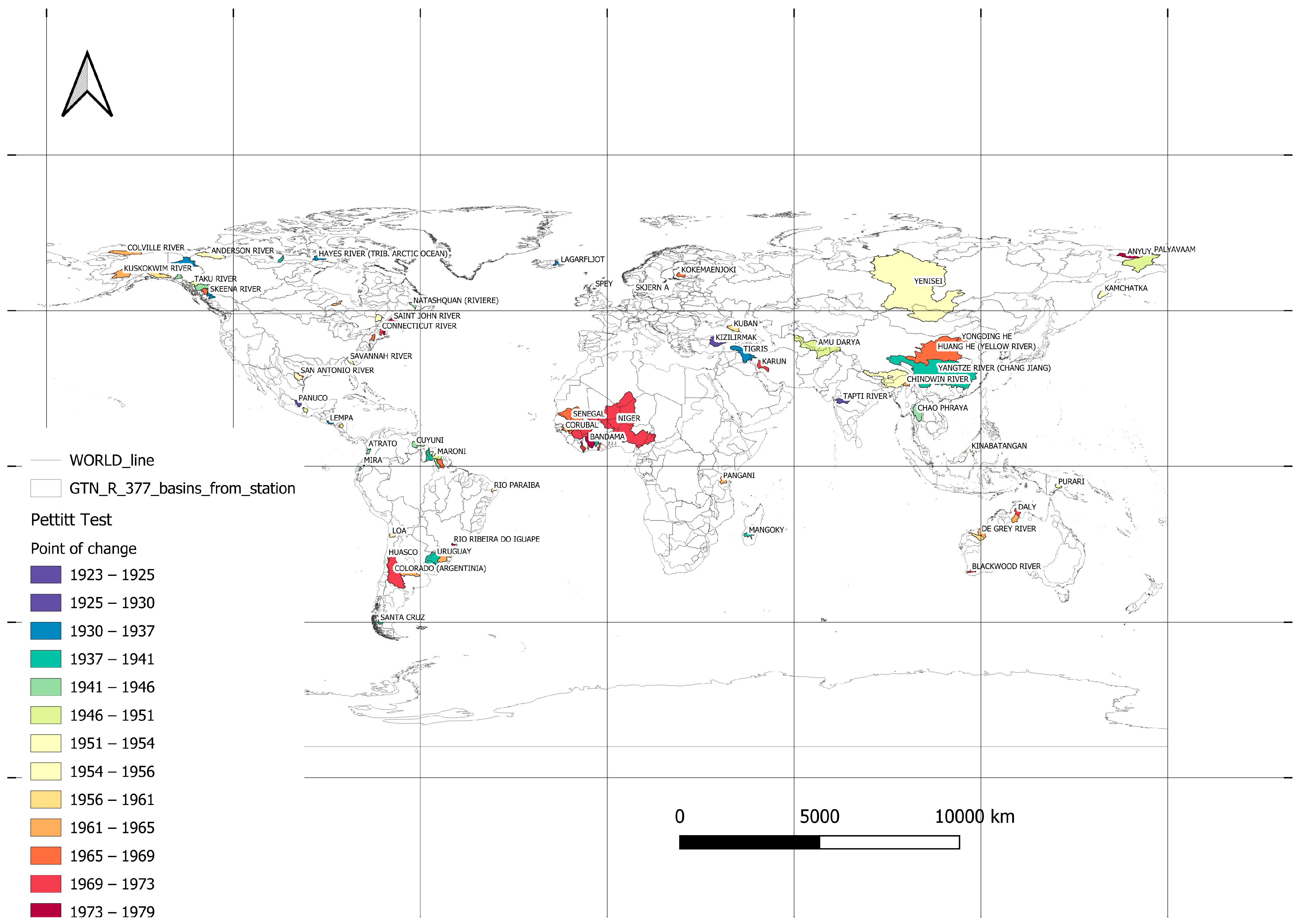
6. Detecting a Change Point in the Trend
7. Trend Test
8. Results and Discussion
- Determining the values of long-term monthly series over a 110-year period;
- Calculating statistics related to the average values for each calendar month, including the minimum, maximum, mean, and standard deviation;
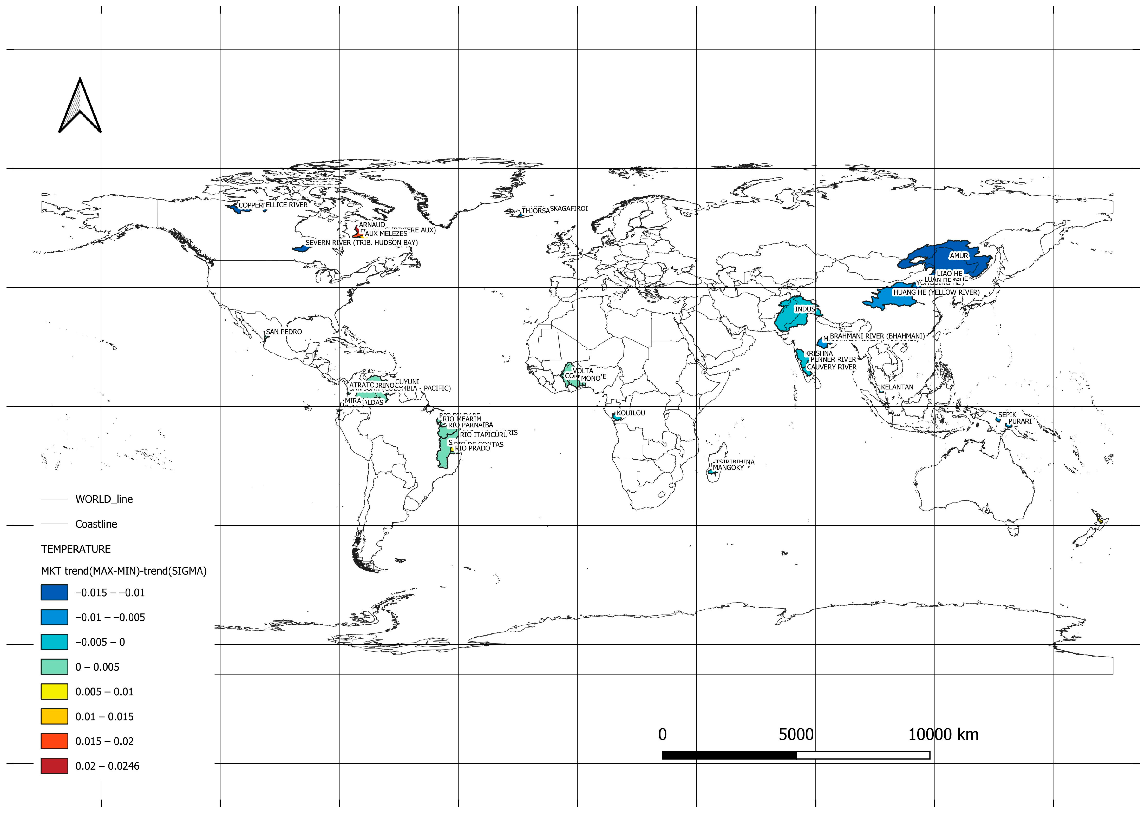
- Determining trend values using the Mann–Kendall test (MKT) to evaluate trends;
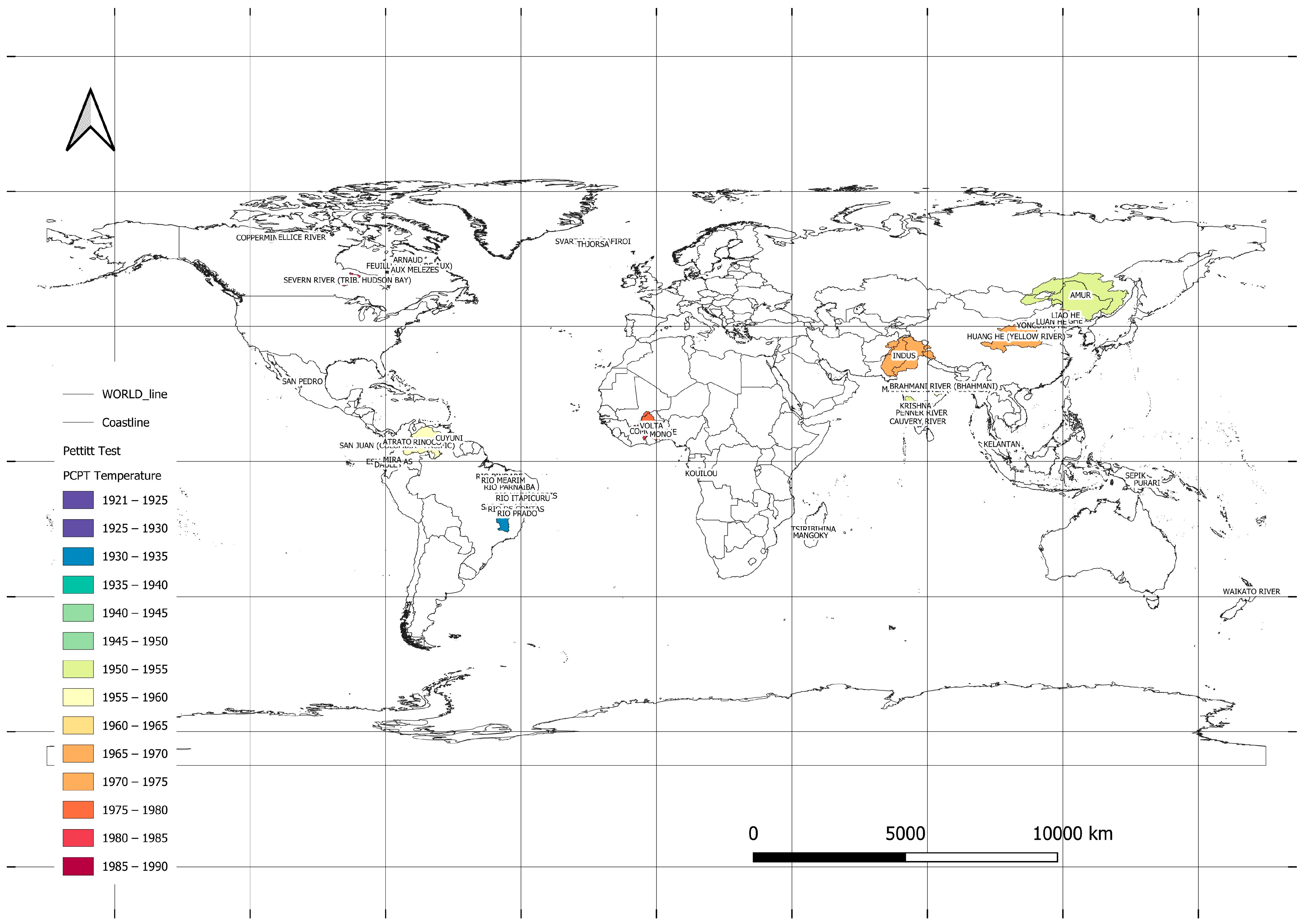
- Examining whether the long-term series exhibited change points using the Pettitt test (PCPT);
- Investigating whether the sub-series (after the identified change point up to 2010) showed a significant trend and how this trend differed from the long-term series in cases where change points were identified.
- Asia: diversity of topography can affect air mass movements and precipitation formation; changes in atmospheric circulation such as monsoons; increasing urbanisation and infrastructure development can create the so-called “heat island effect”, which affects the microclimate; air pollution including particulate matter, which affects condensation and cloud formation [31,128];
- South America: atmospheric circulation fluctuations, including those associated with El Niño and La Niña; topography of the region, including the Andes; deforestation; conversion of land for agriculture and urbanisation [46];
- Australia and Oceania: El Niño–La Niña cycle, changes in ocean circulation, variation in ocean surface temperature and atmospheric pressure between western and eastern areas of the Indian Ocean, deforestation, change in water use and air pollution, intensive agriculture, and overexploitation of water resources [31,46].
9. Conclusions
Funding
Institutional Review Board Statement
Informed Consent Statement
Data Availability Statement
Conflicts of Interest
References
- Romanowicz, R.J.; Bogdanowicz, E.; Debele, S.E.; Doroszkiewicz, J.; Hisdal, H.; Lawrence, D.; Meresa, H.K.; Napiórkowski, J.J.; Osuch, M.; Strupczewski, W.G.; et al. Climate Change Impact on Hydrological Extremes: Preliminary Results from the Polish-Norwegian Project. Acta Geophys. 2016, 64, 477–509. [Google Scholar] [CrossRef]
- Palaniswami, S.; Muthiah, K. Change Point Detection and Trend Analysis of Rainfall and Temperature Series over the Vellar River Basin. Polish J. Environ. Stud. 2018, 27, 1673–1682. [Google Scholar] [CrossRef] [PubMed]
- Groves, D.G.; Yates, D.; Tebaldi, C. Developing and Applying Uncertain Global Climate Change Projections for Regional Water Management Planning. Water Resour. Res. 2008, 44, 1–16. [Google Scholar] [CrossRef]
- Katz, R. Statistics of Extremes in Climatology and Hydrology. Adv. Water Resour. 2002, 25, 1287–1304. [Google Scholar] [CrossRef]
- Herschy, R.W. The World’s Maximum Observed Floods. Flow Meas. Instrum. 2002, 13, 231–235. [Google Scholar] [CrossRef]
- Blöschl, G.; Bierkens, M.F.P.; Chambel, A.; Cudennec, C.; Destouni, G.; Fiori, A.; Kirchner, J.W.; McDonnell, J.J.; Savenije, H.H.G.; Sivapalan, M.; et al. Twenty-Three Unsolved Problems in Hydrology (UPH)—A Community Perspective. Hydrol. Sci. J. 2019, 64, 1141–1158. [Google Scholar] [CrossRef]
- Lewis, S.C.; King, A.D. Evolution of Mean, Variance and Extremes in 21st Century Temperatures. Weather Clim. Extrem. 2017, 15, 1–10. [Google Scholar] [CrossRef]
- Jaiswal, R.K.; Lohani, A.K.; Tiwari, H.L. Statistical Analysis for Change Detection and Trend Assessment in Climatological Parameters. Environ. Process. 2015, 2, 729–749. [Google Scholar] [CrossRef]
- Heim, R.R. An Overview of Weather and Climate Extremes—Products and Trends. Weather Clim. Extrem. 2015, 10, 1–9. [Google Scholar] [CrossRef]
- Sillmann, J.; Thorarinsdottir, T.; Keenlyside, N.; Schaller, N.; Alexander, L.V.; Hegerl, G.; Seneviratne, S.I.; Vautard, R.; Zhang, X.; Zwiers, F.W. Understanding, Modeling and Predicting Weather and Climate Extremes: Challenges and Opportunities. Weather Clim. Extrem. 2017, 18, 65–74. [Google Scholar] [CrossRef]
- Młyński, D.; Cebulska, M.; Wałȩga, A. Trends, Variability, and Seasonality of Maximum Annual Daily Precipitation in the Upper Vistula Basin, Poland. Atmosphere 2018, 9, 313. [Google Scholar] [CrossRef]
- Młyński, D.; Wałȩga, A.; Petroselli, A.; Tauro, F.; Cebulska, M. Estimating Maximum Daily Precipitation in the Upper Vistula Basin, Poland. Atmosphere 2019, 10, 43. [Google Scholar] [CrossRef]
- Twardosz, R.C.M. Temporal Variability of Maximum Monthly Precipitation Totals in the Polish Western Carpathian Mts during the Period 1951–2005. Pr. Geogr. 2012, 128, 123–134. [Google Scholar] [CrossRef]
- Ziernicka-Wojtaszek, A.; Kopcińska, J. Variation in Atmospheric Precipitation in Poland in the Years 2001–2018. Atmosphere 2020, 11, 794. [Google Scholar] [CrossRef]
- Venegas-Cordero, N.; Kundzewicz, Z.W.; Jamro, S.; Piniewski, M. Detection of Trends in Observed River Floods in Poland. J. Hydrol. Reg. Stud. 2022, 41, 101098. [Google Scholar] [CrossRef]
- Kundzewicz, Z.W.; Radziejewski, M. Methodologies for Trend Detection. IAHS-AISH Publ. 2006, 308, 538–549. [Google Scholar]
- Kundzewicz, Z.W.; Robson, A. Detecting Trend and Other Changes in Hydrological Data. World Clim. Program.-Water 2000, 1013, 158. [Google Scholar]
- Berezowski, T.; Szczeniak, M.; Kardel, I.; Michalowski, R.; Okruszko, T.; Mezghani, A.; Piniewski, M. CPLFD-GDPT5: High-Resolution Gridded Daily Precipitation and Temperature Data Set for Two Largest Polish River Basins. Earth Syst. Sci. Data 2016, 8, 127–139. [Google Scholar] [CrossRef]
- Twaróg, B. Characteristics of Multi-Annual Variation of Precipitation in Areas Particularly Exposed to Extreme Phenomena. Part 1. the Upper Vistula River Basin. E3S Web Conf. 2018, 49, 00121. [Google Scholar] [CrossRef]
- Yu, Y.; He, F.; Vavrus, S.J.; Johnson, A.; Wu, H.; Zhang, W.; Yin, Q.; Ge, J.; Deng, C.; Petraglia, M.D.; et al. Climatic Factors and Human Population Changes in Eurasia between the Last Glacial Maximum and the Early Holocene. Glob. Planet. Change 2023, 221, 104054. [Google Scholar] [CrossRef]
- Chen, T.; Zou, L.; Xia, J.; Liu, H.; Wang, F. Decomposing the Impacts of Climate Change and Human Activities on Runoff Changes in the Yangtze River Basin: Insights from Regional Differences and Spatial Correlations of Multiple Factors. J. Hydrol. 2022, 615, 128649. [Google Scholar] [CrossRef]
- Szolgayova, E.; Parajka, J.; Blöschl, G.; Bucher, C. Long Term Variability of the Danube River Flow and Its Relation to Precipitation and Air Temperature. J. Hydrol. 2014, 519, 871–880. [Google Scholar] [CrossRef]
- Pechlivanidis, I.G.; Olsson, J.; Bosshard, T.; Sharma, D.; Sharma, K.C. Multi-Basin Modelling of Future Hydrological Fluxes in the Indian Subcontinent. Water 2016, 8, 177. [Google Scholar] [CrossRef]
- Mudelsee, M.; Börngen, M.; Tetzlaff, G.; Grünewald, U. Extreme Floods in Central Europe over the Past 500 Years: Role of Cyclone Pathway ‘Zugstrasse Vb’. J. Geophys. Res. D Atmos. 2004, 109, D23101. [Google Scholar] [CrossRef]
- Vavrus, S.J.; Notaro, M.; Lorenz, D.J. Interpreting Climate Model Projections of Extreme Weather Events. Weather Clim. Extrem. 2015, 10, 10–28. [Google Scholar] [CrossRef]
- Angélil, O.; Perkins-Kirkpatrick, S.; Alexander, L.V.; Stone, D.; Donat, M.G.; Wehner, M.; Shiogama, H.; Ciavarella, A.; Christidis, N. Comparing Regional Precipitation and Temperature Extremes in Climate Model and Reanalysis Products. Weather Clim. Extrem. 2016, 13, 35–43. [Google Scholar] [CrossRef]
- Michaelides, S.; Levizzani, V.; Anagnostou, E.; Bauer, P.; Kasparis, T.; Lane, J.E. Precipitation: Measurement, Remote Sensing, Climatology and Modeling. Atmos. Res. 2009, 94, 512–533. [Google Scholar] [CrossRef]
- Das, N.; Bhattacharjee, R.; Choubey, A.; Ohri, A.; Dwivedi, S.B.; Gaur, S. Time Series Analysis of Automated Surface Water Extraction and Thermal Pattern Variation over the Betwa River, India. Adv. Sp. Res. 2021, 68, 1761–1788. [Google Scholar] [CrossRef]
- Reinking, R.F. An Approach to Remote Sensing and Numerical Modeling of Orographic Clouds and Precipitation for Climatic Water Resources Assessment. Atmos. Res. 1995, 35, 349–367. [Google Scholar] [CrossRef]
- López-Bermeo, C.; Montoya, R.D.; Caro-Lopera, F.J.; Díaz-García, J.A. Validation of the Accuracy of the CHIRPS Precipitation Dataset at Representing Climate Variability in a Tropical Mountainous Region of South America. Phys. Chem. Earth Parts A/B/C 2022, 127, 103184. [Google Scholar] [CrossRef]
- Becker, A.; Finger, P.; Meyer-Christoffer, A.; Rudolf, B.; Schamm, K.; Schneider, U.; Ziese, M. A Description of the Global Land-Surface Precipitation Data Products of the Global Precipitation Climatology Centre with Sample Applications Including Centennial (Trend) Analysis from 1901-Present. Earth Syst. Sci. Data 2013, 5, 71–99. [Google Scholar] [CrossRef]
- Gómez, J.D.; Etchevers, J.D.; Monterroso, A.I.; Gay, C.; Campo, J.; Martínez, M. Spatial Estimation of Mean Temperature and Precipitation in Areas of Scarce Meteorological Information. Atmosfera 2008, 21, 35–56. [Google Scholar]
- Easterling, D.R.; Kunkel, K.E.; Wehner, M.F.; Sun, L. Detection and Attribution of Climate Extremes in the Observed Record. Weather Clim. Extrem. 2016, 11, 17–27. [Google Scholar] [CrossRef]
- Guimares Nobre, G.; Jongman, B.; Aerts, J.; Ward, P.J. The Role of Climate Variability in Extreme Floods in Europe. Environ. Res. Lett. 2017, 12, 084012. [Google Scholar] [CrossRef]
- Petrow, T.; Merz, B. Trends in Flood Magnitude, Frequency and Seasonality in Germany in the Period 1951–2002. J. Hydrol. 2009, 371, 129–141. [Google Scholar] [CrossRef]
- Singh, P.; Gupta, A.; Singh, M. Hydrological Inferences from Watershed Analysis for Water Resource Management Using Remote Sensing and GIS Techniques. Egypt. J. Remote Sens. Sp. Sci. 2014, 17, 111–121. [Google Scholar] [CrossRef]
- Zhang, X.; Vincent, L.A.; Hogg, W.D.; Niitsoo, A. Temperature and Precipitation Trends in Canada during the 20th Century. Atmos.-Ocean 2000, 38, 395–429. [Google Scholar] [CrossRef]
- Karmeshu, N. Trend Detection in Annual Temperature & Precipitation Using the Mann Kendall Test—A Case Study to Assess Climate Change on Select States in the Northeastern United States. Mausam 2015, 66, 1–6. [Google Scholar]
- Dankers, R.; Hiederer, R. Extreme Temperatures and Precipitation in Europe: Analysis of a High-Resolution Climate Change Scenario. JRC Sci. Tech. Rep. 2008, EUR 23291, 82. Available online: https://www.semanticscholar.org/paper/Extreme-Temperatures-and-Precipitation-in-Europe%3A-a-Rutger-Roland/05a831272412d5e53311e230bf171ff5f63f1751 (accessed on 14 April 2023).
- Katz, R.W.; Parlange, M.B. Overdispersion Phenomenon in Stochastic Modeling of Precipitation. J. Clim. 1998, 11, 591–601. [Google Scholar] [CrossRef]
- Roy, S.S.; Balling, R.C. Trends in Extreme Daily Precipitation Indices in India. Int. J. Climatol. 2004, 24, 457–466. [Google Scholar] [CrossRef]
- Colmet-Daage, A.; Sanchez-Gomez, E.; Ricci, S.; Llovel, C.; Estupina, V.B.; Quintana-Seguí, P.; Carmen Llasat, M.; Servat, E. Evaluation of Uncertainties in Mean and Extreme Precipitation under Climate Change for Northwestern Mediterranean Watersheds from High-Resolution Med and Euro-CORDEX Ensembles. Hydrol. Earth Syst. Sci. 2018, 22, 673–687. [Google Scholar] [CrossRef]
- Bernstein, L.; Bosch, P.; Canziani, O.; Chen, Z.; Christ, R.; Davidson, O.; Hare, W.; Huq, S.; Karoly, D.; Kattsov, V.; et al. Climate Change 2007: An Assessment of the Intergovernmental Panel on Climate Change. Change 2007, 446, 12–17. [Google Scholar]
- Pitt, M.A. Increased Temperature and Entropy Production in the Earth’s Atmosphere: Effect on Wind, Precipitation, Chemical Reactions, Freezing and Melting of Ice and Electrical Activity. J. Mod. Phys. 2019, 10, 966–973. [Google Scholar] [CrossRef]
- Knoben, W.J.M.; Woods, R.A.; Freer, J.E. Global Bimodal Precipitation Seasonality: A Systematic Overview. Int. J. Climatol. 2019, 39, 558–567. [Google Scholar] [CrossRef]
- WMO Guide to Climatological Practices 2018 Edition; WMO: Geneva, Switzerland, 2018; ISBN 9789263101006.
- Ross, S.M. Introduction to Probability and Statistics; Elsevier: Amsterdam, The Netherlands, 2014; ISBN 978-0-12-394811-3. [Google Scholar]
- Hao, Z. Application of Entropy Theory in Hydrologic Analysis and Simulation. Ph.D. Thesis, Texas A&M University, College Station, TX, USA, May 2016. [Google Scholar]
- Rica, C. Tropical Meteorology Research Programme (Tmrp) Commission for Atmospheric Sciences (CAS). Int. Organ. 2006, 16, 241–243. [Google Scholar] [CrossRef]
- Kuhlman, T.; Farrington, J. What Is Sustainability? Sustainability 2010, 2, 3436–3448. [Google Scholar] [CrossRef]
- Eizenberg, E.; Jabareen, Y. Social Sustainability: A New Conceptual Framework. Sustainability 2017, 9, 68. [Google Scholar] [CrossRef]
- McCormick, K.; Kautto, N. The Bioeconomy in Europe: An Overview. Sustainability 2013, 5, 2589–2608. [Google Scholar] [CrossRef]
- Velten, S.; Leventon, J.; Jager, N.; Newig, J. What Is Sustainable Agriculture? A Systematic Review. Sustainability 2015, 7, 7833–7865. [Google Scholar] [CrossRef]
- Lewandowski, M. Designing the Business Models for Circular Economy-towards the Conceptual Framework. Sustainability 2016, 8, 43. [Google Scholar] [CrossRef]
- Staffas, L.; Gustavsson, M.; McCormick, K. Strategies and Policies for the Bioeconomy and Bio-Based Economy: An Analysis of Official National Approaches. Sustainability 2013, 5, 2751–2769. [Google Scholar] [CrossRef]
- Müller, J.M.; Kiel, D.; Voigt, K.I. What Drives the Implementation of Industry 4.0? The Role of Opportunities and Challenges in the Context of Sustainability. Sustainability 2018, 10, 247. [Google Scholar] [CrossRef]
- Lahti, T.; Wincent, J.; Parida, V. A Definition and Theoretical Review of the Circular Economy, Value Creation, and Sustainable Business Models: Where Are We Now and Where Should Research Move in the Future? Sustainability 2018, 10, 2799. [Google Scholar] [CrossRef]
- Schaubroeck, T.; Schaubroeck, S.; Heijungs, R.; Zamagni, A.; Brandão, M.; Benetto, E. Attributional & Consequential Life Cycle Assessment: Definitions, Conceptual Characteristics and Modelling Restrictions. Sustainability 2021, 13, 7386. [Google Scholar] [CrossRef]
- Chapman, J. A Nonparametric Approach to Detecting Changes in Variance in Locally Stationary Time Series. Environmetrics 2020, 31, e2576. [Google Scholar] [CrossRef]
- Thornton, P.K.; Ericksen, P.J.; Herrero, M.; Challinor, A.J. Climate Variability and Vulnerability to Climate Change: A Review. Glob. Change Biol. 2014, 20, 3313–3328. [Google Scholar] [CrossRef]
- Swanson, K.L.; Tsonis, A.A. Has the Climate Recently Shifted? Geophys. Res. Lett. 2009, 36, L06711. [Google Scholar] [CrossRef]
- Balhane, S.; Driouech, F.; Chafki, O.; Manzanas, R.; Chehbouni, A.; Moufouma-Okia, W. Changes in Mean and Extreme Temperature and Precipitation Events from Different Weighted Multi-Model Ensembles over the Northern Half of Morocco. Clim. Dyn. 2022, 58, 389–404. [Google Scholar] [CrossRef]
- Mesbahzadeh, T.; Miglietta, M.M.; Mirakbari, M.; Soleimani Sardoo, F.; Abdolhoseini, M. Joint Modeling of Precipitation and Temperature Using Copula Theory for Current and Future Prediction under Climate Change Scenarios in Arid Lands (Case Study, Kerman Province, Iran). Adv. Meteorol. 2019, 2019, 6848049. [Google Scholar] [CrossRef]
- Gerten, D.; Rost, S.; von Bloh, W.; Lucht, W. Causes of Change in 20th Century Global River Discharge. Geophys. Res. Lett. 2008, 35, 1–5. [Google Scholar] [CrossRef]
- Walling, D.E. Human Impact on Land–Ocean Sediment Transfer by the World’s Rivers. Geomorphology 2006, 79, 192–216. [Google Scholar] [CrossRef]
- Hunter, T.S.; Clites, A.H.; Campbell, K.B.; Gronewold, A.D. Development and Application of a North American Great Lakes Hydrometeorological Database—Part I: Precipitation, Evaporation, Runoff, and Air Temperature. J. Great Lakes Res. 2015, 41, 65–77. [Google Scholar] [CrossRef]
- Chai, Y.; Yue, Y.; Zhang, L.; Miao, C.; Borthwick, A.G.L.; Zhu, B.; Li, Y.; Dolman, A.J. Homogenization and Polarization of the Seasonal Water Discharge of Global Rivers in Response to Climatic and Anthropogenic Effects. Sci. Total Environ. 2020, 709, 136062. [Google Scholar] [CrossRef] [PubMed]
- Li, Z.; Shi, Y.; Argiriou, A.A.; Ioannidis, P.; Mamara, A.; Yan, Z. A Comparative Analysis of Changes in Temperature and Precipitation Extremes since 1960 between China and Greece. Atmosphere 2022, 13, 1824. [Google Scholar] [CrossRef]
- Jahn, M. Economics of Extreme Weather Events: Terminology and Regional Impact Models. Weather Clim. Extrem. 2015, 10, 29–39. [Google Scholar] [CrossRef]
- Zhang, X.; Alexander, L.; Hegerl, G.C.; Jones, P.; Tank, A.K.; Peterson, T.C.; Trewin, B.; Zwiers, F.W. Indices for Monitoring Changes in Extremes Based on Daily Temperature and Precipitation Data. Wiley Interdiscip. Rev. Clim. Change 2011, 2, 851–870. [Google Scholar] [CrossRef]
- Allan, R.P.; Soden, B.J. Atmospheric Warming and the Amplification of Precipitation Extremes. Science 2008, 321, 1481–1484. [Google Scholar] [CrossRef]
- Christensen, J.H.; Kanikicharla, K.K.; Aldrian, E.; An, S.I.; Albuquerque Cavalcanti, I.F.; de Castro, M.; Dong, W.; Goswami, P.; Hall, A.; Kanyanga, J.K.; et al. Climate Phenomena and Their Relevance for Future Regional Climate Change. In Climate Change 2013—The Physical Science Basis; Working Group I Contribution to the Fifth Assessment Report of the Intergovernmental Panel on Climate Change; Cambridge University Press: Cambridge, UK, 2013; Volume 9781107057, pp. 1217–1308. [Google Scholar] [CrossRef]
- Cardona, O.D.; Van Aalst, M.K.; Birkmann, J.; Fordham, M.; Mc Gregor, G.; Rosa, P.; Pulwarty, R.S.; Schipper, E.L.F.; Sinh, B.T.; Décamps, H.; et al. Determinants of Risk: Exposure and Vulnerability. In Managing the Risks of Extreme Events and Disasters to Advance Climate Change Adaptation; Special Report of the Intergovernmental Panel on Climate Change; Cambridge University Press: Cambridge, UK, 2012; Volume 9781107025, pp. 65–108. [Google Scholar] [CrossRef]
- Kolokytha, E.; Oishi, S.; Teegavarapu, R.S.V. Sustainable Water Resources Planning and Management under Climate Change; Kolokytha, E., Ed.; Springer Science+Business Media: Singapore, 2016; ISBN 9789811020513. [Google Scholar]
- Powell, J.P.; Reinhard, S. Measuring the Effects of Extreme Weather Events on Yields. Weather Clim. Extrem. 2015, 12, 69–79. [Google Scholar] [CrossRef]
- Lal, P.N.; Mitchell, T.; Aldunce, P.; Auld, H.; Mechler, R.; Miyan, A.; Romano, L.E.; Zakaria, S.; Dlugolecki, A.; Masumoto, T.; et al. National Systems for Managing the Risks from Climate Extremes and Disasters; Cambridge University Press: Cambridge, UK, 2012; Volume 9781107025, ISBN 9781139177245. [Google Scholar]
- Knapp, A.K.; Beier, C.; Briske, D.D.; Classen, A.T.; Yiqi, L.; Reichstein, M.; Smith, M.D.; Smith, S.D.; Bell, J.E.; Fay, P.A.; et al. Consequences of More Extreme Precipitation Regimes for Terrestrial Ecosystems. Bioscience 2008, 58, 811–821. [Google Scholar] [CrossRef]
- Sitthiyot, T.; Holasut, K. A Simple Method for Measuring Inequality. Palgrave Commun. 2020, 6, 112. [Google Scholar] [CrossRef]
- Vermeulen, S.J.; Challinor, A.J.; Thornton, P.K.; Campbell, B.M.; Eriyagama, N.; Vervoort, J.M.; Kinyangi, J.; Jarvis, A.; Läderach, P.; Ramirez-Villegas, J.; et al. Addressing Uncertainty in Adaptation Planning for Agriculture. Proc. Natl. Acad. Sci. USA 2013, 110, 8357–8362. [Google Scholar] [CrossRef] [PubMed]
- Ramirez-Villegas, J.; Lau, C.; Köhler, A.K.; Signer, J.; Jarvis, A.; Arnell, N.W.; Osborne, T.M.; Hooker, J. Climate Analogues: Finding Tomorrow’s Agriculture Today. Work. Pap. No. 12 2011, 12, 40. [Google Scholar]
- Matos, S.; Viardot, E.; Sovacool, B.K.; Geels, F.W.; Xiong, Y. Innovation and Climate Change: A Review and Introduction to the Special Issue. Technovation 2022, 117, 102612. [Google Scholar] [CrossRef]
- Pfleiderer, P.; Schleussner, C.F.; Mengel, M.; Rogelj, J. Global Mean Temperature Indicators Linked to Warming Levels Avoiding Climate Risks. Environ. Res. Lett. 2018, 13, 059501. [Google Scholar] [CrossRef]
- Stephan, G. Intergenerational Fairness and Climate Change Adaptation Policy: An Economic Analysis. Green Low-Carbon Econ. 2023, 1, 105–109. [Google Scholar] [CrossRef]
- Langdon, J.G.R.; Lawler, J.J. Assessing the Impacts of Projected Climate Change on Biodiversity in the Protected Areas of Western North America. Ecosphere 2015, 6, 1–14. [Google Scholar] [CrossRef]
- Nicolli, F.; Gilli, M.; Vona, F. Inequality and Climate Change: Two Problems, One Solution. Fond. Eni Enrico Mattei Inequal. 2023. [Google Scholar] [CrossRef]
- Twaróg, B. Application of Shannon Entropy in Precipitation Conditions and Application of Shannon Entropy in Assessing Changes in Precipitation Conditions and Temperature Based on Long-Term Sequences Using the Bootstrap Method. Atmosphere 2024, 15, 898. [Google Scholar] [CrossRef]
- Hosseinzadehtalaei, P.; Tabari, H.; Willems, P. Climate Change Impact on Short-Duration Extreme Precipitation and Intensity–Duration–Frequency Curves over Europe. J. Hydrol. 2020, 590, 125249. [Google Scholar] [CrossRef]
- Persson, J.; Blennow, K.; Gonçalves, L.; Borys, A.; Dutca, I.; Hynynen, J.; Janeczko, E.; Lyubenova, M.; Martel, S.; Merganic, J.; et al. No Polarization-Expected Values of Climate Change Impacts among European Forest Professionals and Scientists. Sustainability 2020, 12, 2659. [Google Scholar] [CrossRef]
- Rudolf, B.; Beck, C.; Grieser, J.; Schneider, U. Global Precipitation Analysis Products of the GPCC. Internet Publ. 2005, 112, 3819–3837. [Google Scholar]
- Arheimer, B.; Pimentel, R.; Isberg, K.; Crochemore, L.; Andersson, J.C.M.; Hasan, A.; Pineda, L. Global Catchment Modelling Using World-Wide HYPE (WWH), Open Data, and Stepwise Parameter Estimation. Hydrol. Earth Syst. Sci. 2020, 24, 535–559. [Google Scholar] [CrossRef]
- Iverson, L.R.; McKenzie, D. Tree-Species Range Shifts in a Changing Climate: Detecting, Modeling, Assisting. Landsc. Ecol. 2013, 28, 879–889. [Google Scholar] [CrossRef]
- Franklin, J. Mapping Species Distributions: Spatial Inference and Prediction. Oryx 2010, 44, 615. [Google Scholar] [CrossRef]
- Viner, D.; Ekstrom, M.; Hulbert, M.; Warner, N.K.; Wreford, A.; Zommers, Z. Understanding the Dynamic Nature of Risk in Climate Change Assessments—A New Starting Point for Discussion. Atmos. Sci. Lett. 2020, 21, e958. [Google Scholar] [CrossRef]
- Rosenzweig, C.; Parry, M. Potential Impact of Climate Change on World Food Supply. Nature 1992, 367, 133–138. [Google Scholar] [CrossRef]
- Tabari, H.; Willems, P. Lagged Influence of Atlantic and Pacific Climate Patterns on European Extreme Precipitation. Sci. Rep. 2018, 8, 5748. [Google Scholar] [CrossRef]
- Gibbins, G.; Haigh, J.D. Entropy Production Rates of the Climate. J. Atmos. Sci. 2020, 77, 3551–3566. [Google Scholar] [CrossRef]
- Kharin, V.V.; Zwiers, F.W.; Zhang, X.; Wehner, M. Changes in Temperature and Precipitation Extremes in the CMIP5 Ensemble. Clim. Change 2013, 119, 345–357. [Google Scholar] [CrossRef]
- Verstraeten, G.; Poesen, J.; Demarée, G.; Salles, C. Long-Term (105 Years) Variability in Rain Erosivity as Derived from 10-Min Rainfall Depth Data for Ukkel (Brussels, Belgium): Implications for Assessing Soil Erosion Rates. J. Geophys. Res. Atmos. 2006, 111, 1–11. [Google Scholar] [CrossRef]
- Lovell, R.S.L.; Blackburn, T.M.; Dyer, E.E.; Pigot, A.L. Environmental Resistance Predicts the Spread of Alien Species. Nat. Ecol. Evol. 2021, 5, 322–329. [Google Scholar] [CrossRef] [PubMed]
- Stocker, T.F.; Clarke, G.K.C.; Le Treut, H.; Lindzen, R.S.; Meleshko, V.P.; Mugara, R.K.; Palmer, T.N.; Pierrehumbert, R.T.; Sellers, P.J.; Trenberth, K.E.; et al. Physical Climate Processes and Feedbacks. In Climate Change 2001: The Scientific Basis; Contribution of Working Group I to the Third Assessment Report of the Intergovernmental Panel on Climate Change; Cambridge University Press: Cambridge, UK, 2001; Volume 881, pp. 419–457. [Google Scholar]
- Chen, L.; Guo, S. Copulas and Its Application in Hydrology and Water Resources; Springer: Singapore, 2019; ISBN 978-981-13-0573-3. [Google Scholar]
- Hou, W.; Yan, P.; Feng, G.; Zuo, D. A 3D Copula Method for the Impact and Risk Assessment of Drought Disaster and an Example Application. Front. Phys. 2021, 9, 656253. [Google Scholar] [CrossRef]
- Santos-Gómez, J.D.; Fontalvo-García, J.S.; Giraldo Osorio, J.D. Validating the University of Delaware’s Precipitation and Temperature Database for Northern South America. Dyna 2015, 82, 86–95. [Google Scholar] [CrossRef]
- Amiel, Y.; Cowell, F. Thinking about Inequality; Cambridge University Press: Cambridge, UK; New York, NY, USA, 1999; ISBN 9780511492266. [Google Scholar]
- Lorenz, M.O. Methods of Measuring the Concentration of Wealth. Publ. Am. Stat. Assoc. 1905, 9, 209–219. [Google Scholar] [CrossRef]
- Mccright, A.M.; Dunlap, R.E. The Politicization of Climate Change and Polarization in the American Public’s Views of Global Warming, 2001–2010. Sociol. Q. 2011, 52, 155–194. [Google Scholar] [CrossRef]
- Ogwang, T. Calculating a Standard Error for the Gini Coefficient: Some Further Results: Reply. Oxf. Bull. Econ. Stat. 2004, 66, 435–437. [Google Scholar] [CrossRef]
- Damgaard, C.; Weiner, J. Describing Inequality in Plant Size or Fecundity. Ecology 2000, 81, 1139. [Google Scholar] [CrossRef]
- Panek, T. Polaryzacja Ekonomiczna w Polsce. Wiadomości. Stat. 2017, 1, 41–62. [Google Scholar]
- Samson, P.-M. Concentration of Measure Principle and Entropy-Inequalities; Springer: New York, NY, USA, 2017; ISBN 9781493970049. [Google Scholar]
- Yitzhaki, S. Gini’s Mean Difference: A Superior Measure of Variability for Non-Normal Gini’s Mean Difference: A Superior Measure of Variability for Non-Normal Distributions. Metron. Lxi 2016, 2, 285–316. [Google Scholar]
- Conceição, P.; Ferreira, P. Young Person’s Guide to the Theil Index: Suggesting Intuitive Interpretations and Exploring Analytical Applications. World 2000, 1–54. [Google Scholar] [CrossRef]
- Buishand, T.A. Some Methods for Testing the Homogeneity of Rainfall Records. J. Hydrol. 1982, 58, 11–27. [Google Scholar] [CrossRef]
- Chen, J.; Gupta, A.K. Parametric Statistical Change Point Analysis. 2013–2015. Angew. Chemie Int. Ed. 2021, 6, 951–952. [Google Scholar] [CrossRef]
- Radziejewski, M.; Bardossy, A.; Kundzewicz, Z.W. Detection of Change in River Flow Using Phase Randomization. Hydrol. Sci. J. 2000, 45, 547–558. [Google Scholar] [CrossRef]
- Salarijazi, M. Trend and Change-Point Detection for the Annual Stream-Flow Series of the Karun River at the Ahvaz Hydrometric Station. African J. Agric. Res. 2012, 7, 4540–4552. [Google Scholar] [CrossRef]
- Pettitt, A.N. A Non-Parametric Approach to the Change-Point Problem. J. R. Stat. Soc. Ser. C Appl. Stat. 1979, 28, 126–135. [Google Scholar] [CrossRef]
- Conte, L.C.; Bayer, D.M.; Bayer, F.M. Bootstrap Pettitt Test for Detecting Change Points in Hydroclimatological Data: Case Study of Itaipu Hydroelectric Plant, Brazil. Hydrol. Sci. J. 2019, 64, 1312–1326. [Google Scholar] [CrossRef]
- Mann, H.B. Nonparametric Tests Against Trend. Econometrica 1945, 13, 245–259. [Google Scholar] [CrossRef]
- Yue, S.; Pilon, P.; Phinney, B.; Cavadias, G. The Influence of Autocorrelation on the Ability to Detect Trend in Hydrological Series. Hydrol. Process. 2002, 16, 1807–1829. [Google Scholar] [CrossRef]
- Sen, P.K. Estimates of the Regression Coefficient Based on Kendall’s Tau. J. Am. Stat. Assoc. 1968, 63, 1379–1389. [Google Scholar] [CrossRef]
- Hirsch, R.M.; Slack, J.R.; Smith, R.A. Techniques of Trend Analysis for Monthly Water Quality Data. Water Resour. Res. 1982, 18, 107–121. [Google Scholar] [CrossRef]
- Production and Consumption Gross Energy Consumption by Source. Available online: https://statice.is/statistics/environment/energy/production-and-consumption/ (accessed on 14 April 2023).
- Everett, K.; Hardick, E.; Johnson, D. The Year of Africa; The African Presence; The Ohio State University: Columbus, OH, USA, 2018; pp. 1–24. [Google Scholar] [CrossRef]
- Khanin, G.I. The 1950s: The Triumph of the Soviet Economy. Eur. Asia. Stud. 2003, 55, 1187–1211. [Google Scholar] [CrossRef]
- Levy, M.; Stewart, D.E.; Kent, C.H.W. Encyclopedia Britannica. 2023, pp. 1–15. Available online: https://www.britannica.com/topic/Encyclopaedia-Britannica-English-language-reference-work (accessed on 14 April 2024).
- Love, J.L. The Rise and Decline of Economic Structuralism in Latin America: New Dimensions. Lat. Am. Res. Rev. 2023, 40, 100–125. [Google Scholar] [CrossRef]
- van Eck, C.W.; Mulder, B.C.; Dewulf, A. Online Climate Change Polarization: Interactional Framing Analysis of Climate Change Blog Comments. Sci. Commun. 2020, 42, 454–480. [Google Scholar] [CrossRef]
- Beck, H.E.; Zimmermann, N.E.; McVicar, T.R.; Vergopolan, N.; Berg, A.; Wood, E.F. Present and Future Köppen-Geiger Climate Classification Maps at 1-Km Resolution. Sci. Data 2018, 5, 180214. [Google Scholar] [CrossRef]
- Kottek, M.; Grieser, J.; Beck, C.; Rudolf, B.; Rubel, F. World Map of the Köppen-Geiger Climate Classification Updated. Meteorol. Z. 2006, 15, 259–263. [Google Scholar] [CrossRef] [PubMed]

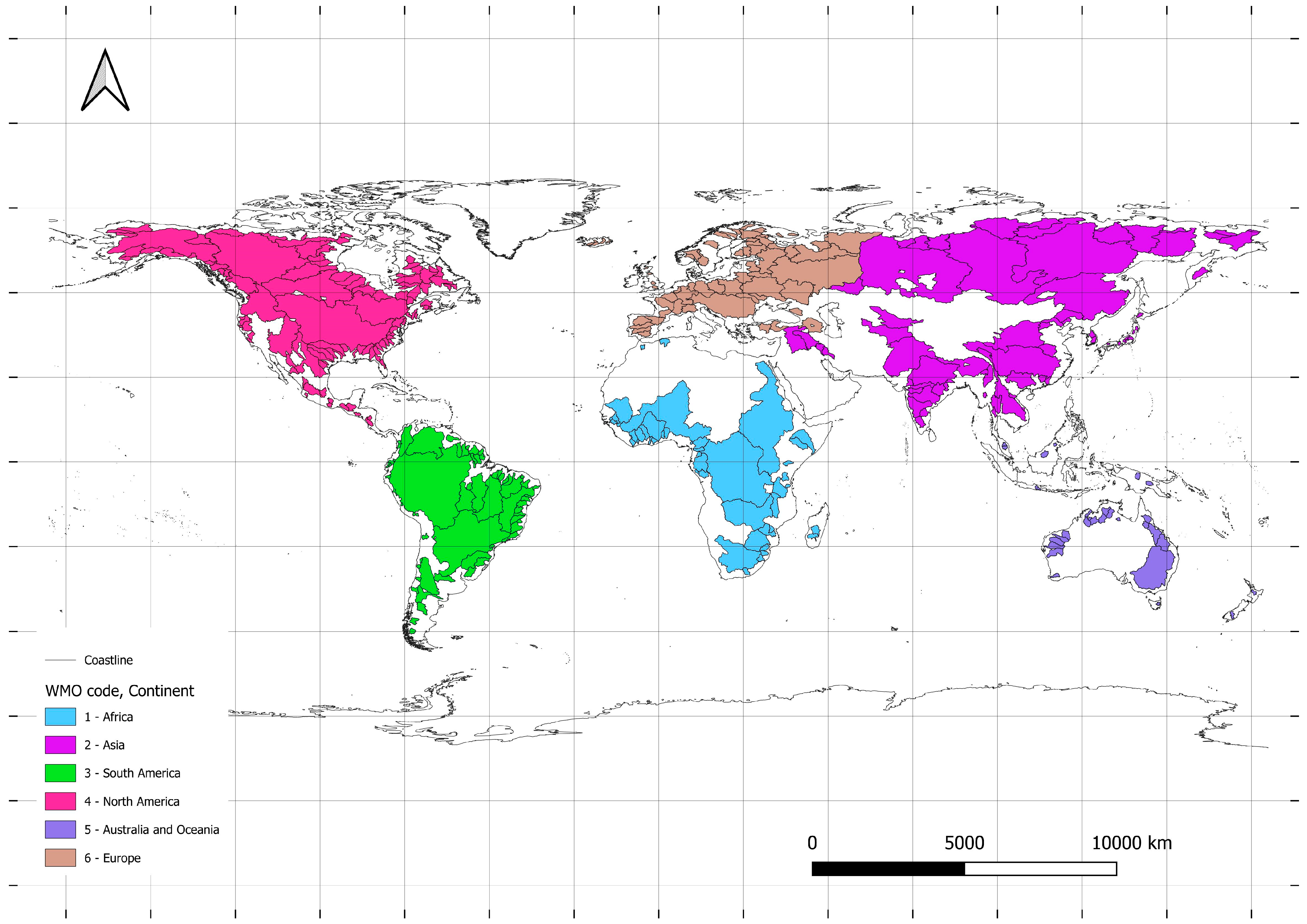
| Region WMO | Continent | Land Area | Area Catchment | Coverage of the Continents |
|---|---|---|---|---|
| WMO_REG | 106 km2 | 106 km2 | % | |
| 1 | Africa | 30.3 | 8.43 | 27.83% |
| 2 | Asia | 44.3 | 20.3 | 45.86% |
| 3 | South America | 17.8 | 12.6 | 70.57% |
| 4 | North America | 24.2 | 13.0 | 53.87% |
| 5 | Australia and Oceania | 8.5 | 1.1 | 13.07% |
| 6 | Europe | 10.5 | 6.7 | 64.10% |
| Antarctica | 13.1 | 0.0 | 0.00% | |
| Total land area | 148.7 | 65.1 | 43.77% | |
| Earth, total | 509.9 | 65.1 | 12.76% |
| Both Values | Impact on Climate Changes |
|---|---|
| Relation: Result: POSITIVE | |
| Increasing range of temperature change: A Trend(Range) value greater than Trend(STD) for temperature suggests that the range of temperature change in an area is increasing over the period under study. This means that the maximum and minimum temperatures in the area vary more than they did previously, which may mean that the temperature varies more over the year or over the years. Increasing range of precipitation changes: Similarly, if the Trend(Range) for precipitation is greater than the Trend(STD) for rainfall, this suggests that the range of precipitation change in the area is also increasing. This may indicate more extreme rainfall conditions or drier periods in the study area. No change in the stability of temperature and precipitation: The Trend(STD) value measures the stability of temperature and precipitation, and the fact that it is positive for both indicators means that variability in these factors in the area is present, but the increase is not as significant as the extent of change. This could mean that there is no clear change in the seasonal or annual patterns of variability in temperature and precipitation, but the extremes are changing. Possible climate change: An increasing range of changes in temperature and precipitation may be a signal of possible climate change in an area. These may be the results of changes in the atmosphere, such as changes in atmospheric circulation or other climatic factors that affect the local climate. | |
| Relation: Result: POSITIVE | |
| Declining range of change in temperature and precipitation: The Trend(Range) value for temperature and Trend(Range) value for precipitation suggest that the range of change in temperature and precipitation in an area is decreasing over the study period. This means that the difference between maximum and minimum temperature and the range of change in precipitation is decreasing. There are no clear trends in the stability of temperature and precipitation: The Trend(STD) value measures the stability of temperature and precipitation, and the fact that it is smaller than the Trend(Range) for these parameters suggests that variability is present but is not as significant as the decreasing range of change. This could mean that the variability in temperature and precipitation in an area remains relatively constant, but the range of variation is decreasing. No clear trend of increasing range: If the Trend(Range) for temperature and Trend(Range) for precipitation are both negative, there are no clear trends to suggest a significant increase in the range of change for these parameters in the area. Potential climate change: A decreasing range of change in temperature and precipitation may be a signal of potential climate change in an area. These may be the results of changes in the atmosphere, such as changes in atmospheric circulation or other climatic factors that affect the local climate. | |
| Relation: Result: NEGATIVE | |
| Stability of the range of change in temperature and precipitation: If the Trend(Range) for temperature and Trend(Range) for precipitation are smaller than the Trend(STD) for these parameters, this suggests that the range of change in temperature and precipitation in the area is more stable or changes less over the time period studied. This means that there is no tendency for the range of temperature and precipitation changes to increase significantly. Stability of temperature and precipitation: The Trend(STD) value measures the stability of temperature and precipitation, and the fact that it is greater than the Trend(Range) for these parameters indicates the presence of variability, but this variability is not as significant as the range of change. This could mean that the variability in temperature and precipitation in the area remains relatively constant. No clear trend of increasing range: If the Trend(Range) for temperature and Trend(Range) for precipitation are less than Trend(STD), there are no clear trends to suggest a significant increase in the range of change of these parameters in the area. Fluctuations around mean values: It is worth noting that although the range of change may be relatively stable, there may still be fluctuations around the mean values of temperature and precipitation in the area. | |
| Relation: Result: NEGATIVE | |
| Declining range of change in temperature and precipitation: The Trend(Range) value for temperature and Trend(Range) value for precipitation suggest that the range of change in temperature and precipitation in an area is decreasing over the study period. This means that the difference between maximum and minimum temperature and the range of change in precipitation is decreasing. Stability of temperature and precipitation: The Trend(STD) value measures the stability of temperature and precipitation, and the fact that it is greater than Trend(Range) for these parameters suggests that variability is present but is not as significant as the decreasing range of change. This could mean that the variability in temperature and precipitation in an area remains relatively constant, but the range of these changes is decreasing. No clear trend of increasing range: If the Trend(Range) for temperature and Trend(Range) for precipitation are both negative, there are no clear trends to suggest a significant increase in the range of change for these parameters in the area. Possible climate change: A decreasing range of change in temperature and precipitation may be a signal of potential climate change in the area. These could be the results of changes in the atmosphere, such as changes in atmospheric circulation or other climatic factors that affect the local climate. | |
| Relation: ZERO | |
| Stability of the range of change in temperature and precipitation: The equality between Trend(Range) and Trend(STD) for temperature and precipitation suggests that the range of changes in temperature and precipitation in an area is relatively stable and does not show a clear tendency to increase or decrease over the study period. Stability of temperature and precipitation: The Trend(STD) value measures the stability of temperature and precipitation, and the fact that it is equal to the Trend(Range) for these parameters indicates the presence of variability, but that this variability is not the dominant trend over the period analysed. This means that the variability in temperature and precipitation in the area remains relatively constant. No clear upward or downward trends: No difference between Trend(Range) and Trend(STD) for temperature and precipitation means that there is no clear trend suggesting a significant increase or decrease in the range of variation in these parameters in the area. Climate stability: Equality between Trend(Range) and Trend(STD) may suggest that the climate in an area is relatively stable over the study period and does not show significant changes in temperature and precipitation. | |
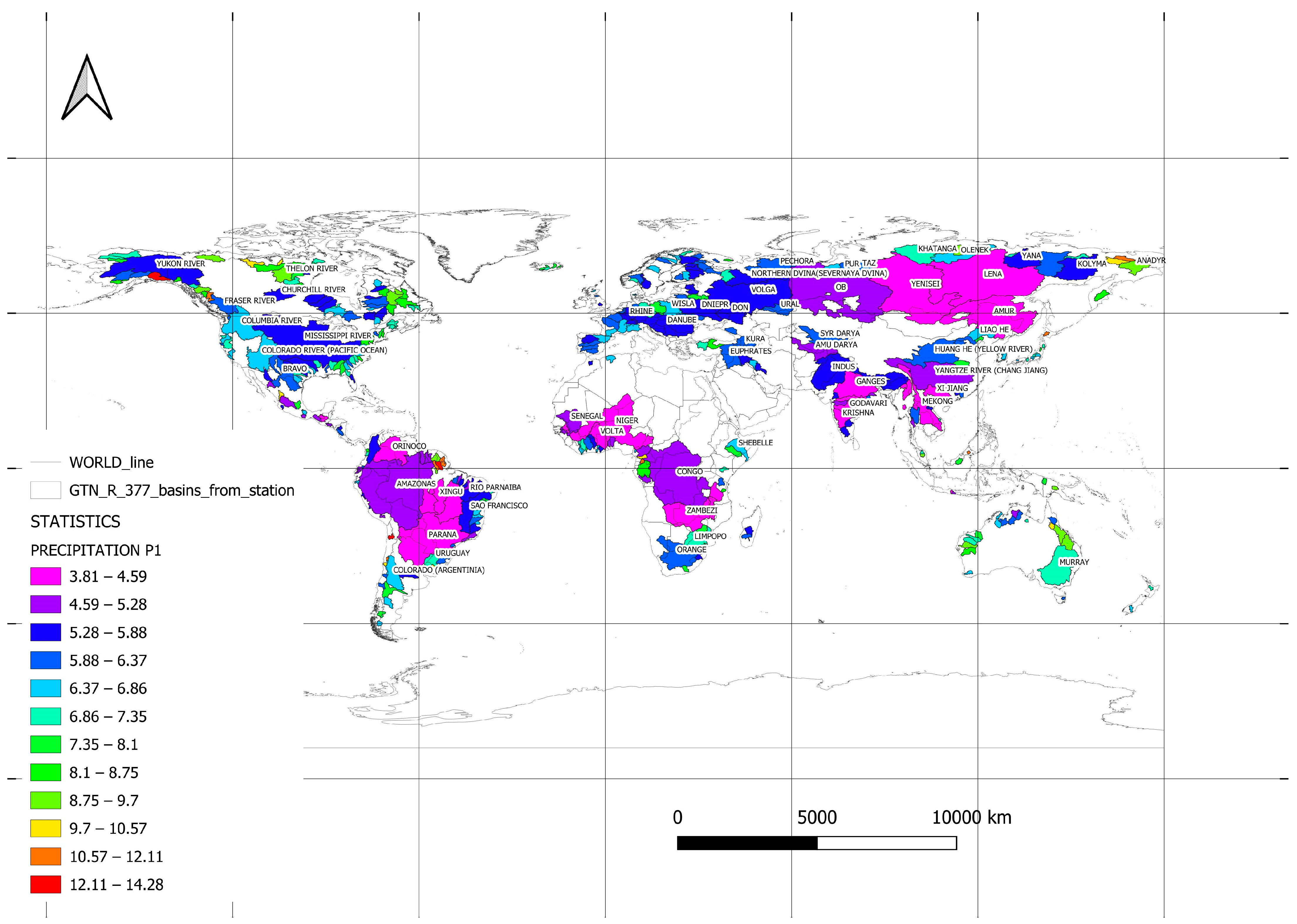
| No | WMO | River | Country | Continent | Area | Cv | P1 |
|---|---|---|---|---|---|---|---|
| [km2] | |||||||
| 138 | 3 | Amazonas | Brazil | South America | 4,640,300 | 0.292 | 4.909 |
| 2 | 1 | Congo | Congo, The De | Africa | 3,475,000 | 0.288 | 5.049 |
| 187 | 4 | Mississippi River | United States | North America | 2,964,255 | 0.412 | 5.536 |
| 94 | 2 | Ob | Russian Fed. | Asia | 2,949,998 | 0.501 | 4.996 |
| 14 | 1 | Nile | Egypt | Africa | 2,900,000 | 0.712 | 4.262 |
| 93 | 2 | Yenisei | Russian Fed. | Asia | 2,440,000 | 0.641 | 4.249 |
| 91 | 2 | Lena | Russian Fed. | Asia | 2,430,000 | 0.731 | 4.570 |
| 125 | 3 | Parana | Argentina | South America | 2,346,000 | 0.582 | 4.529 |
| 92 | 2 | Amur | Russian Fed. | Asia | 1,730,000 | 0.998 | 4.506 |
| 50 | 2 | Yangtze River (Chang Jiang) | China | Asia | 1,705,383 | 0.661 | 5.285 |
| MAX | |||||||
| 180 | 4 | Copper River | United States | North America | 62,678 | 0.710 | 12.781 |
| MIN | |||||||
| 78 | 2 | Ganges | India | Asia | 835,000 | 1.240 | 3.812 |
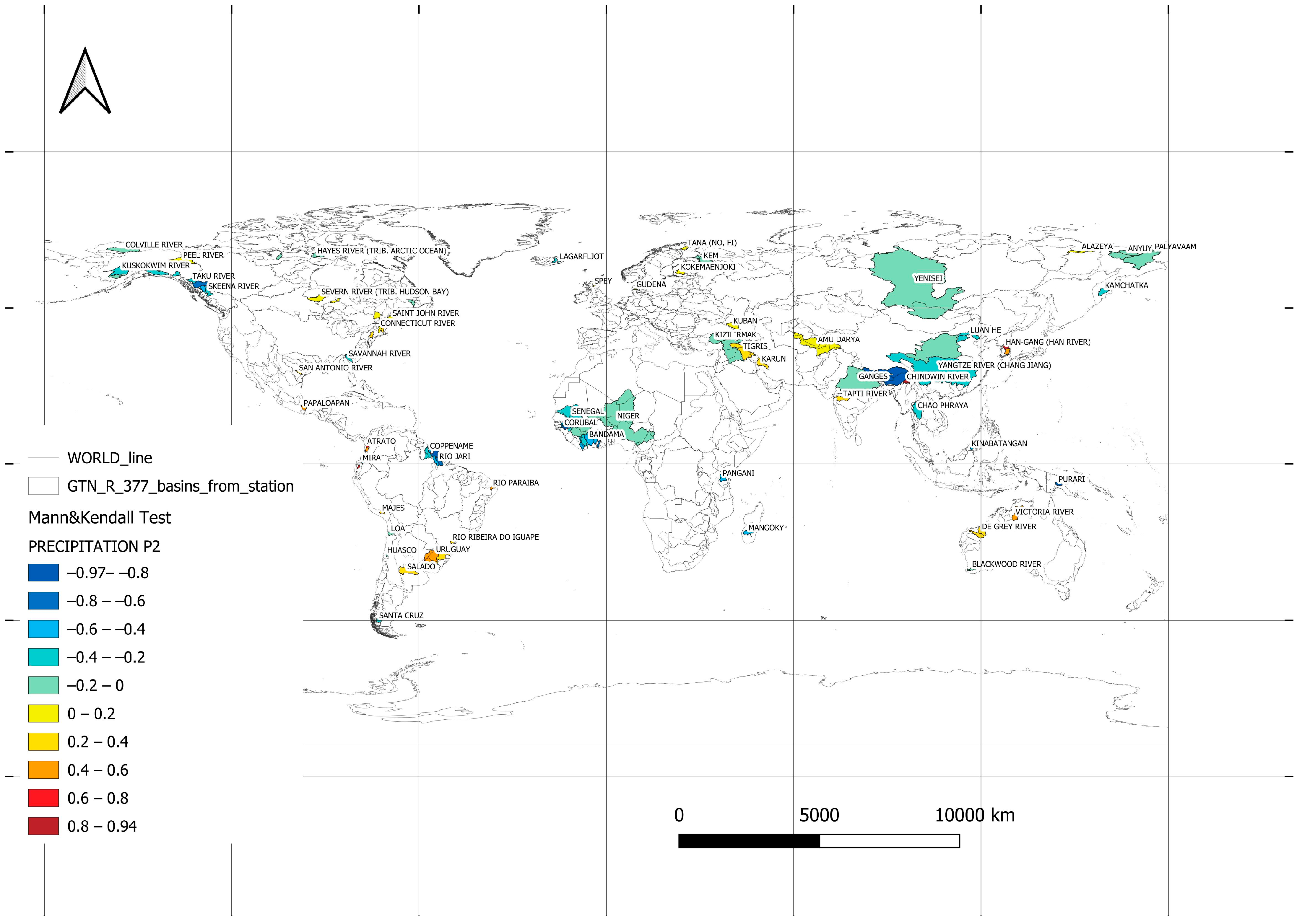
| No | WMO | River | Country | Continent | Area | P2 | Year (STD) | Year (RANGE) |
|---|---|---|---|---|---|---|---|---|
| [km2] | [mm/year] | [year] | [year] | |||||
| 14 | 1 | Nile | Egypt | Africa | 2,900,000 | −0.052 | 1964 | 1967 |
| 93 | 2 | Yenisei | Russian Fed. | Asia | 2,440,000 | −0.053 | 1975 | 1954 |
| 50 | 2 | Yangtze River | China | Asia | 1,705,383 | −0.305 | 1932 | 1939 |
| 78 | 2 | Ganges | India | Asia | 835,000 | −0.170 | ||
| 49 | 2 | Huang He (Yellow River) | China | Asia | 730,036 | −0.151 | ||
| 75 | 2 | Brahmaputra | Bangladesh | Asia | 636,130 | −0.895 | 1955 | 1955 |
| 96 | 2 | Amu Darya | Uzbekistan | Asia | 450,000 | 0.062 | 1947 | 1951 |
| 73 | 2 | Euphrates | Iraq | Asia | 274,100 | −0.103 | ||
| 31 | 1 | Senegal | Senegal | Africa | 268,000 | −0.302 | 1967 | 1967 |
| 135 | 3 | Uruguay | Uruguay | South America | 244,000 | 0.444 | 1945 | 1940 |
| MAX | ||||||||
| 76 | 2 | Han-Gang (Han River) | Korea, Rep. | Asia | 25,046 | 0.945 | 1962 | 1953 |
| MIN | ||||||||
| 295 | 5 | Purari | Papua New Guinea | Australia And Oceania | 11,100 | −0.966 | 1950 | 1950 |
| No | WMO | River | Country | Continent | Area | Cv | P1 |
|---|---|---|---|---|---|---|---|
| [km2] | [] | [] | |||||
| 138 | 3 | Amazonas | Brazil | South America | 4,640,300 | 0.031 | 5.952 |
| 2 | 1 | Congo | The Democratic Republic of Congo | Africa | 3,475,000 | 0.028 | 6.736 |
| 187 | 4 | Mississippi River | United States | North America | 2,964,255 | 1.003 | 3.885 |
| 94 | 2 | Ob | Russian Fed. | Asia | 2,949,998 | −22.694 | 3.820 |
| 14 | 1 | Nile | Egypt | Africa | 2,900,000 | 0.082 | 4.857 |
| 93 | 2 | Yenisei | Russian Fed. | Asia | 2,440,000 | −2.663 | 3.590 |
| 91 | 2 | Lena | Russian Fed. | Asia | 2,430,000 | −1.861 | 3.385 |
| 125 | 3 | Parana | Argentina | South America | 2,346,000 | 0.145 | 4.276 |
| 92 | 2 | Amur | Russian Fed. | Asia | 1,730,000 | −10.070 | 3.420 |
| 50 | 2 | Yangtze River (Chang Jiang) | China | Asia | 1,705,383 | 0.652 | 3.428 |
| MAX | |||||||
| 294 | 5 | Sepik | Papua New Guinea | Australia and Oceania | 40,922 | 0.042 | 10.435 |
| MIN | |||||||
| 102 | 2 | Indigirka | Russian Fed. | Asia | 305,000 | −1.294 | 3.257 |
| No | WMO | River | Country | Continent | Area | P2 | Year (STD) | Year (RANGE) |
|---|---|---|---|---|---|---|---|---|
| [km2] | [°C/year] | [year] | [year] | |||||
| 92 | 2 | Amur | Russian Fed. | Asia | 1,730,000 | −0.018 | 1956 | 1954 |
| 123 | 3 | Orinoco | Venezuela | South America | 836,000 | 0.004 | 1957 | 1957 |
| 58 | 2 | Indus | Pakistan | Asia | 832,418 | −0.006 | 1950 | 1973 |
| 49 | 2 | Huang He (Yellow River) | China | Asia | 730,036 | −0.006 | 1975 | 1971 |
| 156 | 3 | Sao Francisco | Brazil | South America | 622,600 | 0.005 | 1932 | 1932 |
| 25 | 1 | Volta | Ghana | Africa | 394,100 | 0.002 | 1968 | 1978 |
| 152 | 3 | Rio Parnaiba | Brazil | South America | 322,823 | 0.004 | 1958 | 1958 |
| 88 | 2 | Godavari | India | Asia | 299,320 | −0.004 | 1955 | 1955 |
| 87 | 2 | Mahanadi River | India | Asia | 132,090 | −0.009 | 1961 | 1955 |
| 48 | 2 | Liao He | China | Asia | 120,764 | −0.013 | 1957 | 1970 |
| MAX | ||||||||
| 258 | 4 | Arnaud | Canada | North America | 26,900 | 0.022 | 1987 | 1987 |
| MIN | ||||||||
| 92 | 2 | Amur | Russian Fed. | Asia | 1,730,000 | −0.0182 | 1956 | 1954 |
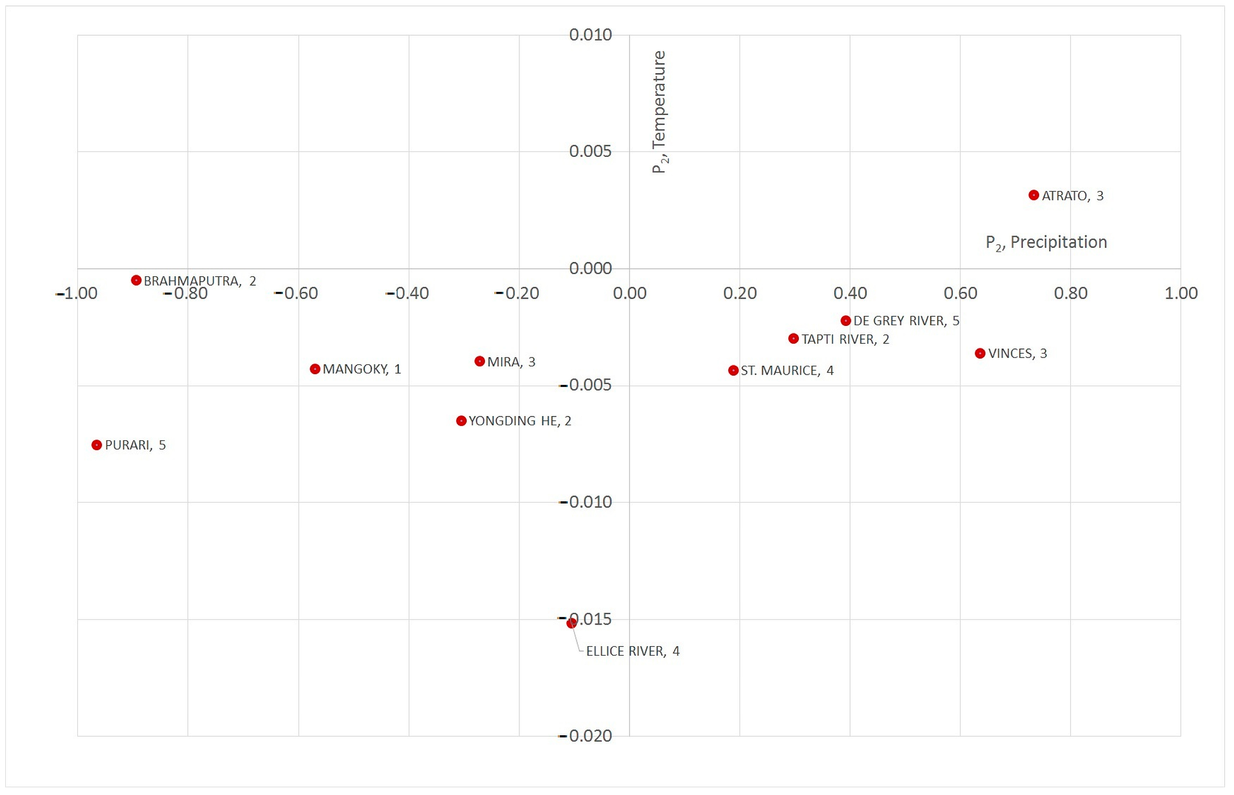
| Precipitation | Temperature | |||||||||
|---|---|---|---|---|---|---|---|---|---|---|
| No | WMO | River | Country | Area | tr (STD) | tr (RANGE) | P2 | tr (STD) | tr (RANGE) | P2 |
| mm/year | °C/year | |||||||||
| 15 | 1 | Mangoky | Madagascar | 53,225 | −0.2059 | −0.7757 | −0.5697 | −0.0018 | −0.0061 | −0.0043 |
| 45 | 2 | Yongding He | China | 42,500 | −0.0854 | −0.3907 | −0.3053 | −0.0050 | −0.0115 | −0.0065 |
| 75 | 2 | Brahmaputra | Bangladesh | 636,130 | −0.2147 | −1.1095 | −0.8948 | −0.0017 | −0.0022 | −0.0005 |
| 81 | 2 | Tapti River | India | 61,575 | 0.1281 | 0.4256 | 0.2975 | −0.0024 | −0.0054 | −0.0030 |
| 114 | 3 | Atrato | Colombia | 9432 | 0.3500 | 1.0835 | 0.7336 | 0.0014 | 0.0046 | 0.0032 |
| 168 | 3 | Mira | Ecuador | 4960 | −0.1104 | −0.3822 | −0.2719 | −0.0021 | −0.0060 | −0.0039 |
| 171 | 3 | Vinces | Ecuador | 4400 | 0.1595 | 0.7957 | 0.6361 | −0.0011 | −0.0047 | −0.0036 |
| 233 | 4 | Ellice River | Canada | 16,900 | −0.0433 | −0.1476 | −0.1043 | −0.0077 | −0.0228 | −0.0152 |
| 263 | 4 | St. Maurice | Canada | 42,000 | 0.0762 | 0.2647 | 0.1885 | −0.0052 | −0.0096 | −0.0043 |
| 295 | 5 | Purari | Papua New Guinea | 11,100 | −0.3654 | −1.3310 | −0.9656 | −0.0033 | −0.0108 | −0.0075 |
| 301 | 5 | De Grey River | Australia | 49,600 | 0.1442 | 0.5358 | 0.3916 | −0.0026 | −0.0048 | −0.0022 |
Disclaimer/Publisher’s Note: The statements, opinions and data contained in all publications are solely those of the individual author(s) and contributor(s) and not of MDPI and/or the editor(s). MDPI and/or the editor(s) disclaim responsibility for any injury to people or property resulting from any ideas, methods, instructions or products referred to in the content. |
© 2024 by the author. Licensee MDPI, Basel, Switzerland. This article is an open access article distributed under the terms and conditions of the Creative Commons Attribution (CC BY) license (https://creativecommons.org/licenses/by/4.0/).
Share and Cite
Twaróg, B. Assessing Polarisation of Climate Phenomena Based on Long-Term Precipitation and Temperature Sequences. Sustainability 2024, 16, 8311. https://doi.org/10.3390/su16198311
Twaróg B. Assessing Polarisation of Climate Phenomena Based on Long-Term Precipitation and Temperature Sequences. Sustainability. 2024; 16(19):8311. https://doi.org/10.3390/su16198311
Chicago/Turabian StyleTwaróg, Bernard. 2024. "Assessing Polarisation of Climate Phenomena Based on Long-Term Precipitation and Temperature Sequences" Sustainability 16, no. 19: 8311. https://doi.org/10.3390/su16198311
APA StyleTwaróg, B. (2024). Assessing Polarisation of Climate Phenomena Based on Long-Term Precipitation and Temperature Sequences. Sustainability, 16(19), 8311. https://doi.org/10.3390/su16198311