

Spatiotemporal Changes in Air Pollution within the Studied Road Segment


Abstract
1. Introduction
2. Justification of the Topic and Literature Review
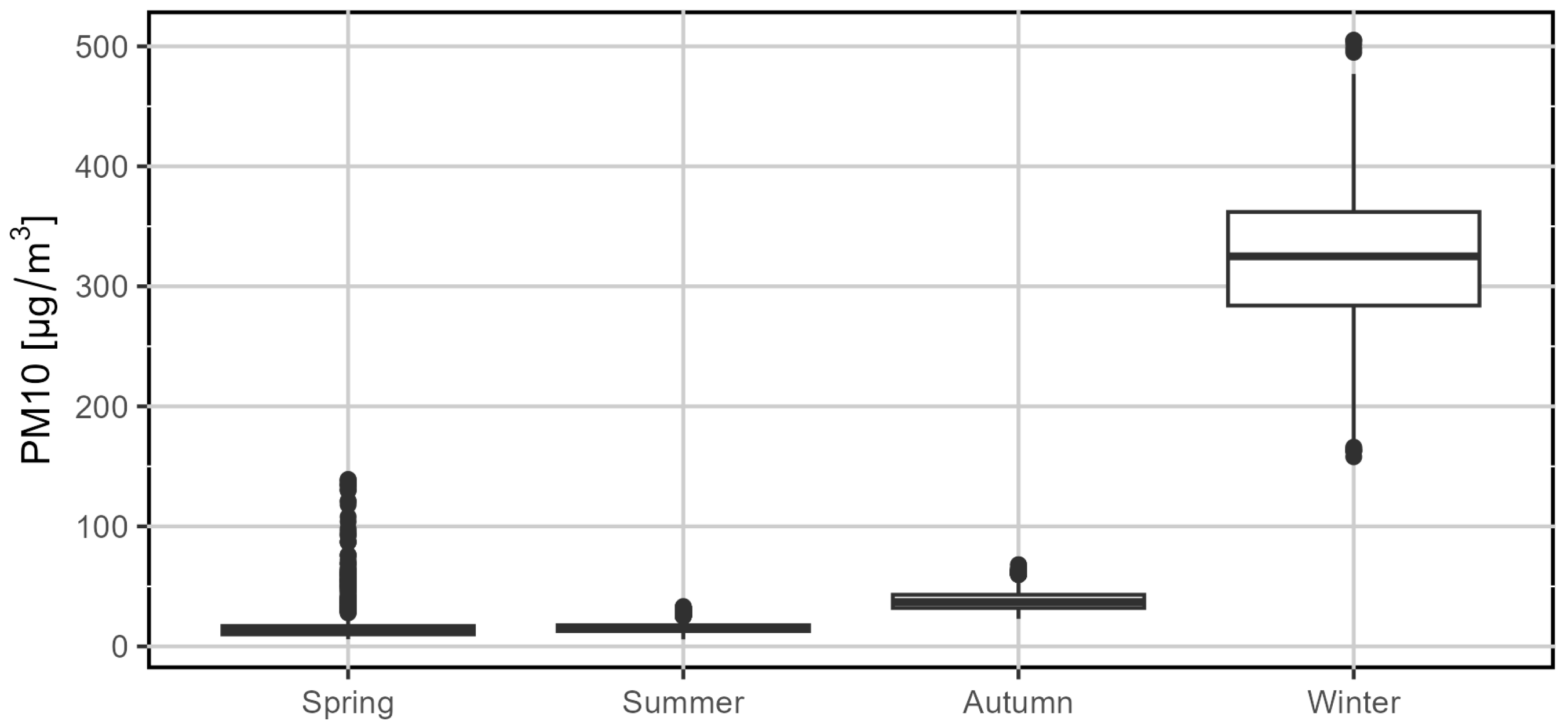
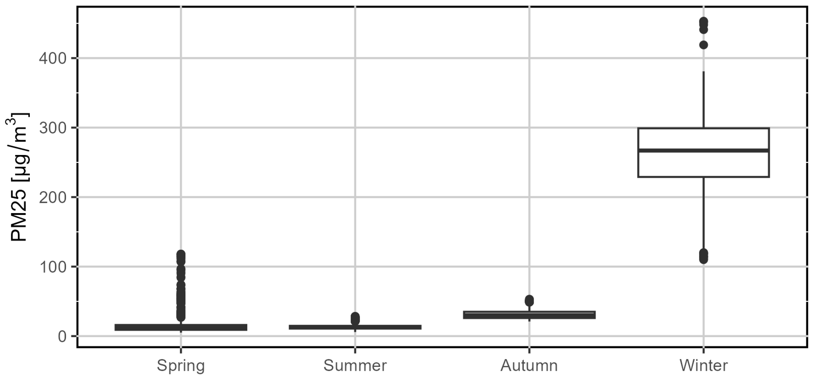
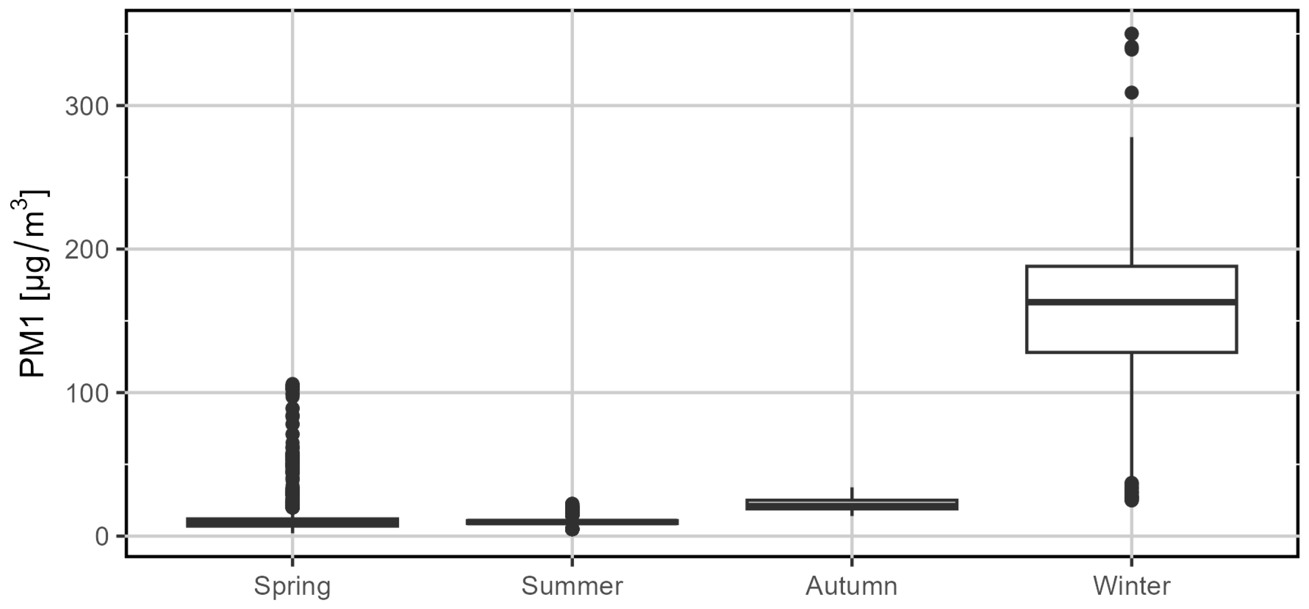
- Is there a significant difference in traffic pollutant emissions across the observed seasons (spring, summer, autumn, winter)?
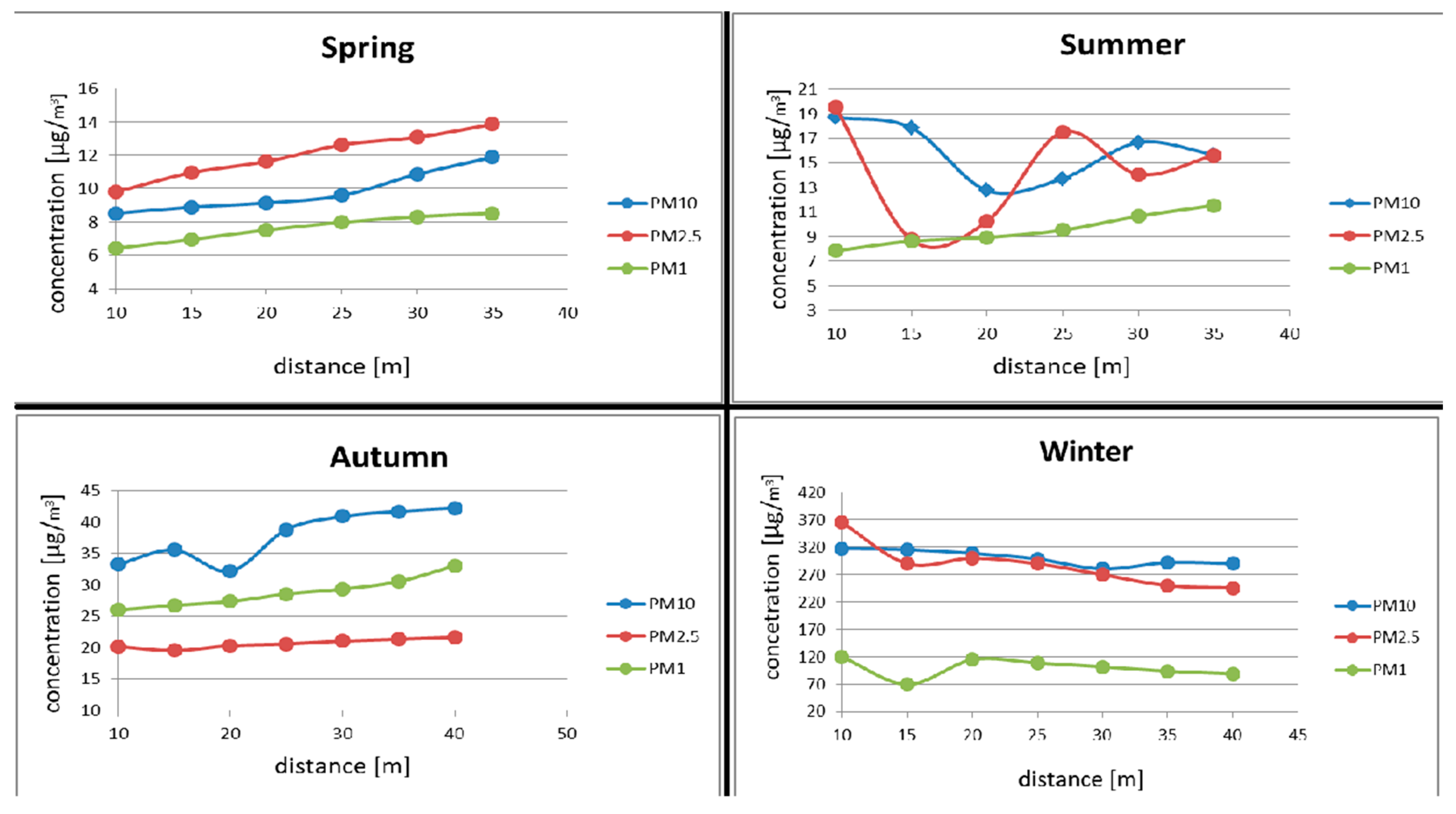
- Are there changes in the concentration of traffic pollutants with increasing distance from the road?
3. Materials, Methods and Results
- Checking the conformity of distributions with the normal distribution using the Lilliefors test.
- Determining whether the concentration distributions in different seasons differ using the Kruskal-Wallis test.
- Using the Wilcoxon test to identify specific concentration distributions that differ from each other.
- Employing Pearson’s correlation coefficient to check for a correlation between traffic pollutant concentration levels and distance from the road.
- Analyzing the significance of the obtained results.
- Drawing conclusions.
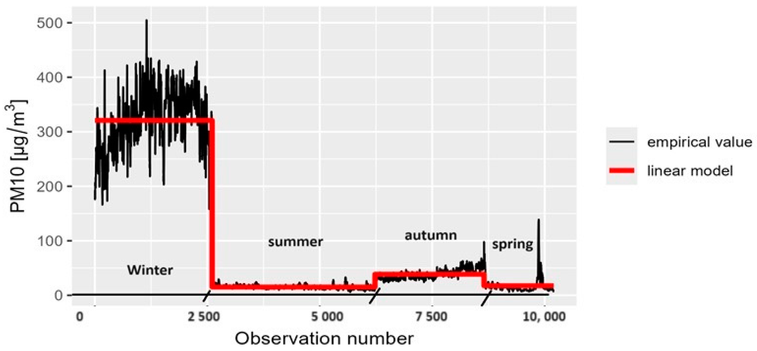
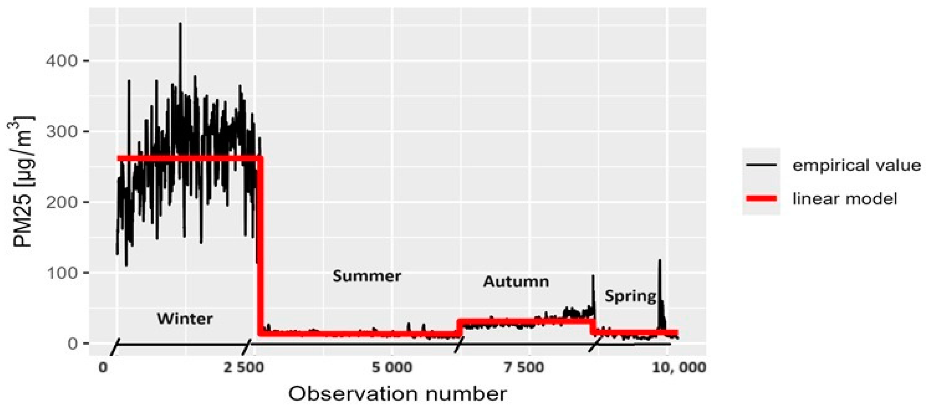
3.1. Checking Whether Traffic Pollutant Concentrations Differ by Season
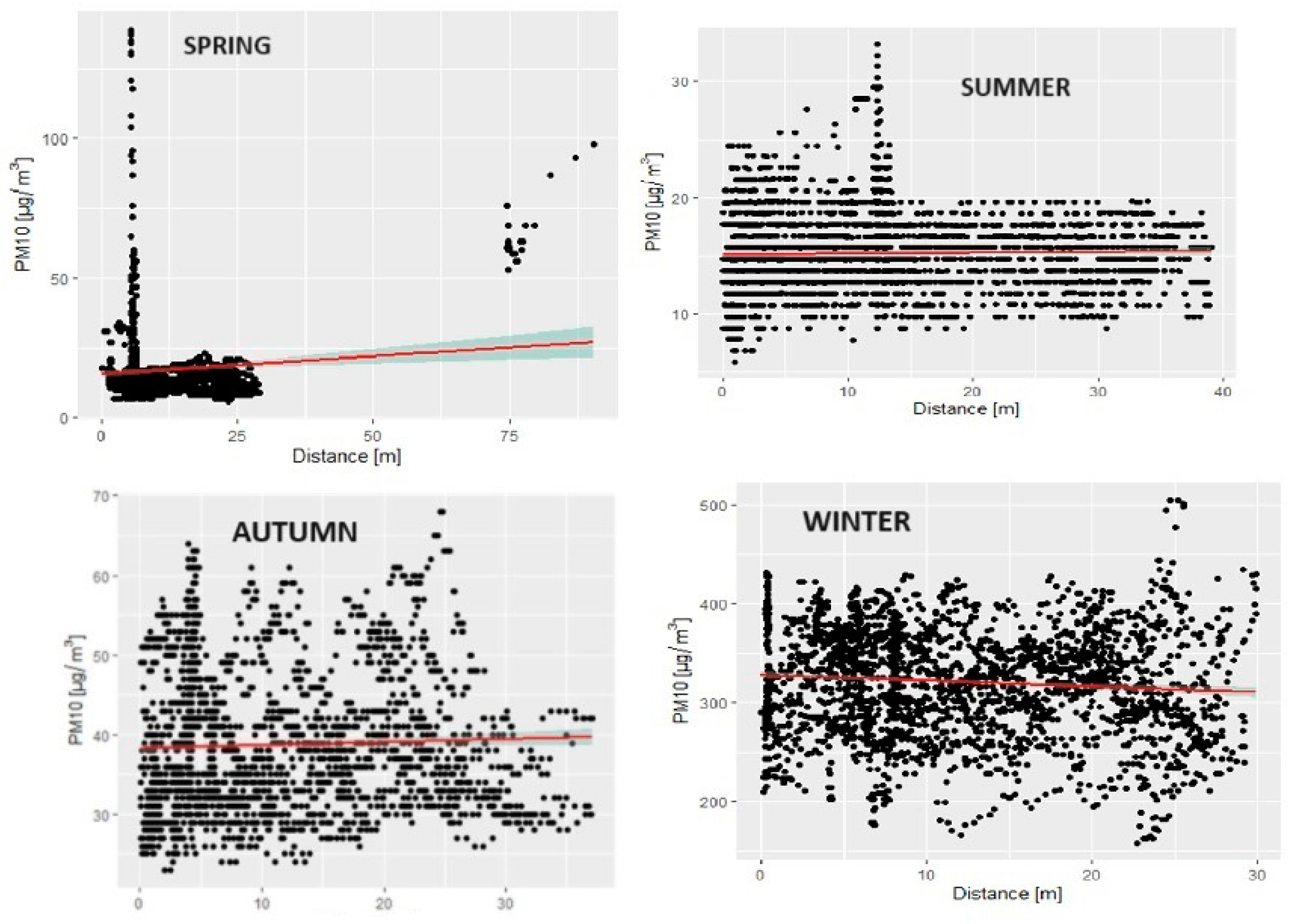
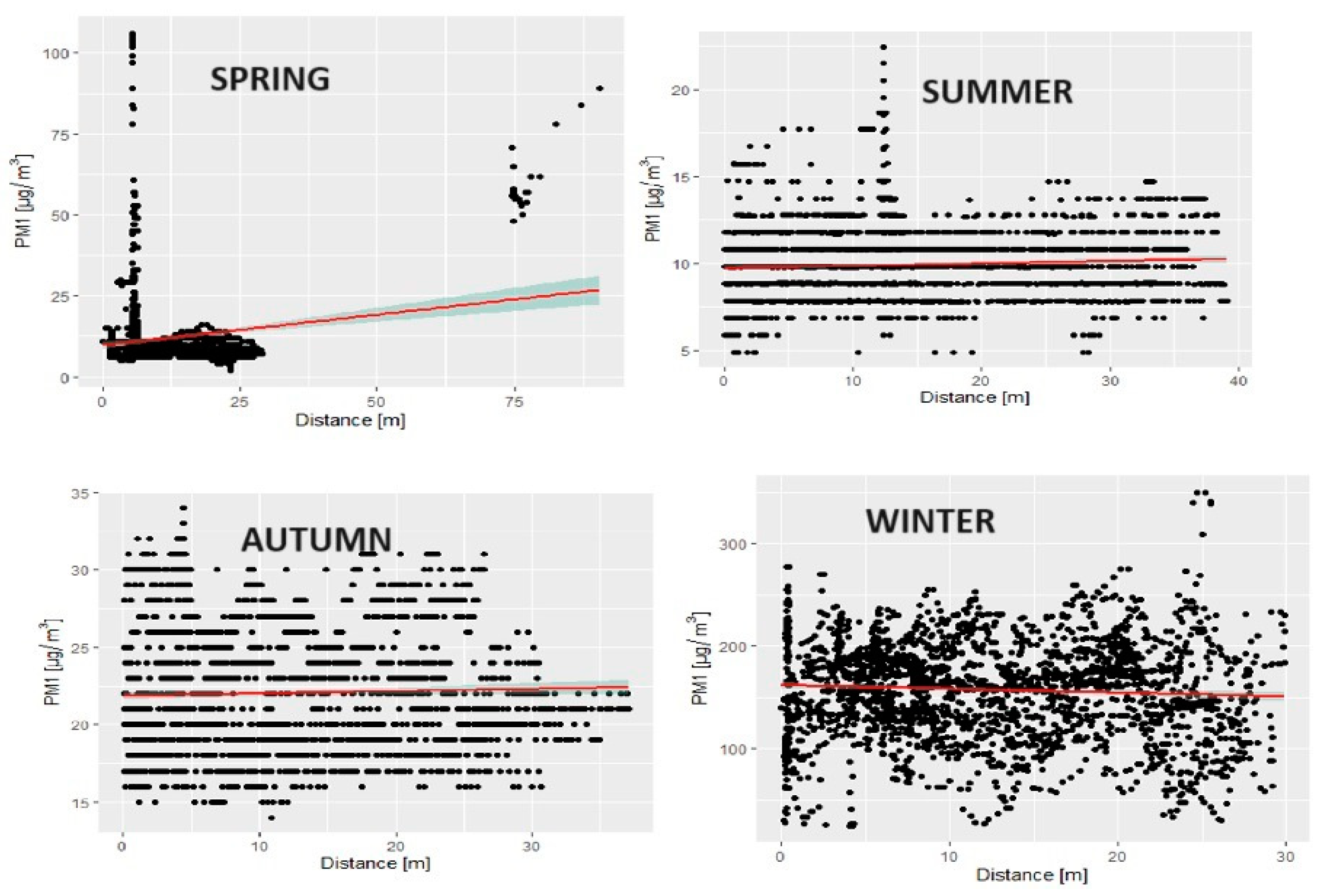
3.2. Determination of the Correlation between Traffic Pollutant Concentrations and the Distance from Their Source
4. Discussion of Results
Comparison of Measurement Results with Those of the Main Inspectorate of Environmental Protection
5. Conclusions
Author Contributions
Funding
Institutional Review Board Statement
Informed Consent Statement
Data Availability Statement
Conflicts of Interest
References
- Andrych-Zalewska, M.; Chłopek, Z.; Merkisz, J.; Pielecha, J. Research on the results of the WLTP procedure for a passenger vehicle. Eksploat. Niezawodn. Maint. Reliab. 2024, 26, 176112. [Google Scholar] [CrossRef]
- Sówka, M. Transport Drogowy jako źródło Zanieczyszczeń na Terenie Aglomeracji Miejskich/in English Road Transport as a Source of Pollution in Urban Agglomerations. 2017. Available online: https://www.researchgate.net/publication/312949957_Transport_drogowy_jako_zrodlo_zanieczyszczenia_powietrza_na_terenie_aglomeracji_miejskich_Road_transport_as_a_source_of_air_pollution_in_urban_agglomerations#fullTextFileContent (accessed on 24 June 2024).
- European Environment Agency (EEA). Available online: https://www.eea.europa.eu/en (accessed on 3 August 2023).
- Lei, Y.; Davies, G.M.; Jin, H.; Tian, G.; Kim, G. Scale-Dependent Effects of Urban Greenspace on Particulate Matter Air Pollution. Urban For. Urban Green 2021, 61, 127089. [Google Scholar] [CrossRef]
- Andrych-Zalewska, M.; Chlopek, Z.; Pielecha, J.; Merkisz, J. Investigation of exhaust emissions from the gasoline engine of a light duty vehicle in the Real Driving Emissions test. Eksploat. Niezawodn. Maint. Reliab. 2023, 25, 165880. [Google Scholar] [CrossRef]
- Maćkowiak, A.; Kostrzewski, M.; Bugała, A.; Chamier-Gliszczyński, N.; Bugała, D.; Jajczyk, J.; Nowak, K. Investigation into the Flow of Gas-Solids during Dry Dust Collectors Exploitation, as Applied in Domestic Energy Facilities—Numerical Analyses. Eksploat. Niezawodn. Maint. Reliab. 2023, 25, 174095. [Google Scholar] [CrossRef]
- Ghorani-Azam, A.; Riahi-Zanjani, B.; Balali-Mood, M. Effects of air pollution on human health and practical measures for prevention in Iran. J. Res. Med Sci. Off. J. Isfahan Univ. Med. Sci. 2016, 21, 65. [Google Scholar]
- Li, B.; Li, J.; Lu, J.; Xu, Z. Spatiotemporal Distribution Characteristics and Inventory Analysis of Near-Road Traffic Pollution in Urban Areas. Atmosphere 2024, 15, 417. [Google Scholar] [CrossRef]
- Lu, K.F.; He, H.D.; Wang, H.W.; Li, X.B.; Peng, Z.R. Characterizing temporal and vertical distribution patterns of traffic-emitted pollutants near an elevated expressway in urban residential areas. Build. Environ. 2020, 172, 106678. [Google Scholar] [CrossRef]
- Lu, W.; Howarth, A.T.; Adam, N.; Riffat, S.B. Modelling and measurement of airflow and aerosol particle distribution in a ventilated two-zone chamber. Build. Environ. 1996, 31, 417–423. [Google Scholar] [CrossRef]
- Hang, J.; Buccolieri, R.; Yang, X.; Yang, H.; Quarta, F.; Wang, B. Impact of indoor-outdoor temperature differences on dispersion of gaseous pollutant and particles in idealized street canyons with and without viaduct settings. Build. Simulat. 2018, 12, 285–297. [Google Scholar] [CrossRef]
- Cheo, Y.; Wang, Z.; Liu, C.; Peng, Z.R. Assessing neighborhood air pollution exposure and its relationship with the urban form. Build. Environ. 2019, 155, 15–24. [Google Scholar]
- Jin, J.; Sun, S.; Wang, F.; Ling, Y.; Wang, T.; Wu, L.; Wei, N.; Chang, J.; Mao, H. Vehicle Emission Inventory and Scenario Analysis in Liaoning from 2000 to 2020. Environ. Sci. 2020, 41, 665–673. [Google Scholar]
- Du, W.; Chen, L.; Wang, H.; Shan, Z.; Zhou, Z.; Li, W.; Wang, Y. Deciphering urban traffic impacts on air quality by deep learning and emission inventory. J. Environ. Sci. 2023, 124, 745–757. [Google Scholar] [CrossRef]
- Liu, Y.H.; Ma, J.L.; Li, L.; Lin, X.F.; Xu, W.J.; Ding, H. A high temporal-spatial vehicle emission inventory based on detailed hourly traffic data in a medium-sized city of China. Environ. Pollut. 2018, 236, 324–333. [Google Scholar] [CrossRef]
- Ghaffarpasand, O.; Talaie, M.R.; Ahmadikia, H.; Khozani, A.T.; Shalamzari, M.D. A high-resolution spatial and temporal on-road vehicle emission inventory in an Iranian metropolitan area, Isfahan, based on detailed hourly traffic data. Atmos. Pollut. Res. 2020, 11, 1598–1609. [Google Scholar] [CrossRef]
- Kumara, A.; Mishra, R.K.; Sarma, R. Mapping spatial distribution of traffic induced criteria pollutants and associated health risks using kriging interpolation tool in Delhi 2021. J. Transp. Health 2020, 18, 100879. [Google Scholar] [CrossRef]
- Jaroń, A.; Borucka, A.; Deliś, P.; Sekrecka, A. An Assessment of the Possibility of Using Unmanned Aerial Vehicles to Identify and Map Air Pollution from Infrastructure Emissions. Energies 2024, 17, 577. [Google Scholar] [CrossRef]
- Borucka, A.; Parczewski, R.; Kozłowski, E.; Świderski, A. Evaluation of air traffic in the context of the COVID-19 pandemic. Arch. Transp. 2022, 64, 45–57. [Google Scholar] [CrossRef]
- Komnos, D.; Tsiakmakis, S.; Pavlovic, J.; Ntziachristos, L.; Fontaras, G. Analysing the real-world fuel and energy consumption of conventional and electric cars in Europe. Energy Convers. Manag. 2022, 270, 116161. [Google Scholar] [CrossRef]
- Wang, Z.; Shangguan, W.; Peng, C.; Cai, B. Similarity Based Remaining Useful Life Prediction for Lithium-ion Battery under Small Sample Situation Based on Data Augmentation. Eksploat. Niezawodn. Maint. Reliab. 2024, 26, 175585. [Google Scholar] [CrossRef]
- Zhao, Z.; Xie, L.; Zhao, B.; Wang, L. Reliability assessment of folding wing system deployment performance considering failure correlation. Eksploat. Niezawodn. Maint. Reliab. 2024, 26, 175085. [Google Scholar] [CrossRef]
- Zheng, T.; Li, B.; Bing, X.; Zhanyong, L.; Li, S.; Ren, Z. Vertical and horizontal distributions of traffic-related pollutants beside an urban arterial road based on unmanned aerial vehicle observations. Build. Environ. 2021, 187, 107401. [Google Scholar] [CrossRef]


| Pollutant | Test Statistic Dn | p-Value | |
|---|---|---|---|
| Spring | PM10 | ||
| PM2.5 | |||
| PM1 | |||
| Summer | PM10 | ||
| PM2.5 | |||
| PM1 | |||
| Autumn | PM10 | ||
| PM2.5 | |||
| PM1 | |||
| Winter | PM10 | ||
| PM2.5 | |||
| PM1 |
| Pollutant | p-Value | |
|---|---|---|
| PM10 | 8352.1 | |
| PM2.5 | 8317.3 | |
| PM1 | 8257.9 |
| Autumn | Summer | Spring | ||
|---|---|---|---|---|
| PM10 | Summer | 0 | 0 | 0 |
| Spring | 0 | 0 | ||
| Winter | 0 | 0 | 0 | |
| PM2.5 | Summer | 0 | 0 | |
| Spring | 0 | 0 | ||
| Winter | 0 | 0 | 0 | |
| PM1 | Summer | 0 | 0 | |
| Spring | 0 | 0 | ||
| Winter | 0 | 0 | 0 |
| Pollutant | Correlation Coefficient | Test Statistic Value | p-Value | |
|---|---|---|---|---|
| PM10 | Spring | 0.0878 | 3.4665 | 0.0005 |
| Summer | 0.0188 | 1.1356 | 0.2562 | |
| Autumn | 0.0409 | 2.0159 | 0.0439 | |
| Winter | −0.0859 | −4.4006 | ||
| PM2.5 | Spring | 0.1379 | 5.4772 | |
| Summer | 0.0217 | 1.3046 | 0.1921 | |
| Autumn | 0.0349 | 1.7195 | 0.0856 | |
| Winter | −0.0884 | −4.5292 | ||
| PM1 | Spring | 0.1584 | 6.3101 | |
| Summer | 0.0541 | 3.2585 | 0.0011 | |
| Autumn | 0.0342 | 1.6844 | 0.0922 | |
| Winter | −0.0621 | −3.1777 | 0.0015 |
| Pollutant | UAV Data [μg/m3] | GIOŚ 1 Data [μg/m3] | GIOŚ 2 Data [μg/m3] | |
|---|---|---|---|---|
| PM10 | Spring | 17.48 | 29 | 21.8 |
| Summer | 15.94 | 15.6 | 12.3 | |
| Autumn | 38.67 | 84.5 | 21.1 | |
| Winter | 320.5 | 55.6 | 20.5 | |
| PM2.5 | Spring | 15.45 | 15.2 | 9.2 |
| Summer | 13.24 | 12.3 | 6.9 | |
| Autumn | 31.16 | 29.3 | 15.1 | |
| Winter | 262.04 | 25.0 | 15.9 | |
| PM1 | Spring | 12.41 | Not measured | Not measured |
| Summer | 9.85 | |||
| Autumn | 22.01 | |||
| Winter | 157.26 |
| Δ1 | Δ2 | ||
|---|---|---|---|
| PM10 | Spring | 65.91% | 24.83% |
| Summer | 2.13% | 21.15% | |
| Autumn | 118.52% | 75.03% | |
| Winter | 82.65% | 63.13% | |
| PM2.5 | Spring | 1.62% | 39.47% |
| Summer | 7.09% | 43.90% | |
| Autumn | 5.96% | 48.46% | |
| Winter | 90.45% | 36.40% |
Disclaimer/Publisher’s Note: The statements, opinions and data contained in all publications are solely those of the individual author(s) and contributor(s) and not of MDPI and/or the editor(s). MDPI and/or the editor(s) disclaim responsibility for any injury to people or property resulting from any ideas, methods, instructions or products referred to in the content. |
© 2024 by the authors. Licensee MDPI, Basel, Switzerland. This article is an open access article distributed under the terms and conditions of the Creative Commons Attribution (CC BY) license (https://creativecommons.org/licenses/by/4.0/).
Share and Cite
Jaroń, A.; Borucka, A. Spatiotemporal Changes in Air Pollution within the Studied Road Segment. Sustainability 2024, 16, 7292. https://doi.org/10.3390/su16177292
Jaroń A, Borucka A. Spatiotemporal Changes in Air Pollution within the Studied Road Segment. Sustainability. 2024; 16(17):7292. https://doi.org/10.3390/su16177292
Chicago/Turabian StyleJaroń, Agata, and Anna Borucka. 2024. "Spatiotemporal Changes in Air Pollution within the Studied Road Segment" Sustainability 16, no. 17: 7292. https://doi.org/10.3390/su16177292
APA StyleJaroń, A., & Borucka, A. (2024). Spatiotemporal Changes in Air Pollution within the Studied Road Segment. Sustainability, 16(17), 7292. https://doi.org/10.3390/su16177292