Abstract
Level of quality not only affects demand but also affects the proportion of imperfect products and then affects profit. This paper takes the quality level as a decision variable, considers both the consumer demand and the recovery of imperfect products in a dual-channel closed-loop supply chain (CLSC), and studies the significance of a revenue-sharing contract for coordination. The results show that the relationship between the optimal price and the quality level is affected by the repair cost of imperfect products and that the consumer’s attention to price and quality affects the trend of the overall profit with the quality level. In some cases, simply improving the quality level cannot expand the demand and is not even conducive to the improvement of green supply chain profits. It is also found that in both centralized and decentralized scenarios, coordination contracts can effectively motivate retailers to collect waste and help improve the economic efficiency of green supply chains.
1. Introduction
In a forward supply chain, manufacturers only sell products [1]. The closed-loop supply chain (CLSC) not only considers the production and sales of products but also considers the recycling and remanufacturing of waste products, which belong to the green supply chain [2,3]. More and more enterprises have established their own CLSCs, such as Apple, Huawei, Samsung, Dell, and Lenovo [4]. Apple announced a new recycling program in May 2014, which included all Apple products (previously, only certain models of iPhone were included) [2].
In a reverse supply chain, many enterprises recycle not only waste products but also imperfect products; for example, Huawei established a set of free electronic waste recycling mechanisms [5]. This behavior can increase customers’ trust, encourage customers to purchase products, and increase profits. When purchasing electronic products, customers will not only refer to the price [6] but also pay attention to the quality [7]. Therefore, product quality and pricing decisions play an important role in both the forward and reverse supply chains.
With the rapid development of the internet, many manufacturers sell products directly. For example, Huawei, Apple, HP, and Lenovo all distribute their products through direct (online) channels because they can attract and retain more loyal customers in this way [8,9].
With the emergence of network channels, scholars proposed the dual-channel CLSC, which means two channels (including a direct channel and an indirect channel) [10]. The dual-channel structure is beneficial to both manufacturers and retailers [11], and competition is generated. When choosing channels, consumers have preferences for online and offline channels and may also be influenced by factors such as channel price and service level [12]. This channel conflict intensifies the competition between manufacturers and retailers [13]. Therefore, in order to obtain the maximum profit from the supply chain, it is necessary to design a contract.
This paper considers product-quality decision making and designs a coordination contract to maximize the profit of dual-channel CLSCs. Our research attempts to address the following questions:
- (1)
- In the dual-channel CLSC competition model, considering quality demand, what is the impact of quality decisions about and maintenance costs of imperfect products on the pricing decisions and revenue of all parties?
- (2)
- Compared with the case without a coordination contract, does a revenue-sharing contract improve the overall profit of the supply chain?
- (3)
- When considering revenue, long-term development, and other issues, how should enterprises make decisions on product quality level, revenue-sharing rate, and other factors?
The innovations are as follows:
- (1)
- The endogenous variable of the product quality level is incorporated into a dual-channel CLSC, which not only considers the impact of quality level on cost and pricing but also considers the recovery of imperfect products caused by quality problems in reverse logistics, making the research more practical.
- (2)
- The impact of product quality on decision making is considered in both the forward supply chain and the reverse supply chain.
- (3)
- The impact of the coordination mechanism on supply chain decision making and the conflict between the two channels is considered.
The remainder of this paper is arranged as follows: Section 2 is a literature review. In Section 3, a model is proposed and assumptions are outlined. Section 4 shares results, and Section 5 discusses some properties. Section 6 is a numerical analysis and provides managerial insights. Finally, Section 7 concludes with a summary and suggestions for future research.
2. Literature Review
This paper is mainly related to four strands of the literature: dual-channel forward/closed-loop supply chains, price and quality competition in supply chains, product returns and recycling, and supply chain coordination.
2.1. Dual-Channel Forward/Closed-Loop Supply Chains
With the development of information technology, more and more consumers purchase products online, and enterprises establish dual-channel supply chains to attract customers [14]. For example, He et al. [15] proved that consumers’ free-riding behavior can also increase the profits of manufacturers. Giri et al. [13] studied the benefits of CLSCs dominated by different members. Taleizadeh et al. [7] compared the Stackelberg game model under the two situations of a single channel and dual channels. Xiao et al. [16] found that according to customers’ different levels of acceptance of online channels, traditional channels and dual channels can be the best choices for implementing a trade-in strategy. Rahmani et al. [14] analyzed the pricing of different channels and their impacts in the context of considering the green level of products. Wang et al. [17] designed a manufacturer to sell customized products online and studied the price differences between different products and different channels. Ma, C. M [18], based on government subsidies and demand disruptions, analyzed a closed-loop supply chain composed of a manufacturer and a retailer.
2.2. Price and Quality Competitions in a Supply Chain
Since the recognition of value-added services and the improvement of quality can increase consumers’ acceptance of online channels [8], many scholars have studied the price and quality competition in different channels.
In terms of pricing and service, Pi et al. [19] studied how decision makers compete in service and price when the demand of one channel is switched to other channels in the case of demand interruption. Parsaeifar et al. [20] established a three-level supply chain model with multiproduct competition with specific demand function. In order to find the best time for manufacturers and retailers to bargain over the wholesale price in a dual-channel supply chain, Matsui [21] proposed a game model with a vertical structure. Hosseini-Motlagh et al. [22] studied price competition among dealers in forward logistics and service competition in reverse logistics. Zhang et al. [23] studied the impact of low product quality returns in reverse logistics on vertical dual-channel management of a CLSC. Jabarzare and Rasti-Barzoki [24] considered a two-channel supply chain consisting of a manufacturer and a packaging company in which the manufacturer and the packaging company compete for price and quality decisions.
In terms of quality requirements, Hosseini-Motlagh et al. [25] found that product quality was closely related to the length of the warranty period. Li and Chen [26] studied the supply chain of two manufacturers supplying products of different quality to one retailer. Chakraborty et al. [27] showed that two manufacturers can increase profits by improving the difference between the two products in terms of quality (low-quality competition). However, they all compete for sales only through an offline channel. Ranjan and Jha [28] explored the pricing strategy among members of a dual-channel supply chain. Sarkar and Bhadouriya [29] discussed the manufacturer’s choice of green quality and the retailer’s price decision when the product’s green level exceeds a threshold. Lin et al. [30] found that under certain conditions, reducing product quality and wholesale price was beneficial to both manufacturers and retailers.
2.3. Return and Collection of Products
Regarding research on recycling, Modak et al. [31] considered three possible recycling channels: the retailer, the manufacturer and a third party. Wan and Hong [32] proved that both a remanufacturing subsidy and a recycling subsidy can improve the recycling rate and the profit. Xing et al. [33] showed that the degree of competition of third-party recyclers is negatively correlated with the expected utility of manufacturers and third-party recyclers. However, none of the above literature references considers the quality level of recycled products (imperfect products/waste products). Although the model proposed by Almaraj and Trafalis [34] is applicable to the recycling problem of products that can be reused as raw materials (defective products/discarded products), they only considered the production of imperfect-quality products under multiple uncertainties. Taleizadeh and Moshtagh [35] found that the quality level of new products is different from that of remanufactured products. Khara et al. [36] proposed a CLSC production inventory model and that included sequential optimization. Huang M et al. [37] studied retailers and third parties competing to collect used products, along with CLSC pricing decisions and recycling strategies. Jian, J. et al. [38] proposed that in order to maximize profits, the optimal choice for all parties in the supply chain is to choose an alliance. Zeng and Hou [39] compared two different incentive strategies for recycling enterprises and suppliers with a large number of used mobile phones.
2.4. Supply Chain Coordination Contracts
A contract is an important means of coordination. He [40] analyzed different types of supply risk-sharing contracts. Hosseini-Motlagh et al. [22] proposed a wholesale price contract based on multilateral compensation. Xu et al. [41] designed an online channel price discount contract and an offline channel price discount contract to coordinate the supply chain and determined the coordination effect between the two kinds of price discount contracts. Ranjan and Jha [28] realized channel coordination among members of the supply chain through a residual profit sharing contract. Fan et al. [42] established the same quality-improvement cost-sharing contract, which proved that it could effectively coordinate the supply chain under manufacturer-led and retailer-led conditions. Wang Y et al. [43], based on the ‘effort cost sharing contract’, analyzed the effect of the contract on the supply chain profit.
In terms of revenue-sharing contracts, Xie et al. [12] analyzed the effect of revenue sharing according to the characteristics of recovery rate fluctuations. Wu et al. [44] constructed a revenue-sharing contract between a recycling center and a TPR. Zhang et al. [23] proposed a revenue-sharing contract to encourage retailers to recycle waste products. Jabarzare and Rasti-Barzoki [24] found that when customer demand is highly sensitive to product quality, contracts are more beneficial to cooperation. Zhu et al. [45] proposed a joint contract comprising a revenue-sharing contract and a repurchasing contract. Although Xing et al. [33] believed that the revenue-sharing contract had almost no impact on the manufacturer’s profit, it can be found from the above studies that the contract can indeed effectively coordinate the players in the supply chain and play a role in alleviating channel conflicts and increasing supply chain profits.
2.5. Research Gaps and Contributions
Regarding the existing literature, the following research gaps are found:
(1) When considering the impact of product-quality decision making on a CLSC, few studies have considered the impact of quality level on both the demand of the forward supply chain and the recovery rate of the reverse supply chain. Xie et al. [46] focused on the recycling of low-quality products but did not take into account the demand for product quality in the positive supply chain. (2) Most of the literature only considers waste recycling in the reverse supply chain, but in reality, the return rate of imperfect products will also have an impact on supply chain revenue; for example, Jabarzare and Rasti-Barzoki [24] considered that manufacturers and packaging companies compete in product sales price and quality decisions, but they did not include the return of imperfect products in their study.
In order to address these gaps, we establish a dual-channel CLSC that considers both waste recycling and imperfect product recycling, and we discuss the impact of product quality on the optimal pricing, the revenue of all parties, and the overall revenue in competition. At the same time, we design a revenue-sharing contract to coordinate the benefits of all parties in the supply chain.
Some of the relevant literature research is shown in Table 1.

Table 1.
Comparison between our paper and the related literature.
3. Model and Assumptions
3.1. Problem Statement
As shown in Figure 1, this paper considers a two-stage CLSC consisting of one manufacturer and one retailer. In forward logistics, retailers sell products offline while manufacturers also sell their products online. Our study also considers the recycling of imperfect products and waste products in reverse logistics. Waste products increase corporate income through remanufacturing, and imperfect products are recycled and returned to consumers after repair. The relationship between the manufacturer and the retailer is a Stackelberg game, in which the manufacturer is the leader and the retailer is the follower.
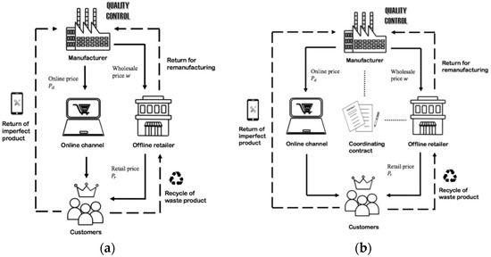
Figure 1.
Closed-loop supply chain structure. (a) CLSC without coordination contract; (b) CLSC with coordination contract.
The parameters and decision variables are shown in Table 2.

Table 2.
Parameters and decision variables.
3.2. Assumptions
In order to determine the model, some basic assumptions are put forward here.
Assumption 1.
The market demand is linearly related to price and quality level, which is widely used in such studies [47,48].
Assumption 2.
The quality of products sold in the offline channel is the same as that in the online channel, and the manufacturer’s wholesale price is lower than the online price, < .
Assumption 3.
There is a linear relationship between the manufacturing cost per unit of a new product and the quality level, , where is the sensitivity coefficient of production cost of a new product to quality. For imperfect products, the manufacturer needs to incur maintenance costs, .
Assumption 4.
Usually, the higher the quality of products, the lower the proportion of imperfect products and the lower the recycling rate. There is also a threshold at which consumers can tolerate low quality. Similar to the literature by Zhang et al. [23], we establish a recovery rate function that considers consumers’ tolerance for low-quality products: , where represents the effective coefficient that the recovery rate is affected by the quality of product, and represents the maximum tolerance of consumers when . Each imperfect product is returned only once.
Assumption 5.
In order to motivate the retailer to recycle the waste products, the manufacturer distributes part of its own revenue to the retailer according to the revenue-sharing rate stipulated in the coordination contract. As in Zhang et al. [23], by referring to Xing et al. [50], , where denotes the recycling efforts, denotes the recycling efforts’ sensitivity to revenue-sharing rate, and denotes the sensitivity of recycling rate to retailers’ recycling efforts.
3.3. Model
3.3.1. Without Coordination Contract
- (1)
- Decentralized decision scenario.
As the leader of the game, the manufacturer decides the online price, the wholesale price. and the quality level of the product. The manufacturer’s profit comes from the production of new products and the recycling and remanufacturing of waste products. According to the previous section, a defective product will be directly returned to the consumer free of charge after repair, which will generate certain costs for the manufacturer. In the case of no coordination mechanism, the value of the revenue-sharing rate = 0, . The profit is as follows:
- (2)
- Centralized decision scenario.
Under a centralized decision scenario, all members act with the objective of maximizing the overall profit. Combining Equations (3) and (4), the overall profit function can be obtained:
3.3.2. With Coordination Contract
- (1)
- Decentralized decision scenario.
In order to encourage retailers’ recycling efforts, manufacturers share part of their profits with retailers. Similar to Xie et al. [12], the profit function is as follows:
Only when will the manufacturer and the retailer be willing to enforce the contract.
- (2)
- Centralized decision scenario.
Similar to Section 3.3.1, in the case of a centralized decision scenario, all members focus on the maximum overall profit. Combining Equations (6) and (7), the overall profit can be obtained:
4. Results
For the above four scenarios, the backward induction method is used to solve them, respectively, and the results are shown in the Table 3 and Table 4. In order to make the expression more concise and clear, the expression – is listed in Appendix A, and the calculation and proof process is detailed in Appendix B. The overall profit of the supply chain is listed in Appendix C, as the expression is too complex.

Table 3.
Results without coordination contract.

Table 4.
Results with coordination contract.
5. Discussion
In this section, we conduct a qualitative analysis based on the result.
Property 1.
The relationship between the optimal pricing and the quality level is uncertain, and its trend is affected by the maintenance cost of an imperfect product, dual-channel quality sensitivity coefficient, price sensitivity coefficient, cross-price sensitivity coefficient, and other factors. When the maintenance cost is lower than the threshold /, the optimal retail price/online price increases with the quality level; otherwise, it decreases with the quality level. Similarly, this relationship is also applicable to the optimal online price.
Proof.
Taking the first derivative of , with respect to , we can obtain
□
Property 2.
The growth rates of the retail price and online price with regard to revenue-sharing rate
are the same, both of which are . As increases, both the retail price and online price decrease.
Proof.
Taking the first derivatives of and with regard to , respectively, we can obtain
□
Property 3.
With the increase in preference for offline channels, the optimal retail price increases, while the optimal online price decreases. As consumers’ preference for offline channels decreases, the optimal offline channel product price decreases and the optimal online channel product price increases.
Proof.
Taking the first derivatives of and with regard to , respectively, we can obtain
□
Property 4.
The relationship between the optimal online price and retail price is uncertain, which is related to the sensitivity of consumers to price and quality.
Proof.
Assume that .
1. If :
(1) when .
(2) when .
2. If :
(1) when .
(2) when .
□
Property 5.
Under the decentralized decision scenario, the impact of coordination contracts on retail prices is uncertain, while under the centralized decision scenario, the retail price without coordination is always greater than that with coordination.
Proof.
where , . Assume that .
1. If :
(1) If , , then .
(2) If , : when ; when .
2. If :
(1) If , : when ; when .
(2) If , , then .
□
Property 6.
In both the decentralized and centralized decision scenarios, the online price without coordination is higher than that with coordination.
Proof.
□
Property 7.
The relationship between the overall profit and the quality level is not clear. It is related to consumers’ sensitivities to price and quality level and the threshold value of quality level .
Proof.
Taking the first derivative of Equation (8) with regard to , we can obtain
where , . Assume that .
1. If :
(1) If , , then , and the overall profit increases with the improvement in quality.
(2) If , : when , then the overall profit increases with the improvement in quality; when , then the overall profit decreases with the improvement in quality.
2. If :
(1) If , : when , then the overall profit declines with the improvement in quality; when , then the overall profit increases with the improvement in quality.
(2) If , , then , and the overall profit decreases with the improvement in quality.
□
Property 8.
The relationship between the overall profit and the revenue-sharing rate is also uncertain, which depends on the cross-price sensitivity and the threshold of the revenue-sharing rate .
Proof.
Taking the first derivative of Equation (8) with regard to , we can obtain
where .
1. If , , then , and the overall profit increases with the increase in the revenue-sharing rate.
2. If , :
(1) If , then . The overall profit increases with the increase in the revenue-sharing rate.
(2) If , when , then the overall profit increases with the increase in the revenue-sharing rate; when , then the overall profit decreases with the increase in the revenue-sharing rate.
□
6. Numerical Analysis and Managerial Insights
6.1. Numerical Analysis
6.1.1. Value Analysis of the Centralized CLSC with Coordination
Without loss of generality, in order to demonstrate the properties above and reflect the differences in the pricing decisions and the overall profits among different models, we set the parameter values according to the production practice of an electronics enterprise in Zhejiang, China: , , , , , , , , , , t , , , , , and all of them need to satisfy the constraints proposed in Section 3.
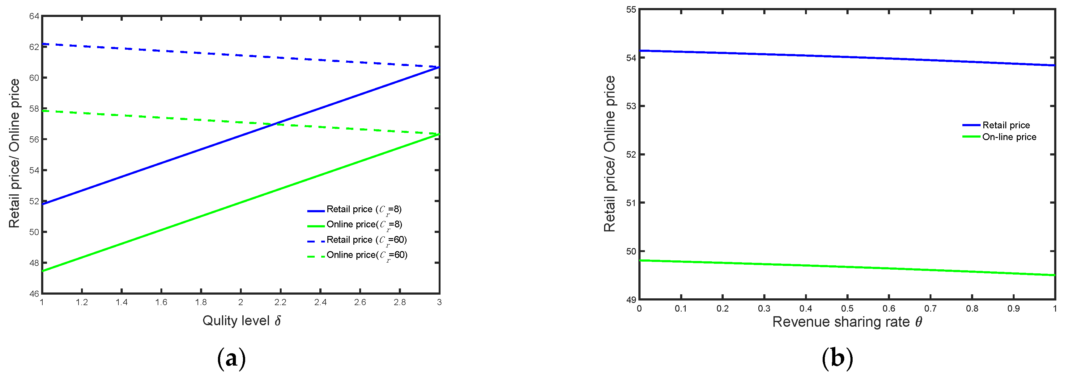
Figure 2a shows the relationship between the optimal online/retail price and product quality level, which verifies Property 1. When the maintenance cost is lower than the threshold (), the optimal retail price increases with the improvement in quality level; when the maintenance cost is higher than the threshold (), it decreases as the quality level increases.
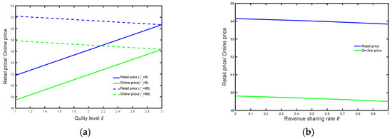
Figure 2.
Optimal online price/retail price. (a) Optimal online price/retail price and product quality level; (b) optimal online price/retail price and revenue-sharing rate.
Figure 2b shows the relationship between the optimal retail/online price and the revenue-sharing rate , which verifies Property 2. The growth rate of the online price and retail price on the revenue-sharing ratio is the same, so the trend is two parallel curves. With the increase in the revenue-sharing ratio, both the online price and the retail price decrease. The reason for this phenomenon is that with the increase in the revenue-sharing ratio, the sales competition between offline stores and online stores will become more intense, and the two sides have to reduce the price to obtain a larger consumer market.
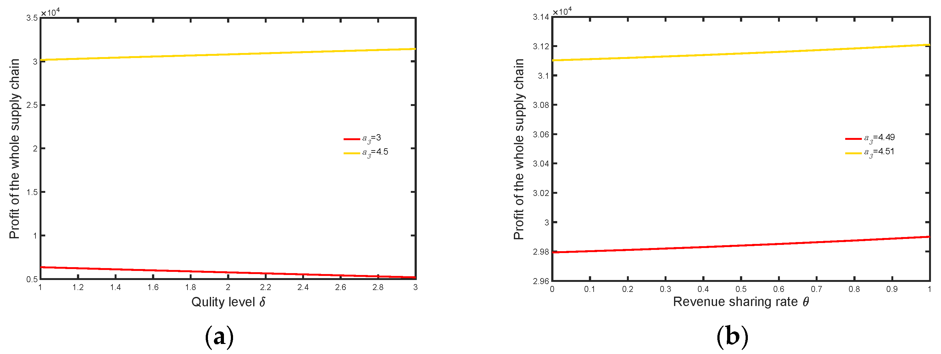
According to Property 7 and Property 8, the relationship between the optimal overall profit and the quality level/revenue-sharing rate is uncertain. Owing to that, there are too many cases of discussion, some of which are not constrained by the conditions in the hypothesis, so only typical cases are analyzed numerically here.
Figure 3a shows the relationship between the optimal overall profit and the quality level. Keep the values of other parameters unchanged. Set , and in this case, , is less than the threshold , and the overall profit increases with the increase in quality level; set , and in this case, , , and the overall profit decreases with the increase in quality level, which verifies the correctness of Property 7.
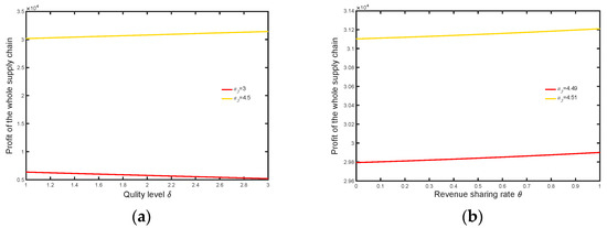
Figure 3.
Optimal overall profit. (a) Optimal overall profit and product quality level; (b) optimal overall profit and revenue-sharing rate.
Figure 3b validates Property 8. When the cross-price sensitivity coefficient of products is low (), the condition is met, and the overall profit increases with the increase in revenue-sharing rate. When the cross-price sensitivity coefficient of the product is high (), the overall profit increases monotonically with the increase in the revenue-sharing rate. However, it cannot be assumed that the total profit of the supply chain can be increased simply by increasing the revenue-sharing rate. Property 8 also shows that when the threshold is exceeded, the overall profit decreases monotonically with the increase in the revenue-sharing rate. Similar to Xie et al. [12], blindly increasing the revenue-sharing rate will reduce the manufacturer’s willingness to participate in coordination, which is detrimental to the overall profit.
6.1.2. Comparison of the Price
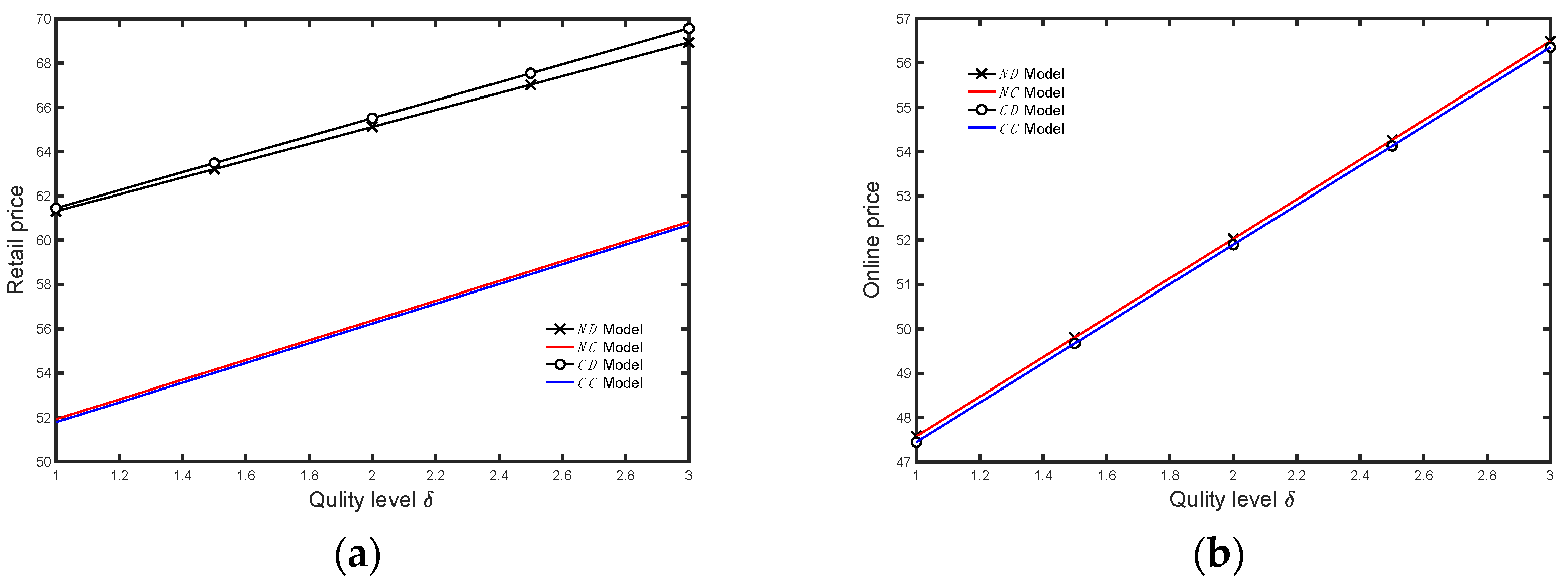
Figure 4a demonstrates that the retail price increases monotonically with the increase in quality level in all models. According to Property 5, in the decentralized scenario, if the conditions and are satisfied and is always below the threshold , then the retail price without coordination is less than that with coordination. However, in the centralized scenario, the retail price without coordination is always higher than that with coordination. This may be because the revenue-sharing contract can play a role in reconciliation under a centralized scenario, and both sides of the game are willing to jointly reduce the retail price to attract more potential consumers and maximize the overall profit.
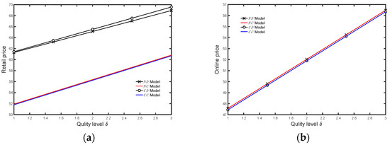
Figure 4.
Optimal retail/online price. (a) Optimal retail price and product quality level. (b) Optimal online prices and product quality levels.
Figure 4b shows the trend of the optimal online price with regard to quality level in four models. In all models, the online price increases monotonically as the quality level increases. This illustrates that the transition from a decentralized to a centralized mode will not drive the manufacturer to change the online price. Since the retailer does not interfere directly with the setting of the online price, the manufacturer can keep the original online market by keeping the online price unchanged. We also find that the online prices in CD and CC models are always lower than in ND and NC models, indicating that the existence of a coordination mechanism enables the manufacturer to reduce the online price.
We also provide four sets of numerical parameters that show the difference in overall supply chain profits under different model structures (i.e., , , , and models). Parameter settings are shown in Table 5.

Table 5.
Four numerical example datasets.
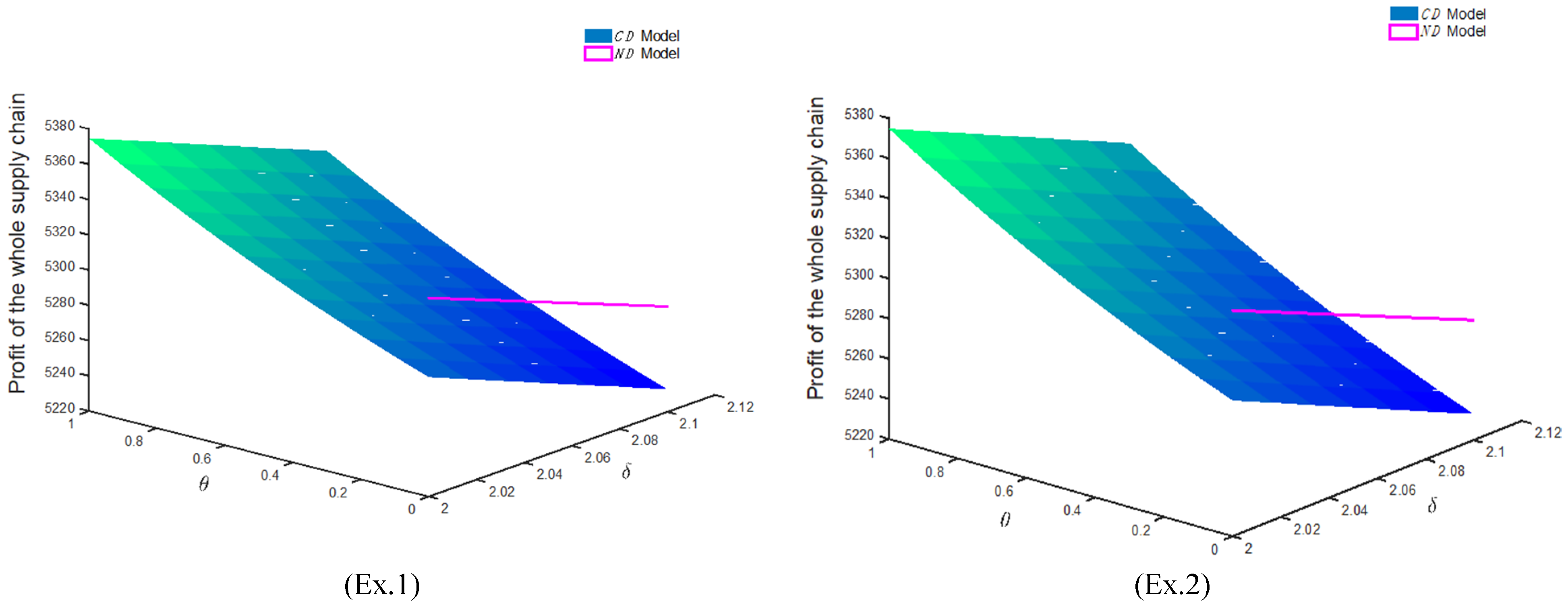
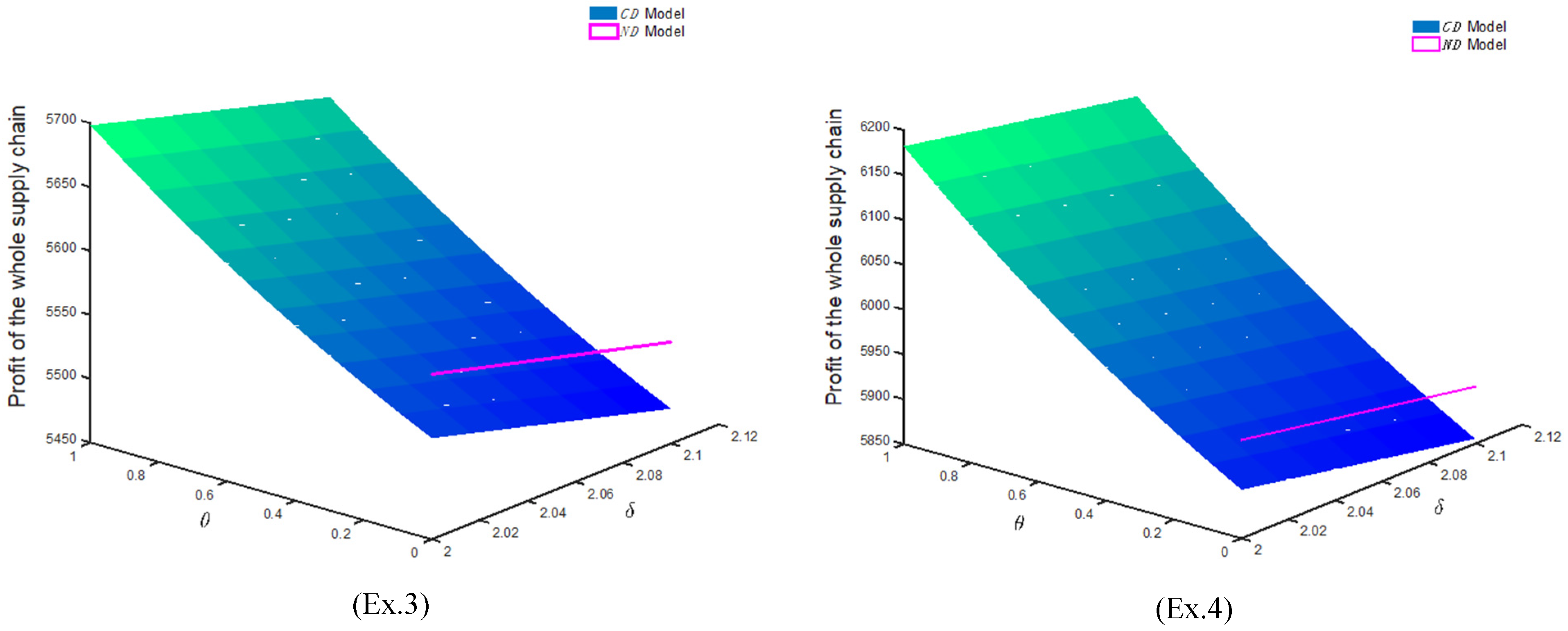
Figure 5 shows the comparison between the overall profit with coordination ( model) and that without coordination ( model) in a decentralized situation. In the model, the overall profit is displayed as a straight line rather than a curved surface, which is caused by the fact that the manufacturer does not share their revenue with the retailer (i.e., ). From Figure 5, we find that when the revenue-sharing rate is 0, the overall profit in the model is higher than that in the model. However, as increases, the profit of the SC with coordination gradually exceeds that without coordination, and the growth rate also rises. This demonstrates that under the coordination mechanism, it is possible that the manufacturer and the retailer reach a partnership and improve the overall profit by jointly setting a reasonable revenue-sharing rate even though they are in a decentralized scenario. This phenomenon can be seen in all four parameter examples, which reveals the effectiveness and stability of the coordination mechanism.
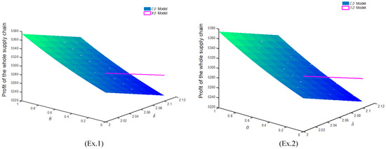

Figure 5.
Comparison of overall profit of model and model.
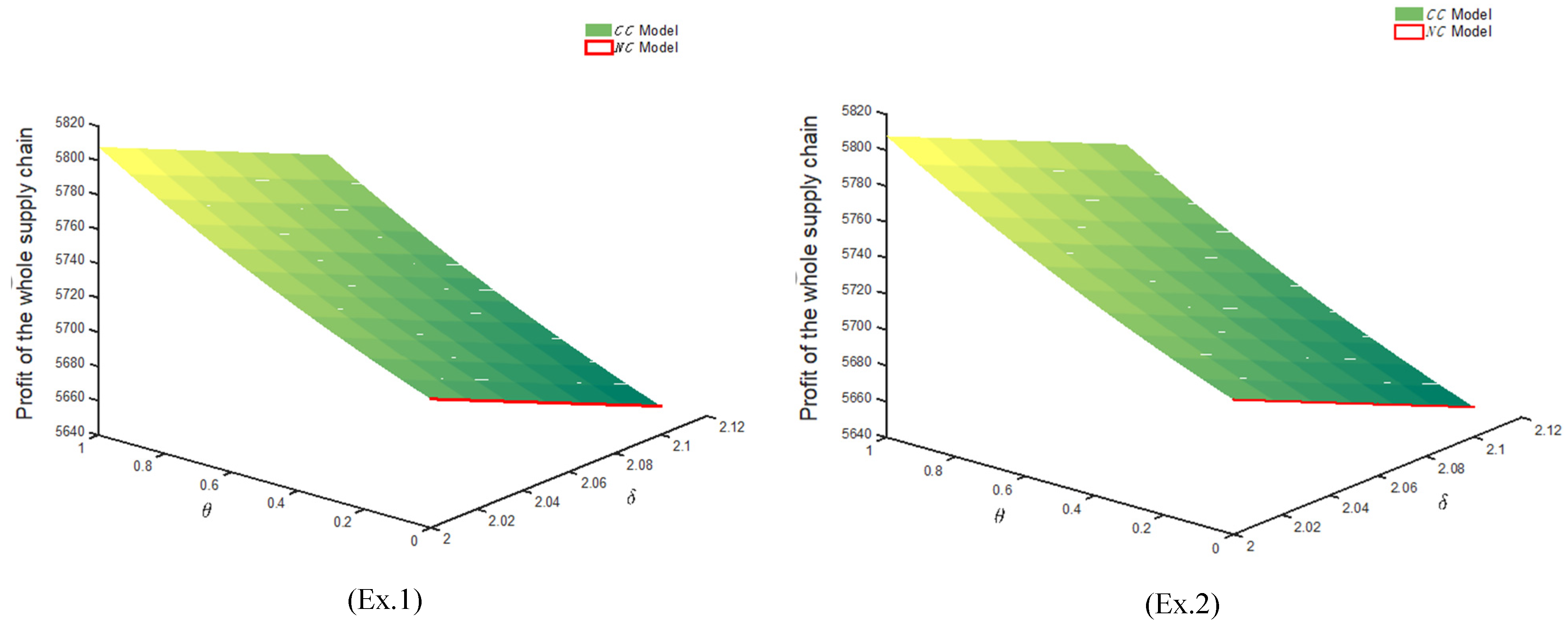
In the centralized scenario, the overall profits with coordination ( model) and that without coordination ( model) are showed in Figure 6. Similar to Figure 5, the model is displayed as a curved surface, and we find that the overall profit is always higher than that in the model regardless of how the product quality level and the revenue-sharing rate change. This comparison demonstrates that the manufacturer can successfully stimulate the retailer to collect waste products after the manufacturer shares their revenue. This behavior is beneficial to both of them, and the coordination mechanism can effectively help them to achieve the goal of maximizing the overall profit. Furthermore, it can be seen from different examples that no matter how the exogenous variables change, this conclusion always holds, which proves the significance of the existence of a coordination mechanism again.
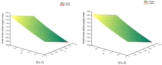
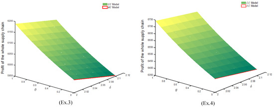
Figure 6.
Comparison of overall profit of model and model.
6.2. Managerial Insights
From the above analysis, we can obtain the following management insights:
- (1)
- According to Property 4,manufacturers and retailers should take a serious look at the importance that consumers place on price and quality. When consumers pay more attention to the price, the quality demand will be less important. According to the analysis of Property 5 and Property 6, under the coordination mechanism, manufacturers can take advantage of this information to sell low-quality products through online channels to gain profits. At this time, retailers should make full use of the low-price characteristic to expand their offline market and make great efforts to collect waste products to maximize benefits. While some consumers pursue product quality more, if the enterprises still sell inferior products through the online channel, they will lose social recognition and damage their brand reputation. Thus, manufacturers should produce high-quality products to regain the reputation of their enterprises, while retailers are better off reducing the retail price in order to increase their competitiveness and avoid the shrinkage of the retail market.
- (2)
- Manufacturers should not blindly pursue high-quality products to enter the high-end market. According to Property 7 and the numerical analysis in Figure 5, when including consumers’ demand for quality, we find that simply improving the quality level cannot directly expand the demand and increase profits and even is detrimental to the improvement of the overall profits. The quality level affects the production cost and the rate of imperfect products. According to Property 1, it is a better direction for enterprises to find ways to reduce the repair cost if they position their brands at a low level. To avoid large-scale inefficient investments, manufacturers should control the product quality in a specific range and generate additional benefits by remanufacturing. However, the recycling of waste products is largely influenced by retailers’ collecting efforts. For the sake of enlarging the remanufacturing market, it is especially important to stimulate retailers to collect waste products.
- (3)
- According to the numerical analysis in Figure 5 and Figure 6, manufacturers and retailers should reasonably set the revenue-sharing rate. According to Property 8, the relationship between the overall profit of the supply chain and the revenue-sharing ratio is not clear, which is also reflected in the numerical analysis in Figure 6. The coordination mechanism can encourage retailers to participate in remanufacturing activities and increase their recycling efforts. From the above analysis, we can find that the contract can not only alleviate channel conflict and weaken the double marginalization but also greatly improve the overall profits. Nevertheless, blindly increasing the revenue-sharing rate will make both the online and retail prices distort downwards. Hence, manufacturers and retailers should jointly formulate the right revenue-sharing rate to increase their own revenues.
7. Conclusions
The development of the internet and the improvement of people’s environmental awareness promote the development of dual-channel CLSCs. Based on the channel structure consisting of a single manufacturer and a single retailer under centralized and decentralized scenarios, we establish a joint optimization model considering pricing, product quality, return of imperfect products, and coordination. Specifically, we suppose that consumer’s demand depends on the price and quality level; the probability of consumers returning imperfect products relies on the initial quality level, and the recycling rate of waste products is related to the retailer’s collecting efforts. As the emergence of online channels leads to channel conflicts, a coordination mechanism is designed to ease the friction between the manufacturer and the retailer and improve the overall profits. We construct four models and discuss the influences of quality level and coordination contracts on the retail/online price and the overall profits, respectively, then we compare the results of different models. Furthermore, we verify the proposed properties by numerical analysis. Finally, we give some management insights and suggestions for enterprises.
The findings of this paper include the following:
- (1)
- The relationship between optimal retail/online price and quality is uncertain. When the maintenance cost is low, the optimal retail/online price increases with the product quality level and decreases otherwise. In addition, similar to the research conclusion of Zhang et al. (2020) [23], the growth rate of retail and online prices is the same, and both decrease with the increase in the revenue-sharing rate, so consumer surplus increases.
- (2)
- The trend of the optimal overall profit of the supply chain with quality will be affected by the consumer’s attention to price/quality and the threshold of quality level. In addition, the relationship between the optimal overall profit of the supply chain and the revenue-sharing rate is also uncertain, which is related to the consumer’s sensitivity to price and the threshold of the revenue-sharing rate.
- (3)
- The contract can play a mediating role and alleviate channel conflicts. Both sides of the game are willing to reduce the retail price to attract more potential consumers and maximize the overall profit of the supply chain. A coordination mechanism can help a supply chain increase its overall profit. In the decentralized case, with the increase in the revenue-sharing rate, the overall profit of the supply chain with a coordination contract gradually exceeds that without a coordination contract, and the growth rate increases slowly. Under centralized decision making, no matter how the revenue-sharing rate changes, the overall profit of the supply chain with coordination contracts is always higher than that without coordination contracts.
There are still some limitations in this paper. Firstly, future research could consider stochastic demand functions for product quality instead of linear demand functions. Secondly, it may be more realistic to include the recycling cost of used products in the model. Finally, this paper only considers a single manufacturer and retailer, and the competition between multiple manufacturers or retailers can be pursued in further research. These future works may add to the practical implications of remanufacturing.
Author Contributions
D.F.: project administration, funding acquisition; Y.M.: conceptualization, writing—review and editing; S.L.: methodology, investigation, Writing—original draft; Y.Z.: supervision, validation. All authors have read and agreed to the published version of the manuscript.
Funding
This research was funded by the “Green Valley Lean” Talent Project (2020) of Lishui, Zhejiang Province, China, and the Key Technology R&D Project of Power Monitoring System Based on Cloud Computing of Zhejiang University of Technology, China, grant number KYY-HX-20190956.
Institutional Review Board Statement
Not applicable.
Informed Consent Statement
Not applicable.
Data Availability Statement
The original contributions presented in the study are included in the article, further inquiries can be directed to the corresponding author.
Conflicts of Interest
The authors declare no conflict of interest.
Appendix A. Expression of A0–A24
Appendix B. Solving Process
Appendix B.1. Decentralized Decision Scenario without Coordination Contract (ND)
Proposition A1.
Under the decentralized scenario,
is strictly concave in , and the retailer has a unique optimal retail price .
From Equation (4), we obtain , so is strictly concave in .
According to backward induction, we take the derivative of Equation (4) with regard to ; setting it equal to 0, the optimal retail price is resolved as follows:
Substituting Equation (A1) into (3), the manufacturer’s profit is rearranged as
Proposition A2.
Under the decentralized scenario,
is not jointly concave in but strictly concave in . If the condition holds, is strictly concave in . For the given product quality level , the manufacturer has a unique optimal online price and a wholesale price . Product quality has a critical value .
From Equation (A2), we obtain . If holds, then , so is strictly concave in .
The Hessian matrix derived from is defined as follows:
from which we obtain , . While , which is not explicit, is not jointly concave in .
According to Kuhn–Tucker (K-T) conditions, we take the derivatives of Equation (A2) with regard to , , and ; setting them equal to 0, the unique optimal online price , wholesale price , and quality level are resolved as follows:
Substituting Equations (A3) and (A4) into (A1), the optimal retail price can be achieved as
Substituting Equations (A3) and (A4) and (A6) into (3) and (4), we can obtain the optimal manufacturer’s profit , the optimal retailer’s profit , and the whole SC’s profit [Appendix C.1].
Appendix B.2. Centralized Decision Scenario without Coordination Contract (NC)
Proposition A3.
Under the centralized scenario,
is not jointly concave in but strictly concave in . If the condition holds, is strictly concave in . For the given product quality level , the SC has a unique optimal retail price and an online price . Product quality has a critical value .
Substituting Equations (1) and (2) into (5), we obtain the profit of the whole SC:
from which we obtain . If holds, then , so is strictly concave in .
The Hessian matrix derived from is defined as follows:
from which we obtain , . While , which is not explicit, is not jointly concave in .
By taking the derivatives of Equation (5) with regard to , , and and setting them equal to 0, the unique optimal retail price , online price , and quality level are resolved as follows:
Substituting Equations (A8) and (A9) into (5), we can obtain the whole SC’s profits [Appendix C.2].
Appendix B.3. Decentralized Decision Scenario with Coordination Contract (CD)
Proposition A4.
Under the decentralized decision scenario,
is strictly concave in , and the retailer has a unique optimal retail price .
According to backward induction, we take the derivative of Equation (7) with regard to ; setting it equal to 0, the optimal retail price is resolved as follows:
Substituting Equation (A11) into (6), the manufacturer’s profit is rearranged as
where , .
Proposition A5.
Under the decentralized scenario,
is not jointly concave in but strictly concave in . If the condition holds, is strictly concave in . For the given product quality level , the manufacturer has a unique optimal online price and a wholesale price . Product quality has a critical value . The proof process is similar to Proof B.1.
According to Kuhn–Tucker (K-T) conditions, we take the derivatives of Equation (A12) with regard to , , and ; setting them equal to 0, the unique optimal online price , wholesale price , and quality level are resolved as follows:
Substituting Equations (A13) and (A14) into (A11), the optimal retail price can be achieved as
Substituting Equations (A13) and (A14) and (A16) into (6) and (7), we can obtain the optimal manufacturer’s profit , the optimal retailer’s profit , and the whole SC’s profit [Appendix C.3].
Appendix B.4. Centralized Decision Scenario with Coordination Contract (CC)
Proposition A6.
Under the centralized scenario,
is not jointly concave in but strictly concave in . If the condition holds, is strictly concave in . For the given product quality level , the SC has a unique optimal retail price and an online price . Product quality has a critical value .
By taking the derivatives of Equation (8) with regard to , , and and setting them equal to 0, the unique optimal retail price , online price , and quality level are resolved as follows:
Substituting Equations (A17) and (A18) into (8), we can obtain the whole SC’s profits [Appendix C.4].
In order to pursue the optimal profits of the whole SC, we conduct a property analysis only based on the centralized coordination model but not on the decentralized coordination model in the following.
Appendix C. The Optimal Profit of the Manufacturer/Retailer/Supply Chain
Appendix C.1. The Optimal Profit of the Manufacturer/Retailer/Supply Chain in Model ND
Appendix C.2. The Optimal Profit of the Supply Chain in Model NC
Appendix C.3. The Optimal Profits of the Manufacturer/Retailer/Supply Chain in Model CD
Appendix C.4. The Optimal Profit of the Supply Chain in Model CC
References
- Maiti, T.; Giri, B.C. Two-way product recovery in a closed-loop supply chain with variable markup under price and quality dependent demand. Int. J. Prod. Econ. 2016, 183, 259–272. [Google Scholar] [CrossRef]
- He, Y. Acquisition pricing and remanufacturing decisions in a closed-loop supply chain. Int. J. Prod. Econ. 2015, 163, 48–60. [Google Scholar] [CrossRef]
- Gan, S.S.; Pujawan, I.N.; Suparno Widodo, B. Pricing decision for new and remanufactured product in a closed-loop supply chain with separate sales-channel. Int. J. Prod. Econ. 2017, 190, 120–132. [Google Scholar] [CrossRef]
- He, Q.; Wang, N.; Yang, Z.; He, Z.; Jiang, B. Competitive collection under channel inconvenience in closed-loop supply chain. Eur. J. Oper. Res. 2019, 275, 155–166. [Google Scholar] [CrossRef]
- Taleizadeh, A.A.; Alizadeh-Basban, N.; Niaki, S.T.A. A closed-loop supply chain considering carbon reduction, quality improvement effort, and return policy under two remanufacturing scenarios. J. Clean. Prod. 2019, 232, 1230–1250. [Google Scholar] [CrossRef]
- Jena, S.K.; Sarmah, S.P. Price and service co-opetiton under uncertain demand and condition of used items in a remanufacturing system. Int. J. Prod. Econ. 2016, 173, 1–21. [Google Scholar] [CrossRef]
- Taleizadeh, A.A.; Moshtagh, M.S.; Moon, I. Pricing, product quality, and collection optimization in a decentralized closed-loop supply chain with different channel structures: Game theoretical approach. J. Clean. Prod. 2018, 189, 406–431. [Google Scholar] [CrossRef]
- Chen, J.; Liang, L.; Yao, D.Q.; Sun, S. Price and quality decisions in dual-channel supply chains. Eur. J. Oper. Res. 2016, 259, 935–948. [Google Scholar] [CrossRef]
- He, P.; He, Y.; Xu, H. Channel structure and pricing in a dual-channel closed-loop supply chain with government subsidy. Int. J. Prod. Econ. 2019, 213, 108–123. [Google Scholar] [CrossRef]
- Wang, J.; Li, W.; Nozomu, M.; Adachi, T. Closed-loop supply chain under different channel leaderships: Considering different deposit–refund systems practically applied in China. J. Mater. Cycles Waste Manag. 2021, 23, 1765–1776. [Google Scholar] [CrossRef]
- Park, S.Y.; Keh, H.T. Modelling hybrid distribution channels: A game-theoreticanalysis. J. Retail. Consum. Serv. 2003, 10, 155–167. [Google Scholar] [CrossRef]
- Xie, J.P.; Liang, L.; Liu, L.H.; Ieromonachou, P. Coordination contracts of dual-channel with cooperation advertising in closed-loop supply chains. Int. J. Prod. Econ. 2017, 183, 528–538. [Google Scholar] [CrossRef]
- Giri, B.C.; Chakraborty, A.; Maiti, T. Pricing and return product collection decisions in a closed-loop supply chain with dual-channel in both forward and reverse logistics. J. Manuf. Syst. 2017, 42, 104–123. [Google Scholar] [CrossRef]
- Rahmani, D.; Hasan Abadi, M.Q.; Hosseininezhad, S.J. Joint decision on product greenness strategies and pricing in a dual-channel supply chain: A robust possibilistic approach. J. Clean. Prod. 2020, 256, 120437. [Google Scholar] [CrossRef]
- He, R.; Xiong, Y.; Lin, Z. Carbon emissions in a dual channel closed loop supply chain: The impact of consumer free riding behavior. J. Clean. Prod. 2016, 134, 384–394. [Google Scholar] [CrossRef]
- Xiao, L.; Wang, X.J.; Chin, K.S. Trade-in strategies in retail channel and dual-channel closed-loop supply chain with remanufacturing. Transp. Res. Part E Logist. Transp. Rev. 2020, 136, 101898. [Google Scholar] [CrossRef]
- Wang, Y.; Fan, R.; Shen, L.; Miller, W. Recycling decisions of low-carbon e-commerce closed-loop supply chain under government subsidy mechanism and altruistic preference. J. Clean. Prod. 2020, 259, 120883. [Google Scholar] [CrossRef]
- Ma, C.M. Impacts of demand disruption and government subsidy on closed-loop supply chain management: A model based approach. Environ. Technol. Innov. 2022, 27, 102425. [Google Scholar] [CrossRef]
- Pi, Z.; Fang, W.; Zhang, B. Service and pricing strategies with competition and cooperation in a dual-channel supply chain with demand disruption. Comput. Ind. Eng. 2019, 138, 106130. [Google Scholar] [CrossRef]
- Parsaeifar, S.; Bozorgi-Amiri, A.; Naimi-Sadigh, A.; Sangari, M.S. A game theoretical for coordination of pricing, recycling, and green product decisions in the supply chain. J. Clean. Prod. 2019, 226, 37–49. [Google Scholar] [CrossRef]
- Matsui, K. Optimal bargaining timing of a wholesale price for a manufacturer with a retailer in a dual-channel supply chain. Eur. J. Oper. Res. 2020, 287, 225–236. [Google Scholar] [CrossRef]
- Hosseini-Motlagh, S.M.; Nouri-Harzvili, M.; Johari, M.; Sarker, B.R. Coordinating economic incentives, customer service and pricing decisions in a competitive closed-loop supply chain. J. Clean. Prod. 2020, 255, 120241. [Google Scholar] [CrossRef]
- Zhang, Z.; Liu, S.; Niu, B. Coordination mechanism of dual-channel closed-loop supply chains considering product quality and return. J. Clean. Prod. 2020, 248, 119273. [Google Scholar] [CrossRef]
- Jabarzare, N.; Rasti-Barzoki, M. A game theoretic approach for pricing and determining quality level through coordination contracts in a dual-channel supply chain including manufacturer and packaging company. Int. J. Prod. Econ. 2019, 221, 107480. [Google Scholar] [CrossRef]
- Hosseini-Motlagh, S.M.; Nematollahi, M.; Nouri, M. Coordination of green quality and green warranty decisions in a two-echelon competitive supply chain with substitutable products. J. Clean. Prod. 2018, 196, 961–984. [Google Scholar] [CrossRef]
- Li, W.; Chen, J. Pricing and quality competition in a brand-differentiated supply chain. Int. J. Prod. Econ. 2018, 202, 97–108. [Google Scholar] [CrossRef]
- Chakraborty, T.; Chauhan, S.S.; Ouhimmou, M. Cost-sharing mechanism for product quality improvement in a supply chain under competition. Int. J. Prod. Econ. 2019, 208, 566–587. [Google Scholar] [CrossRef]
- Ranjan, A.; Jha, J.K. Pricing and coordination strategies of a dual-channel supply chain considering green quality and sales effort. J. Clean. Prod. 2019, 218, 409–424. [Google Scholar] [CrossRef]
- Sarkar, S.; Bhadouriya, A. Manufacturer competition and collusion in a two-echelon green supply chain with production trade-off between non-green and green quality. J. Clean. Prod. 2020, 253, 119904. [Google Scholar] [CrossRef]
- Lin, X.; Zhou, Y.W.; Hou, R. Impact of a “Buy-online-and-pickup-in-store” Channel on Price and Quality Decisions in a Supply Chain. Eur. J. Oper. Res. 2021, 294, 922–935. [Google Scholar] [CrossRef]
- Modak, N.M.; Modak, N.; Panda, S.; Sana, S.S. Analyzing structure of two-echelon closed-loop supply chain for pricing, quality and recycling management. J. Clean. Prod. 2018, 171, 512–528. [Google Scholar] [CrossRef]
- Wan, N.; Hong, D. The impacts of subsidy policies and transfer pricing policies on the closed-loop supply chain with dual collection channels. J. Clean. Prod. 2019, 224, 881–891. [Google Scholar] [CrossRef]
- Xing, E.; Shi, C.; Zhang, J.; Cheng, S.; Lin, J.; Ni, S. Double third-party recycling closed-loop supply chain decision under the perspective of carbon trading. J. Clean. Prod. 2020, 259, 120651. [Google Scholar] [CrossRef]
- Almaraj, I.I.; Trafalis, T.B. An integrated multi-echelon robust closed- loop supply chain under imperfect quality production. Int. J. Prod. Econ. 2019, 218, 212–227. [Google Scholar] [CrossRef]
- Taleizadeh, A.A.; Moshtagh, M.S. A consignment stock scheme for closed loop supply chain with imperfect manufacturing processes, lost sales, and quality dependent return: Multi Levels Structure. Int. J. Prod. Econ. 2019, 217, 298–316. [Google Scholar] [CrossRef]
- Khara, B.; Dey, J.K.; Mondal, S.K. Sustainable recycling in an imperfect production system with acceptance quality level dependent development cost and demand. Comput. Ind. Eng. 2020, 142, 106300. [Google Scholar] [CrossRef]
- Huang, M.; Song, M.; Lee, L.H.; Ching, W.K. Analysis for strategy of closed-loop supply chain with dual recycling channel. Int. J. Prod. Econ. 2013, 144, 510–520. [Google Scholar] [CrossRef]
- Jian, J.; Yang, X.; Niu, S.; Su, J. Competition or cooperation? Exploring the impact of dominant modes on the competitive relationship in CLSC. Kybernetes 2023. [Google Scholar] [CrossRef]
- Zeng, A.Z.; Hou, J. Procurement and coordination under imperfect quality and uncertain demand in reverse mobile phone supply chain. Int. J. Prod. Econ. 2019, 209, 346–359. [Google Scholar] [CrossRef]
- He, Y. Supply risk sharing in a closed-loop supply chain. Int. J. Prod. Econ. 2017, 183, 39–52. [Google Scholar] [CrossRef]
- Xu, J.; Qi, Q.; Bai, Q. Coordinating a dual-channel supply chain with price discount contracts under carbon emission capacity regulation. Appl. Math. Model. 2017, 56, 449–468. [Google Scholar] [CrossRef]
- Fan, J.; Ni, D.; Fang, X. Liability cost sharing, product quality choice, and coordination in two-echelon supply chains. Eur. J. Oper. Res. 2020, 284, 514–537. [Google Scholar] [CrossRef]
- Wang, Y.; Yu, Z.; Guo, Y. Recycling decision, fairness concern and coordination mechanism in EC-CLSC. J. Control Decis. 2021, 8, 184–191. [Google Scholar] [CrossRef]
- Wu, D.; Chen, J.; Li, P.; Zhang, R. Contract coordination of dual channel reverse supply chain considering service level. J. Clean. Prod. 2020, 260, 121071. [Google Scholar] [CrossRef]
- Zhu, B.; Wen, B.; Ji, S.; Qiu, R. Coordinating a dual-channel supply chain with conditional value-at-risk under uncertainties of yield and demand. Comput. Ind. Eng. 2020, 139, 106181. [Google Scholar] [CrossRef]
- Xie, J.; Zhang, W.; Liang, L.; Xia, Y.; Yin, J.; Yang, G. The revenue and cost sharing contract of pricing and servicing policies in a dual-channel closed-loop supply chain. J. Clean. Prod. 2018. [Google Scholar] [CrossRef]
- Maiti, T.; Giri, B.C. A closed loop supply chain under retail price and product quality dependent demand. J. Manuf. Syst. 2015, 37, 624–637. [Google Scholar] [CrossRef]
- Shi, J. Contract manufacturer’s encroachment strategy and quality decision with different channel leadership structures. Comput. Ind. Eng. 2019, 137, 106078. [Google Scholar] [CrossRef]
- Jamali, M.-B.; Rasti-Barzoki, M. A game theoretic approach to investigate the effects of third-party logistics in a sustainable supply chain by reducing delivery time and carbon emissions. J. Clean. Prod. 2019, 235, 636–652. [Google Scholar] [CrossRef]
- Xing, K.; Belusko, M.; Luong, L.; Abhary, K. An evaluation model of product upgradeability for remanufacture. Int. J. Adv. Manuf. Technol. 2007, 35, 1–14. [Google Scholar] [CrossRef]
Disclaimer/Publisher’s Note: The statements, opinions and data contained in all publications are solely those of the individual author(s) and contributor(s) and not of MDPI and/or the editor(s). MDPI and/or the editor(s) disclaim responsibility for any injury to people or property resulting from any ideas, methods, instructions or products referred to in the content. |
© 2024 by the authors. Licensee MDPI, Basel, Switzerland. This article is an open access article distributed under the terms and conditions of the Creative Commons Attribution (CC BY) license (https://creativecommons.org/licenses/by/4.0/).


