Designing a Sustainable Nonlinear Model Considering a Piecewise Function for Solving the Risk of Hazardous Material Routing-Locating Problem

Abstract

The problem of lot sizing and vehicle routing are combined to form the production routing problem. The efficiency of this combination in cutting expenses has been studied in the past. To reduce the risk associated with the manufacturing and distribution of hazardous products, the production routing problem is examined in this study. Researchers are paying more attention to sustainability’s social and environmental aspects. Hazardous materials are bad for the environment and human health. Mishaps using these substances frequently have unfavorable long-term effects. Risk is a criterion for measuring hazards in activities involving these materials. A mixed integer program is used to simulate the problem. The suggested model’s nonlinear risk function is dependent on the machine’s load, population risk, and hazardous substance. A piecewise linear function approximates this function since solving the mathematical model with the nonlinear objective function is more difficult. Several cases were utilized in this study to assess the model, solve it, and contrast the two linear and nonlinear models. The outcomes demonstrate that the approximation model may obtain a more accurate result simultaneously. The impact of alterations to warehousing and production capacity on risk has also been examined through sensitivity analysis. Using a nonlinear mathematical model, this study suggested a production routing problem for hazardous materials based on sustainability requirements and solved the model using a piecewise linear approximation.

1. Introduction

Finding the best locations for distribution centers and the safest routes for transporting hazardous materials while managing the compromise between cost and risk is known as the hazardous material routing-locating problem [1]. Finding the best locations for logistics facilities can minimize the overall transportation risk and cost. It is important to determine the most secure routes for travel between the starting point and the destination while accounting for variables like traffic volume, sensitivity to environmental changes, and roadways [2], creating a bi-level objective function that finds the best transportation routes after first optimizing distribution center locations [3]. Considering the decision-maker’s preferences on risk mitigation, such as putting first risk reduction over cost minimization. Stochastic modeling can be applied to gauge shipping risk more accurately instead of relying on linear concepts [4].

Employing piecewise functions to solve nonlinear models is prevalent in numerous scientific domains. A single instance uses piecewise linear functions in the framework of nonlinear model predictive control (NMPC) [5]. By using piecewise linear Hammerstein designs, investigators have developed successful control methods capable of handling complex nonlinear systems [6]. Using several linear models, the nonlinear system is approximated using this method within different areas of the condition space of the system. This approach allows for using linear control techniques for each segment, enabling the larger structure to be regulated effectively, notwithstanding its nonlinear nature [7].

The production routing problem is created by combining two important classical problems of determining vehicle stockpile size and routing. This problem deals with the simultaneous optimization of decisions related to production planning, inventory control, and distribution routing [8]. This problem is comprehensive compared to the inventory routing problem [9]. The production routing problem is practically related to the seller’s inventory management problem, in which the supplier oversees controlling the retailer’s inventory and making decisions related to inventory management for each retailer. In these issues, decision-making is completed centrally at the level of the supply chain (SC) [10]. This simultaneity and concentration of inventory control, routing, and production decisions in the SC will reduce costs [11].

Among these dangerous materials and goods, fuel, petrochemical, radioactive, and chemical materials can be mentioned. The most important concerns in the field of hazardous substances are safety, security, and environmental concerns, which have placed these substances among the substances of concern to governments and relevant organizations. The life, financial, and environmental risks of these substances due to an explosion, delay, release in the environment, and loss are such that the definition of the problem without considering the relevant risks cannot correctly express the issues of this field [10]. Hazardous materials, such as roads, rails, pipes, and seas, can be distributed differently. Each of these needs to be evaluated, and risk modeling is specific to each. Road transportation is the most important type of distribution of dangerous substances [12].

Despite the attention of researchers in this field, the issue of production routing for hazardous materials has rarely been raised. The complexity of the problem and the mutual effects of the two routing problems of the production and distribution of dangerous substances make it difficult to express these problems. Like other challenges, the circumstances and qualities of the materials and items impact the decisions made in the production routing problem. Researchers and managers in the real world can benefit from and find it intriguing to examine these consequences. The risk expressed in this issue refers to the dangers of an explosion and release of dangerous substances in the environment; therefore, considering the relevant harmful risks, the way of dealing with the risk in this issue is to reduce the risk to a minimum as much as possible. The method of risk analysis and evaluation is an influential factor in expressing the problem; the more accurate and closer to reality, the better it can be in making decisions related to the problem. Also, the way to model the risk associated with the distribution of hazardous materials requires a special approach to the problem of production routing, which can consider the accurate estimation of the risk of the distribution of hazardous materials by maintaining the main structure of the production routing problem.

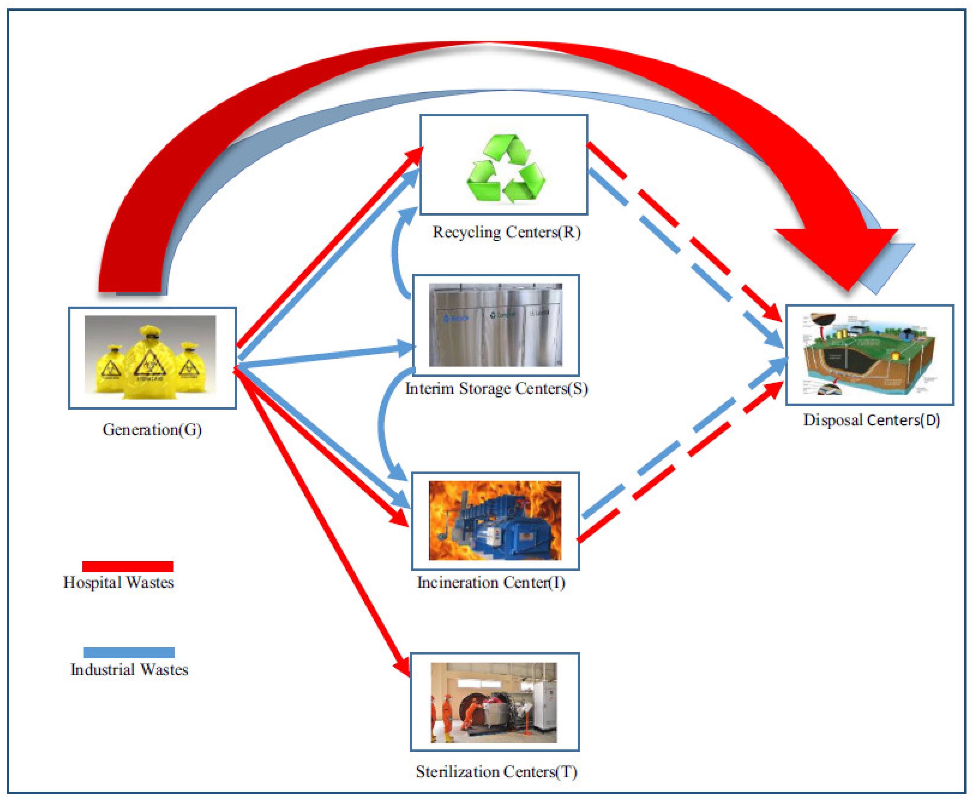
Figure 1 shows the sustainable hazardous material routing-locating problem. This figure shows the sustainable waste management system and hazardous material routing-locating problem. This picture links the economy and environmental aspects.

This issue is raised in rounds and questions such as the following: (1) How much product should be produced in each round? (2) Which customer’s demand should be answered in each round? (3) What is the optimal way to transfer materials to customers? Scientific studies are conducted to implement and apply in practical and real conditions [15]. Among the materials and goods with special conditions are dangerous materials and goods. The most important materials and goods are dangerous materials and goods [16].

This research has raised the problem of routing production for hazardous materials according to the conditions of these materials and considering the risk of distribution for the first time. The objective function of the problem that seeks to reduce the risk related to the distribution of hazardous materials has been modeled with a new approach corresponding to the production routing problem in a nonlinear way. The risk assessment in this research is related to the amount of car loading, the population at risk, and the type of hazardous substance. Also, by using a piecewise approximation, the model becomes a mixed integer, and the solution results are obtained and compared in two linear and nonlinear modes. The purpose is to arrive at an answer that considers the choices of the decision-makers in charge of hazardous material shipping and striking an equilibrium between different objectives of minimizing transportation risk and expense.

In Section 2, the literature of the investigated subject is stated. Section 3 describes the mathematical model of the problem, and the linearization of the mathematical model is presented in Section 4. Section 5 is dedicated to the sensitivity analysis related to the impact of hazardous materials on the production routing problem. Finally, in Section 6, conclusions and future suggestions are presented.

2. Research Background

The transportation problem is an important network-structured linear programming problem that arises in different fields of the distribution of materials and goods and has received much attention from researchers in the literature [17]. The transportation of hazardous materials may be classified among the general category of cargo transportation problems, and what differentiates the shipment of hazardous materials from the transportation of other materials is the risk associated with the accidental release of hazardous materials during transportation [18]. Hazardous materials can be transported by road, rail, sea, air, and pipeline. In each of these modes of transportation, the risk related to the transfer is evaluated and modeled by a special method. Road transportation is the most important mode for distributing hazardous materials [12]. The first approaches to optimize transporting hazardous materials are related to the 1970s. Kalelkar and Brooks [19] proposed a multidimensional framework for decision analysis to improve the support of transportation of hazardous materials. Risk assessment and planning of transportation of hazardous materials are two main research fields in the transportation of hazardous materials [18]. They proposed a multi-device framework under uncertainty [20].

In conducting research, many things have been completed to bring the problem closer to real conditions. For example, stating the problem of routing under the wireless sensor network in different cases brings the problem closer to real conditions [21]. Based on this issue, Erkut et al. [22] presented a simple classification for various aspects of the routing problem of hazardous materials, including risk assessment, routing, location, combined routing, and network design. They reviewed research based on types of transportation modes. Bianco et al. [23] proposed a new category called toll determination policies.

Vehicle routing is one of the issues that has received more attention in the distribution of dangerous substances. Bula et al. [24] discussed the distribution of hazardous materials in the problem of routing hazardous materials. In this research, the objective function is to reduce the risk related to the distribution of dangerous substances. The problem’s goal has been proposed nonlinearly and depends on the amount of car loading and the population at risk.

The same authors discussed the distribution of hazardous materials in the vehicle routing problem despite the contradictory goals of reducing risk and total cost in a dual-objective manner [3]. Du et al. [25] presented the distribution of hazardous materials in multi-depot vehicle routing problems. The authors explained the problem as two-level fuzzy planning.

Men et al. [26] proposed the distribution of hazardous materials to solve the problem of routing heavy vehicles to reduce risk. In this research, risk assessment using fuzzy variables is considered. Also, two meta-heuristic methods of a genetic algorithm and an adaptive large neighborhood search have been used to solve the model. Zhou et al. [27] proposed the distribution of hazardous materials in a multi-depot vehicle routing problem. In this issue, the model has been expressed as a dual-objective model to reduce risk and cost.

The design of the distribution network also involves the distribution of hazardous materials, more so than other issues of concern to researchers. In 2018, Fontin and Miner raised the problem of designing a distribution network of hazardous materials with the two opposite goals of risk reduction and total cost reduction. The problem is presented in a two-level form and solved by Bandar’s algorithm [28].

Zhang et al. [29] presented the design of the distribution network of hazardous materials using two-level planning based on the policies for determining complications. The problem model has been solved using the double refrigeration simulation algorithm. Fontaine et al. [30] suggested the design of the distribution network of hazardous materials in the form of two-level planning to reduce the government’s risk and the transport companies’ total cost. Risk assessment for this problem is based on the population.

Mohabbati-Kalejahi and Vinel [31] proposed the distribution of hazardous materials in the framework of the design of the closed-loop supply chain network (CLSCN) in such a way that allowed for the problem of determining the location of emergency rescue teams in the network at the same time. Ziaei and Jabbarzadeh proposed the distribution of hazardous materials in the routing-location problem with a multi-state distribution system and non-deterministic demand [32].

Tasouji Hassanpour and Tulett [33] also presented the distribution of hazardous materials in the problem context. Boalhosni et al. [34] described the distribution of hazardous materials in the problem of inventory positioning-routing by considering elastic demand and investigating queuing systems. The distribution of hazardous materials in a multi-objective inventory location-routing problem with the approach of the impact of distribution risk on environmental criteria was proposed by Rahbari et al. [35].

Fang [36] reviewed the application of environmental criteria in the routing problem. Salamatbakhsh et al. [37] considered minimizing the cost of vehicles and maximizing the satisfaction of vehicle drivers through optimizing service time in the case of uncertainty of transit times. Another basic issue is the problem of production routing, which has already been the focus of researchers. This issue deals with simultaneous decision-making about the amount of production, the amount of inventory in warehouses, and the amount and route of distribution of materials. Most of the existing studies in the field of production routing problems consider the level of tactical decisions [38]. Low et al. [39] presented the problem of routing production in a two-level SC by a heterogeneous transport fleet. Li et al. [40] proposed the reverse chain of returning defective goods from customers to suppliers in the issues of vehicle routing and inventory routing under the title of sending and receiving. This issue was raised for the first time in 2020 by Hemmati Golsefidi and Akbari Jokar on the issue of production routing [41].

Emamian et al. [42] proposed the release of environmental pollutants by the factory in addition to the release related to distribution in the production routing problem. Also, considering customers’ returns of defective goods, they considered social criteria. For the first time, Schenekemberg et al. [43] raised the issue of routing production in two levels of supply and demand for chemicals.

In addition to the above, additional information has also been considered in the research of models related to production routing. The service time for loading and unloading goods and the shipping time have been considered by [44,45]. The research has regarded the loading and unloading times in two ways. One determines the maximum time to complete routes [46], and the other determines customer time windows [45]. Sending a batch of products has been proposed by the research of Ganji et al. [47].

Li et al. [40] suggested that the lifespan of the products is affected by the time they are sent, and they should reach the consumer in the shortest possible time because the price is determined based on the remaining life of the products.

The impacts and difficulties of the COVID-19 pandemic on global waste management for sustainable development were evaluated by Abbasi and Sıcakyüz [48]. Sarbijan and Behnamian studied the real-time collaborative feeder vehicle routing problem with flexible time frames [49]. A distribution network for necessities in the event of COVID-19 and earthquakes simultaneously was constructed [50]. The COVID-19 pandemic was considered when designing the location-routing problem for a cold supply chain [51]. Abbasi et al. [52] simulated a COVID-19-era financial and logistical supply chain network (SCN). A study was conducted on the hybrid meta-heuristic approach for the multi-fleet feeder vehicle routing problem by Sarbijan and Behnamian [53,54]. A two-finger haptic robotic hand with unique stiffness sensing and impedance control was created by Mohammadi et al. [55]. A meta-heuristic method and a mathematical model addressed the real-time feeder truck routing issue.

Table 1. Comparative evaluation of the key findings from earlier studies.

Articles	Production Routing	Network Design	Routing	Inventory Routing	Environment	Social	Economic	Risk	Cost	Single Period	Multi-Period	Linear	Nonlinear
Bula et al. (2016) [6]			*			*		*		*			*
Du et al. (2017) [25]			*				*	*		*		*
Fontain and Miner (2018) [28]		*				*		*	*	*		*
Bula et al. (2019) [3]			*				*		*	*			*
Men et al. (2019) [26]			*		*			*			*	*
Zhang et al. (2019) [29]		*			*			*		*		*
Fontain et al. (2020) [30]		*					*		*	*		*
Mohabbati-Kalejahi & Vinel (2021) [31]		*					*	*	*	*		*
Zhou et al. (2021) [27]			*				*	*	*	*		*
Ziaei and Jabarzadeh (2021) [32]			*		*		*		*	*		*
Bolhasani et al. (2021) [34]				*		*	*		*		*	*
Tasouji Hassanpour (2022) [33]			*				*		*	*		*
Rahbari et al. (2022) [35]				*	*		*	*			*		*
This research	*				*	*		*			*		*

* means having the concept of issue.

shows the main indicators of past research and future research on the problem of the distribution of dangerous substances in a comparative manner.

Despite the work completed by researchers in production routing, the research process in hazardous materials distribution shows that few studies have comprehensively addressed the mutual effects of these two problems. Meanwhile, the mutual effects of these two issues on each other can help management decisions to improve the general situation of production and distribution of dangerous substances. Among the existing studies in the field of minimizing the risk of the transportation of hazardous materials, no attention has been paid to the impact of the production schedule of these materials, i.e., the production volume and production time. Most studies have paid attention to the effects of routing on risk. Attention to accidents related to the transportation of dangerous substances is more due to the wide range of unfortunate consequences. The extent and catastrophic nature of the events are reflected in some of the past risk assessment models.

Sustainability criteria, especially economic criteria, have always been considered by researchers, but the research trend shows that researchers are increasingly paying attention to two social and environmental criteria. Hazardous materials are among the materials that threaten the health of society and the environment. Production routing issues are usually raised with economic goals. However, when raised in dangerous substances, the same problem is raised with a more important goal besides the economic goals: reducing the risk of producing and distributing hazardous substances. This makes the issue attractive for researchers and decision-making managers.

In this article, for the first time, the optimal production volume and time have been considered in addition to routing in a routing model to produce hazardous materials and to minimize the risk. To reflect this idea, a suitable nonlinear risk function has been used depending on the amount of car loading, the population at risk, and the type of hazardous substance. In this model, variables related to the amount of production and loading of vehicles and limitations for the linearization of the nonlinear model have been considered, which have not been seen in the previous production routing models. In the following, the research problem and its results will be discussed.

Sustainability criteria, especially economic criteria, have always been considered by researchers, but the research trend shows scholars are increasingly paying attention to two social and environmental criteria. Hazardous materials are among the materials that threaten the health of society and the environment. Production routing issues are usually raised with economic goals. However, when raised in the field of dangerous substances, the same problem is raised with a more important goal than the economic goals: reducing the risk of the production and distribution of dangerous substances. This makes the issue attractive for researchers and decision-making managers.

In this paper, for the first time, the optimal production volume and time have been considered in addition to routing in a routing model to produce hazardous materials and to minimize the risk. To reflect this idea, a suitable nonlinear risk function has been used depending on the amount of car loading, the population at risk, and the type of hazardous substance. In this model, variables related to the amount of production and loading of vehicles and limitations for the linearization of the nonlinear model have been considered, which have not been seen in the previous production routing models. In the following, the research problem and its results will be discussed.

3. Statement of the Problem

Considering the dangerous nature of the materials in question and the importance of their social and environmental effects, the most important issue is the correct risk assessment and modeling so they can reflect the reality in the area well. Therefore, the objective function of the proposed production routing problem is to minimize the total cost in this research. The risk function considered in the problem model to evaluate the reality related to the problem’s criteria depends on the machine’s loading, the population at risk, and the type of hazardous substance. Considering this issue, the objective function of the problem is a nonlinear function that considers risk minimization. The problem is raised as a single target in a one-level SC.

In this research, the problem is raised in a one-level SC. Decision-making in the SC is completed centrally and by a decision-maker who is a producer. The problem is raised in rounds, and at the beginning of each period, the amount of inventory of the customers’ and producers’ warehouses is known, and the demand for each customer in each period is certain and limited. The factory’s production amount, the inventory in the warehouses of customers and the factory, the amount of transfer of materials to each customer, and the route of transfer of materials to customers in each period are among the decision variables related to the problem. The transport fleet is associated with the distribution of homogeneous materials and has a limited and certain capacity. The use of any of the distribution machines has a transfer risk. The mathematical model of the problem is proposed as a single product, multi-round, single factory, and single target. The sets and indices related to the mathematical model of the problem are presented in

Table 2. Sets.

Index	Definition
$i$	The node of the customers $i=\{1,‥,I\}$
$j$	The node of the factories $j=\{1,‥,J\}$
$k$	The available vehicles $k=\{1,‥,K\}$
$t$	The periods $t=\{1,‥,T\}$

.

The assumptions that will be considered in the stages of the modeling analysis and evaluation include the following:

• Customers’ demands must be fully met in every period.
• Distances of points are considered Euclidean.
• The position of producers and customers is fixed and certain.
• Customer demand is known and fixed, and each customer should be visited only once by one vehicle in each period.
• The transportation fleet is homogeneous, and each car can be started once during each period.
• The capacity of vehicles and the inventory capacity of producers’ and customers’ warehouses are limited and specific.
• The paths created should only start from the manufacturer and end with the manufacturer.
• Customer demand is the same and constant in all periods.
• The production capacity of the factory is fixed and limited in each period.

3.1. Mathematical Model of the Problem

The sets and parameters in the mathematical model of the problem and their definitions are presented in Table 2 and

Table 3. Parameters.

Parameter	Definition
$de{m}_i^t$	The demand of customer i in period t
$di{s}_{ij}$	The distance between two nodes, i and j
${\phi }_{ij}$	The number of populations at risk of dangerous substance release between two nodes, i and j
${\theta }_k$	The accident rate of vehicle k per kilometer
$\mathrm{Pr}$	The possibility of release of dangerous substances in accidents
$Ca{p}_k$	The capacity of vehicle k
$A\&B$	Values depending on the type of hazardous materials
$U_i$	Maximum capacity of node i
$L_i$	Minimum capacity of node i
${\pi }_j^t$	The capacity of production the factory j in period t

.

Table 4. Variables.

Variable	Definition
$y_{ij}^{kt}$	If the route from node i to node j is used by vehicle k in period t, it equals 1; otherwise, it equals 0
$Q_j^t$	The amount of production in factory j in period t
$Q{S}_{ik}^t$	The amount of shipment to customer i in period t by vehicle k
$Q{L}_{ij}^{kt}$	The amount of loading of vehicle k on the route from node i to node j in period t
$I_i^t$	The amount of inventory in the warehouse of customer i in period t
$I_j^t$	The amount of inventory in the warehouse of factory j in period t

shows the variables of the model and the meaning of each of them. The objective function (Z) is the risk reduction objective function.

$$MinZ=\mathrm{Pr}\times B\times {\displaystyle \sum _{k\in K}{\displaystyle \sum _{t\in T}{\displaystyle \sum _{i\in I}{\displaystyle \sum _{j\in J}{(Q{L}_{ij}^{kt})}^A\times {\theta }_k\times {\mathit{dis}}_{ij}\times {\phi }_{ij}}}}}$$

(1)

$$I_j^t=I_j^{t-1}+Q_j^t-{\displaystyle \sum _{i\in I}{\displaystyle \sum _{k\in K}Q{S}_{ik}^t}}\hspace{1em}\hspace{1em}\forall t\in T$$

(2)

$$I_i^t\le U_i\hspace{1em}\forall i\in I,t\in T$$

(3)

$$I_i^t\le L_i\hspace{1em}\forall i\in I,t\in T$$

(4)

$$I_i^t=I_i^{t-1}+{\displaystyle \sum _{k\in K}Q{S}_{ik}^t}-de{m}_i^t\hspace{1em}\forall t\in T,i\in I$$

(5)

$$Q_j^t\le {\pi }_j^t\hspace{1em}\forall t\in T \forall j\in J$$

(6)

$$Q_j^t\le U_i- I_i^{t-1}\hspace{1em}\forall t\in T$$

(7)

$${\displaystyle \sum _{k\in K}Q{S}_{ik}^t}\le U_i-I_i^{t-1}\hspace{1em}\forall t\in T,i\in I$$

(8)

$$Q{S}_{ik}^t\le U_i\times {\displaystyle \sum _{j\in J}{y}_{ij}^{kt}}\hspace{1em}\forall t\in T,i\in I,k\in K$$

(9)

$$Q{S}_{ik}^t\le Ca{p}_k\times {\displaystyle \sum _{j\in J}{y}_{ij}^{kt}}\hspace{1em}\forall t\in T,i\in I,k\in K$$

(10)

$${\displaystyle \sum _{i\in I}{\displaystyle \sum _{k\in K}{y}_{ij}^{kt}\le 1}}\hspace{1em}\forall t\in T,j\in J$$

(11)

$${\displaystyle \sum _{i\in I}{y}_{ij}^{kt}}+{\displaystyle \sum _{i\in I}{y}_{ij}^{kt}}=2\times {\displaystyle \sum _{i\in I}{y}_{ij}^{kt}}\hspace{1em}\forall t\in T,j\in J,k\in K$$

(12)

$$y_{ij}^{kt}=0\hspace{1em}\forall t\in T,i\in I,k\in K$$

(13)

$${\displaystyle \sum _{i\in I}Q{L}_{ik}^t}={\displaystyle \sum _{i\in I}Q{S}_{ik}^t}\hspace{1em}\forall t\in T,k\in K$$

(14)

$$Q{L}_i^{kt}=0\hspace{1em}\forall t\in T,i\in I,k\in K$$

(15)

$$Q{L}_{ij}^{kt}\le Ca{p}_k\times y_{ij}^{kt}\hspace{1em}\forall t\in T,\forall i\in I,\forall j\in J,k\in K$$

(16)

$$y_{ij}^{kt}\in \{0,1\}\hspace{1em}\forall t\in T,\forall i\in I,\forall j\in J,k\in K$$

(17)

$$Q_j^t,Q{S}_{ik}^t,Q{L}_{ij}^{kt},I_i^t\ge 0\hspace{1em}\forall t\in T,\forall i\in I,\forall j\in J,k\in K$$

(18)

The objective function in Equation (1) shows that it minimizes the risk caused by the distribution of dangerous substances and their consequences. In this regard, four factors of accident probability, the probability of release of hazardous substances, the rate of release of dangerous substances, and the population at risk per unit of distance have been used to express risk. The two constants A and B also consider the effects related to the type of hazardous substance. Equation (2) states that the inventory of the factory in each period is equal to the inventory of the previous period plus the amount of production in that period minus the amount of goods to customers. Equations (3) and (4) determine warehouses’ maximum and minimum capacity limits, respectively. Equation (5) states that the inventory level of customers’ warehouses in each period is equal to the amount of inventory of the previous period plus the number of goods received in that period, minus the demand of the desired customer. Equations (6) and (7) control the amount of factory production in each period. Equation (8) considers the shipment amount for each customer in proportion to the amount of demand and its stock in each period. Equations (9) and (10) control the amount of cargo sent to customers in each period according to the capacity of warehouses and machines so that it does not exceed the allowed limit.

Equation (11) guarantees that each customer should be visited by only one machine in each period. Also, Equations (12) and (13) prevent creating a sub-network. Equations (14) and (15) show that the amount of car loading at the beginning of the route should equal the amount of load allocated to that route’s customers and zero at the end of the route. Equation (16) applies the machine capacity limit to the amount of machine loading. Finally, Equations (17) and (18) show the type and sign of the model variables.

3.2. Linearization

Considering that the risk reduction objective function introduced in the model is nonlinear and dealing with nonlinear objective functions increases the solution time and reduces the quality of the answer in a reasonable time, in this research, the piecewise approximation method for the objective function has been used to solve the model. In the following, the linear approximated objective function is presented along with the relevant constraints. Then the model is solved in both nonlinear and linear ways, and the results are compared [6].

The variable ${(Q{L}_{ij}^{kt})}^A$ in the objective function is presented in a nonlinear way. This variable is further expressed using piecewise approximation in the objective function. The limited interval $[Q_0,Q_N]$ for the nonlinear variable ${(Q{L}_{ij}^{kt})}^A$ is divided into $N$ pieces $\{l_0,\dots ,l_N\}$ incrementally and sequentially. The value ${(Q{L}_{ij}^{kt})}^A$ is approximated by a line that passes through the two starting and ending points in each section. Therefore, the variable value ${(Q{L}_{ij}^{kt})}^A$ is defined according to the Equation (19).

$${(Q{L}_{ij}^{kt})}^A=\left\{x_n+y_{n}Q{L}_{ij}^{kt},Q{L}_{ij}^{kt}\in \left[l_{n-1},l_n\right]\forall n\in \left\{1,\dots ,N\right\}\right\}$$

(19)

In the above relationship, $x_n\in R$ and $y_n\in R$ represent the width from the origin and the slope of the approximate line, respectively, and the relationship $l_0\prec l_1\prec \dots \prec l_N$ is also established. The variable $t_{ij}^{kt}$ is considered as an approximate linear value of the variable ${(Q{L}_{ij}^{kt})}^A$ and the value $t_0={(l_0)}^A$. Then, the approximated risk objective function is converted into a mixed integer model by defining the zero, one, and positive variables ${\omega }_{ij}^{kn},n=1,\dots ,N$. The variable $h_{ij}^{kn}$ calculates the difference, and ${\omega }_{ij}^{kn}$ calculates the distance variable between $Q{L}_{ij}^{kt}$ and $l_{n-1}$. The above approximation is stated in the following research [56]. The linear objective function and the constraints related to the approximated linear model for each variable are Equations (20)–(26).

$$t_{ij}^{kt}=t_0+{\displaystyle \sum _{n=1}^N{x}_n}\times {\omega }_{ijk}^{nt}\hspace{1em}\forall i\in I,j\in J,i\ne j,k\in K,t\in T$$

(20)

$$Q{L}_{ij}^{kt}=l_0+{\displaystyle \sum _{n=1}^N{\omega }_{ijk}^{nt}}\hspace{1em}\forall i\in I,j\in J,i\ne j,k\in K,t\in T$$

(21)

$${\omega }_{ijk}^{1t}\le l_1-l_0\hspace{1em}\forall i\in I,j\in J,i\ne j,k\in K,t\in T$$

(22)

$${\omega }_{ijk}^{nt}\ge (l_n-l_{n-1})h_{ijk}^{nt}\hspace{1em}\forall i\in I,j\in J,i\ne j,k\in K,t\in T,n=1,\dots ,N-1$$

(23)

$${\omega }_{ijk}^{n+1t}\le (l_{n+1}-l_n)h_{ijk}^{nt}\hspace{1em}\forall i\in I,j\in J,i\ne j,k\in K,t\in T,n=1,\dots ,N-1$$

(24)

$$h_{ijk}^{nt}\in \{0,1\}\hspace{1em}\forall i\in I,j\in J,i\ne j,k\in K,t\in T,n=1,\dots ,N-1$$

(25)

$${\omega }_{ijk}^{nt},t_{ij}^{kt}\ge 0\hspace{1em}\forall i\in I,j\in J,i\ne j,k\in K,t\in T,n=1,\dots ,N-1$$

(26)

4. Numerical Results

In this section, we evaluate the quality of the linear approximation and check the results of solving the production routing model. To determine the parameters related to solving the problem, a fixed interval from the uniform function methodLINGO19 is used on a notebook equipped with an Intel Core i7 2.40 GHz CPU and 8 GB RAM to solve the remaining parameters found in all four models. Computational times vary from 3 to 19 s; running complex numerical examples is acceptable. The model’s parameters can be found in

Table 5. Suggested model parameter values.

Parameters	Values	Parameters	Values
$de{m}_i^t$	Uniform (1,900)	$Ca{p}_k$	Uniform (1,2000)
$di{s}_{ij}$	Uniform (1,10,000)	$A\&B$	Uniform (1,100)
${\phi }_{ij}$	Uniform (1,500)	$U_i$	Uniform (1,1000)
${\theta }_k$	Uniform (1,500)	$L_i$	Uniform (1,500)
$\mathrm{Pr}$	Uniform (0,1)	${\pi }_j^t$	Uniform (1,1000)

. The ideal value solution for objective functions is displayed in Table 5.

As it is clear from the obtained results, the piecewise approximation of the problem’s nonlinear objective function has produced better results than the nonlinear model in all samples. The significant difference between the two values of the nonlinear objective function with the same solution time indicates the effectiveness of the desired linear approximation. This is despite that, in general, collaborating with linear models is easier and more diverse than with nonlinear models. The diagram in Figure 2 clearly shows the obtained results.

5. Sensitivity Analysis

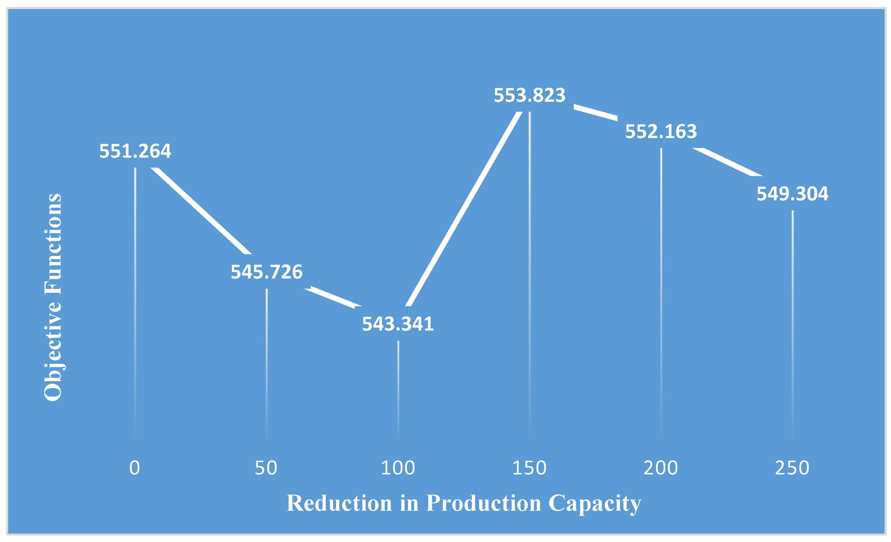
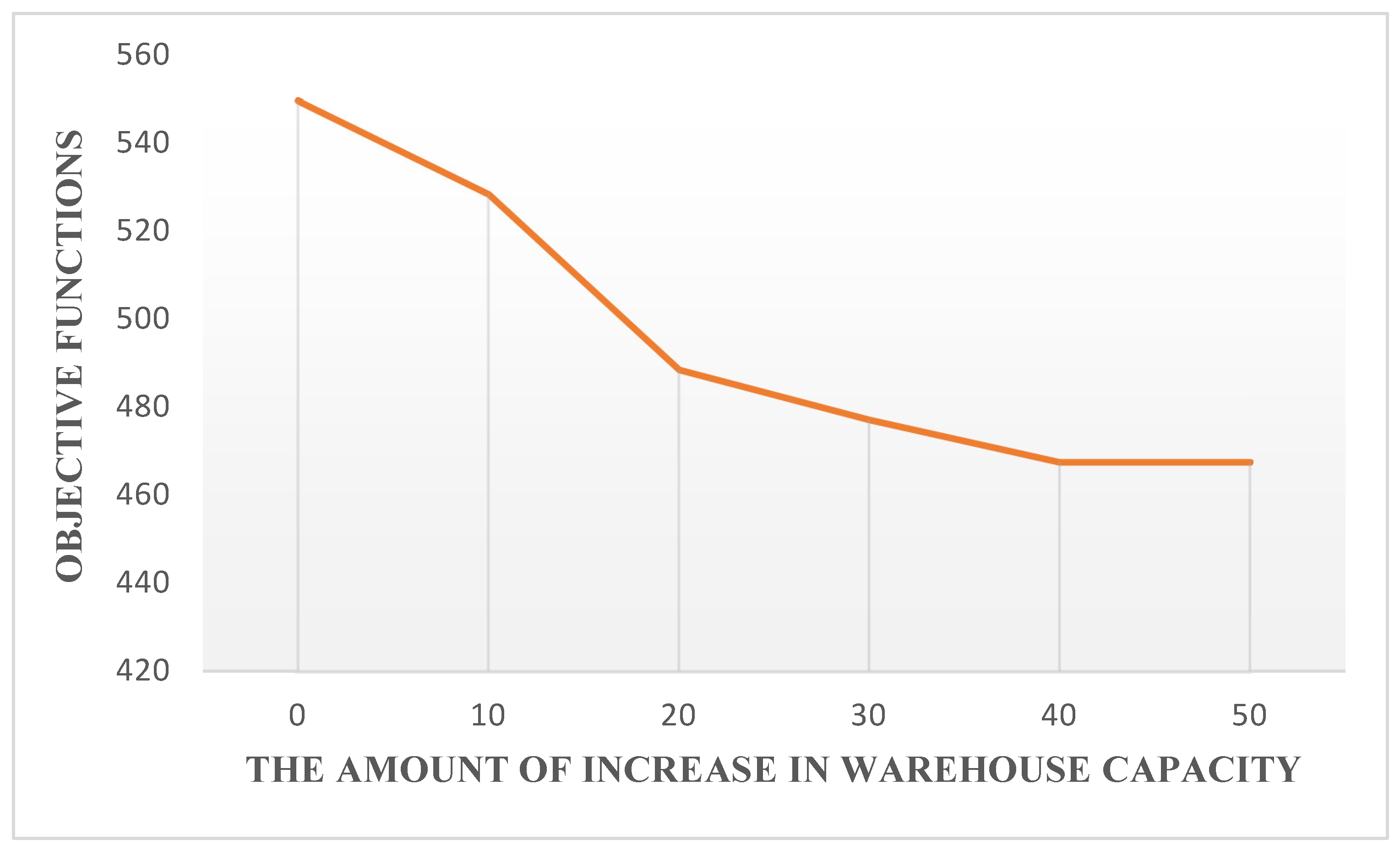
The purpose of the model is to reduce the risk caused by the distribution of dangerous substances and among the cases that can be better managed by making the right decision about the risk caused by the distribution of hazardous substances at the level of the SC, the inventory capacity of the warehouses, and the production capacity of the factory in each period. In this section, two parameters of the maximum capacity of the warehouses and the production capacity are presented to investigate the effects related to the parameters of the sensitivity analysis model. Due to the better answers related to the linear approximation model, a linear model was used to compare and obtain results in the sensitivity analysis. What is dangerous is the transfer of hazardous materials from the factory to the customer’s warehouse. Of course, the amount of machine loading is also an influencing factor in the risk of distribution, which has a smaller effect than the number of transfers. Suppose it is possible to use the largest volume of transfer by machine by changing the capacity of warehouses and production capacity. In that case, we can witness the reduction in the number of transfers and, subsequently, the reduction in the risks caused by it. To investigate this issue in detail in this research, a sensitivity analysis was conducted by changing the maximum capacity of warehouses and the production capacity of factories and re-examining and solving the model. First, the capacity of the warehouses was examined step by step, with increments of 10 units at each stage. These increases have continued to the point where they no longer affect the solution to the problem. In the next step, by reducing the production capacity by 50 units stepwise until the problem is solvable, the model has been solved, and the related results can be seen in

Table 6. The results of solving the model in two linear and nonlinear modes.

Problems	Nonlinear Model	Linear Approximation Model
P1	605.059	502.139
P2	576.251	550.189
P3	1082.584	963.954
P4	1195.829	988.726
P5	1197.134	1074.169
P6	1205.456	1064.941
P7	2222.365	2031.223
P8	2462.785	2233.829

.

It should be noted that the rest of the parameters in the model have not changed. The model has also been checked in all cases; for example, ABS1_15_1 had 14 customers and was solved with the same processing system. In addition, the amount of the nonlinear objective function corresponding to the variables obtained by the linear model has been compared.

Table 7. The effect of changing model parameters on the objective function.

Percentage of Changes	The Value of Objective Function with Changes in Warehouse Capacity	Percentage of Changes	The Value of Objective Function with Changes in Production Capacity
0	549.642	0	551.264
+10	528.479	−50	545.726
+20	488.542	−100	543.341
+30	477.217	−150	553.823
+40	467.542	−200	552.163
+50	467.542	−250	549.304

shows the effect of changing model parameters on the objective function.

The results related to the change in production capacity are shown in Figure 3 as a linear diagram. As is clear from the graph and table of results, reducing production capacity to 1000 units had a small effect on reducing the risk. This problem is because the reduction in production has caused the model only to try to meet customer demand and less to fill the warehouses, and this has caused the same number of trucks to be carried out but with a lower loading rate. Less machine loading will subsequently reduce the risk. However, with a decrease of about 1500 units in the model’s production capacity, it is forced to supply all the demand in its respective periods, and this causes the number of transfers in each period to increase. Subsequently, the related risk also increases. In general, what is noticeable is that the change in the production capacity does not impact the risk of the distribution of dangerous substances. Considering the indirect effect of the production capacity on the number of transfers, this issue seems logical. Despite the small impact of the production capacity, considering the high importance of the risks caused by the distribution of dangerous substances, this small effect should not be ignored in managing the production and distribution of hazardous substances.

Figure 4 shows the diagram related to the impact of warehouse capacity changes on the risk of the distribution of dangerous substances. As it is clear from the numbers in the table, the effect of the warehouse capacity is more than that of the production capacity on the distribution risk. For example, an increase of 20 points in the capacity of factory and customer warehouses has reduced the risk by 63 points. Increasing the capacity of warehouses makes it possible to use the maximum capacity of machines for distribution in every transfer. This problem reduces the number of transportations in different periods, reducing the risk of the distribution of dangerous substances.

It should be noted that these changes can affect the amount of risk to some extent. The graph shows that the increase in changes after about 30 units with a slight slope affects the risk, and to some extent, it becomes ineffective. This problem is caused by the fact that even if the warehouse capacity increases, the machines distribute at full capacity, and the machines do not have more processing power and do not have much of an effect on the number of trips and related risks. Considering the importance and risks of the distribution of dangerous substances, management decisions can reduce the risks as much as possible by changing the problem’s parameters. However, this issue should be addressed to establish the best balance between other factors, such as the cost and potential limitations.

6. Conclusions and Recommendations for Future Research

This research has investigated the issue of production routing for hazardous materials to reduce risk. The risk objective function related to the mathematical model has been presented in a nonlinear way, and it has been converted into a linear integer function with a piecewise approximation. The relevant results have been investigated in both cases, and the results have been compared. The obtained results clearly show the quality of the approximation used to solve the problem as well as one of the other defects related to solving the nonlinearity of the model. To check the quality of the answers at different times, the authors tried to limit the time of solving the problem to other numbers. Interestingly, the nonlinear model could not reach a feasible solution in the above times. Meanwhile, the linear approximation model provides a viable solution in less than 70 s.

The sensitivity analysis clearly shows the effects of the warehouse and factory production capacity on the number of transfers related to the distribution of hazardous materials and the direct impact on the relevant risk. This issue can be a lever for managers and decision-makers to use to better control the risk of transportation operations, according to the desired facilities and budget. Also, in a supply chain where decisions are made centralized, the correct management of the influencing parameters in the model can significantly reduce the risk and damages related to the distribution of dangerous substances.

There are also limitations in the model, such as the optimization of costs related to the model not being considered. However, costs can be controlled by determining the upper and lower limits of the inventory. Another limitation is the time to solve problems. Although the linearization of the mathematical model reduces the time to solve the problem, it still takes a long time to solve large problems. Also, the problem model is expressed as a single product, while many manufacturers produce several products simultaneously.

As a suggestion for future research, the expression of the model in a dual-objective form, which seeks to reduce the risk and total cost simultaneously, can be considered. It is also interesting to present effective meta-heuristic algorithms that can provide a suitable solution for a large-scale problem in a reasonable time. Also, the development of the multi-product model can bring the problem closer to the real situation.

References

1. Romero, N.; Nozick, L.K.; Xu, N. Hazmat facility location and routing analysis with explicit consideration of equity using the Gini coefficient. Transp. Res. Part E Logist. Transp. Rev. 2016, 89, 165–181. [Google Scholar] [CrossRef]
2. Pajić, V.; Andrejić, M.; Jolović, M.; Kilibarda, M. Strategic warehouse location selection in business logistics: A novel approach using imf SWARA–MARCOS—A case study of a Serbian logistics service provider. Mathematics 2024, 12, 776. [Google Scholar] [CrossRef]
3. Bula, G.A.; Afsar, H.M.; González, F.A.; Prodhon, C.; Velasco, N. Bi-objective vehicle routing problem for hazardous materials transportation. J. Clean. Prod. 2019, 206, 976–986. [Google Scholar] [CrossRef]
4. Safaeian, M.; Moses, R.; Ozguven, E.E.; Dulebenets, M.A. An optimization-based risk management framework with risk interdependence for effective disaster risk reduction. Prog. Disaster Sci. 2024, 21, 100313. [Google Scholar] [CrossRef]
5. An, F.P.; Liu, J.E.; Bai, L. Object recognition algorithm based on optimized nonlinear activation function-global convolutional neural network. Vis. Comput. 2022, 38, 541–553. [Google Scholar] [CrossRef]
6. Bula, G.A.; Gonzalez, F.A.; Prodhon, C.; Afsar, H.M.; Velasco, N.M. Mixed integer linear programming model for vehicle routing problem for hazardous materials transportation. IFAC-Pap. 2016, 49, 538–543. [Google Scholar] [CrossRef]
7. Camponogara, E.; Seman, L.O.; Müller, E.R.; Miyatake, L.K.; Gaspari, E.F.; Vieira, B.F.; Pacheco, B.M. A ReLU-based Linearization Approach for Maximizing Oil Production in Subsea Platforms: An Application to Flow Splitting. Chem. Eng. Sci. 2024, 295, 120165. [Google Scholar] [CrossRef]
8. Díaz-Madroñero, M.; Mula, J.; Jiménez, M.; Peidro, D. A rolling horizon approach for material requirement planning under fuzzy lead times. Int. J. Prod. Res. 2017, 55, 2197–2211. [Google Scholar] [CrossRef]
9. Armentano, V.A.; Shiguemoto, A.L.; Løkketangen, A. Tabu search with path relinking for an integrated production–distribution problem. Comput. Oper. Res. 2011, 38, 1199–1209. [Google Scholar] [CrossRef]
10. Adulyasak, Y.; Cordeau, J.-F.; Jans, R. The production routing problem: A review of formulations and solution algorithms. Comput. Oper. Res. 2015, 55, 141–152. [Google Scholar] [CrossRef]
11. Chandra, P.; Fisher, M.L. Coordination of production and distribution planning. Eur. J. Oper. Res. 1994, 72, 503–517. [Google Scholar] [CrossRef]
12. Holeczek, N. Hazardous materials truck transportation problems: A classification and state of the art literature review. Transp. Res. Part D Transp. Environ. 2019, 69, 305–328. [Google Scholar] [CrossRef]
13. Aydemir-Karadag, A. A profit-oriented mathematical model for hazardous waste locating-routing problem. J. Clean. Prod. 2018, 202, 213–225. [Google Scholar] [CrossRef]
14. Raeisi, D.; Jafarzadeh Ghoushchi, S. A robust fuzzy multi-objective location-routing problem for hazardous waste under uncertain conditions. Appl. Intell. 2022, 52, 13435–13455. [Google Scholar] [CrossRef]
15. Fortes, A.; Camargo, R.; Muniz, L.R.; de Souza Lima, F.M.; dos Reis Cota, F. Efficient metaheuristics to solve a rich production-routing problem. Comput. Ind. Eng. 2022, 171, 108369. [Google Scholar] [CrossRef]
16. Erkut, E.; Verter, V. Modelling of transport risk for hazardous materials. Oper. Res. 1998, 46, 625–642. [Google Scholar] [CrossRef]
17. Kane, L.; Diakite, M.; Kane, S.; Bado, H.; Konate, M.; Traore, K. A new algorithm for fuzzy transportation problems with trapezoidal fuzzy numbers under fuzzy circumstances. J. Fuzzy Ext. Appl. 2021, 2, 204–225. [Google Scholar] [CrossRef]
18. Bianco, L.; Caramia, M.; Giordani, S. A bilevel flow model for hazmat transportation network design. Transp. Res. Part C Emerg. Technol. 2009, 17, 175–196. [Google Scholar] [CrossRef]
19. Kalelkar, A.S.; Brooks, R.E. Use of multidimensional utility functions in hazardous shipment decisions. Accid. Anal. Prev. 1978, 10, 251–265. [Google Scholar] [CrossRef]
20. Pourghader Chobar, A.; Sabk Ara, M.; Moradi Pirbalouti, S.; Khadem, M.; Bahrami, S. A multi-objective location-routing problem model for multi-device relief logistics under uncertainty using meta-heuristic algorithm. J. Appl. Res. Ind. Eng. 2022, 9, 354–373. [Google Scholar] [CrossRef]
21. Fan, L. A Short Study of the Components and Applications of Wireless Sensor Network. Big Data Comput. Vis. 2022, 2, 101–106. [Google Scholar] [CrossRef]
22. Erkut, E.; Tjandra, S.A.; Verter, V. Handbooks in Operations Research and Management Science, 1st ed.; Elsevier: Amsterdam, The Netherlands, 2007. [Google Scholar]
23. Bianco, L.; Caramia, M.; Giordani, S.; Piccialli, V. International Series in Operations Research and Management Science; Springer: Berlin/Heidelberg, Germany, 2013. [Google Scholar]
24. Bula, G.A.; Prodhon, C.; Gonzalez, F.A.; Afsar, H.M.; Velasco, N. Variable neighborhood search to solve the vehicle routing problem for hazardous materials transportation. J. Hazard. Mater. 2017, 324, 472–480. [Google Scholar] [CrossRef]
25. Du, J.; Li, X.; Yu, L.; Dan, R.; Zhou, J. Multi-depot vehicle routing problem for hazardous materials transportation: A fuzzy bi-level programming. Inf. Sci. 2017, 399, 201–218. [Google Scholar] [CrossRef]
26. Men, J.; Jiang, P.; Xu, H. A chance constrained programming approach for HazMat capacitated vehicle routing problem in Type-2 fuzzy environment. J. Clean. Prod. 2019, 237, 117754. [Google Scholar] [CrossRef]
27. Zhou, Z.; Ha, M.; Hu, H.; Ma, H. Half open multi-depot heterogeneous vehicle routing problem for hazardous materials transportation. Sustainability 2021, 13, 1262. [Google Scholar] [CrossRef]
28. Fontaine, P.; Minner, S. Benders decomposition for the Hazmat Transport Network Design Problem. Eur. J. Oper. Res. 2018, 267, 996–1002. [Google Scholar] [CrossRef]
29. Zhang, L.; Feng, X.; Chen, D.; Zhu, N.; Liu, Y. Designing a hazardous materials transportation network by a bi-level programming based on toll policies. Phys. A Stat. Mech. Its Appl. 2019, 534, 122324. [Google Scholar] [CrossRef]
30. Fontaine, P.; Crainic, T.G.; Gendreau, M.; Minner, S. Population-based risk equilibration for the multimode hazmat transport network design problem. Eur. J. Oper. Res. 2020, 284, 188–200. [Google Scholar] [CrossRef]
31. Mohabbati-Kalejahi, N.; Vinel, A. Robust hazardous materials closed-loop supply chain network design with emergency response teams’ location. Transp. Res. Rec. 2021, 2675, 306–329. [Google Scholar] [CrossRef]
32. Ziaei, Z.; Jabbarzadeh, A. A multi-objective robust optimization approach for green location-routing planning of multi-modal transportation systems under uncertainty. J. Clean. Prod. 2021, 291, 125293. [Google Scholar] [CrossRef]
33. Tasouji Hassanpour, S.; Ke, G.Y.; Tulett, D.M. A time-dependent location-routing problem of hazardous material transportation with edge unavailability and time window. J. Clean. Prod. 2021, 322, 128951. [Google Scholar] [CrossRef]
34. Bolhasani, P.; Fallah, M.; Tavakkoli-Moghaddam, R.; Alam-Tabriz, A. Presenting a multi-objective mathematical model of a location-routing-inventory problem for hazardous materials considering the concept elastic demand and queuing system. Decis. Oper. Res. (In Persian). 2022, 6, 210–241. [Google Scholar] [CrossRef]
35. Rahbari, M.; Arshadi Khamseh, A.; Sadati-Keneti, Y.; Jafari, M.J. A risk-based green location- inventory-routing problem for hazardous materials: NSGA II, MOSA, and multi-objective black widow optimization. Environ. Dev. Sustain. 2022, 24, 2804–2840. [Google Scholar] [CrossRef]
36. Fang, J. Smart phone based monitoring of agricultural activities. Comput. Algorithms Numer. Dimens. 2022, 1, 159–163. [Google Scholar] [CrossRef]
37. Salamatbakhsh, A.; Tavakkoli-Moghaddam, R.; Pahlevani, A. Solving a vehicle routing problem underuncertainty by a differential evolution algorithm. Inov. Manag. Oper. Strateg. (In Persian). 2021, 1, 310–319. [Google Scholar] [CrossRef]
38. Chen, Z.L. Integrated production and outbound distribution scheduling: Review and extensions. Oper. Res. 2010, 58, 130–148. [Google Scholar] [CrossRef]
39. Low, C.; Chang, C.M.; Li, R.K.; Huang, C.L. Coordination of production scheduling and delivery problems with heterogeneous fleet. Int. J. Prod. Econ. 2014, 153, 139–148. [Google Scholar] [CrossRef]
40. Li, Y.; Chu, F.; Chu, C.; Zhu, Z. An efficient three-level heuristic for the large-scaled multi-product production routing problem with outsourcing. Eur. J. Oper. Res. 2019, 272, 914–927. [Google Scholar] [CrossRef]
41. Hemmati Golsefidi, A.; Akbari Jokar, M.R. A robust optimization approach for the production- inventory-routing problem with simultaneous pickup and delivery. Comput. Ind. Eng. 2020, 143, 106388. [Google Scholar] [CrossRef]
42. Emamian, Y.; Kamalabadi, I.N.; Eydi, A. Developing and solving an integrated model for production routing in sustainable closed-loop supply chain. J. Clean. Prod. 2021, 302, 126997. [Google Scholar] [CrossRef]
43. Schenekemberg, C.M.; Scarpin, C.T.; Pécora, J.E.; Guimarães, T.A.; Coelho, L.C. The two-echelon production-routing problem. Eur. J. Oper. Res. 2021, 288, 436–449. [Google Scholar] [CrossRef]
44. Chen, H.K.; Hsueh, C.F.; Chang, M.S. Production scheduling and vehicle routing with time windows for perishable food products. Comput. Oper. Res. 2009, 36, 2311–2319. [Google Scholar] [CrossRef]
45. Amorim, P.; Belo-Filho, M.A.F.; Toledo, F.M.B.; Almeder, C.; Almada-Lobo, B. Lot sizing versus batching in the production and distribution planning of perishable goods. Int. J. Prod. Econ. 2013, 146, 208–218. [Google Scholar] [CrossRef]
46. Lei, L.; Liu, S.; Ruszczynski, A.; Park, S. On the integrated production, inventory, and distribution routing problem. IIE Trans. Inst. Ind. Eng. 2006, 38, 955–970. [Google Scholar] [CrossRef]
47. Ganji, M.; Kazemipoor, H.; Hadji Molana, S.M.; Sajadi, S.M. A green multi-objective integrated scheduling of production and distribution with heterogeneous fleet vehicle routing and time windows. J. Clean. Prod. 2020, 259, 120824. [Google Scholar] [CrossRef]
48. Abbasi, S.; Sıcakyüz, Ç. A review of the COVID-19 pandemic’s effects and challenges on worldwide waste management for sustainable development. Int. J. Environ. Sci. Technol. 2024, 1–30. [Google Scholar] [CrossRef]
49. Sarbijan, M.S.; Behnamian, J. Real-time collaborative feeder vehicle routing problem with flexible time windows. Swarm Evol. Comput. 2022, 75, 101201. [Google Scholar] [CrossRef]
50. Abbasi, S.; Vlachos, I.; Rekabi, S.; Talooni, M. Designing the Distribution Network of Essential Items in the Critical Conditions of Earthquakes and COVID-19 Simultaneously. Sustainability 2023, 15, 15900. [Google Scholar] [CrossRef]
51. Abbasi, S.; Moosivand, M.; Vlachos, I.; Talooni, M. Designing the Location–Routing Problem for a Cold Supply Chain Considering the COVID-19 Disaster. Sustainability 2023, 15, 15490. [Google Scholar] [CrossRef]
52. Abbasi, S.; Vlachos, I.; Samadzadeh, A.; Etemadifar, S.; Afshar, M.; Amra, M. Modelling a Logistics and Financial Supply Chain Network during the COVID-19 Era. Logistics 2024, 8, 32. [Google Scholar] [CrossRef]
53. Sarbijan, M.S.; Behnamian, J. Multi-fleet feeder vehicle routing problem using hybrid metaheuristic. Comput. Oper. Res. 2022, 141, 105696. [Google Scholar] [CrossRef]
54. Sarbijan, M.S.; Behnamian, J. A mathematical model and metaheuristic approach to solve the real-time feeder vehicle routing problem. Comput. Ind. Eng. 2023, 185, 109684. [Google Scholar] [CrossRef]
55. Mohammadi, V.; Shahbad, R.; Hosseini, M.; Gholampour, M.H.; Shiry Ghidary, S.; Najafi, F.; Behboodi, A. Development of a Two-Finger Haptic Robotic Hand with Novel Stiffness Detection and Impedance Control. Sensors 2024, 24, 2585. [Google Scholar] [CrossRef] [PubMed]
56. Padberg, M. Approximating separable nonlinear functions via mixed zero-one programs. Oper. Res. Lett. 2000, 27, 1–5. [Google Scholar] [CrossRef]
Figure 1. Structure for hazardous wastes [13,14].
Sustainability 16 04112 g001
Figure 2. Diagram of the various values of the objective function in different samples solved.
Sustainability 16 04112 g002
Figure 3. Risk affected by changes in production capacity.
Sustainability 16 04112 g003
Figure 4. Risk is affected by varying storage capacity.
Sustainability 16 04112 g004