1. Introduction
The major food consumption trend in urban areas of developing countries in the last few years has been an increase in consumers eating outside their homes, especially at fast-food restaurants [
1]. There is an increasing interest in fast food at national and international levels due to the shortage of time in an urban fast-moving competitive, dynamic society [
2]. According to the US Department of Labor’s Bureau of Labor Statistics, food expenditures spent away from home in the U.S. increased by 339% between 1974 and 1994—an increase of 1.7 times over expenditures at home over the same time period [
3]. With fast-food supply growing exponentially during the past several decades, one may reasonably speculate that a large part of such increases in expenditures stems from accelerated community fast-food consumption [
4,
5]. Therefore, the restaurant industry contributes a large share of a country’s economy. On average, 36.6% of adults consumed fast food on a given day between 2013 and 2016, with consumption decreasing with age and increasing with increasing family income [
6]. It was reported in a similar study that 36.3% of children and adolescents consumed fast food on a daily basis [
7]. According to the Industry Market Research Report by IBISWorld for the periods of 2013–2018 and 2018–2023, the global food Industry exhibited growth over a five-year span, resilient to changes in factors such as consumer preferences and the recovering global economy. The uptick in disposable income contributed to heightened consumer spending on luxuries, particularly in the realm of dining out. In alignment with this, the observed trend over five years revealed a 3.5% expansion in the global fast-food industry from 2013 to 2018 and a subsequent 2.1% growth from 2018 to 2023. This underscores the industry’s ability to navigate dynamic market conditions and sustain positive growth trajectories [
8].
A major concern for the restaurant industry is perishable goods [
9]. Depending on their shelf life and decay rate, perishable products can be divided into fixed shelf-life products (e.g., human blood, drugs) and continuous decay products (e.g., fresh fruits and vegetables) [
10]. Fresh foods deteriorate more quickly among these products. Additionally, perishable goods have a short shelf life and deteriorate quickly during storage, affecting customer satisfaction. A proper supply chain management approach is essential for mitigating the deterioration effect and reducing operational costs [
11]. As a result, fresh produce shelf life plays an important role in the restaurant industry when acquiring and distributing food. After inventory levels are decreased to the reordering point, restaurants place their orders and then the product is distributed by a centralized warehouse. To reduce transportation costs, achieve economies of scale, and ensure consistency, raw materials should be procured cyclically. Each restaurant’s demand is triggered at a different time, however. The industry thus faces a challenge to supply raw materials that have the same remaining shelf life at each restaurant, which may result in raw materials spoiling at a restaurant before they are used. Another problem is that in current industry practice, warehouses acquire and hold only inventory required by restaurant locations based on the shelf life of produce with the fastest expiration cycle. In this paper, we present an adaptive optimization strategy for sequential decision making, utilizing the principles of hyperconnected logistics. The objective is to facilitate the reliable acquisition and distribution of fresh, nutritious ingredients through a fast-food restaurant network, aligning with the current trend.
The primary contribution of the present research is to develop an adaptive sequential decision-making optimization approach to procure, store, and distribute fresh food items to fast-food restaurant chains at a regional level in the era of hyperconnected logistics. In such a setting, the supply chain is dynamically reconfigured from day to day (or week to week). Delivery vehicles update their positions, products are tagged using Radio Frequency Identification (RFID), the elapsed shelf life of produce is updated to the cloud automatically, and demand is dynamic. Therefore, the procurement and distribution strategy of the fast-food chain needs to be adaptive in order to reduce costs and deliver quality ingredients and food.
In this paper, three models are developed using mixed integer linear programming (MILP). First, a procurement model is developed to find the cost-effective supplier for each produce category based on shelf life. The procurement model considers constraints, such as operating hours at supplier facilities, selling price of produce, elapsed shelf life of produce, and packaging standard. The objectives of the procurement model include supplier selection, procurement routes, vehicle requirements, and arrival time and overnight stopover time of vehicles. Then, a distribution model is developed to find the cost-optimal solution for distributing produce to multiple restaurant locations considering weight, volume, and operation hours. The characteristics of the distribution models include restaurant service hours and packaging standards. The objectives of the distribution models are distribution routing, vehicle requirements, and arrival time of vehicles. Finally, an integrated model is developed to optimally combine procurement and distribution options generated by the first two models to minimize costs while respecting total shelf-life constraints. Numerical experiments based on realistic data are carried out to show that the proposed sequential approach yields valid decisions and presents the effects of price, shelf-life, and demand changes on the supply chain.
The remainder of this paper is organized as follows.
Section 2 presents a literature review of trends in the fast-food industry. In
Section 3, a procurement model, a distribution model, and an integrated model for procurement, storage, and distribution are developed. Numerical experiments based on realistic data are carried out to show that the proposed sequential approach yields valid decisions and presents the effects of price, shelf-life, and demand changes on the supply chain in
Section 4.
Section 5 presents the conclusions of this paper and outlines directions for future research.
2. Literature Review
The consumers’ shift toward a healthy lifestyle is becoming a major threat to the profitability of the fast-food industry, prompting a need for innovative solutions. A report by FranchiseHelp Holdings LLC (2018) claims that consumer perception toward the fast-food industry as having an unhealthy menu is forcing the industry to consider healthier options. As a result, using locally sourced ingredients in fresh conditions is gathering momentum in the fast-food industry distribution model.
The fast-food industry as well as the food retail industry depends on farmers, distributors, and wholesalers for raw-material procurement. According to [
12,
13], buying and sending any produce from a farm to a consumer involves the entire supply chain. Distributors purchase produce from producers (farmers) and supply large quantities to wholesalers. Retailers procure small shipments either from wholesalers or distributors. Ref. [
14] presents three successful models from three companies (Reliance, Benison, and Hypercity) for supplying perishable food products to retail locations in India. The most common procurement technique is the daily model with transportation costs from the collection center to the distribution center borne by vendors while other costs are borne by the stores/retailers.
The research conducted in [
15] introduces a two-part stochastic programming method to enhance procurement policies for fresh food distribution supply chain management. They suggest a prediction model-based approach to scenario generation that can handle any demand uncertainty scheme and incorporate multiple demand prediction models. Ref. [
16] presents a model for optimizing the range and delivery volumes of perishable goods in supply chains that face random demand. The model considers constraints such as available funds, storage capacity, weight, and lost profits. Depending on the properties of the goods, the model can be formalized as a linear programming problem or an integer programming problem. The model accounts for demand uncertainty, limited shelf life, storage options, and the availability of funds for future purchases.
Ref. [
17] discusses macro-level drivers for fresh food prices in Canada. According to the report, food retail and distribution landscapes have a significant impact on food prices at the sectoral level. Thus, transportation costs must be considered to reduce the price of raw ingredients for the restaurant industry. The VRP, a crucial factor in distribution services within logistics and transportation, holds significant importance in optimizing perishable food supply chain networks by efficiently minimizing overall distribution costs [
11]. The authors of ref. [
18] believe that an optimal procurement and distribution strategy can be developed using exact or heuristic methods to solve a VRP. In the realm of vehicle routing and distribution, ref. [
19] introduces a model for vehicle routing with time windows (VRPTW) that accounts for uncertainties in delivering perishable goods. The research aims to enhance costvefficiency across the network by devising optimal routes, managing loads, and planning distribution schedules for perishable item deliveries. To solve the proposed model, an extended edition of the Time-Oriented Nearest-Neighbor (TONN) algorithm is employed.
Ref. [
20] studies efficient perishable food distribution from a temperature-controlled warehouse to customers, aiming to minimize costs through optimal storage temperature and delivery routes. The authors present a Mixed-Integer Linear Programming (MILP) model and propose a General Variable Neighborhood Search (GVNS) heuristic for large-scale instances. Gong et al. (2020) identify perishable food distribution challenges in cities. They design a multi-objective vehicle routing model considering various costs. To optimize distribution within time windows and minimize costs, they use a two-generation Ant Colony Optimization method with ABC customer classification (ABC-ACO). Ref. [
9] utilizes the artificial bee colony algorithm and the cuckoo search algorithm to optimize the delivery route for fresh food within a specific time window, considering factors such as the number of delivery vehicles, fixed cost, fuel, and service locations. The findings show that the artificial bee colony algorithm is an effective approach for fresh food distribution within a time window, while still meeting quality standards and avoiding penalties. Ref. [
21] discusses the hard-time window as well as soft-time window constraints for a VRP with multiple suppliers for a similar product at the local and global levels. Thus, transportation and purchase costs are considered in the objective function to reduce the total procurement cost.
In 2023, Ref. [
11] introduced a bi-objective optimization model for a complex perishable food supply chain (PFSC). The model integrates supplier selection, production scheduling, and vehicle routing to enhance distribution decisions, aiming to reduce uncertainties and improve overall network efficiency. Ref. [
22] investigates challenges in the perishable milk products industry, proposing a multi-objective supply chain coordination model under uncertainty. The model aims to minimize transportation costs, mitigate product wastage, and offset losses due to deficient transit and storage facilities. Employing fuzzy set concepts and non-linear programming, the study analyzes costs associated with holding, halting, and transportation under various circumstances.
Table 1 presents a summary of findings from studies closely aligned with the content and focus of our paper.
However, a gap in the literature persists regarding the procurement logistics for the fast-food industry, particularly in the context of hyperconnected logistics where real-time changes in products, demand, prices, shelf life, and vehicle availability are crucial. To bridge this gap, our paper develops an adaptive sequential decision-making optimization approach based on hyperconnected logistics principles. This approach is designed to address the evolving challenges in reliably procuring and distributing fresh and healthy ingredients through a network of fast-food restaurants, aligning with the contemporary trends identified in the literature.
3. Problem Description
The problem addressed in this paper is the determination of optimal procurement, storage, and distribution strategy for the fast-food chain restaurant industry at the regional level. As discussed above, the fast-food industry often operates multi-unit restaurants, and for the purpose of this study, the focus is on those chains that utilize a centralized warehouse system for sourcing raw ingredients, thereby implying a specific organizational structure. The raw ingredients are typically sourced to centralized warehouses and then distributed to the restaurants. Thus, the industry needs an optimal strategy for procurement, storage, and distribution with the aim of reducing transportation and holding costs of the raw ingredients within the context of this specific operational model. To tackle this challenge, this paper proposes a framework based on a network of suppliers and fast-food restaurants on a regional scale as shown in
Figure 1. Supplier facilities are indicated by
, and
indicate the type of produce available at the supplier facility. The produce information such as shelf life and price at supplier facilities are stored in RFID tags [
23], and it updates on the cloud on a daily basis. Similarly, restaurants (
) update their data related to order quantity. The proposed framework allows for mathematical optimization models to run on the data received directly in the cloud storage and decide the length of the procurement and distribution cycle, and the optimal source of procurement adaptively.
This paper deals with the procurement and distribution strategy of wet materials. In the restaurant industry, the shelf life of fresh produce for procurement and distribution is important. Restaurants usually place their orders after the inventory level reduces to the reordering point following which a centralized warehouse distributes the product. The raw materials are procured cyclically to reduce transportation costs, obtain economies of scale, and be consistent. But the demand at each restaurant is triggered at a different time. Thus, the industry faces a challenge in supplying raw materials with the same remaining shelf life at each restaurant; as a result, raw materials sometimes become spoiled at a restaurant facility before they are used. The second and more crucial problem is that in current industry practice, the warehouse only procures and holds inventory required by the restaurant locations considering the remaining shelf life of produce with the fastest expiration cycle as the utilization time limit. This implies that produce with a longer shelf life is procured and distributed in the same cycle as produce with a shorter life cycle. This practice makes it difficult to optimize the procurement and distribution of produce with different life cycles. Furthermore, when produce with longer life cycle is sourced, suppliers further away from the warehouse can be considered.
Fruits, vegetables, or other products such as dairy have a different shelf life. Some fruits and vegetables can last for a week while others can last more than a month. Product categorization can be performed based on product shelf life.
Table 2 shows the shelf life of 22 commonly used fresh produce and dairy products in the fast-food industry.
Using a refrigerated environment prolongs produce shelf life (e.g., tomatoes). But refrigeration also has a down side as some types of produce lose their flavour at the genetic level [
24]. Whether a product should be refrigerated or not can be chosen based on the quality standard required by the restaurant chain. All produce assigned to the same restaurant location and having close (almost similar) shelf lives can be clustered within the same category.
Table 2 shows the 22 ingredients divided into three categories with all produce in each category having the same shelf life, except for Product 17, which for simplification is classified as having a shelf life of 15 days. Such clustering allows procuring, storing and distributing these ingredients in the same cycle.
3.1. Assumptions
1. Suppliers have varying operating hours, with two time-window types: specific business hours and flexible arrival time with notice.
2. Selling prices vary among suppliers.
3. Suppliers guarantee the same elapsed shelf life for a specific produce, with potential differences based on location or type. Transportation time is added to obtain elapsed shelf life.
4. Packaging configurations are needed based on the weight and volume of the product.
5. Demand rate at supplier facilities is determined by the remaining shelf life within a specified procurement time limit.
6. Procurement routes consider daily operating hours with allowed overnight breaks.
7. Different packaging requirements exist for each produce type.
3.2. Procurement Model
This section deals with the procurement model. The procurement model considers the following constraints:
Operating hours at supplier facilities: Each supplier has a specific time-window for their business operations. Some facilities might have longer operation hours than others. Two kinds of time-window restrictions can be considered. If a supplier has specific business hours, then the pick-up vehicles must visit the supplier within that time-window only. This is a hard constraint. On the other hand, some suppliers can accommodate any arrival time so long as it is communicated in advance. Therefore, the model needs to be able to estimate arrival time at the supplier.
Selling price of produce: The selling price may differ from supplier to supplier. Retailers generally have a higher selling price than wholesalers and distributors. In addition, retailers cannot provide distribution making consumer pick-up the only option.
Elapsed shelf life of produce: It is assumed that a supplier guarantees the same elapsed shelf-life for a produce (i.e., the elapsed shelf-life for a given produce does not vary from day to day). However, there can be differences in the elapsed shelf life of a produce category from supplier to supplier based on their location or type. For example, a supplier close to the farm has a lower elapsed shelf life. Similarly, a retailer supplier might have a higher elapsed shelf life than a distributor. Regardless of the distribution method, the transportation time from the distributor to the regional warehouse is added to obtain the elapsed shelf life of produce at a facility.
Packaging standard: Every produce falling under the same produce category might require a different packaging configuration according to the weight and volume of product. It also needs to comply with the common footprint of packaging standards. Thus, the volume and weight capacity constraints according to the packaging standard of each produce type must be considered in the procurement model.
The objectives of the procurement model are stated as follows:
Supplier selection: The primary objective is to find the most appropriate and cost-effective supplier for each type of produce falling under the same category considering the purchase and transportation costs. The remaining shelf life of each produce at the supplier facility needs to fall within an allocated procurement time limit. This, then determines the demand rate at the supplier facility. Distributors, wholesalers and retailers play a significant role in in the food supply chain, and the selling price of each produce and the distance of a supplier from the warehouse is different for each supply facility. In addition, suppliers can have one or more types of produce available at their facility.
Procurement routes: Every supplier facility has specific operating hours. Thus, it is desired to find the most cost-effective route for procurement based on the purchase and transportation costs subject to the supplier operating hours. The model should also consider the routing for procurement based on daily operating hours. Overnight breaks are allowed in the model. It also ensures the procurement of every produce category in a cycle by one or more routes.
Vehicle requirement: Every produce has different packaging requirements. Vehicles of different sizes are available. The model should find the most suitable and cost-effective vehicle based on the packaging requirements and demand of each type of produce.
Arrival time and overnight stopover time of vehicles: The model should find the estimated arrival time and the overnight stopover time of a vehicle at each supplier location. This finding can help the supplier manage its workforce for loading operations in advance. A constant loading time can be considered at the suppliers.
3.2.1. Sets
W = {0} (Warehouse)
A = {} (Supplier locations for Produce A)
B= {} (Supplier locations for Produce B)
⋮
N = {} (Supplier locations for Produce N)
U ={W ∪ A ∪ B ∪....N} (Set of depot and all supplier locations)
D = {} (Set of days indexed by t)
V = {} (Set of vehicles indexed by k)
According to the traditional VRP problem formulation scheme, several node sets are defined. Here, W represents the regional warehouse and Set A represents suppliers for Produce A. If a supplier offers
q different produce types, then
q dummy nodes are created to represent a supplier for each produce at the same location. For example, S3 sells six produce as indicated in
Figure 2, then six individual suppliers are considered at location L3 shown in
Figure 3. The length of the procurement cycle is
L (i.e.,
L days are allowed to complete the pickups and delivery to the regional warehouse).
3.2.2. Parameters
: Travel distance from supplier location i to supplier location j;
: Travel time from supplier location i to supplier location j;
: Supply of given produce at supplier i;
: Shipment volume of given produce from supplier location i;
: Selling price of given produce from supplier location i;
: Loading time required at supplier location i;
: Payload capacity of vehicle k;
: Cubic load capacity of vehicle k;
: Fixed cost of operating vehicle k;
: Operating cost of vehicle k per km;
: Stopover cost of vehicle k per hour;
: Elapsed shelf-life of product at supplier location i;
: Travel time consideration constant for supplier location i;
: Earliest arrival time of vehicle at supplier location i on day t;
: Latest arrival time of vehicle at supplier location i in day t;
: Procurement time limit;
: Shelf life of produce category;
M: Big constant number;
(conversion factor of hours to minutes and days to minutes, respectively).
3.2.3. Decision Variables
= 1 if arc i, j traversed by vehicle k, 0 otherwise;
= 1 if vehicle k is used, 0 otherwise;
= 1 if produce is being procured from supplier facility i, 0 otherwise;
= 1 if a vehicle visits supplier location i on day t, 0 otherwise;
= 1 if day t is being utilized, 0 otherwise.
: Arrival time of vehicle k at supplier location i;
: Stopover time at supplier location i by vehicle k;
: Total procurement time by vehicle k;
: Sub-tour elimination variable.
3.2.4. Objective Function
The problem is finding the most appropriate supplier for each category of produce while using a combination of vehicle types to meet demand.
The objective function is to minimize total procurement cost which is the sum of five terms representing the fixed cost of vehicle dispatch, transportation cost, purchase cost, and the stopover cost of vehicles, and a term to force arrivals and procurements as early as possible.
is the fixed cost of operating vehicle k.
is the total transportation cost for all vehicles used between suppliers and the warehouse.
is the total cost of produce purchased and picked up from supplier i. The demand is calculated over the length of the procurement cycle .
is the stopover cost of vehicles. The problem is formulated in a way that a vehicle can use a route of any length less than the procurement time limit. Thus, the overnight stopover penalty cost is considered in the objective function. This could also include the parking cost of vehicle k at supplier facility. Parameter is used to convert minutes into hours.
is added to ensure that the arrivals and procurement times are as small as possible. Both functions are divided by a large constant number M to reduce their impact on the objective function—these are accounting variables only.
3.2.5. Model Constraints
Constraint (
1) is a flow-balance constraint which ensures that vehicle
k enters and exits supplier location
j. Constraint (2) ensures that a vehicle visits only one location from a given list of suppliers for each produce type. In the same constraint, set
suggests that it must enter into Supplier group A for procurement. Constraint (3) ensures that vehicles are sent to pick up produce from a location
j where produce is purchased. Constraints (2) and (3) are repeated for every produce type. Constraint (4) forces all route variables
to be zero for unused vehicles. Constraints (5) and (6) ensure that no vehicle can use a route disconnected from the depot. All used vehicles must leave the depot and renter it after procurement. Constraints (7) and (8) are the sub-tour elimination constraints along with maximum capacity (payload). Constraint (9) enforces the maximum volume (cubic load) requirement. Constraint (10) calculates the procurement time (i.e., the total time from and back to the regional warehouse) for each vehicle used. Constraint (11) ensures that the model can not procure a product with elapsed shelf life including total transportation time which is greater than the allocated procurement limit. Constraint (
12) is valid inequalities defining the days of operation of each vehicle (the days are opened consecutively). This constraint is strictly not necessary but reduces execution time. Constraint (13) calculates the arrival time of the vehicle at each supplier facility visited. Constraint (14) calculates the stopover time of the vehicle at each supplier facility if overnight stopovers are required during procurement. Constraints (15) and (16) cumulatively enforce hard-time window constraints in the model. Constraints (17), (18) define the variable domains.
The procurement model represents the first stage of delivery. The procurement model can therefore be run by varying the procurement time limit . The utilization time limit described in the next section (for the second stage of delivery) should be such that the sum of procurement and utilization time is less than the total shelf life of the produce being procured.
3.3. Distribution Model
The characteristics of the distribution models are as follows:
Restaurant service hours: Like supplier facilities, restaurants also have specific operation time-windows. Restaurant service hours might be different based on locations, selling potential and consumer requirements. It is very crucial to consider restaurant service time-windows to distribute demanded shipment from the regional warehouse. Therefore, hard time-window constraints need to be considered.
Packaging standard: Every restaurant may have different demands for each produce. Shipment requires different packaging configurations based on weight and volume of demanded produce. Thus, consideration must be given to weight and volume constraints according to the common footprint of packaging standards.
The objectives of the distribution models are as follows:
Distribution routing: Every restaurant operates with different service hours. Thus, it is desired to find the most cost-effective route for distribution based on the demand and transportation cost subject to the restaurant business hours. It should also ensure the distribution of every demanded shipment in each utilization cycle by one or more routes.
Vehicle requirement: Every shipment has a different packaging configuration. Vehicles of different sizes are available. The model should find the most suitable and cost-effective vehicles to be used considering payload and cubic load capacity.
Arrival time of vehicles: The model should find the estimated arrival time of vehicles at restaurants. This can help the restaurants manage workforce for unloading operations in advance. A constant unloading time can be considered at the restaurants.
3.3.1. Sets
W = {0} (warehouse);
N = (set of restaurant locations/nodes);
U = W ∪ N;
V = (set of vehicles indexed by k).
3.3.2. Parameters
: Travel distance from node i to node j;
: Travel time from node i to node j:
: Demand at node i (in kg);
: Demanded shipment volume at node i;
: Unload time at node i;
: Payload capacity of vehicle k;
: Cubic load capacity of vehicle k;
: Fixed cost of operating vehicle k;
: Operating cost of vehicle k per km;
: Allocated utilization time limit;
: Earliest arrival time at location i;
: Latest arrival time at location i.
3.3.3. Decision Variables
= 1 if arc i, j is traversed by vehicle k, 0 otherwise;
= 1 if vehicle k is used, 0 otherwise.
: Arrival time of vehicle k at supplier location i;
: Sub-tour elimination variable.
3.3.4. Objective Function
The objective function minimizes the total fixed and transportation–distribution costs. Thus, the model aims to select the most cost-effective combination of suitable vehicles for distribution the fresh produce considering payload and cubic load capacity.
is the total fixed cost of operating the vehicles selected to run the distribution of produce. is the total transportation cost for all vehicles used between the warehouse and the restaurants.
3.3.5. Model Constraints
Constraints (
19) are flow-balance constraints which ensure that if vehicle
k enters restaurant location
j, it must also leave it. Constraints (20) state that each restaurant is visited exactly once. Constraints (21) specify that all route variables
are zero for unused vehicles. Constraints (22) and (23) ensure that no vehicle can use a route disconnected from the depot. All used vehicles must leave the depot and re-enter it after deliveries are completed. Constraints (24) and (25) are sub-tour elimination constraints which also act as maximum capacity (payload) constraints. Constraints (26) enforce the maximum volume (cubic load) limit. Constraints (27) calculate the arrival time of vehicles at each restaurant facility visited. Constraints (28) enforce the service time-window requirements. Constraints (29), (30) define the variable domains.
The distribution model represents the second stage of delivery. It can therefore be run by varying the utilization time limit . The procurement time limit described in the previous section (for the first stage of delivery) should be such that the sum of the procurement and utilization time is less than the total shelf life.
3.4. Integrated Model for Procurement, Storage and Distribution
As discussed above, the length of the procurement and utilization cycles has a major impact on the cost of each produce utilized by restaurants. The demand for each produce is inversely proportional to the procurement cycle length. Therefore, the storage needs for each produce at the regional warehouse changes with the procurement cycle length. When the procurement cycle length is short, the inventory level at the warehouse is high and the delivery to the restaurants can be achieved within a longer time-window. Conversely, when the procurement cycle length is long, the inventory level is low and the delivery to the restaurants is within a shorter time-window. Also, the suppliers chosen for delivery depend on the procurement time. When the procurement cycle is higher, distant suppliers may be considered if they are cheaper.
The storage cost at the warehouse varies according to the weight and volume of produce. The holding for per kilogram for each produce should be considered individually as a parameter.
Therefore, the integrated model is developed to find the most cost-effective procurement and utilization cycle grouping to minimize total supply chain costs. The procurement and distribution models discussed in the previous sections can be run with different procurement and utilization limits. The integrated model finds the best combination of both.
3.4.1. Sets
The sets for the integrated model are as follows:
UT = (set of utilization time limits, indexed by i);
DO = (set of delivery options for the utilization time limits, indexed by j);
R = (set of produce types, indexed by k).
The value of M in set UT is the maximum produce shelf life. Set DO represents the delivery options for the utilization time limits. In this model, the value of M and N must be equal. However, all delivery options are not possible for each utilization time.
3.4.2. Parameters
Parameters for integrated model are as below.
| : | Total procurement cost of fresh produce considering utilization cycle length i
(objective function value of the procurement model with ); |
| : | Total distribution cost of raw material considering utilization cycle length i
(objective function value of the distribution model with ); |
| : | Equals one if the shipment combination with utilization time i
and delivery option j is possible, zero otherwise; |
| : | Shipment frequency implicit in the shipment combination ; |
| : | Average daily demand of produce k; |
| : | Daily holding cost per kg of produce k; |
| : | Inventory carried for shipment combination in
daily units
(this can be pre-calculated based on shipment combination . |
3.4.3. Decision Variables
= 1 if shipment combination is chosen, zero otherwise.
3.4.4. Objective Function
The objective function is to minimize the sum of procurement, distribution, and holding costs per day.
The primary goal of the objective function is to find the cost-optimal shipment combination which represents the best procurement and utilization cycle lengths. It also decides the frequency of distribution required after procurement considering the holding cost of produce in the warehouse.
is the total cost of procurement of raw material for a utilization time limit of i. Therefore, is divided by utilization time i to calculate the procurement cost based on average daily demand.
is the total distribution cost for shipment combination . The division by i and multiplication by shipment frequency is performed to calculate the distribution cost based on average daily demand.
calculates the total holding cost for shipment combination .
3.4.5. Model Constraints
Constraint (
31) ensures that only one out of the allowable shipping options is selected.
4. Numerical Experiments
This section illustrates the adaptive sequential decision-making approach proposed above for the procurement and distribution of fresh produce in fast-food restaurant chains. The experiments are carried out on an example and data adapted from a real start-up in the fast-food industry in Canada.
The supply network has 25 fresh produce suppliers providing 8 produce types as shown in
Figure 4. Each supplier has a specific time window for their business operations.
Table 3 shows which produce is available at which supplier facility by indexing all supplier produce combinations. It can be observed from
Table 3 that suppliers may have one or more produce types available at their facility. Therefore, 100 supplier–produce combinations are considered after creating a dummy node for each produce type available at each supplier facility. The warehouse is located in the Toronto harbor front area.
The distance matrix between suppliers and the warehouse are generated using Google Distance Matrix API and the relative travel time is calculated accounting for an average transportation speed of 80 km/h considering a combination of highway and non-highway conditions. Information related to logistical needs such as the fixed and operating cost of vehicles with different payloads and cubic load capacities is taken from [
25,
26].
Table 4 shows the values for 4 different vehicle types used in our experiments.
The sequential decision-making optimization approach is discussed using three numerical examples. Between Examples 1 and 2, the selling price and elapsed shelf life of each produce type are different but the regional demands remain the same. Between Examples 1 and 3, the selling price and and elapsed shelf life for each produce type remain the same, while the regional demands are different.
4.1. Numerical Experiment 1
Figure 5 shows the locations of the 20 restaurants under consideration in this experiment. Produce supply data are displayed in
Table 5 and average daily demands for each produce type are shown in
Table 6. The elapsed shelf life and selling price of each produce is shown in
Table 7 so that the average produce price is CAD 5.78 and the elapsed shelf life is 1.97. The overall produce shelf life is broken up into the procurement and utilization cycles. Thus, every possible combination of procurement and utilization cycles must be considered to find the most optimal cost-effective strategy for procurement and distribution. The produce types considered in this example have a shelf life of 7 days and it is assumed that each produce is already a day old by the time it reaches the supplier from the farm. Therefore, in this experiment, the total produce shelf life has to be 6 days or less (i.e.,
= 6), as shown in
Table 8.
Table 9 shows the arrival times of the vehicles used in the procurement model solution (an arrival time of zero corresponds to 9 a.m.).
Table 10 shows the total procurement costs. It can be observed that the total procurement cost increases as the procurement cycle time decreases. However, the quantity purchased is also higher with the lower procurement cycle time, and in general, the impact on the unit purchase cost varies and is discussed later. Transportation costs are also higher as the procurement cycle time decreases because the distance traveled is longer and the quantity procured is also greater.
Figure 6 shows the breakdown of supplier distance associated with the solution for each procurement cycle length. For example, for procurement cycle length of 2, three suppliers are within a 200 km distance, three suppliers are within 200 and 600 km distances, while two suppliers are as far away as 600 to 1600 km. It is clear that the suppliers chosen are nearer as the procurement cycle length (
) decreases. When
is large, there is very little time for distribution. Therefore, the shipment size is smaller and a distant supplier even with a cheaper unit price may not be attractive. On the other hand, when this value is small, the distribution time and the shipment size are both large, making a distant supplier more attractive.
It may be observed that the procurement solution is a trade-off between elapsed shelf life, purchase price, and transportation cost.
Elapsed shelf life of produce at supplier facility: If a supplier is unable to supply a produce with shelf life less than or equal to procurement time limit including transportation time, then the model decides to procure a produce at a higher price from another supplier.
Transportation cost: As the procurement time limit decreases, the demand for each produce increases because produce needs to be procured for a longer utilization time limit. Thus, produce may be purchased from a distant supplier if it is beneficial in terms of purchase and transportation and costs, provided there is enough time to travel a longer distance and obtain the produce within the time limit for procurement.
Figure 7 shows the procurement trend for produce associated with different procurement time limits. There are four different types of procurement price trends (increasing, decreasing, irregular, and constant). For eggplant and chili, the purchase cost increases with a decrease in
. This is because as
reduces from 5 to 2, the same low-cost supplier is not able to supply produce with the freshness level required for the corresponding higher utilization time limit. For example, in the case of eggplant, the cheapest price per unit is CAD 5.4 (
Table 7) from Supplier 6 (
Table 9). Supplier 6 has an elapsed shelf life of eggplant of 3 days. The procurement model is able to choose this supplier when
= 5 and deliver it to the warehouse within 1 day and subsequently to the restaurants within the 1 day utilization corresponding to the
value. For the case of eggplant with
= 2, a supplier is required with a much shorter elapsed shelf life, and as a result, Supplier 5 with an elapsed shelf life of 1 day is chosen with a unit price of CAD 5.95 (
Table 7 and
Table 9).
The purchase cost of tomatoes and corn, on the other hand, decrease with decreasing
. For these produce types, the demand (as with all produce) increases with a decrease in
. When this limit is 5, procurement happens from Supplier 21 with an elapsed shelf life of 3 for a unit price of CAD 3.54 (
Table 7 and
Table 9). However, when the limit drops to 2, Supplier 25 with an elapsed shelf life 1 with a unit price of CAD 2.42 becomes economically viable (
Table 7 and
Table 9). Supplier 21 is within a 200 km radius of the warehouse, whereas Supplier 25 (which is cheaper per unit) is further away (within 1600 km), and therefore, covering a greater distance to purchase a larger quantity of produce is such that the fixed and variable transportation costs are offset by the lower unit cost of purchase.
Green beans and cucumbers show an irregular trend in procurement. In the case of green beans, it can be noticed that changing
from 5 to 4 days reduces the purchase cost of produce, which is the result of increase in demand. The elapsed shelf life of Suppliers 38 and 36 in the respective solutions are the same (3 days, as seen in
Table 7). However, since the demand increases, the distant supplier (Supplier 36) is chosen to take advantage of the lower unit price (CAD 2.88 instead of CAD 3.89). When
changes from 4 to 3 days, which is due to the inability of Supplier 36 with an elapsed shelf life for the produce of 3 days to deliver the produce within 3 days. Therefore, Supplier 37 is chosen with a elapsed shelf life of 2 days and a unit cost of CAD 3.3, an increase from CAD 2.88 (
Table 7 and
Table 9). This upward trend in unit price continues for
= 2.
Suppliers for spinach and milk remain the same for all values of . These are procured from suppliers with a short elapsed shelf life.
Table 11 shows the different shipping combination
based on the value of
which varies from 1 to 4. When
= 1, the only delivery option is 1 and and
= (1,1). When
= 2, two delivery options are possible: deliver twice in two days, i.e.,
= (2,1) or deliver once in two days, i.e.,
= (2,2). Similarly, for
= 4, deliveries can be made once, twice, or four times in 4 days. The inventory level required in days for each shipping combination
is
; the values are shown in
Table 12.
The procurement and distribution cost combinations for the values of
and
(the optimal objective function values of the solutions to the procurement and distribution models) are shown in
Table 13. These are entered into the integrated model with associated inventory costs for each of the options.
Presented are the reselts of the integrated model in which . This means that a 2-day procurement cycle, a 4-day utilization cycle, with one delivery every 4 days to the restaurants, is the optimal configuration. The total cost for this solution is CAD 10,911 per day.
4.2. Numerical Experiment 2
As the seasons change, the produce available in any regional landscape also changes. This reflects changes in the selling price and elapsed shelf life for each produce type at each supplier. The selling price and elapsed shelf life data in
Table 7 of Experiment 1 were generated using the Uniform distribution between certain upper and lower bounds. A different series of prices and elapsed shelf life using the same bounds was generated again. The average produce price in Experiment 2 was CAD 6.30 per unit, slightly higher than in Experiment 1, where it was CAD 5.78. The elapsed shelf life in the example is slightly higher, 2.05, compared with that of Experiment 1, where it is 1.97.
Table 14 shows the unit and total costs of procurement which includes purchase cost and transportation. Transportation costs are lower for the all procurement cycle lengths compared to Experiment 1 because the distance traveled is lower, as seen in
Figure 8, which shows the breakdown of supplier distance associated with the solution for each procurement cycle length. For all different
values, the cost-optimal suppliers for each produce are located within the radius of 600 km, which is within a reach of one day in all routes.
Figure 9 shows that the unit procurement price of each produce type is once again affected by demand, supplier distance and elapsed shelf life. Three out of the four trends discussed in the procurement prices in Experiment 1 apply to this case (with the exception of irregular). In Experiment 2, the unit price of eggplant increases, just as in Experiment 1. The unit price of tomato decreases, as in Experiment 1. The unit price of corn, however, increases, unlike in Experiment 1. The unit price of milk increases (it is constant in Experiment 1). Further analysis reveals the same conceptual trends, i.e., the interaction between cost, distance, elapsed shelf life, demand, and the procurement cycle limit.
In Experiment 2, since the demand of each produce type remains unchanged, the results of the distribution model remain the same as in Experiment 1. The procurement and distribution cost combinations for the values of
and
(the optimal objective function values of the solutions to the procurement and distribution models) are shown in
Table 15. The procurement costs are lower for the first two combinations and higher for the last two combinations compared to those in Experiment 1. The distribution costs remain unchanged.
Results of the integrated model are presented. This time, the optimal solution changes to 3 days for procurement, 3 for utilization, with one shipment to the restaurants every 3 days. The total cost for this solution is CAD 9575.33 per day, contrasted with CAD 10,911 per day in Experiment 1. So even though the price and elapsed shelf life are slightly higher than in Experiment 1, the optimal solution is lower. This again is a complex trade-off between supplier price, distance, and elapsed shelf life.
4.3. Numerical Experiment 3
In Experiment 3, a restaurant chain located in Ontario with only 10 outlets is considered (these 10 are arbitrarily chosen from those in Experiment 1, with the procurement network remaining the same). The selling price and elapsed shelf life of each produce type is also the same as in Experiment 1.
The geographical location of each restaurant is shown in
Table 16. The total average daily demand of each produce type is different from that of Experiment 1, as shown in
Table 17. The total average daily demand for produce is now 1302 kg, as opposed to 2629 kg in Experiment 1 (i.e., 51.47% lower).
Table 18 shows the unit and total costs of procurement for Experiment 3.
Figure 10 shows procurement distances in the optimal solution. The difference from Experiment 1 (
Figure 6) is the reduced travel distance to suppliers because of the lower demand.
A comparison of results between
Figure 7 and
Figure 11 shows how demand affects supplier selection for each produce type. It can be observed from the case of tomatoes that the demand is not high enough for procurement from the same distant supplier as in Experiment 1. Specifically, for procurement cycle limits of 5 and 4 days, the supplier does not change between Experiments 1 and 3. However, since the demand is lower, the model solution chooses a closer more expensive supplier in Experiment 3 for procurement cycle limits of 3 and 2 days. The effect on supplier selection is observed for all other produce types.
The shipment combinations for this experiment is the same as in Experiment 1. The procurement and distribution cost combinations for the values of
and
(the optimal objective function values of the solutions to the procurement and distribution models) are as shown in
Table 19, and the distribution costs can be seen to be all lower than in Experiment 1 because of the reduced number of restaurants and consequently reduced demand. The result of the integrated model with a 4-day procurement and 2-day utilization cycle with distribution to restaurants once every 2 days shows the total cost of the configuration is CAD 5893.5 per day, which is approximately 54% of the total cost in Experiment 1 (
$10,911). It may be noted that the demand in Experiment 3 is approximately 49.53% of the demand in Experiment 1. However, the distribution option changes to 4-day procurement and 2-day utilization instead of the other way around in Experiment 1. The difference is mainly due to lower demand at restaurants which makes distribution possible in lower time and gives the chain the ability to use the extra time for lower cost procurement.
4.4. Model Performance and Execution Time
The procurement model is more complex than the other two models. The computational time requirement of the procurement model depends on various factors such as demand, elapsed shelf life, selling price of each produce, and more importantly the procurement time limit. In this paper, the modelling platform for the procurement and distribution models was GLPK/GUSEK and the solution platform Gurobi optimizer 8.1.1. These models were programmed using GLPK/GUSEK and the problems were written in .lp format. The Gurobi optimizer was used to optimize the model outputs. The integrated model was run using the Ampl trial version with Cplex.
All models were run using a 20-core Intel 4114 CPU with 2.20 GHz processor speed and 63.67 GB RAM. The execution time of the procurement model for different procurement time limits are shown in
Table 20. It can be inferred from
Table 20 that the execution time for the same
value differs significantly between the examples. Experiment 1 with similar
takes much longer than Experiment 2. Therefore, it can be stated that data such as shelf life and selling price have a huge impact on the execution time of the procurement model. In addition, a comparison of execution time between Experiments 1 and 3 shows that the demand of each produce type also affects execution time. The procurement time for a 4-day
value seems to take the longest solution time for each experiment. When the limit is higher or lower, it appears that the problem becomes easier due to constraints on demand and elapsed shelf life.
5. Discussion
While numerous studies have delved into the perishable goods supply chain, there is a noticeable gap in research concerning the fast-food industry despite its substantial growth in recent years. Existing literature predominantly focuses on aspects such as minimizing transportation costs and the overall cost of deterioration. Notably, even though studies such as [
11,
22] have well addressed some issues like supplier selection, distribution, and storage costs in their models, this article stands out by comprehensively addressing the entire spectrum of these challenges in the fast-food supply chain. Moreover, while recognizing the importance of perishable product shelf life, many existing studies have not considered it in their models, unlike this study.
Today, many industries involved with perishable materials have tried to have an information integration system that can use real-time data throughout the supply chain. In contrast to conventional approaches in the perishable materials field, this paper introduces an innovative perspective by leveraging a hyper-connected system. It proposes an adaptive sequential decision-making optimization approach tailored for procuring, storing, and distributing fresh food items to regional fast-food restaurant chains within the realm of hyperconnected logistics. The proposed system dynamically reconfigures the supply chain on a daily (or weekly) basis, incorporating real-time data such as updated positions of delivery vehicles, RFID-tagging of products, and instant cloud-based updates on product shelf life. In the face of dynamic demand, this approach enables the fast-food chain to continuously adapt its procurement and distribution strategy, ensuring both cost effectiveness and the delivery of top-notch ingredients and food.
6. Conclusions and Future Research
This paper endeavored to devise a strategic framework for the procurement, storage, and distribution of raw materials (produce) within the fast-food restaurant chain industry, particularly in the context of hyperconnected logistics. The proposed approach addresses the complexities of a two-stage procurement and distribution supply chain, incorporating perishability constraints and a centralized warehouse connecting suppliers and restaurant units. The methodology presented involves the iterative execution of two critical models: the procurement model and the distribution model, each tailored to different procurement and utilization time limits. The integrated model explores various distribution options while ensuring adherence to produce shelf life constraints. Both models leverage vehicle routing formulations, accommodating multiple vehicle sizes, capacities, time-window constraints, and overnight stopovers in the case of the procurement model. Key findings indicate that the procurement model is effective in identifying the most cost-optimal supplier for each produce, and by extending the procurement time limit, sourcing from distant suppliers becomes a viable cost-minimizing strategy. However, this intensifies challenges during the distribution phase, where reduced utilization time poses greater logistical complexities. Inventory costs are systematically considered in each procurement and distribution option.
An adaptive feature of this approach allows for dynamic adjustments to the supply chain configuration, responding to variables such as season, demand fluctuations, selling prices, and shelf-life considerations. Successful implementation of this approach requires historical data from restaurants to estimate average daily consumption for each produce, a process applicable across diverse procurement and distribution regions. In conclusion, our approach offers a dynamic solution enabling the fast-food restaurant chain industry to maintain high standards in produce freshness, catering to the evolving demands of its customer base. In the literature review section, we conducted a comparative analysis of findings from relevant papers closely aligned with our study, providing a foundation for our strategic framework. Furthermore, the discussion section presented a comprehensive analysis of our approach in light of existing literature, highlighting both synergies and novel contributions.
This work can be extended in several ways. As mentioned, other modes of transportation can be considered. The optimization models are currently feasible for relatively short shelf lives. For longer shelf lives, there are more shipment combination options which may limit the computational efficiency of the current approach. Therefore, metaheuristics may be used to speed up the solution of these models. The procurement and distribution models can be enhanced to accommodate multiple procurement and utilization cycles (currently, only one cycle can be accommodated for each phase). Refrigerated vehicles were not modeled in this paper. This is a natural extension. The freshness of produce also impacts customer satisfaction. The approach can be extended to use freshness as a criterion in optimization. Either freshness costs can be added to the optimization models, or a Pareto cost-freshness trade-off frontier can be developed using a bi-objective framework. Since demand can be probabilistic, either sample average approximation or some other stochastic programming method can be developed for this problem. Supplier contracts with associated fixed and variable costs, economies of scale in procurement, multiple warehouses, etc., can also be considered. Finally, a physical Internet-based national delivery system can be explored.
Author Contributions
Conceptualization, M.P. and U.V.; Methodology, M.P., U.V. and C.D.; Software, M.P. and U.V.; Validation, M.P., U.V., C.D. and A.M.; Investigation, M.P., U.V., C.D. and A.M.; Data curation, M.P., U.V. and C.D.; Writing—original draft, M.P.; Writing—review & editing, M.P., U.V., C.D., A.H. and A.M.; Supervision, U.V., C.D. and A.H.; Project administration, U.V.; Funding acquisition, U.V. All authors have read and agreed to the published version of the manuscript.
Funding
This research received funding from NSERC, the Natural Science and Engineering Research Council of Canada through the Discovery Grant #RGPIN/04501-2020 awarded to the second author.
Institutional Review Board Statement
Not applicable.
Informed Consent Statement
Not applicable.
Data Availability Statement
Data are contained within the article.
Acknowledgments
The second author of this paper would like to acknowledge the support received from the National Science and Engineering Research Council of Canada through their Discovery Grants program.
Conflicts of Interest
The authors declare no conflict of interest.
Nomenclature
Mixed Integer Linear Programming (MILP), Radio Frequency Identification (RFID), Vehicle Routing Problem with Time Windows (VRPTW), Time-Oriented Nearest-Neighbor (TONN), General Variable Neighborhood Search (GVNS), ABC with Ant Colony (ABC-ACO), Perishable Food Supply Chain (PFSC), Vehicle Routing Problem (VRP).
References
- Kaynak, E.; Kucukemiroglu, O.; Aksoy, S. Consumer preferences for fast food outlets in a developing country. J. Euromarketing 1996, 5, 99–113. [Google Scholar] [CrossRef]
- Platania, M.; Privitera, D. Typical products and consumer preferences: The “soppressata” case. Br. Food J. 2006, 108, 385–395. [Google Scholar] [CrossRef]
- Clemens, L.H.E.; Slawson, D.L.; Klesges, R.C. The effect of eating out on quality of diet in premenopausal women. J. Am. Diet. Assoc. 1999, 99, 442–444. [Google Scholar] [CrossRef] [PubMed]
- Cram, P.; Nallamothu, B.K.; Fendrick, A.M.; Saint, S. Fast food franchises in hospitals. JAMA 2002, 287, 2945–2946. [Google Scholar] [CrossRef] [PubMed]
- Kearns, R.A.; Barnett, J.R. “Happy Meals” in the Starship Enterprise: Interpreting a moral geography of health care consumption. Health Place 2000, 6, 81–93. [Google Scholar] [CrossRef] [PubMed]
- Fryar, C.D.; Hughes, J.P.; Herrick, K.A.; Ahluwalia, N. Fast Food Consumption Among Adults in the United States, 2013–2016. NCHS Data Brief 2018, 322, 1–8. [Google Scholar]
- Fryar, C.; Carroll, M.; Ahluwalia, N.; Ogden, C. Fast Food Intake Among Children and Adolescents in the United States, 2015–2018. NCHS Data Brief 2020, 375, 1–8. [Google Scholar]
- Silver, B. IBISWorld. Charlest. Advis. 2021, 23, 20–24. [Google Scholar] [CrossRef]
- Katiyar, S.; Khan, R.; Kumar, S. Artificial bee colony algorithm for fresh food distribution without quality loss by delivery route optimization. J. Food Qual. 2021, 2021, 1–9. [Google Scholar] [CrossRef]
- Nahmias, S. Perishable inventory theory: A review. Oper. Res. 1982, 30, 680–708. [Google Scholar] [CrossRef] [PubMed]
- Hashemi-Amiri, O.; Ghorbani, F.; Ji, R. Integrated supplier selection, scheduling, and routing problem for perishable product supply chain: A distributionally robust approach. Comput. Ind. Eng. 2023, 175, 108845. [Google Scholar] [CrossRef]
- McCluskey, J.J.; O’Rourke, A.D. Relationships between produce supply firms and retailers in the new food supply chain. J. Food Distrib. Res. 2000, 31, 11–20. [Google Scholar]
- Pullman, M.; Wu, Z. Food Supply Chain Management: Economic, Social and Environmental Perspectives; Routledge: London, UK, 2012. [Google Scholar]
- Sihariya, G.; Hatmode, V.B.; Nagadevara, V. Supply chain management of fruits and vegetables in India. Int. J. Oper. Quant. Manag. 2013, 19, 113–122. [Google Scholar]
- Xu, L.; Liu, X.; Xiao, L.; Zuo, Q.; Liu, J.; Chan, W.K.V. Data-driven Procurement Optimization in Fresh Food Distribution Market under Demand Uncertainty: A Two-stage Stochastic Programming Approach. In Proceedings of the 2022 IEEE International Conference on Industrial Engineering and Engineering Management (IEEM), Kuala Lumpur, Malaysia, 7–10 December 2022; pp. 869–875. [Google Scholar]
- Anisimov, V.; Shaban, A.; Anisimov, E.; Saurenko, T.; Yavorsky, V. Optimization of perishable goods delivery in supply chains with random demand. E3S Web Conf. 2021, 258, 02017. [Google Scholar] [CrossRef]
- Charlebois, S.; McGuinty, E.; Keselj, V.; Mah, C.; Giusto, A.; Music, J.; Somogyi, S.; Tapon, F.; Uys, P.; Van Duren, E.; et al. Canada’s Food Price Report 2019; Dalhousie University and the University of Guelph’s Arrell Food Institute: Halifax, NS, Canada, 2018. [Google Scholar]
- Golden, B.L.; Raghavan, S.; Wasil, E.A. The Vehicle Routing Problem: Latest Advances and New Challenges; Springer Science & Business Media: Berlin/Heidelberg, Germany, 2008; Volume 43. [Google Scholar]
- Hsu, C.I.; Hung, S.F.; Li, H.C. Vehicle routing problem with time-windows for perishable food delivery. J. Food Eng. 2007, 80, 465–475. [Google Scholar] [CrossRef]
- Ahmadi-Javid, A.; Mansourfar, M.; Lee, C.G.; Liu, L. Optimal Distribution of Perishable Foods with Storage Temperature Control and Quality Requirements: An Integrated Vehicle Routing Problem. Comput. Ind. Eng. 2023, 2023, 109215. [Google Scholar] [CrossRef]
- Borcinova, Z. Two models of the capacitated vehicle routing problem. Croat. Oper. Res. Rev. 2017, 8, 463–469. [Google Scholar] [CrossRef]
- Ali, S.S.; Barman, H.; Kaur, R.; Tomaskova, H.; Roy, S.K. Multi-product multi echelon measurements of perishable supply chain: Fuzzy non-linear programming approach. Mathematics 2021, 9, 2093. [Google Scholar] [CrossRef]
- Folinas, D.; Manikas, I.; Manos, B. Traceability data management for food chains. Br. Food J. 2006, 108, 622–633. [Google Scholar] [CrossRef]
- Klein, J. In Refrigerators, Tomatoes Lose Flavor at the Genetic Level. 2016. Available online: https://www.nytimes.com/2016/10/18/science/tomato-flavor-refrigerator.html (accessed on 18 August 2020).
- Hooper, A.; Murray, D. An Analysis of the Operational Costs of Trucking: 2018 Update; The National Academies of Sciences, Engineering, and Medicine: Washington, DC, USA, 2018. [Google Scholar]
- Manaadiar, H. 20’ Container vs. 40’ Container. 2014. Available online: https://shippingandfreightresource.com/20-container-vs-40-container/ (accessed on 15 August 2020).
Figure 1.
Real-time Procurement and Distribution in the Fast-Food Restaurant Industry.
Figure 1.
Real-time Procurement and Distribution in the Fast-Food Restaurant Industry.
Figure 2.
Visual representation of suppliers.
Figure 2.
Visual representation of suppliers.
Figure 3.
Supplier coding approach.
Figure 3.
Supplier coding approach.
Figure 4.
Fresh food supplier locations for example.
Figure 4.
Fresh food supplier locations for example.
Figure 5.
Restaurant locations for Experiment 1.
Figure 5.
Restaurant locations for Experiment 1.
Figure 6.
Procurement distance and suppliers for Exeriment 1.
Figure 6.
Procurement distance and suppliers for Exeriment 1.
Figure 7.
Produce purchase cost for Experiment 1.
Figure 7.
Produce purchase cost for Experiment 1.
Figure 8.
Procurement distance and suppliers for Example 2.
Figure 8.
Procurement distance and suppliers for Example 2.
Figure 9.
Produce purchase cost for Experiment 2.
Figure 9.
Produce purchase cost for Experiment 2.
Figure 10.
Procurement distance and suppliers for Experiment 3.
Figure 10.
Procurement distance and suppliers for Experiment 3.
Figure 11.
Produce purchase cost for Experiment 3.
Figure 11.
Produce purchase cost for Experiment 3.
Table 1.
Summary of the most related studies.
Table 1.
Summary of the most related studies.
| | | [22] | [11] | [16] | [19] | [20] | This Study |
|---|
| Product | Multiple products | ✓ | ✓ | ✓ | | | ✓ |
| Single product | | | | ✓ | ✓ | |
| Perishable products | ✓ | ✓ | ✓ | ✓ | ✓ | ✓ |
| Problem | Supplier selection | | ✓ | | | | ✓ |
| VRP | | ✓ | | ✓ | ✓ | ✓ |
| Production planning | | ✓ | | | | |
| Minimizing storage cost | ✓ | | ✓ | ✓ | | ✓ |
| Minimizing deterioration cost | ✓ | ✓ | | ✓ | | |
| Minimizing transportation cost | ✓ | ✓ | | ✓ | ✓ | ✓ |
| Considerations | Shelf life | | | ✓ | | | ✓ |
| Uncertainty | ✓ | ✓ | ✓ | | | |
| Hyperconnected logistics | | | | | | ✓ |
| Time window | | ✓ | | ✓ | ✓ | ✓ |
| Multi-supplier | | ✓ | | | | ✓ |
Table 2.
Shelf life of fresh produce and dairy products.
Table 2.
Shelf life of fresh produce and dairy products.
| Index | Fresh Produce | Shelf Life (in Days) | Condition |
|---|
| 1 | Tomato | 7 | Non-refrigerated |
| 2 | Eggplant | 7 | Non-refrigerated |
| 3 | Green Beans | 7 | Non-refrigerated |
| 4 | Corn | 7 | Non-refrigerated |
| 5 | Cucumber | 7 | Non-refrigerated |
| 6 | Spinach | 7 | Non-refrigerated |
| 7 | Chili | 7 | Non-refrigerated |
| 8 | Milk (Dairy) | 7 | Refrigerated |
| 10 | Beet | 15 | Non-refrigerated |
| 11 | Cilantro | 15 | Non-refrigerated |
| 12 | Broccoli | 15 | Non-refrigerated |
| 13 | Cauliflower | 15 | Non-refrigerated |
| 14 | Kale | 15 | Non-refrigerated |
| 15 | Mushrooms | 15 | Non-refrigerated |
| 16 | Lemon | 15 | Non-refrigerated |
| 17 | Capsicum | 21 | Non-refrigerated |
| 18 | Cabbage | 30 | Non-refrigerated |
| 19 | Carrot | 30 | Non-refrigerated |
| 20 | Onion | 30 | Non-refrigerated |
| 21 | Ginger root | 30 | Non-refrigerated |
| 22 | Squash | 30 | Non-refrigerated |
Table 3.
Fresh produce availability at supplier facilities.
Table 3.
Fresh produce availability at supplier facilities.
| Supplier | Eggplant | Tomato | Green Beans | Corn | Cucumber | Spinach | Chili | Milk |
|---|
| 1 | - | 9 | 28 | - | 57 | 67 | - | 93 |
| 2 | - | 10 | 29 | - | - | - | - | - |
| 3 | 1 | - | 30 | | - | 68 | - | - |
| 4 | 2 | - | 31 | 45 | - | 69 | - | 94 |
| 5 | 3 | 11 | - | 46 | - | - | 79 | - |
| 6 | - | 12 | 32 | - | - | - | 80 | - |
| 7 | - | 13 | 33 | 47 | 58 | 70 | 81 | - |
| 8 | - | 14 | 34 | 48 | 59 | 71 | 82 | - |
| 9 | - | 15 | 35 | - | - | - | 83 | 95 |
| 10 | 4 | - | - | - | 60 | 72 | - | - |
| 11 | - | 16 | 36 | 49 | - | - | 84 | - |
| 12 | 5 | 17 | 37 | - | - | 73 | - | |
| 13 | - | - | 38 | - | - | 74 | - | 96 |
| 14 | 6 | - | - | 50 | - | - | 85 | - |
| 15 | - | 18 | - | - | 61 | - | - | - |
| 16 | 7 | 19 | 39 | 51 | 62 | 75 | 86 | - |
| 17 | - | 20 | 40 | 52 | 63 | 76 | 87 | - |
| 18 | - | 21 | - | 53 | - | - | - | |
| 19 | - | 22 | 41 | - | - | - | - | 97 |
| 20 | - | 23 | 42 | - | 64 | - | - | 98 |
| 21 | 8 | - | 43 | - | | - | 88 | 99 |
| 22 | - | 24 | 44 | 54 | 65 | - | 89 | - |
| 23 | - | 25 | - | 55 | 66 | - | 90 | - |
| 24 | - | 26 | - | 56 | - | 77 | 91 | 100 |
| 25 | - | 27 | - | - | - | 78 | 92 | - |
Table 4.
Vehicle information.
Table 4.
Vehicle information.
| Index | Payload Capacity | Cubic Load Capacity | Fixed Cost | Operating Cost (CAD/km) |
|---|
| 1 | 1000 kg | 1.72 m | CAD 100 | CAD 1 |
| 2 | 3000 kg | 5.16 m | CAD 120 | CAD 1.2 |
| 3 | 5000 kg | 10.4 m | CAD 150 | CAD 1.5 |
| 4 | 10,000 kg | 20.6 m | CAD 200 | CAD 1.8 |
Table 5.
Fresh produce suppliers for Experiment 1.
Table 5.
Fresh produce suppliers for Experiment 1.
| | Avg. Daily Demand | No of Suppliers | Holding Cost per Day |
|---|
| Eggplant | 332 kg | 8 | CAD 0.15 |
| Tomatoes | 973 kg | 19 | CAD 0.10 |
| Green Beans | 214 kg | 17 | CAD 0.05 |
| Corn | 144 kg | 12 | CAD 0.10 |
| Cucumber | 69 kg | 10 | CAD 0.10 |
| Spinach | 82 kg | 12 | CAD 0.25 |
| Chili | 93 kg | 14 | CAD 0.05 |
| Milk | 722 kg | 8 | CAD 0.10 |
Table 6.
Fresh produce demand (kg) per restaurant.
Table 6.
Fresh produce demand (kg) per restaurant.
| | Fresh Produce Type |
|---|
| Restaurant Location | 1 | 2 | 3 | 4 | 5 | 6 | 7 | 8 |
| 1 | 21 | 45 | 14 | 9 | 3 | 5 | 4 | 42 |
| 2 | 10 | 44 | 9 | 5 | 4 | 5 | 6 | 40 |
| 3 | 11 | 62 | 15 | 9 | 3 | 5 | 3 | 30 |
| 4 | 16 | 51 | 12 | 8 | 3 | 5 | 5 | 37 |
| 5 | 18 | 51 | 7 | 6 | 4 | 3 | 6 | 34 |
| 6 | 13 | 39 | 13 | 8 | 6 | 6 | 3 | 32 |
| 7 | 18 | 53 | 6 | 6 | 2 | 3 | 4 | 47 |
| 8 | 12 | 38 | 8 | 8 | 2 | 2 | 4 | 27 |
| 9 | 17 | 52 | 6 | 5 | 5 | 3 | 6 | 25 |
| 10 | 13 | 48 | 11 | 7 | 2 | 6 | 5 | 25 |
| 11 | 10 | 37 | 11 | 6 | 5 | 6 | 3 | 40 |
| 12 | 25 | 47 | 7 | 5 | 2 | 5 | 6 | 35 |
| 13 | 23 | 54 | 8 | 9 | 3 | 3 | 5 | 32 |
| 14 | 14 | 57 | 9 | 7 | 2 | 6 | 5 | 46 |
| 15 | 12 | 38 | 13 | 10 | 2 | 2 | 3 | 33 |
| 16 | 25 | 48 | 15 | 5 | 5 | 3 | 5 | 30 |
| 17 | 16 | 42 | 11 | 9 | 6 | 5 | 5 | 38 |
| 18 | 23 | 64 | 13 | 10 | 2 | 2 | 6 | 48 |
| 19 | 13 | 62 | 11 | 6 | 4 | 4 | 4 | 47 |
| 20 | 22 | 41 | 15 | 6 | 4 | 3 | 5 | 34 |
| Average daily demand (kg) | 332 | 973 | 214 | 114 | 69 | 82 | 93 | 722 |
Table 7.
Selling price and elapsed shelf life of produce by supplier for Experiment 1.
Table 7.
Selling price and elapsed shelf life of produce by supplier for Experiment 1.
| Supplier | | | Supplier | | | Supplier | | |
|---|
| 1 | 7.19 | 1 | 36 | 2.88 | 3 | 71 | 7.19 | 3 |
| 2 | 6.39 | 3 | 37 | 3.3 | 2 | 72 | 7.42 | 1 |
| 3 | 6.46 | 1 | 38 | 3.89 | 3 | 73 | 8.18 | 2 |
| 4 | 5.91 | 2 | 39 | 4.32 | 1 | 74 | 8.43 | 1 |
| 5 | 5.95 | 1 | 40 | 5.3 | 3 | 75 | 7.77 | 3 |
| 6 | 5.4 | 3 | 41 | 5.26 | 3 | 76 | 8.75 | 1 |
| 7 | 7.75 | 3 | 42 | 2.95 | 2 | 77 | 7.29 | 1 |
| 8 | 6.87 | 3 | 43 | 4.02 | 1 | 78 | 8.87 | 1 |
| 9 | 3.4 | 3 | 44 | 4.77 | 1 | 79 | 7.48 | 1 |
| 10 | 4.79 | 3 | 45 | 3.72 | 2 | 80 | 11.96 | 3 |
| 11 | 2.85 | 2 | 46 | 3.98 | 3 | 81 | 13.77 | 1 |
| 12 | 3.85 | 1 | 47 | 3.8 | 3 | 82 | 13.94 | 3 |
| 13 | 4.91 | 2 | 48 | 4.46 | 1 | 83 | 14.44 | 1 |
| 14 | 3.52 | 3 | 49 | 4.86 | 2 | 84 | 13.98 | 3 |
| 15 | 3.85 | 2 | 50 | 3.91 | 3 | 85 | 11.19 | 3 |
| 16 | 4.89 | 2 | 51 | 3.5 | 1 | 86 | 13.54 | 3 |
| 17 | 4.34 | 1 | 52 | 4.46 | 2 | 87 | 12.05 | 3 |
| 18 | 3.9 | 2 | 53 | 4.38 | 2 | 88 | 12.37 | 2 |
| 19 | 3.66 | 1 | 54 | 4.01 | 2 | 89 | 12.87 | 1 |
| 20 | 4.2 | 2 | 55 | 3.5 | 3 | 90 | 12.48 | 1 |
| 21 | 3.54 | 3 | 56 | 4.35 | 2 | 91 | 14.78 | 3 |
| 22 | 3.7 | 3 | 57 | 4.59 | 1 | 92 | 11.82 | 2 |
| 23 | 4.7 | 3 | 58 | 5.2 | 1 | 93 | 1.45 | 2 |
| 24 | 4.12 | 1 | 59 | 6.48 | 1 | 94 | 1.35 | 2 |
| 25 | 2.42 | 1 | 60 | 5.87 | 3 | 95 | 1.45 | 2 |
| 26 | 2.3 | 1 | 61 | 5.58 | 1 | 96 | 1.1 | 1 |
| 27 | 2.6 | 2 | 62 | 5.05 | 2 | 97 | 1.24 | 1 |
| 28 | 4.5 | 1 | 63 | 4.79 | 1 | 98 | 1.16 | 2 |
| 29 | 2.9 | 2 | 64 | 4.62 | 3 | 99 | 1.57 | 2 |
| 30 | 3.64 | 2 | 65 | 5.94 | 2 | 100 | 1.27 | 1 |
| 31 | 3.38 | 2 | 66 | 7.64 | 1 | | | |
| 32 | 4.09 | 3 | 67 | 8.14 | 3 | | | |
| 33 | 3.05 | 1 | 68 | 8.63 | 2 | | | |
| 34 | 5.35 | 3 | 69 | 7.63 | 3 | | | |
| 35 | 3.91 | 2 | 70 | 7.09 | 1 | | | |
Table 8.
Alternative combinations for procurement and utilization in days.
Table 8.
Alternative combinations for procurement and utilization in days.
| Alternative | Procurement Cycle | Utilization Cycle |
|---|
| 1 | 2 | 4 |
| 2 | 3 | 3 |
| 3 | 4 | 2 |
| 4 | 5 | 1 |
Table 9.
Arrival time (in minutes) after running the procurement model for Experiment 1.
Table 9.
Arrival time (in minutes) after running the procurement model for Experiment 1.
| Vehicle | | Fresh Produce |
|---|
| 1 | 2 | 3 | 4 | 5 | 6 | 7 | 8 |
|---|
| 5 | 3000 kg | | 6 | 21 | 38 | 50 | 61 | 72 | 85 | 96 |
| 124 | 171 | 30 | 109 | 0 | 257 | 139 | 15 |
| 4 | 5000 kg | | 6 | 21 | 36 | 50 | - | 72 | 85 | - |
| 88 | 135 | 236 | 103 | - | 0 | 73 | - |
| 3000 kg | | - | - | - | - | 61 | - | - | 96 |
| - | - | - | - | 0 | - | - | 15 |
| 3 | 5000 kg | | - | 25 | 37 | 51 | 62 | - | 88 | - |
| - | 0 | 1440 | 1457 | 1472 | - | 1281 | - |
| 3000 kg | | 4 | - | - | - | - | 72 | | 96 |
| 24 | - | - | - | - | 39 | | 0 |
| 2 | 5000 kg | | | 25 | - | - | - | - | 90 | - |
| | 0 | - | - | - | - | 15 | - |
| 5000 kg | | - | - | - | - | 61 | 72 | | 96 |
| - | - | - | - | 0 | 39 | | 15 |
| 3000 kg | | 5 | - | 39 | 51 | - | - | - | - |
| 32 | - | 15 | 0 | - | - | - | - |
Table 10.
Cost of procurement in Experiment 1.
Table 10.
Cost of procurement in Experiment 1.
| Fresh Produce | Procurement Cycle (in Days) |
|---|
| 5 | 4 | 3 | 2 |
|---|
| Unit |
Total
|
Unit
|
Total
|
Unit
|
Total
|
Unit
|
Total
|
|---|
| Eggplant | 5.4 | 1792 | 5.4 | 3585 | 5.91 | 5886 | 5.95 | 7901 |
| Tomatoes | 3.54 | 3444 | 3.54 | 6888 | 2.42 | 7063 | 2.42 | 9418 |
| Green beans | 3.89 | 832 | 2.88 | 1232 | 3.3 | 2118 | 4.32 | 3639 |
| Corn | 3.91 | 445 | 3.91 | 891 | 3.5 | 1197 | 3.5 | 1596 |
| Cucumber | 5.58 | 385 | 5.58 | 770 | 5.05 | 1045 | 5.58 | 1540 |
| Spinach | 7.42 | 608 | 7.42 | 1216 | 7.42 | 1825 | 7.42 | 2433 |
| Chilli | 11.19 | 1040 | 11.19 | 2081 | 12.37 | 3451 | 12.48 | 4642 |
| Milk | 1.1 | 794 | 1.1 | 1588 | 1.1 | 2382 | 1.1 | 3176 |
| Total Purchase Cost | 9343 | 18,255 | 24,790 | 34,007 |
| Transportation Cost | 416 | 946 | 4909 | 5965 |
| Total Procurement Cost | 9760 | 19,202 | 29,880 | 40,373 |
Table 11.
Shipping Combinations for distribution.
Table 11.
Shipping Combinations for distribution.
| | Delivery Option |
|---|
| 1 | 2 | 3 | 4 |
|---|
| 5 | 1 | 1 | 0 | 0 | 0 |
| 4 | 2 | 1 | 1 | 0 | 0 |
| 3 | 3 | 1 | 0 | 1 | 0 |
| 2 | 4 | 1 | 1 | 0 | 1 |
Table 12.
Inventory holding required for the shipment combinations (in days).
Table 12.
Inventory holding required for the shipment combinations (in days).
| Delivery Opt. |
|---|
| 1 | 2 | 3 | 4 |
|---|
| 1 | 0 | 0 | 0 | 0 |
| 2 | 1 | 0 | 0 | 0 |
| 3 | 3 | 0 | 0 | 0 |
| 4 | 6 | 4 | 0 | 0 |
Table 13.
Data for the integrated model for Example 1.
Table 13.
Data for the integrated model for Example 1.
| | Procurement Cost | Distribution Cost |
|---|
| 5 | 1 | 9760 | 2540 |
| 4 | 2 | 19,202 | 2828 |
| 3 | 3 | 29,880 | 3061 |
| 2 | 4 | 40,373 | 3271 |
Table 14.
Cost of procurement in Experiment 2.
Table 14.
Cost of procurement in Experiment 2.
| Fresh Produce | Procurement Cycle (in Days) |
|---|
| 5 | 4 | 3 | 2 |
|---|
|
Unit
|
Total
|
Unit
|
Total
|
Unit
|
Total
|
Unit
|
Total
|
|---|
| Eggplant | 4.12 | 1367 | 4.12 | 2736 | 4.12 | 4103 | 6.33 | 8406 |
| Tomatoes | 2.71 | 2636 | 2.71 | 5273 | 2.71 | 7910 | 2.59 | 10,080 |
| Green beans | 3.52 | 753 | 3.52 | 1506 | 3.52 | 2259 | 3.31 | 2833 |
| Corn | 4.61 | 664 | 4.61 | 1327 | 5.22 | 2255 | 5.22 | 3006 |
| Cucumber | 4.82 | 333 | 4.82 | 665 | 4.91 | 1016 | 4.91 | 1355 |
| Spinach | 7.16 | 587 | 7.16 | 1174 | 7.16 | 1761 | 7.16 | 2348 |
| Chilli | 14.09 | 1310 | 14.09 | 2620 | 14.09 | 3931 | 17.51 | 6513 |
| Milk | 1.02 | 736 | 1.02 | 1472 | 1.02 | 2209 | 1.72 | 2945 |
| Total Purchase Cost | 8250 | 16,500 | 24,977 | 38,884 |
| Transportation Cost | 368 | 509 | 679 | 2514 |
| Total Procurement Cost | 8618 | 17,009 | 25,665 | 41,399 |
Table 15.
Data for the integrated model for Experiment 2.
Table 15.
Data for the integrated model for Experiment 2.
| | Procurement Cost (CAD) | Distribution Cost (CAD) |
|---|
| 5 | 1 | 8618 | 2540 |
| 4 | 2 | 17,009 | 2828 |
| 3 | 3 | 25,665 | 3061 |
| 2 | 4 | 41,399 | 3271 |
Table 16.
Restaurant locations for Experiment 3.
Table 16.
Restaurant locations for Experiment 3.
| Index | Physical Address | Latitude/Longitude |
|---|
| 1 | 1150 Queen St W, Toronto, ON M6J 1J3 | 43.6432 N, 79.4246 W |
| 2 | 226 Greenwood Ave, Toronto, ON M4L 2R2 | 43.6717 N, 79.3285 W |
| 3 | 92 Ossington Ave, Toronto, ON M6J 2Z4 | 43.6462 N, 79.4198 W |
| 4 | 3003 Lake Shore Blvd W, Etobicoke, ON M8V 1K2 | 43.6 N, 79.5077 W |
| 5 | 7171 Torbram Rd, Mississauga, ON L4T 3W4 | 43.6976 N, 79.6565 W |
| 6 | 3335 Banwell Rd, Windsor, ON N8R 2K9 | 42.3055 N, 82.8998 W |
| 7 | 44 Stevenson Rd S, Oshawa, ON L1J 2K6 | 43.8918 N, 78.8831 W |
| 8 | 1889 Regent St, Sudbury, ON P3E 3Z7 | 46.4518 N, 81.0047 W |
| 9 | 522 Concession St, Hamilton, ON L8V 1A6 | 43.2413 N, 79.8539 W |
| 10 | 1812 Simcoe St N #4, Oshawa, ON L1G 4Y2 | 43.9429 N, 78.8895 W |
Table 17.
Fresh produce suppliers for Experiment 3.
Table 17.
Fresh produce suppliers for Experiment 3.
| | Avg. Daily Demand | No of Supplier | Holding Cost |
|---|
| Eggplant | 174 kg | 8 | $0.15 |
| Tomatoes | 483 kg | 19 | $0.10 |
| Green Beans | 100 kg | 17 | $0.05 |
| Corn | 76 kg | 12 | $0.10 |
| Cucumber | 36 kg | 10 | $0.10 |
| Spinach | 40 kg | 12 | $0.25 |
| Chilli | 45 kg | 14 | $0.05 |
| Milk | 348 kg | 7 | $0.10 |
Table 18.
Cost of procurement for Experiment 3.
Table 18.
Cost of procurement for Experiment 3.
| Fresh Produce | Procurement Cycle (in Days) |
|---|
| 5 | 4 | 3 | 2 |
|---|
|
Unit
|
Total
|
Unit
|
Total
|
Unit
|
Total
|
Unit
|
Total
|
|---|
| Eggplant | 5.4 | 939 | 5.4 | 1879 | 5.91 | 3085 | 5.91 | 4113 |
| Tomatoes | 3.54 | 1709 | 3.54 | 3419 | 3.66 | 5303 | 4.34 | 4675 |
| Green beans | 3.89 | 389 | 3.89 | 778 | 3.3 | 990 | 4.02 | 1608 |
| Corn | 3.91 | 297 | 3.91 | 594 | 3.5 | 798 | 3.5 | 1064 |
| Cucumber | 5.58 | 200 | 5.58 | 401 | 5.05 | 545 | 5.58 | 803 |
| Spinach | 7.42 | 296 | 7.42 | 593 | 7.42 | 890 | 7.42 | 1187 |
| Chilli | 11.19 | 503 | 11.19 | 1007 | 12.37 | 1670 | 12.48 | 2246 |
| Milk | 1.1 | 382 | 1.1 | 765 | 1.1 | 1148 | 1.1 | 1531 |
| Total Purchase Cost | 4719 | 9439 | 14,430 | 21,036 |
| Transportation Cost | 415 | 415 | 1785 | 1141 |
| Total Procurement Cost | 5135 | 9855 | 16,216 | 22,178 |
Table 19.
Data for the integrated model for Experiment 3.
Table 19.
Data for the integrated model for Experiment 3.
| | Procurement Cost (CAD) | Distribution Cost (CAD) |
|---|
| 5 | 1 | 5135 | 1811 |
| 4 | 2 | 9855 | 1932 |
| 3 | 3 | 16,216 | 2048 |
| 2 | 4 | 22,178 | 2145 |
Table 20.
Procurement model performance and execution time.
Table 20.
Procurement model performance and execution time.
| Example | | Nodes Explored | Simplex Iteration | Execution Time |
|---|
| 1 | 2 | 15,035 | 408,687 | 112.04 |
| 3 | 114,116 | 7,161,381 | 2042.99 |
| 4 | 336,717 | 10,303,077 | 16,609.99 |
| 5 | 196,884 | 5,521,578 | 6884.5 |
| 2 | 2 | 5656 | 229,264 | 325.07 |
| 3 | 4163 | 153,267 | 572.47 |
| 4 | 44,062 | 1,841,728 | 1849.2 |
| 5 | 19,162 | 801,692 | 1136.76 |
| 3 | 2 | 175,024 | 4,781,959 | 2097 |
| 3 | 37,575 | 940,002 | 1583.22 |
| 4 | 230,266 | 8,004,493 | 8204.73 |
| 5 | 107,149 | 3,038,638 | 5336.43 |
| Disclaimer/Publisher’s Note: The statements, opinions and data contained in all publications are solely those of the individual author(s) and contributor(s) and not of MDPI and/or the editor(s). MDPI and/or the editor(s) disclaim responsibility for any injury to people or property resulting from any ideas, methods, instructions or products referred to in the content. |
© 2023 by the authors. Licensee MDPI, Basel, Switzerland. This article is an open access article distributed under the terms and conditions of the Creative Commons Attribution (CC BY) license (https://creativecommons.org/licenses/by/4.0/).


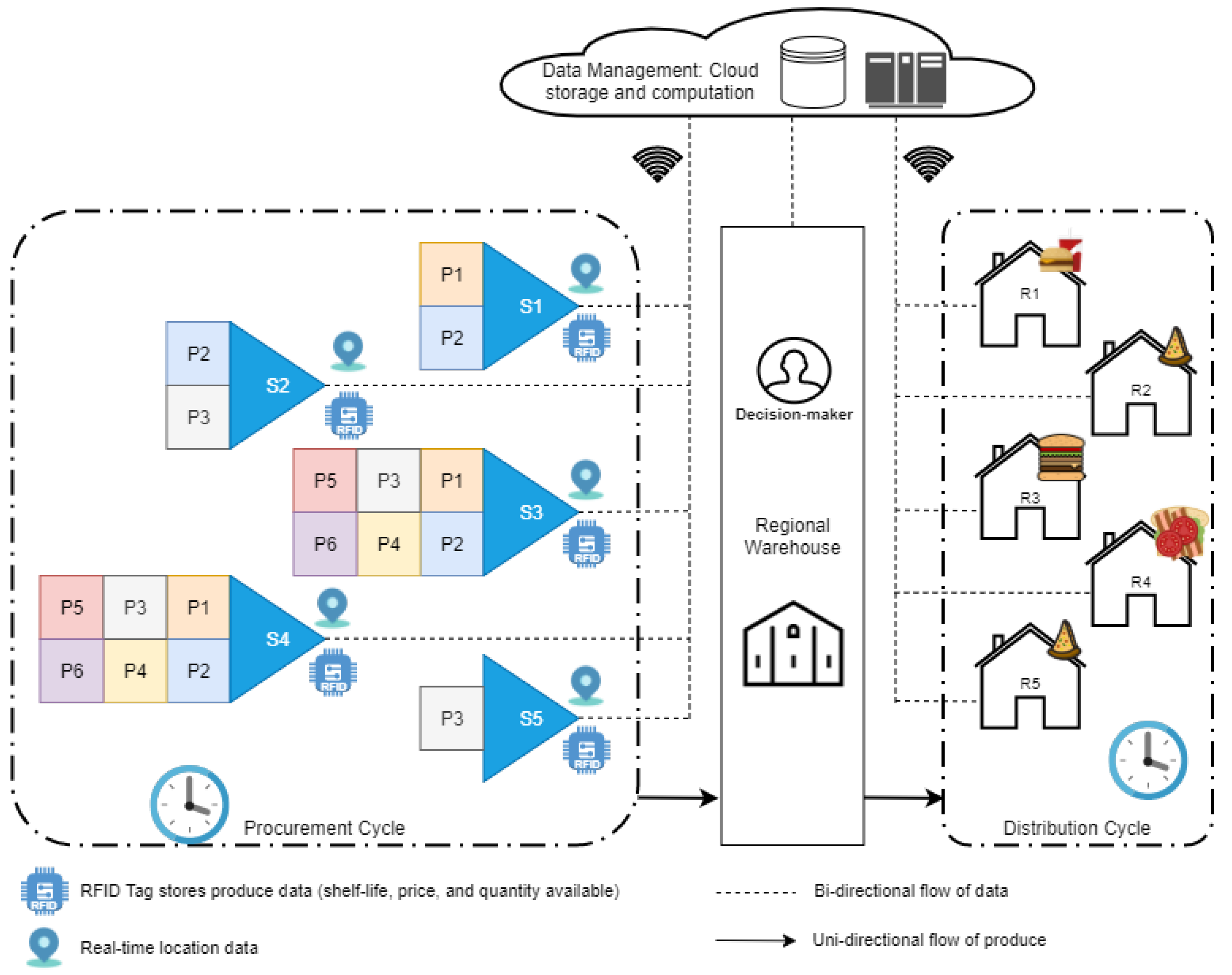


